
A New Model Averaging Approach in Predicting Credit Risk Default


1
Department of Economics and Management, University of Bergamo, 24129 Bergamo, Italy
2
Faculty of Economics and Social Sciences, Marche Polytechnic University, 60121 Ancona, Italy
*
Author to whom correspondence should be addressed.
Risks 2021, 9(6), 114; https://0-doi-org.brum.beds.ac.uk/10.3390/risks9060114
Submission received: 23 April 2021
/
Revised: 28 May 2021
/
Accepted: 1 June 2021
/
Published: 8 June 2021
Abstract
:The paper introduces a novel approach to ensemble modeling as a weighted model average technique. The proposed idea is prudent, simple to understand, and easy to implement compared to the Bayesian and frequentist approach. The paper provides both theoretical and empirical contributions for assessing credit risk (probability of default) effectively in a new way by creating an ensemble model as a weighted linear combination of machine learning models. The idea can be generalized to any classification problems in other domains where ensemble-type modeling is a subject of interest and is not limited to an unbalanced dataset or credit risk assessment. The results suggest a better forecasting performance compared to the single best well-known machine learning of parametric, non-parametric, and other ensemble models. The scope of our approach can be extended to any further improvement in estimating weights differently that may be beneficial to enhance the performance of the model average as a future research direction.

1. Introduction
The field of credit risk has grown significantly over the last few decades both in terms of scholarly articles and the availability of tools to measure and manage credit risk management (Altman and Saunders 1998).
The current trends in credit risk management advocate the use of classification techniques Baesens et al. (2003), Brown and Mues (2012) for credit default prediction that are parametric, non-parametric, and ensemble models, given their suitability to analyze large sample size data and provide better ways to capture complex relationship from the data (Figini et al. 2017; Lessmann et al. 2015; Butaru et al. 2016; Alaka et al. 2017).
However, the standard approach Fragoso et al. (2018) in making predictions does not identify a single best model for addressing classification, a limitation in data for several plausible combinations of predictors Breiman (1996), and the availability of different modeling approaches makes it difficult to select only one best model (e.g., Hastie et al. 2009; Kuhn and Jhonson 2013; Chipman et al. 2010).
One way to address such a limitation is to use the model averaging technique Graefe et al. (2014), Bates and Granger (1969), an approach that provides high discriminatory power and a high precision compared to other traditional statistical methods Granger and Ramanathan (1984), Hansen (2007), Nelder and Wedderburn (1972).
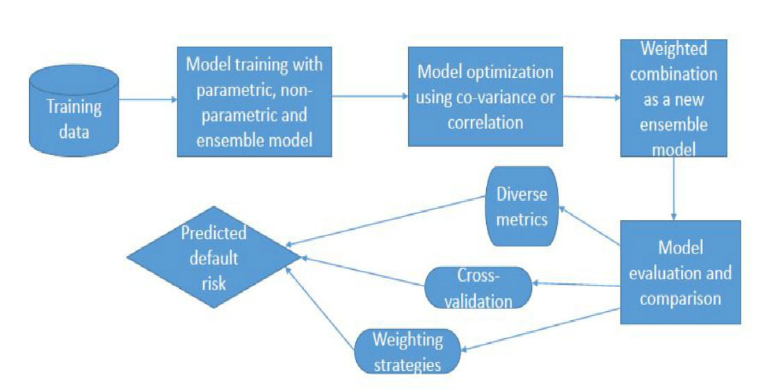
Although model averaging is an efficient approach to tackle the above different limitations, the empirical implementation of model-averaging methods is difficult considering model parametrization. This paper aims at addressing this issue by proposing an approach to implement a model average technique that linearly combines a set of weighted models based on a prediction of averaging correlative/co-variate models. Compared to existing approaches, the proposed model does not focus on parametrization to avoid possible criticism as summarized in Banner and Higgs (2017).
To implement the technique, we rely on a novel methodology based on the solution of a quadratic programming problem. The proposed approach exploits the idea that the best average model is the one that minimizes the co-variance between the errors of the single models (parametric models, non-parametric models, and ensemble model average).
The robustness of the proposed model is compared against a diverse set of key performance measures such as hmeasure (H), area under the receiver operating characteristic curve (AUC), area under the convex hull (AUCH), minimum error rate (MER), and minimum cost weighted error rate (MWL) (see, e.g., Hand 2009 for details on such metrics). This helps to examine predictive capability, discriminatory power, and stability of the results. The results obtained from the proposed model demonstrate better performance compared to well-known models.
In principle, the results obtained from the proposed idea on the dataset of a financial institution can be generalized to other groups of entities for credit risk assessment (probability of default) since almost all entities have similar nature of dataset with a class imbalance of default risk even if there is a difference in the set of explanatory variables for the different dataset.
The observation period of the sample used for the analysis in this paper is 24 months for two consecutive years from 2016 to 2018, and the sample studied reflects the economic and social behavior of those Italian customers who applied for loans.
It is very likely to have a similar level of performance on a dataset of other entities for credit risk assessment, specifically default risk parameters, since the proposed idea is not limited to a particular kind of dataset; in fact, the idea has high a possibility to solve classification problems in other domains.
The remainder of this paper is organized as follows. Section 2 presents the literature review relevant to the proposed research problem. Section 3 explains the proposal in detail as a piece of background information followed by a theoretical proposal in Section 4 and properties of the proposed model average in Section 4.2. Section 5 discusses the dataset and data handling method. Section 6 presents the results achieved from empirical findings followed by discussion in Section 7 and concluding remarks in Section 8. Appendix A provides additional useful information.
2. Literature Review
Most of the classification algorithms that can be broadly categorized as machine learning and artificial intelligence systems are often not used by the financial institution due to stronger requirements set up by regulatory Committee that supports the use of parametric models for a simple and clear interpretation of the results. Despite regulatory choice in suggesting the statistical framework Ewanchuk and Frei (2019), various literature supports the use of advanced models in assessing credit risk (Leo et al. 2019).
Alaka et al. (2017) addresses more sophisticated models for credit risk estimation and presents a systematic review of tool selection for analyzing bankruptcy prediction models.
Chakraborty and Joseph (2017) advocate the use of the machine learning model to detect financial distress using balance sheet information, and their study concludes a performance increase of 10 percentage points compared to the logistic regression model as a preferred classical approach of financial institutions.
Khandani et al. (2010) applied state-of-the-art of non-parametric machine learning models to predict the default of consumer credit risk by merging transactions and credit bureau data. Their work demonstrates that prediction of risk can be better improved using machine learning techniques in comparison to classical statistical approaches, and any subsequent loss of lenders therefore can significantly be improved.
Albanesi and Vamossy (2019) applied a deep learning approach as a combination of neural network and gradient boosting for high-dimensional data to predict the default of consumer risk. Their work shows superior performance compared to logistic regression models and is also able to adapt to the aggregate behavior of default risk easily.
Bacham and Zhao (2017) compared the performance of machine learning models with industry-developed algorithms such as Moody’s proprietary algorithm and suggested an improvement of 2–3 percentage points in the performance of the machine learning model. Their approach is a bit difficult to relate with the underlying firm characteristics in predicting default of credit risk, although credit-behavior-related variables increase the discriminatory power of the considered models.
Fantazzini and Figini (2009) proposed a non-parametric approach based on random survival forests in predicting credit risk default of small–medium enterprises. The performance comparison of their proposed model with the traditional logistic regression model reveals a weak relationship of the performance between training and testing samples, thereby suggesting an over-fitting problem, which is mainly due to contrasting testing sample performance of logistic regression better than their proposed random survival models.
Several other studies, such as Kruppa et al. (2013), Yuan (2015), Barboza et al. (2017), Ampountolas et al. (2021), and Addo et al. (2018), confirm superior performance for prediction of credit risk using machine learning compared to any other statistical approach.
The literature on the non-statistical model often suggests the dependence on the bias of contributing models as well as their weights for the difference between the expectation of the averaged predictions and truth. However, the underlying assumption for statistical model averaging literature does not have any bias, and their contribution is often less interesting (e.g., Burnham and Anderson 2002).
Reducing bias is often cited as the primary motivation in many of the literary works for model averaging, especially those related to process models (e.g., Solomon et al. 2007; Gibbons et al. 2008; and Dietze 2017). Due to the nature of predictions, weights are quadratic in terms rather than linear, as understanding deeply the right way of estimating weights Breiman (1997) brings a lot of benefits to the model averaging approach. To obtain a good estimator for the optimal weight in the first place is a further open problem apart from the error of the estimate, and there is no such closed solution available, including the case of linear models (Liang et al. 2011).
Broadly speaking, the literature supports parametric, non-parametric, and ensemble model-averaging approaches. The idea of model averaging appears of interest to reduce prediction error as well as to better reflect model selection (Buckland et al. (1997); Madigan and Raftery (1994)) uncertainty. Claeskens et al. (2016) assumed that estimated model weights are useful in general, being bias-free with similar prediction variance, but they do not necessarily imply that estimated equal weights are superior. To our knowledge, this area of research could be enlarged by proposing several ideas to select weights, and the methodological approach described in this paper is an effort towards this direction to improve model predictive performance.
3. Background Proposal
In recent years, several multi-model methods have been proposed to account for uncertainties arising from input parameters and the definition of model structure. In this paper, we propose a novel methodology for a model average based on the solution of a quadratic programming problem. Let us suppose as k different models for the dependent variable y.
For each model under consideration, the estimated error can be evaluated as , where is the estimated value of y for any model k. Based on , it is possible to estimate the co-variance or correlation matrix to set up an optimization problem that seeks to minimize the error between models.
The optimization problem can be solved for both co-variance and correlation matrix. We need to understand if one of the two provides better results and preferring co-variance matrix enhances proposed model performance slightly better with compare to correlation matrix as evident in their empirical results in Section 6. In general, the optimization problem is indifferent if defined for a non-singular positive definite square matrix of the models. One way to solve the optimization problem could be to find the vector of weights that minimizes the co-variance between the alternative models.
An average of models can improve the performances of single models when the errors of the single models are negatively correlated. Roughly speaking, an average model improves performance compare to single models when an error of the single model is counterbalanced by a good prediction of some other model. Following this idea, the best average model is the one that minimizes the co-variance between the errors of the single models.
4. Theoretical Proposal
4.1. Notation and Assumptions
is the co-variance matrix of the errors with . is a positive, definite, symmetric and, as a consequence, non-singular matrix. w is the column vector of the weights. The average model is defined as where is the kth entry of vector w, is the column vector of ones and superscript T represents transpose of a matrix. In accordance with our considered model average technique, we formulate the following optimization problem
Solving analytically the optimization problem produces an optimal vector of weights
where
For the optimization problem stated above, the first-order conditions are necessary and sufficient for the optimality of , which is obvious due to the assumptions made on co-variance matrix .
The analytical solution assumes no bias and therefore ignores the problem that weights are random variate since weights sum to one in constraint. Doing this does not necessarily ensure weights to be positive, nor we want to use some rarely used method that adjusts for correlation in predictions (e.g., assigning lower weights to highly correlated models, dividing weights if any identical model prediction is added to the set, and henceforth reducing weights due to additional inclusion of the model).
No single model guarantees achieving consistently lower error rates since many of the model averaging techniques stated in the literature are not easy to implement, and potentially one of the reasons for extensive use of ensemble techniques like bagging and boosting (Breiman (2001b); Friedman (1999)).
Keeping this point in mind, our effort in proposing the idea of model averaging is unique and simple in the sense that it is easy to implement and offers the possibility to combine or average out models of different natures in the model space (be it parametric, non-parametric and or models) rather intuitively.
A few of the main advantages of the proposed idea are (i) improvements in the performances compared to single original models (already tested within the empirical framework), (ii) the closed form for the solution of the optimization problem, and (iii) a simple interpretation of the whole theoretical structure.
A few of the limitations of the proposed idea are as follows. (i) First is interpretation of the negative weights. When the weight associated with a model is negative, intuitively we are doing the opposite compared to what the model suggests doing. It is clear that negative weights are useful to artificially create negative co-variances between models, providing the possibility to achieve lower values of co-variance. (ii) Second is that if for are bounded (for example in the case of the probability of default when modeling credit risk), the proposed approach does not guarantee that respects the bounds.
In order to overcome the potential shortcomings described above, we can frame new optimization problem as follows,
This helps to overcome both the shortcomings on the interpretation of the negative weights and the bounded value for .
In this case, it is trivial to prove that is bounded between the minimum and the maximum values of the single models because the average model is a convex linear combination of the original models. Two of the possible limitations of the new optimization problem with different constraints include the availability of no closed-form solution for the problem and that a growing number of restrictions penalizes the performances of the average model.
Moreover, an increase in additional constraints like the following,
does not guarantee the estimation of positive weights, nor does it achieve minimum prediction error. Many extensions are possible, of which one standard extension could be to allow the weights to be negative, optimal, equal, random, or squared for diverse options and compare the performance of weighted model based on each of these different weighting strategies.
Assuming such a weighting strategy as a possible extension, we evaluated the performance of the weighted model using different weighting strategies, and the results at hand favor the proposed analytical weights based on Equation (1) as a better choice compared to all other weighting strategies.
4.2. Properties: The Proposed Model Average
So far, our discussion was focused on co-variance and other methods that play a crucial role in the estimation of weights and construction of model average. In this sub-section, the focus of our discussion is how weighted models behave or vary when there is correlation or no correlation between models.
Let us assume first the case of uncorrelated models in the model-averaging system where we refer to the properties of variance and assume models are independent. One of the possible ways to obtain optimal weight in the weighted model system if the models are not correlated is to construct the model as a linear combination of the individual model.
Therefore, we consider a model average as a linear combination of its members as and are normalized to 1 to generate the following relationship:
Using the above equation, we can find the optimal coefficient as weights to the model by minimizing error and can be converted into an optimization problem, as evident in the following equation:
This could lead to a lesser extent of underestimation of the statistical properties of the model average if the optimal weight from the coefficient is not considered.
Therefore, we can ask ourselves if there is any way that ensures that the variance of the weighted model is lower than an individual model’s variance. To understand more of this, take a case of two models with variance such that their combined variance is less than a single model’s variance.
The combination process works best if the variance between models is not too large; otherwise, it is not possible to achieve weighted model variance lower than individual models. In this respect, we propose the following theorem and its proof.
Theorem: If the combined variance of two models is less than a single model’s variance, then the combination process works best only when the variance between models is minimized; otherwise, it is not possible to achieve average model variance lower than individual models. This is true if the models among themselves are not correlated, as it is possible to obtain the variance of average model lower than single models, as evident in the following inequality, where v() simply denotes the variance of the model.
Proof.
Let us say that . Therefore, we can further say that
which in turn proves that . □
The idea mentioned in the above theorem can be generalized to models that are correlated among each other and for which it is possible to obtain general bounds for optimal variance using the following equation,
The proof sketched in the theorem above for uncorrelated models can equally be explored for correlated models by showing equivalent estimation for optimal variance according to the following,
5. Data Description
The dataset used for this study come from one of the leading financial institutions where the dependent variable “ClientStatus” is represented by binary values that take “0 (good customer)” and “1 (bad customer)”. A priori probability for the target variable shows 96.11% of class label 0 and 3.9% of class label 1. The observation period of the dataset is 24 months for two consecutive years from 2016 to 2018, and the sample studied reflects the economic and social behavior of those Italian customers who applied for loans.
The data are composed of 40,000 observations and 30 explanatory variables. The explanatory variable is mainly categorized as information about socio-demographic characteristics, customer equipment, customer history, and other things related to customer behavior. See Appendix A for more details on explanatory variables.
The prior distribution of the class in the dependent variable is imbalanced and needs treatment before being put to the predictive modeling task Kuhn and Jhonson (2013). Re-sampling the training set (under-sampling or over-sampling), using k-fold cross-validation in the right way, ensembling different resampled datasets, resampling with different ratios, clustering the majority class, or designing any different model, offers a few of the popular alternatives to deal with the data imbalance problem Batista et al. (2004).
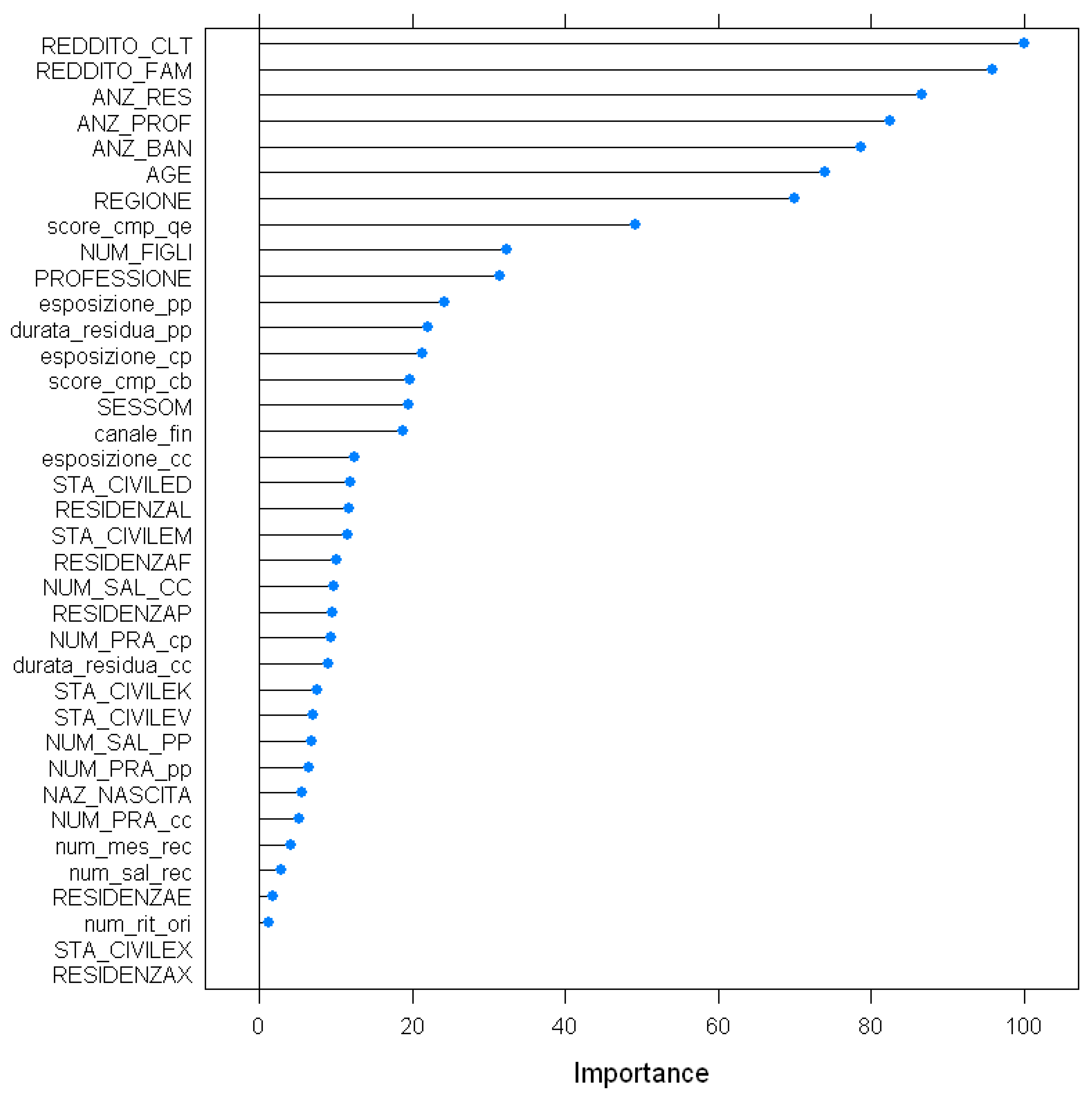
There are several ways to do feature selection or feature engineering, and in this respect, we choose to sketch variable importance plots using built-in functions of boosted classification trees. The features are ranked on an importance scale of 1 to 100. We restricted them to include only the top 10 ranked features in the model for getting better performance after evaluating different possibilities of feature inclusion. The features ranked are reported in Appendix A.
In this context, we chose to treat the imbalance problem of the class distribution using one of the latest preferred techniques called SMOTE (synthetic minority over-sampling technique). SMOTE (Chawla et al. 2002) creates synthetic observations based on existing minority observations that work on the principle of k-nearest neighbors Henley and Hand (1997). It generates new instances that are not just copies of the existing minority class; in fact, the rule is to take samples of feature space for each target class and its nearest neighbors. In this way, it increases the features available to each class and makes the samples more general and balanced.
A few of the alternatives other than the over-sampling and under-sampling technique for class imbalance problem is to use the Grabit model (gradient tree boosting to the Tobit model), which creates an auxiliary sample to enhance predictive accuracy (see, for details, Sigrist and Hirnschall 2019).
6. Results
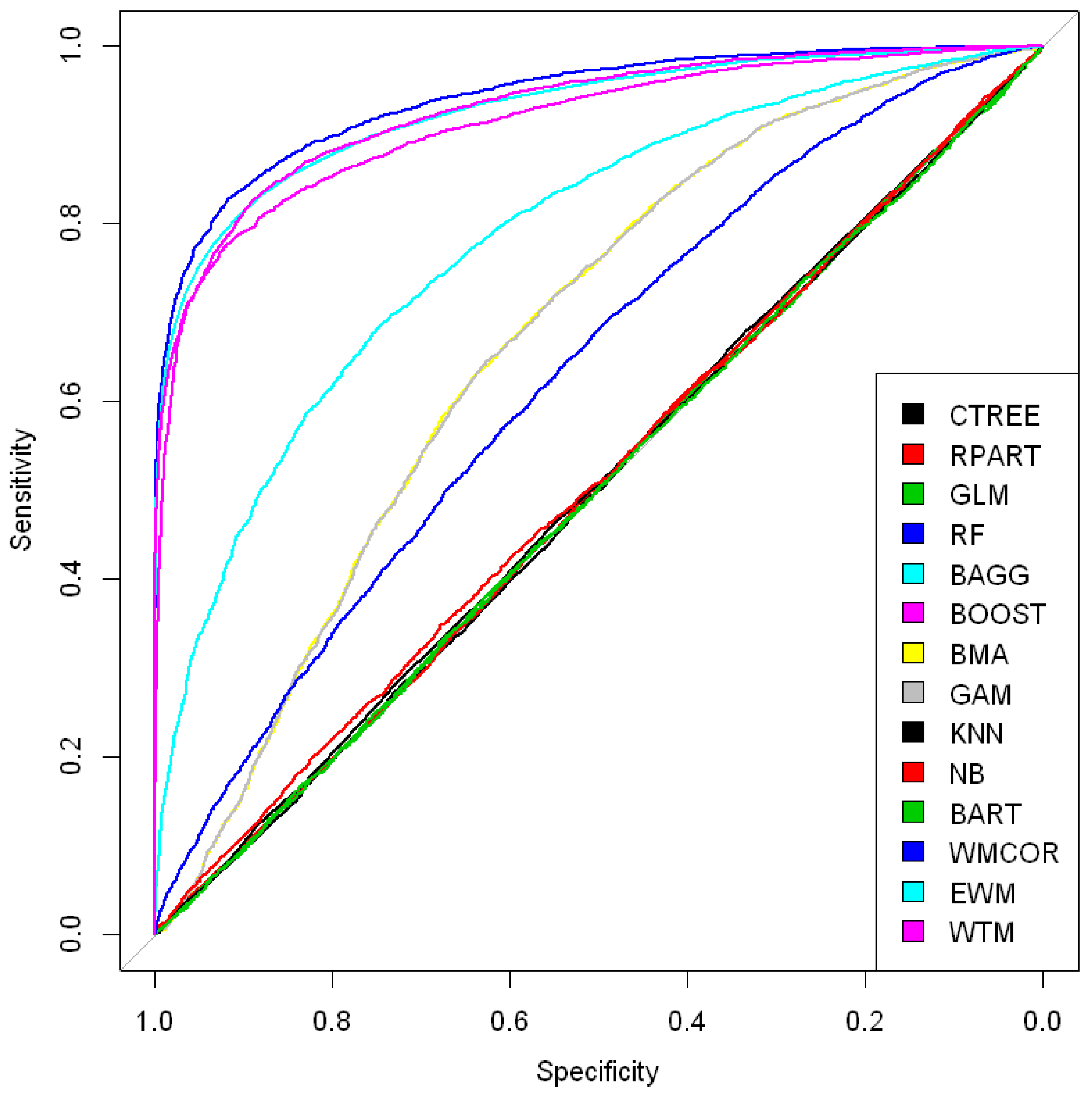
The considered list of models were implemented using a k-foldapproach (k = 10), and comprise a diverse set of models like conditional inference trees (CTREE), recursive partitioning and regression trees (RPART), generalized linear model (GLM), random forest (RF), bootstrap aggregating (BAGG), boosting (BOOST), Bayesian moving average (BMA), generalized additive model (GAM), k-nearest neighbors (KNN), naive Baye’s (NB), Bayesian additive regression trees (BART), and proposed weighted model based on co-variance (WTM). Figure 1 and Figure 2 report the performance comparison as an ROC curve that suggests the proposed model WTM as a better model in enhancing predictive performance compare to other well-known model and weighting techniques.
Figure 1 shows the ROC (receiver operating characteristic) curve comparison of different models (parametric, non-parametric, ensemble model, and average model), and it is some performance difference and overlapping are obvious. The model choice becomes an uncertain and daunting task in such a situation. To avoid such uncertainties to a greater extent, our proposed model provides an alternative that is easy to implement and robust in enhancing the performance of the combined model for predicting credit risk default.
Several performance metrics reflecting the accuracy and error of the model were assessed on out of sample data as reported in Table 1 and Table 2. Table 3 does a robustness check of the analytical weights in the proposed model (WTM) with different possibilities of weighting strategies. H (hmeasure), AUC (area under curve), AUCH (area under convex hull), Sens.Spec95 (sensitivity at 95 percent specificity), and Spec.Sens95 (Specificity at 95 percent sensititvity) are related metrics. MER (minimum error rate) MWL (minimum weighted loss) are error-related metrics.
Table 1 records the performance of the individual model and the proposed model WTM. H (hmeasure), AUC (area under the curve), AUCH (area under convex hull), Sens.Spec95 (sensitivity at 95 percent specificity), and Spec.Sens95 (Specificity at 95 percent sensitivity) are accuracy-related metrics. The higher the value of the metrics is, the better the performance of the model is, and such numbers are kept in bold text. From Table 1, looking at the H measure, RandomForest (RF), and the proposed weighted model based on the co-variance approach (WTM) shows better performance compared to other models. In terms of AUC value, RandomForest (RF) has slightly better performance that is very close to the values of Bagging (BAGG), Boosting (BOOST), and therefore is highly comparable. The same is true with AUCH values.
Table 2 records prediction-error-related performance measures of the individual model and the proposed one. MER (minimum error rate) and MWL (minimum weighted loss) are error-related metrics of the model. The lower the value is, the better the performing model is. From Table 2, one can see that the best-performing models are RandomForest (RF), Bagging (BAGG), Boosting (BOOST), and the proposed weighted model (WTM).
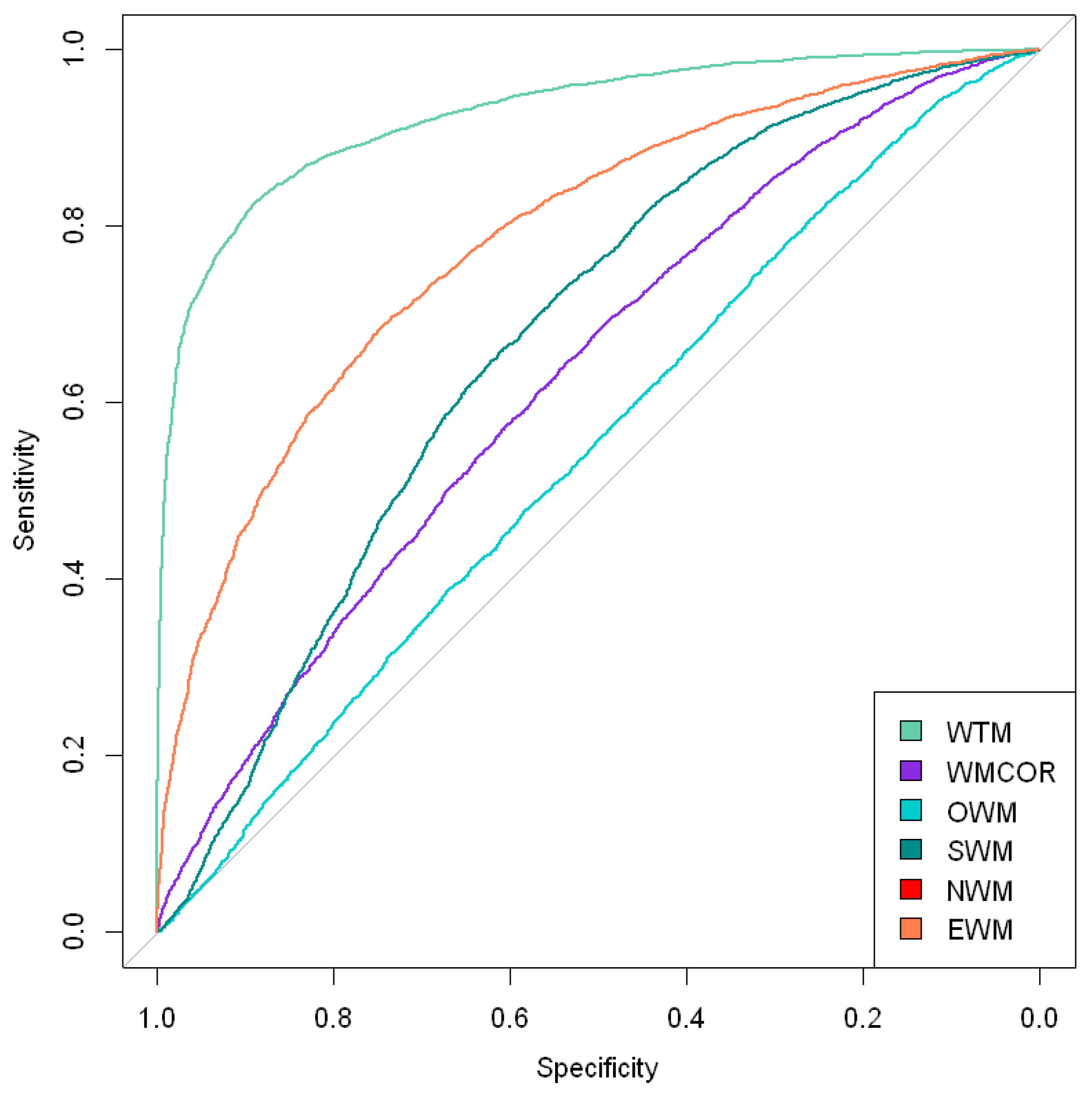
Table 3 lists the proposed model (WTM) comparison against all other weighting techniques that could have been useful for a robustness check like weighting approach using correlation (WMCOR), optimal weight (OWM), squared weight (SWM), negative weight (NWM), and equal weight (EWM). Their performance comparison is also reported in Figure 2. The performance comparison in Figure 2 and Table 3 suggests the proposed approach (WTM) as providing better-chosen weights for developing a better ensemble model average compared to other weighting techniques.
Table 4 and Table 5 illustrate an example of a confusion matrix to compare the proposed model (WTM) with one of the well-known models, random forest (RF) Breiman (2001a). The comparison is done with k-fold cross-validation in this context, which assigns a random sample to different folds, and any difference in the class instances for observed and predicted values for the model under comparison is due to sample size difference of cross-validation. The benefits of cross-validation works differently than the usual splitting of train and test set, since it helps to generalize the performance to an independent set by overcoming any selection bias and overfitting problem.
The comparison in the table suggests that the proposed model (WTM) is better at classifying class instances compared to well-known models such as the random forest. One could argue here as to why we are not averaging the confusion matrix for all folds. The reason for not doing it is to simply avoid bias that arises due to the difference in a sample size of all folds, and summing up the confusion matrix does not provide any additional information regarding the robustness of the classifier.
A broader picture of decision making based on some classifier performance should be done using several diverse metrics such as the one reported in Table 1 and Table 2, as this helps to see how different models’ performances overlap or diverge among each other, which is needed for a robustness check of the proposed classifier.
In a situation where the performances of classifiers overlap or intersect with each other, it is difficult to point out the best model, although to a smaller extent, RandomForest and classification trees might give a smaller prediction error than the proposed model (WTM), but their performance inconsistencies is often well-known. However, it is interesting to point out that the proposed model (WTM), overall, in terms of reflecting different accuracy and error performance metrics, outperforms all other well-known models.
To make the proposed approach (WTM) more competitive in comparison to well-known models, a different approach is needed to estimate weights differently from the proposed optimization problem that might bring additional enhancement in the performance of the WTM model.
7. Discussion
The model averaging approach is primarily useful in reducing prediction errors but may not necessarily do so in every context. The reason for this is that a few individual models among the pool of models do not contribute to the decrease in co-variance and average bias. This can be offset using a proper or diverse technique for estimating weights that in turn helps in adjusting the additional variance from weaker models.
The literature is full of different information criteria that advocate the right way of estimating weights. In our opinion, however, none of the information criteria are ideal to apply to every single problem. Therefore, a continuous discussion on evolving the theories and techniques of information criteria will be an important step in this direction.
The traditional approach suggests using the single best model and therefore ignores model uncertainty that may arise due to model structure and assumptions. Therefore, relying on the single best model with confidence is not a good idea as it may have adverse consequences. The committee of diverse models offers enhanced performance if it is based on model average techniques (see, for instance, Figini et al. 2016; Figini and Giudici (2017)).
Model averaging studies are dominated by two approaches, which are the Bayesian and the frequentist approaches. Any different approach, such as the one proposed in this paper, is an attempt to offer a technique that is effective to solve the diverse problems of classification. Our proposed model-averaging technique can be considered as a cutting tool that does not take parameter values for averaging.
In this sense, we make the approach flexible to work on many different problems. There is contradicting opinion if the model averaging technique is any ensemble technique, unlike boosting and bagging. Such a belief is mostly because model averaging is not straightforward from the computational point of view and lacks generalization abilities that can solve different problems.
However, our work in this paper strongly supports the argument that the model averaging technique outperforms bagging and boosting in many situations, especially if there is model uncertainty, model bias, and high variance and if the dataset is imbalanced. To further emphasize our proposed idea, we can say that it is similar to the ensemble technique and offers various possibilities to enhance the performance of any machine learning model.
The main idea of any ensemble technique is to weigh individual classifiers and combine them in a way to produce output that is better than individual classifiers at predicting the task. Our proposed ensemble technique is characterized by diverse classifiers, which makes any ensemble technique efficient to enhance predictive performance.
The diversity of classifiers offers a serious advantage in developing an effective model averaging or ensemble technique, but its inter-relationship with predictive output and errors will be an important point of investigation from a future perspective.
Making an effort to keep understanding of the ensemble model simple to non-technical people would be also a wise step in this direction. Moreover, until today, model averaging studies have favored non-parametric methods for correctly estimating predictive errors, and there is a lack of reliable analytical methods in this respect to compute frequentist confidence intervals(p-values) on averaged model predictions.
Parametric methods based on AIC (Akaike information criterion) and BIC (Bayesian information criterion) may give better performance. However, this is not always true as non-parametric methods have an advantage under general considerations. Parametric methods improve predictive error if any fixed or estimated weights are used.
A major part of applied machine learning is to understand the tips and tricks around model selection. Given a large choice of models for selection, how one model statistically differs from other models is a question of continuous investigation and testing.
The field of machine learning is evolving rapidly with its inter-connection to optimization theories and multi-objective optimization. Optimization plays a crucial role in minimizing or maximizing the different objective functions of interest that influence the performance of the learning algorithm.
8. Concluding Remarks
In this study, we have compared parametric, non-parametric, and ensemble models with our proposed idea, and the experiment on real data suggests that the proposed model is able to enhance performance as compared to a few of the well-known models when different modeling cultures are adopted (see, for example, Breiman 2001b).
A new weighted ensemble model approach introduced in this paper and the methodological development could be of interest for different practical implications in other domains. For instance, the proposed idea advocates a new direction of model average to improve predictive performance without necessarily taking any parameter estimation into account and is a rather simple, prudent, and intuitive method of model combination for any given set of diverse models one wishes to work with.
The proposed approach has an advantage over both well-known parametric and non-parametric models. The only limitation of this idea could be explored in estimating weights differently, which may further enhance the performance of the proposed model, and any effort in this direction would bring an additional advantage.
Moreover, at present, non-parametric methods such as cross-validation remain reliable for estimation of predictive errors, and there is a lack of reliable analytical methods to compute frequentist confidence intervals (p-values) on averaged model predictions. Parametric methods based on AIC and BIC may give better performance, but this is not always true, as non-parametric methods have an advantage under general considerations to improve predictive error if any fixed or estimated weights are used.
A single model may serve the purpose supported with a good underlying economic theory but is prone to the model uncertainty problem, and to answer such uncertainties, ensemble model average techniques such as the one proposed in this paper serve as effective tools for various predictive tasks and are not limited only to credit risk assessment.
The model averaging technique may decrease prediction error to a greater extent, but the primary benefits of doing so lie in decreasing co-variance and mean bias of contributing models. Any further improvement in the estimation of weights does reduce the weight of weaker models but could reduce the benefits of model averaging at the cost of additional variance, which may be a point of interesting discussion as a future research direction.
Author Contributions
Conceptualization, P.N.J.; Formal analysis, P.N.J. and M.C.; Funding acquisition, M.C.; Methodology, P.N.J.; Software, P.N.J.; Supervision, M.C.; Writing—original draft, P.N.J.; Writing—review & editing, M.C. Both authors have read and agreed to the published version of the manuscript.
Funding
Marco Cucculelli acknowledges the financial support from Università Politecnica Delle Marche, Ancona, Italy.
Data Availability Statement
Not applicable.
Conflicts of Interest
The authors declare no conflict of interest.
Appendix A

Table A1.
Socio-economic variable description.
| Variable | Description | Type |
|---|---|---|
| AGE | Loan applicant age | discrete |
| REGIONE | Location details | categorical |
| ANZ_BAN | Age of the current account (expressed in years) | discrete |
| RESIDENZA | Type of Residence (owner or tenant) | categorical |
| ANZ_RES | Seniority of residence in the current residence (expressed in years) | discrete |
| STA_CIVILE | Marital status (married, single, divorced …) | categorical |
| NUM_FIGLI | Number of child | discrete |
| SESSO | Gender | categorical |
| REDDITO_CLT | Applicant income | continuous |
| REDDITO_FAM | Family income | continuous |
| PROFESSIONE | Profession | categorical |
| NAZ_NASCITA | Country of birth | categorical |
| ANZ_PROF | Working seniority (expressed in years) | discrete |
Table A2.
Client equipment variable description.
| Variable | Description | Type |
|---|---|---|
| CANALE_FIN | Financing channel (agency, web, telephone …) | categorical |
| NUM_PRA_PP | Current Personal Loans—number of practices | discrete |
| esposizione_pp | Current personal loans—residual amount on the balance | continuous |
| durata_residua_pp | Current personal loans—residual duration to balance | continuous |
| NUM_PRA_CC | Total finalized loans in progress—number of practices | discrete |
| esposizione_CC | Total finalized loans in progress—remaining balance | continuous |
| durata_residua_CC | Total finalized loans in progress—residual maturity at the balance | continuous |
| NUM_PRA_CP | Card—Customer holding card | discrete |
| esposizione_CP | Card—Credit Card Display | continuous |
Table A3.
Client history variable description.
| Variable | Description | Type |
|---|---|---|
| NUM_SAL_PP | Personal loans paid in the last 24 months—number of files | discrete |
| NUM_SAL_CC | Finalized loans paid in the last 24 months—number of practices | discrete |
Table A4.
Client behavior variable description.
| Variable | Description | Type |
|---|---|---|
| num_men_rit | number of late payments from origin (in months) | discrete |
| score_cmp_qe | internal behavioral score | continuous |
| score_cmp_cb | credit bureau behavioral score | categorical |
| num_sal_rec | number of recovery ascents in the last 12 months | discrete |
| num_mes_rec | number of months to recovery in the last 12 months | discrete |
Figure A1.
Feature importance graphical presentation.

References
- Addo, Peter Martey, Dominique Guegan, and Bertrand Hassani. 2018. Credit Risk Analysis Using Machine and Deep Learning Models. Risks 6: 38. [Google Scholar] [CrossRef] [Green Version]
- Alaka, Hafiz A., O. Lukumon Oyedele, Hakeem A. Owolabi, Vikas Kumar, Saheed O. Ajayi, Olugbenga O. Akinade, and Muhammad Bilal. 2017. Systematic review of bankruptcy prediction models: Towards a framework for tool selection. Expert Systems with Applications 94: 164–84. [Google Scholar] [CrossRef]
- Albanesi, Stefania, and Domonkos Vamossy. 2019. Predicting Consumer Default: A Deep Learning Approach. CEPR Discussion Papers 13914, C.E.P.R. Discussion Papers. London: CEPR. [Google Scholar]
- Altman, Edward I., and Anthony Saunders. 1998. Credit risk measurement: Developments over the last 20 years. Journal of Banking and Finance 21: 1721–42. [Google Scholar] [CrossRef] [Green Version]
- Ampountolas, Apostolos, Titus Nyarko Nde, Paresh Date, and Corina Constantinescu. 2021. A Machine Learning Approach for Micro-Credit Scoring. Risks 9: 50. [Google Scholar]
- Bacham, Dinesh, and Janet Zhao. 2017. Machine Learning: Challenges, Lessons, and Opportunities in Credit Risk Modeling. Moody’s Analytics Report. Moody’s Analytics risk perspectives, Managing disruption. Volume 9, Available online: https://www.moodysanalytics.com/risk-perspectives-magazine/managing-disruption/spotlight/machine-learning-challenges-lessons-and-opportunities-in-credit-risk-modeling (accessed on 3 June 2021).
- Baesens, B., T. Van Gestel, S. Viaene, M. Stepanova, J. Suykens, and J. Vanthienen. 2003. Benchmarking state-of-the-art Classification algorithms for credit scoring. Journal of the Operational Research Society 54: 627–35. [Google Scholar] [CrossRef]
- Banner, Katharine M., and Megan D. Higgs. 2017. Considerations for assessing model averaging of regression coefficients. Ecological Applications 27: 78–93. [Google Scholar] [CrossRef] [PubMed] [Green Version]
- Barboza, Flavio, Herbert Kimura, and Edward Altman. 2017. Machine learning models and bankruptcy prediction. Expert Systems with Applications: An International Journal 83: 405–17. [Google Scholar] [CrossRef]
- Bates, John M., and Clive W. J. Granger. 1969. The combination of forecasts. Journal of the Operational Research Society 20: 451–68. [Google Scholar] [CrossRef]
- Batista, Gustavo EAPA, Ronaldo C. Prati, and Maria Carolina Monard. 2004. A study of the behavior of several methods for balancing machine learning training data. ACM SIGKDD Expolorations Newsletter 6: 20–29. [Google Scholar] [CrossRef]
- Breiman, Leo. 1996. Bagging predictors. Machine Learning 24: 123–40. [Google Scholar] [CrossRef] [Green Version]
- Breiman, Leo. 1997. Arcing The Edge. Technical Report 486. Berkeley: Statistics Department, University of California. [Google Scholar]
- Breiman, Leo. 2001a. Random Forests. Machine Learning 45: 5–32. [Google Scholar] [CrossRef] [Green Version]
- Breiman, Leo. 2001b. Statistical Modeling: The Two Cultures (with comments and a rejoinder by the author). Statistical Science 16: 199–231. [Google Scholar] [CrossRef]
- Brown, Iain, and Christophe Mues. 2012. An experimental comparison of classification algorithms for imbalanced credit scoring data sets. Expert Systems with Applications: An International Journal 39: 3446–53. [Google Scholar] [CrossRef] [Green Version]
- Buckland, Steven T., Kenneth P. Burnham, and Nicole H. Augustin. 1997. Model selection: An integral part of inference. Biometrics 53: 603–18. [Google Scholar] [CrossRef]
- Burnham, Kenneth P., and David R. Anderson. 2002. Model Selection and Multi-Model Inference: A Practical Information-Theoretical Approach, 2nd ed.Berlin and Heidelberg: Springer. [Google Scholar]
- Butaru, Florentin, Qingqing Chen, Brian Clark, Sanmay Das, Andrew W. Lo, and Akhtar Siddique. 2016. Risk and risk management in the credit card industry. Journal of Banking and Finance 72: 218–39. [Google Scholar] [CrossRef] [Green Version]
- Chakraborty, Chiranjit, and Andreas Joseph. 2017. Working Paper No. 674 Machine Learning at Central Banks. Bank of England working papers. London: Bank of England. [Google Scholar]
- Chawla, Nitesh V., Kevin W. Bowyer, Lawrence O. Hall, and W. Philip Kegelmeyer. 2002. SMOTE: Synthetic Minority Over-sampling Technique. Journal of Artificial Intelligence Research 16: 321–57. [Google Scholar] [CrossRef]
- Claeskens, Gerda, Jan R. Magnus, Andrey L. Vasnev, and Wendun Wang. 2016. The forecast combination puzzle: A simple theoretical explanation. International Journal of Forecasting 32: 754–62. [Google Scholar] [CrossRef] [Green Version]
- Dietze, Michael C. 2017. Ecological Forecasting. Princeton: Princeton University Press. [Google Scholar] [CrossRef]
- Ewanchuk, Logan, and Christoph Frei. 2019. Recent Regulation in Credit Risk Management: A Statistical Framework. Risks, MDPI, Open Access Journal 7: 40. [Google Scholar] [CrossRef] [Green Version]
- Sigrist, Fabio, and Hirnschall Christoph. 2019. Grabit: Gradient tree-boosted Tobit models for default prediction. Journal of Banking and Finance 102: 177–92. [Google Scholar]
- Fantazzini, Dean, and Silvia Figini. 2009. Random survival forests models for sme credit risk measurement. Methodology and Computing in Applied Probability 11: 29–45. [Google Scholar] [CrossRef]
- Figini, Silvia, and Paolo Giudici. 2017. Credit risk assessment with Bayesian model averaging. Communications in Statistics—Theory and Methods 46: 9507–17. [Google Scholar] [CrossRef]
- Figini, Silvia, Bonelli Federico, and Giovannini Emanuele. 2017. Solvency prediction for small and medium enterprises in banking. Decision Support Systems 102: 91–97. [Google Scholar] [CrossRef]
- Figini, Silvia, Savona Roberto, and Vezzoli Marika. 2016. Corporate Default Prediction Model Averaging: A Normative Linear Pooling Approach. Intelligent System in Accounting, Finance, and Management 23: 6–20. [Google Scholar] [CrossRef]
- Fragoso, Tiago M., Wesley Bertoli, and Francisco Louzada. 2018. Bayesian Model Averaging: A Systematic Review and Conceptual Classification. International Statistical Review 86: 1–28. [Google Scholar] [CrossRef] [Green Version]
- Friedman, Jerome H. 1999. Greedy Function Approximation: A Gradient Boosting Machine. The Annals of Statistics 29: 1189–232. [Google Scholar]
- Gibbons, J. M., G. M. Cox, A. T. A. Wood, J. Craigon, S. J. Ramsden, D. Tarsitano, and N. M. J. Crout. 2008. Applying Bayesian model averaging to mechanistic models: An example and comparison of methods. Enviromental Modelling & Software 23: 973–85. [Google Scholar]
- Graefe, Andreas, J. Scott Armstrong, Randall J. Jones Jr., and Alfred G. Cuzan. 2014. Combining forecasts: An application to elections. International Journal of Forecasting 30: 43–54. [Google Scholar] [CrossRef]
- Granger, Clive W. J., and Ramu Ramanathan. 1984. Improved methods of combining forecasts. Journal of Forecasting 3: 194–204. [Google Scholar] [CrossRef]
- Hand, David J. 2009. Measuring classifier performance: A coherent alternative to the area under the ROC curve. Machine Learning 77: 103–23. [Google Scholar] [CrossRef] [Green Version]
- Hansen, Bruce E. 2007. Least squares model averaging. Econometrica 75: 1175–89. [Google Scholar] [CrossRef] [Green Version]
- Hastie, Trevor, Tibshirani Robert, and Jerome H. Friedman. 2009. The Elements of Statistical Learning: Data Mining, Inference, and Prediction, 2nd ed. Berlin and Heidelberg: Springer. [Google Scholar]
- Henley, W. E., and D. J. Hand. 1997. Construction of a k-nearest neighbour credit scoring system. IMA Journal of Management Mathematics 8: 305–21. [Google Scholar] [CrossRef]
- Hugh, A. Chipman, Edward I. George, and Robert E. McCulloch. 2010. BART: Bayesian additive regression trees. The Annals of Applied Statistics 4: 266–298. [Google Scholar]
- Khandani, Amir E., Adlar J. Kim, and Andrew W. Lo. 2010. Consumer credit-risk models via machine-learning algorithms. Journal of Banking and Finance 34: 2767–87. [Google Scholar] [CrossRef] [Green Version]
- Kruppa, Jochen, Alexandra Schwarz, Gerhard Arminger, and Andreas Ziegler. 2013. Consumer credit risk: Individual probability estimates using machine learning. Expert Systems with Applications 40: 5125–31. [Google Scholar] [CrossRef]
- Kuhn, Max, and Kjell Jhonson. 2013. Applied Predictive Modeling. Berlin and Heidelberg: Springer. [Google Scholar] [CrossRef]
- Lessmann, Stefan, Bart Baesens, Hsin-Vonn Seow, and Lyn C. Thomas. 2015. Benchmarking state-of-the-art classification algorithms for credit scoring: An update of research. European Journal of Operational Research 247: 124–36. [Google Scholar] [CrossRef] [Green Version]
- Liang, Hua, Guohua Zou, Alan T. K. Wan, and Xinyu Zhang. 2011. Optimal weight choice for frequentist model average estimators. Journal of the American Statistical Association 106: 1053–66. [Google Scholar] [CrossRef]
- Madigan, David, and Adrian E. Raftery. 1994. Model selection and accounting for model uncertainty in graphical models using Occam’s window. Journal of the American Statistical Association 89: 1535–46. [Google Scholar] [CrossRef]
- Leo, Martin, Suneel Sharma, and K. Maddulety. 2019. Machine Learning in Banking Risk Management: A Literature Review. Risks 7: 29. [Google Scholar]
- Nelder, John Ashworth, and Robert W. M. Wedderburn. 1972. Generalized Linear Models. Journal of the Royal Statistical Society 135: 370–84. [Google Scholar] [CrossRef]
- Solomon, S., D. Qin, M. Manning, M. Marquis, K. Averyt, M. M. B. Tignor, H. Leroy Miler Jr., and Z. Chen, eds. Climate Change 2007: The Physical Science Basis. Cambridge: Cambridge University Press.
- Yuan, Danny. 2015. Applications of Machine Learning: Consumer Credit Risk Analysis. Cambridge: DSpace, MIT. [Google Scholar]
Figure 1.
ROC curve of parametric, non-parametric, ensemble, and proposed weighted model.

Figure 2.
Proposed model using different weighting strategy.

Table 1.
Performance metrics reflecting the accuracy of the model.
| Metrics | CTREE | RPART | GLM | RF | BAGG | BOOST | BMA | GAM | KNN | NB | BART | WTM |
|---|---|---|---|---|---|---|---|---|---|---|---|---|
| H | 0.62 | 0.59 | 0.67 | 0.64 | 0.61 | 0.57 | 0.78 | 0.78 | 0.39 | 0.38 | 0.50 | 0.60 |
| AUC | 0.94 | 0.80 | 0.67 | 0.94 | 0.92 | 0.91 | 0.67 | 0.67 | 0.79 | 0.77 | 0.82 | 0.92 |
| AUCH | 0.94 | 0.80 | 0.67 | 0.94 | 0.92 | 0.91 | 0.67 | 0.67 | 0.79 | 0.77 | 0.82 | 0.92 |
| Sens.Spec95 | 0.24 | 0.15 | 0.04 | 0.63 | 0.50 | 0.48 | 0.20 | 0.20 | 0.03 | 0.05 | 0.04 | 0.58 |
| Spec.Sens95 | 0.10 | 0.07 | 0.05 | 0.78 | 0.77 | 0.73 | 0.06 | 0.06 | 0.03 | 0.06 | 0.04 | 0.73 |
Table 2.
Performance metrics reflecting error in the model.
| Metics | CTREE | RPART | GLM | RF | BAGG | BOOST | BMA | GAM | KNN | NB | BART | WTM |
|---|---|---|---|---|---|---|---|---|---|---|---|---|
| MER | 0.16 | 0.16 | 0.26 | 0.13 | 0.14 | 0.15 | 0.15 | 0.25 | 0.16 | 0.26 | 0.16 | 0.14 |
| MWL | 0.18 | 0.19 | 0.29 | 0.12 | 0.14 | 0.15 | 0.16 | 0.26 | 0.19 | 0.28 | 0.19 | 0.14 |
Table 3.
Proposed model comparison against all other weighting techniques.
| Metrics | WTM | WMCOR | OWM | SWM | NWM | EWM |
|---|---|---|---|---|---|---|
| H | 0.60 | 0.06 | 0.27 | 0.01 | 0.12 | 0.27 |
| AUC | 0.92 | 0.63 | 0.78 | 0.55 | 0.67 | 0.78 |
| AUCH | 0.92 | 0.63 | 0.78 | 0.55 | 0.67 | 0.78 |
| Spec.Sens95 | 0.58 | 0.15 | 0.25 | 0.10 | 0.10 | 0.25 |
| Sens.Spec95 | 0.73 | 0.11 | 0.33 | 0.05 | 0.05 | 0.33 |
Table 4.
Confusion matrix of the proposed model (WTM).
| Observed\Predicted | Predicted Class 1 | Predicted Class 0 |
|---|---|---|
| observed class 1 | 4023 | 620 |
| observed class 0 | 836 | 4641 |
Table 5.
Confusion matrix of the random forest (RF).
| Observed\Predicted | Predicted Class 1 | Predicted Class 0 |
|---|---|---|
| observed class 1 | 3520 | 1127 |
| observed class 0 | 1333 | 4141 |
Publisher’s Note: MDPI stays neutral with regard to jurisdictional claims in published maps and institutional affiliations. |
© 2021 by the authors. Licensee MDPI, Basel, Switzerland. This article is an open access article distributed under the terms and conditions of the Creative Commons Attribution (CC BY) license (https://creativecommons.org/licenses/by/4.0/).
Share and Cite
MDPI and ACS Style
Jha, P.N.; Cucculelli, M. A New Model Averaging Approach in Predicting Credit Risk Default. Risks 2021, 9, 114. https://0-doi-org.brum.beds.ac.uk/10.3390/risks9060114
AMA Style
Jha PN, Cucculelli M. A New Model Averaging Approach in Predicting Credit Risk Default. Risks. 2021; 9(6):114. https://0-doi-org.brum.beds.ac.uk/10.3390/risks9060114
Chicago/Turabian StyleJha, Paritosh Navinchandra, and Marco Cucculelli. 2021. "A New Model Averaging Approach in Predicting Credit Risk Default" Risks 9, no. 6: 114. https://0-doi-org.brum.beds.ac.uk/10.3390/risks9060114
Note that from the first issue of 2016, this journal uses article numbers instead of page numbers. See further details here.