
Systemic Illiquidity Noise-Based Measure—A Solution for Systemic Liquidity Monitoring in Frontier and Emerging Markets


1
Department of Applied Mathematics, University of Economics in Katowice, 40-287 Katowice, Poland
2
Department of Financial Investments and Risk Management, Wroclaw University of Economics and Business, 53-345 Wrocław, Poland
*
Author to whom correspondence should be addressed.
Risks 2021, 9(7), 124; https://0-doi-org.brum.beds.ac.uk/10.3390/risks9070124
Submission received: 1 April 2021
/
Revised: 31 May 2021
/
Accepted: 4 June 2021
/
Published: 1 July 2021
(This article belongs to the Special Issue Data Analysis for Risk Management – Economics, Finance and Business)
Abstract
:The paper presents an alternative approach to measuring systemic illiquidity applicable to countries with frontier and emerging financial markets, where other existing methods are not applicable. We develop a novel Systemic Illiquidity Noise (SIN)-based measure, using the Nelson–Siegel–Svensson methodology in which we utilize the curve-fitting error as an indicator of financial system illiquidity. We empirically apply our method to a set of 10 divergent Central and Eastern Europe countries—Bulgaria, Croatia, Czechia, Estonia, Hungary, Latvia, Lithuania, Poland, Romania, and Slovakia—in the period of 2006–2020. The results show three periods of increased risk in the sample period: the global financial crisis, the European public debt crisis, and the COVID-19 pandemic. They also allow us to identify three divergent sets of countries with different systemic liquidity risk characteristics. The analysis also illustrates the impact of the introduction of the euro on systemic illiquidity risk. The proposed methodology may be of consequence for financial system regulators and macroprudential bodies: it allows for contemporaneous monitoring of discussed risk at a minimal cost using well-known models and easily accessible data.
Keywords:
systemic risk; systemic illiquidity; liquidity crisis; parametric models; quantitative methods; emerging markets; frontier markets; CEEJEL Classifications:
G12; G28; G32; C58; E441. Introduction
In the last decade, with the global financial crisis, followed by the European debt crisis, the subsequent economic stagnation, and the current pandemic, many shortcomings have been highlighted in systemic risk monitoring, including the underestimation of illiquidity risk. Since then, many papers have proposed various methods of liquidity risk measurement at the macroscale. However, these methods were developed for and applied to advanced economies with mature financial systems.
Unfortunately, when one wants to quantify liquidity risk in frontier and emerging financial markets1, the task is not that simple. The specificity and scarcity of data available in such systems render the mentioned methods unusable. To this end, this study aims to fill the existing research gap in systemic liquidity analysis by proposing a novel approach to the task. We developed and applied a measure based on the well-known Nelson–Siegel–Svensson methodology; however, we utilized data from the curve-fitting error to obtain, after technical modifications, a daily indicator of systemic illiquidity that is applicable not only to emerging markets, but also to frontier markets.
For the sample, we selected a set of 10 divergent Central and Eastern European (CEE) countries, with seven frontier (Bulgaria, Croatia, Estonia, Latvia, Lithuania, Romania, and Slovakia) and three emerging financial markets (Czechia, Hungary, and Poland).
Our analysis showed increased systemic liquidity risk in the three periods of global disturbance: the global financial system crisis, the European public debt crisis and the COVID-19 pandemic. However, several recorded risk peaks corresponded in time to events that were only locally significant for financial stability. Additionally, the results allowed us to identify three divergent sets of countries with different systemic liquidity risk characteristics. Our analysis also illustrated the impact of the introduction of the euro on systemic illiquidity risk.
The paper layout is as follows. In Section 2, we discuss the role of liquidity and its imbalances in systemic risk materialization, and then give an overview of the results of systemic-illiquidity-focused theoretical research, as well as the models and methods proposed to measure this phenomenon. The studies of liquidity effects are categorized by focus and the sectors of the financial system. This is supplemented with an overview of the empirical papers studying the discussed illiquidity effects. We also present a comprehensive overview of liquidity risk indicators and discuss 13 different methods of measuring systemic illiquidity. We then discuss why these methods are inapplicable to the CEE region. We devote Section 3 to parametric models and their application in systemic liquidity analysis. We also describe our proposition to adopt Nelson–Siegel–Svensson methodology for systemic liquidity measurement, using the curve-fitting error as an indicator of financial system illiquidity. Section 4 presents the empirical results obtained using our Systemic Illiquidity Noise (SIN)-based measure for 10 selected CEE countries, using interbank market data and the information embedded in the interest rate term structure. Section 5 provides the conclusion.
2. Liquidity in Systemic Risk
Market turbulence and liquidity in the financial system are very closely related. When analyzing systemic liquidity, one should consider the level of market liquidity and its resilience. Both of these aspects decide how (and with what consequences) the financial system will withstand a possible liquidity shock. When liquidity is low, it also tends to change in a volatile manner and is prone to sudden drops. In such circumstances, the prices become less informative, diverging from fundamentals and increasing market volatility further. In extreme circumstances, this leads to systemic outcomes.
A high level of market liquidity means “the ability to rapidly execute sizable transactions at a low cost and with a limited price impact” (IMF 2015, p. 49). Since liquidity influences the efficiency of fund transfers from savers to borrowers, stable and adequate liquidity in the financial system fosters economic growth. Even more importantly, resilient market liquidity is crucial for the ability to dilute instances of instability, as “it is less prone to sharp declines in response to shocks” (IMF 2015, p. 49). Importantly, even seemingly ample market liquidity may be fragile if its sources are undiversified (IMF 2015, pp. 49–87); for instance, if the main source of liquidity are several banks with a similar risk profile. This concern is particularly important for the frontier and emerging financial markets, in which the financial system structure is still not that diversified.
In general, market liquidity is likely to be high, if (IMF 2015, p. 50):
- Market infrastructures are efficient and transparent, leading to low search and transactions costs;
- Market participants have easy access to funding;
- Risk appetite is abundant;
- A diverse investor base ensures that factors affecting individual investors do not translate into broader price volatility.
However, all of the mentioned conditions evaporate from the financial system when it is faced with a crisis. Search frictions related to the lack of liquidity may include information asymmetry between dealers and traders, communication breakdowns, uncertainty about the counterparty’s ability to carry out the trade, and dealer failures. These frictions are especially significant in extreme situations, when they “may lead to considerable market illiquidity, even when funding liquidity is high” (IMF 2015, p. 51). Furthermore, because financial systems are elaborate networks, liquidity effects tend to be self-reinforcing, which creates a range of multiple equilibria with different liquidity characteristics (Buiter 2008).
A shortage of liquidity has obvious negative consequences. However, benign cyclical conditions may mask liquidity risks (Bessembinder et al. 2011). Moreover, ample market liquidity driven by cyclical factors may promote excessive risk-taking (Clementi 2001). It may also lead financial institutions to build up unsustainable leverage, with negative consequences for financial stability (Geanakoplos 2010). Similarly, irrational overconfidence in highly liquid markets favors trading frenzies, amplifying asset price bubbles (Scheinkman and Xiong 2003; Brunnermeier 2008). This situation appeared after the crisis in 2007–2009, when an increase of control, and lower rates moved the lending industry towards the nonbanking industry. Furthermore, the COVID-19 crisis revealed the scale of leverage in nonbanking investment (Duffie 2020; Vivar et al. 2020; Vassallo et al. 2020). This rapid growth of the nonbanking sector, however, has rendered traditional monetary policy tools, such as increasing the money supply to banks and accepting broader collateral, insufficient.
2.1. Systemic Illiquidity: Research and Existing Measures
Multiple illiquidity-related effects lead to systemic risk amplification. Table 1 sums up the more prominent literature contributions focused on such liquidity effects and their impacts on systemic risk. We specify these effects by categorizing them in relation to phenomena typical for systemic risk and the financial system sector in which they occurred in the cited studies. We also indicate other sectors that may potentially be affected by the described effects.
The empirical studies on the effects presented above are presented in the papers by Coval and Stafford (2007), Loutskina and Strahan (2009), Aragon and Strahan (2009), and Boyson et al. (2010). Among more recent papers, one may find the study by Banerjee and Mio (2014), who researched the empirical impacts of new liquidity regulation on the banking sector, using the UK as an example. The paper by Chan-Lau et al. (2009) and the IMF’s (2009) Global Financial Stability Review contained two network models of interbank exposures, allowing them to assess the network externalities of bank failures using institutional data. In a similar framework, Sapra (2008) found that mark-to-market accounting creates an illiquidity contagion, unlike historical cost accounting. Boss et al. (2004) and Gofman (2015) used network models based on empirical data from the interbank market to model contagion signal transmission in the banking sector.
More recent publications related to systemic risk treat illiquidity as the necessary condition for fragility accumulation or for contagion. In relation to market freezes, Afonso et al. (2011) revealed how interbank loans in the US became more sensitive to borrower characteristics during the crisis. Still, they reported no evidence of liquidity hoarding, in contrast to the predictions in the theoretical model by Allen et al. (2009) and to the empirical findings from the interbank markets in the UK (Acharya and Merrouche 2013), and in the euro area (Gabrieli and Georg 2014). On a similar note, Morris and Shin (2012) analyzed toxic asset market freezes caused by the breakdown of common knowledge about maximum losses. In turn, banking panics have been empirically studied by Iyer and Peydro (2011) and Iyer and Puri (2012), among others. Finally, Schrimpf et al. (2020) pointed out the consequences of the leverage and margin spiral that amplified liquidity risk in the euro area during the COVID-19 crisis, which was also emphasized in the recent Financial Stability Review (ECB 2020). All mentioned phenomena have liquidity problems at their core.
2.2. Measures of Systemic Illiquidity—Overview
We will now discuss and categorize the measures proposed by other authors to measure systemic liquidity. They form two vast sets: simple indicators and much more complex—often multifaceted—models.
Indicators are structurally simple constructs built of a few readily observable variables that allow for straightforward interpretation. By virtue, they are most often related to a specific segment of the financial system; therefore, they are not cross-sectional. Among financial soundness indicators (FSIs), one may distinguish current and forward-looking indicators. The first group allows the analysis of the current developments in the financial system, while the second one allows inferences to be drawn about possible future outcomes (see: Berg and Pattillo 1999 or Kumar and Persaud 2001). Sometimes, the same indicator may serve both purposes if analyzed vis-à-vis its historical path (trend) or distribution (quantile).
Nelson and Perli (2007, p. 350) state that the US Federal Reserve was using more than 100 different indicators at the time of their publication. They discussed, for instance, indicators of market liquidity, including bid–ask spreads and volumes (e.g., on bonds, bills, and various derivatives, such as swaps), credit default swap (CDS) spreads, and liquidity premiums (yield on less-liquid security minus yield on highly liquid (benchmark) security). Indicators used by others include interbank market rates, interbank market traffic, and the demand changes for central bank facilities (Afonso et al. 2011).
In relation to the banking sector, there is the basic liquidity ratio (short-term resources vs. short-term liabilities) and other similar ratios, such as quick assets to assets or client deposit ratios (Gersl and Heřmánek 2007). The ECB uses a broad set of indicators to analyze financial soundness, such as the ratio of liquid assets to short-term liabilities (see, e.g., ECB 20). Finally, basic composite indicators are available for advanced financial markets. These include volatility indices, such as the VIX.
A complete list of liquidity-focused indicators is very extensive. However, Jobst (2012) selected the indicators most useful from the systemic risk perspective (Table 2).
The systemic risk perspective requires a broader view that goes beyond a set of individual indicators for individual institutions or markets and allows for a system-level analysis. For this reason, multiple complex measures focused on systemic liquidity have been developed in recent years (see Appendix B). These measures significantly differ in terms of the data requirements and the output they produce. Some models relate to the whole financial system, while others have a narrower focus. There are methods that use the data from a given market segment to capture the liquidity crisis in that same segment. Others use data from one segment to shed light on another one. Finally, there are cross-sectional proposals. For some of the overviewed measures, the link between the measurement method and liquidity is direct (e.g., SRL in Jobst 2014). For others, it is indirect and comes from the theoretical justification of a given measure, rather than from the data per se.
2.3. Measures of Systemic Illiquidity—Empirical Application Possibilities
For any risk measure to be effective, the theoretical assumptions necessary for its use must be fulfilled. In this study, the systemic illiquidity measure must be in line with the fact that during the sample period, the Central and Eastern European financial systems were characterized by:
- Developing (frontier or emerging) markets in terms of the structure (banking sector dominance, with traditional banking products), maturity (affecting data availability and historical data span), and depth (including the limited variety of markets, the size of the stock market, and the numbers and types of existing financial instruments);
- Relatively well-developed economies in terms of the stability of prices (relatively low and stable inflation), currency, capital flows, and monetary policy targets and tools.
Furthermore, timing is critical in systemic risk monitoring. An adequate liquidity risk measure should produce at least a daily frequency time series, because liquidity may evaporate very fast. For the same reason, the input data should also be minimally affected by lags—any data reporting and preprocessing time must be minimal. Finally, the data should also represent all financial institutions that are systemically important (SIFIs) in the given system.
After analyzing almost 60 systemic risk measures found in the literature, we identified only 13 measures focused on liquidity-related turbulence, despite the unargued impact of illiquidity on systemic risk. These are the approaches proposed by Getmansky et al. (2004); Chan et al. (2006); Perotti and Suarez (2011); Khandani and Lo (2011), Severo (2012); Brunnermeier et al. (2014); Jobst (2014); Greenwood et al. (2015); Karkowska (2015); and Duarte and Eisenbach (2019). We analyzed all of them in terms of applicability to the studied CEE region. We describe this process below and illustrate it in Table 3 afterward. We also provide details about each of these measures in Table A1 (Appendix B).
The first step of elimination involved the practical aspects, such as data availability and dependability. For each country in our study, we asked whether solid data required for the calculation of a given measure existed. Several approaches required the data from market segments that were not sufficiently developed in the CEE region. More specifically, they were based on data regarding instruments or indices that were not quoted regularly (or at all) in frontier markets. For emerging markets, even though the data existed, it was too scarce to draw solid conclusions about systemic liquidity. Given the factors discussed above, we eliminated the measures based on hedge fund data (Getmansky et al. 2004; Chan et al. 2006) and the method utilizing derivatives (Severo 2012).
Another question that we asked regarded the facilitation of daily risk monitoring. Market liquidity can evaporate from the markets very fast. Thus, to be useful for systemic risk analysis, a liquidity measure must provide information on a daily basis. Unfortunately, the existing methods focused on the banking sector could not be used to obtain a daily time series. They included the liquidity risk charges proposal by Perotti and Suarez (2011), Liquidity Mismatch Index (Brunnermeier et al. 2014), Jobst’s (2014) Systemic Risk-Adjusted Liquidity Model, the Cumulative Distance to Default by Karkowska (2015), and the measure of systemicness by Greenwood et al. (2015) and its expansion by Duarte and Eisenbach (2019). They were incompatible with the goal of creating a daily systemic illiquidity monitoring tool, even though the institutional focus of these measures was proper for the frontier and emerging markets in which banks are the main providers of systemic liquidity.
Frontier stock markets are shallow and the data are scarce, which significantly limits the potential of measures based solely on stock-market data to indicate system-wide liquidity in the CEE region. Therefore, in our empirical analysis, we could not use liquidity-focused measures such as the liquidity factor (Pastor and Stambaugh 2003), the contrarian strategy and price-impact liquidity measures (Khandani and Lo 2011), or the liquidity noise measure by Hu et al. (2013).
In effect, we were unable to identify any ready-made daily frequency systemic illiquidity measure that could be successfully applied in frontier and emerging markets. Therefore, we developed a new measure to fill the existing gap.
3. Parametric Models and Their Potential in Systemic Liquidity Analysis
Financial market participants find multiple applications for the estimated yield curve. The first application of the Nelson–Siegel–Svensson methodology took place in the late 1980s, when Nelson and Siegel (1987) described their fitting technique for the first time. They used the estimated yield curve to predict the price of a long-term US Treasury bond. However, the application possibilities were much broader, including modeling the demand functions, testing theories regarding the term structure of the interest rates, and graphic display for informative purposes.
The forward rate, a solution to the differential equation that generates spot rates that are applicable as a forecast, was a main driver for the parsimonious models’ exploration and their future popularity. After the introduction of Svensson’s (1994, 1995, 1999) extension to the Nelson–Siegel model, in which forward rates are used to indicate market expectations of future interest rates, the model started to be widely used by central banks to estimate market expectations of future rates, as well as depreciation rates.
The reports published by BIS (2005) and ECB (Nymand-Andersen 2018) indicated that the Nelson–Siegel–Svensson model had become the most popular tool used to estimate the term structure of interest rates and market expectations. Additionally, the relatively recent appearance of negative rates called for a revision of term-structure estimation models, rendering various modern approaches inapplicable. However, as Garcia and Carvalho (2019) noticed, despite the negative rates observed in 20 countries, the Nelson–Siegel–Svensson model maintains good prognostic features and seems to be a good option for monetary policy institutions and market players. Other common uses for the structural models include marking-to-market, interest-rate modeling, and portfolio risk-management methods (see, e.g., Martellini et al. 2003 and Choudhry 2018).
Structural models are also utilized for the calculation of systemic risk buffers in the insurance sector. In particular, the latest solvency requirements for economic and regulatory capital purposes suggest using the Nelson–Siegel–Svensson model to determine the ultimate long-term forward rate (UFR) (EIOPA 2017). This change resulted from the study by Zigraiova and Jakubik (2017), which emphasized the benefits of the Nelson–Siegel methodology (EIOPA 2016).
Furthermore, parametric models also have been used in liquidity risk measurement. A good example is the study by Hu et al. (2013), which used the Svensson model on hedge fund returns and currency-carry trade data to create a measure of dispersion (a so-called “noise measure”). They constructed the measure of market noise by calculating the root mean square error between the market and theoretical yields, and applied it as a liquidity risk factor in portfolio risk modeling. Noise in the Treasury market informs about liquidity in the broad market because the Treasury market has low intrinsic noise, high liquidity, and low credit risk; i.e., the noise becomes high when liquidity drops. This particular application shows the potential to use structural models in liquidity risk measurement.
Our idea consists of applying the structural models to measure the liquidity risk of the financial system as a whole. In particular, we used the information about how market yields deviate from the theoretically expected yields (modeled in different ways) in response to market frictions. We postulate that this phenomenon results from the liquidity shortage that manifests in response to systemic events. The main two channels of risk transmission here are information asymmetry and behavioral effects. To obtain information about systemic liquidity in the banking-based financial systems (such as CEE), we applied the measure to the interbank market. Therefore, we used the interbank market data and the information embedded in the interest-rate-term structure.
The term structure of interest rates has informational value for systemic risk analysis. It reacts to the expectations of the market participants, especially in the short term. It changes with changing expected risk premiums for liquidity and default risk, and it depends on risk-aversion characteristics and preferences of the market participants. It also reacts to central banks’ activities (as proven inter alia by Lucas 1978; Cox et al. 1981; Shiller and McCulloch 1990; and Mehra 1995). Therefore, it is an essential source of information about the stability of the financial market, and in a broader sense, the financial system affected by this market.
The money market is a component of the financial market of assets with a maturity not exceeding one year, and by definition, it is a wholesale market with its core in interbank transactions. The interest rate on loans in the developed interbank market is a reference system for determining fixed-asset prices, as well as for loan contracts in the entire economy. Therefore, a well-functioning interbank market plays a key role in the transmission of monetary policy and the redistribution of liquid assets (Schmitz 2011).
Central banks are interested in constructing interbank market yields mainly because of the information about the forward rates embedded in them. In fact, many financial instruments’ parameters in the CEE region are based directly on the interbank rates (Interbank Offered Rates—“IBOR”). Successful monetary-policy transmission involves a linkage between the banks’ operating target and the interbank lending rate. Thus, the conditions in the interbank lending market have significant effects on monetary-policy transmission. The weakening of this link creates a significant challenge for central banks and is one of the factors that motivated the creation of extraordinary liquidity and credit facilities.
The importance of the money market in maturity transformation was relatively small before 1980. However, in recent decades banks have increasingly replaced government-guaranteed individual deposits with uninsured wholesale deposits from the interbank money market. For example, their value in the US had increased by 160% by the year 2000 (Feldman and Schmidt 2001). At the same time, the loans granted to other banks in many countries have had a growing share in assets. For instance, at the end of 2005, interbank loans accounted for 29% of Swiss and 25% of German banks’ assets (Upper 2007). By the end of 2006, the interbank assets exceeded their shares in five out of eight developed countries. In many European banks, interbank assets accounted for five times or more than the equity (Upper 2011). Moreover, during COVID-19, the balance sheets for the biggest central bank have increased by 50%, making interbank loans a potential contagion channel.
Indeed, one of the most characteristic symptoms of the global financial crisis was the increase in interbank market tensions, which manifested through a decrease in the turnover and a sharp increase in interest rates and spreads. Explaining this mechanism, Lubiński (2013, p. 22) articulated that “the contribution of the interbank money market to the stability of the system boils down to facilitating banks’ liquidity management.”
Banks’ resilience to liquidity shocks and their ability to lend to each other is crucial for macroeconomic stability. The tensions in the interbank market limit this ability. Nonetheless, interbank loans are generally not included in the macroprudential regulations against overexposure and concentration, especially when groups of banks are concerned. Due to high flows in currencies and derivatives, mutual exposure of financial institutions is treated as an element of the sector’s specificity, and the resulting exposure to direct contagion is considered its attribute (Blåvarg and Nimander 2002). In addition, due to the lack of appropriate regulation, information on interbank exposures is usually not available, and market participants only have an approximate idea of the actual scale of dependence. For this reason, they do not know which banks have claims against bankruptcy, which may lead to a general undermining of trust (Schoenmaker 1996).
As uninsured money-market instruments are associated with higher risk, they react to changes more quickly. Thus, their interest rates are more variable than the interest on regular deposits (Mishkin 2007). This market is also most sensitive to the loss of confidence that accompanies turbulence. This is usually immediately reflected in widening spreads, lowering numbers of transactions, and the shortening of their maturity. The market may also be ineffective due to the asymmetry of information, its incompleteness, or the market power of some entities (especially SIFIs). During turbulence, solvent banks’ liquidity problems may lead to insolvency because such banks cannot obtain sufficient interbank loans, and they must sell long-term assets below their fundamental value.
Regardless of the nature of the adverse stimulus, interbank loans may contribute to contagion through an associated flow of information and the linking of portfolios and balance sheets. In the first case, the contagion results from passing information from more liquid markets or markets in which prices are previously disclosed to others. Based on unfavorable information about one institution, business entities draw conclusions about the threat to others (which may be correct or not) (Kiyotaki and Moore 2002). Additionally, unfavorable interpretation arises from the observation that individual institutions’ portfolios and balance sheets are connected, while assets and liabilities must be equal.
There are several methods proposed by various authors that use the interbank market as a source of information about systemic risk. Among these, one may find the aforementioned paper by Hu et al. (2013), but also the network model proposed by Elsinger et al. (2006) or the PA–CA–BA measure developed by Drehmann and Tarashev (2011). Among the most interesting empirical studies of the interbank market in terms of systemic risk is the publication by Allen and Gale (2000a, 2000b), who found that the interbank market’s susceptibility to adverse liquidity shocks depends on its structure.
4. Empirical Application of the Systemic Illiquidity Noise-Based Measure
In a preliminary phase of this research, we successfully applied the proposed Systemic Illiquidity Noise-based measure, SIN, to the Polish interbank market (Dziwok 2017). This small study showed that the Polish market is sufficiently sensitive to new information inflow to apply a “noise-type” liquidity measure based on parametric models. Using daily WIBOR data and applying the Nelson–Siegel–Svensson models to limited time horizons, Dziwok (2017, pp. 34–35) confirmed that the model was suitable for analyzing systemic liquidity. The measure detected increased illiquidity-driven volatility in the Polish financial system around the global financial crisis. Karaś (2019) confirmed these results in a longer horizon study (for the years 2006–2018).
This method is advantageous for contemporaneous liquidity measurement. For instance, the Basel III liquidity criteria (LCR and NSFR measures) are based on the asset–liability position of the banking sector, and therefore they are prone to a time lag, because the data needs to be gathered, recalculated, and delivered (published) before the measures can be calculated. SIN depicts the current condition of the interbank almost instantly. This makes it a better indicator of financial system liquidity for systemic risk analysis.
4.1. Methodology
Let us assume that τ is the point in time when the curve is constructed. Then, the value of a zero-coupon instrument at maturity is equal to one: , where t is maturity and capital growth takes a continuous form. A spot rate could be described as the average of instantaneous forward rates:
The value of a zero-coupon instrument at the moment τ when the curve is constructed is equal to the discount factor and follows the formula (de La Grandville 2001):
In a special case, when the moment of the rate’s construction is τ = 0, and assuming that:
we may simplify Formula (2) into the following form:
As outlined above, we can model the yield curve by constructing a continuous function based on existing discrete market data, using the functional relationship between the discount factor, the spot rate, and the instantaneous forward rate (2).
The existing interrelation among a discounting factor a spot rate , and an implied forward rate enables us to search for only one of them. When one rate is established, the level of the others is received through equation (James and Weber 2000).
We divided the yield-curve construction process into several phases, including selecting the data, building the cash flow matrix, defining the theoretical price vector, and establishing the estimation criteria (to fit the curve to real data).
Phase 1: data selection. For the moment a set of k zero-coupon assets with different maturities is chosen, for which the present values are for , while the face value equals 1.
Phase 2: building of the cash-flow matrix. For the collected zero-coupon data, a diagonal cash-flow matrix C is constructed, for which the elements correspond to the payments.
Phase 3: a vector of theoretical prices. A vector of theoretical prices is described as the product of the cash-flow matrix and the estimators of discount factors (interrelated with parameters through Formula (4)):
Phase 4: the fitting criteria. The parameters are found by minimizing the mean square error (MSE) between theoretical and market data. The measure could involve either prices or yields that allow the function to be minimized, such as:
or
One of the main reasons for the extensive use of the parametric model for yield-curve modeling is its plainness and a limited number of estimated parameters. The Nelson–Siegel–Svensson model shows the instantaneous forward rate as a function of six parameters, , , , , , such that:
The spot rate received through Formula (1) has the following form:
Through the description of the discount factor (Formula (4)), the spot rate (Formula (9)), and the theoretical vector of prices (Formula (5)), the estimation process (Formula (6)) aims to find parameters that minimize the function , which involves imposing a set of specified initial conditions during the estimation process on the parameter vector. For each point of the estimated curve, the error value (i.e., the noise) reflects the degree of deviation between the theoretical and the market rates, regardless of the length of the transaction.
In the final step, we introduce a modification. For short-term instruments, their prices are similar, despite the significant differences in yields. This relation results from the nonlinear relationship between the price and the yield to maturity, which shows that for short terms, the asset price goes to unity (face value) (Schich 1997). To maximize the potential of the error function to serve as a noise-based illiquidity measure, we gave higher weights to errors in the prices of instruments with a shorter maturity. To improve the quality of in this way, we used the concept of duration (Fabozzi 2007).
Correcting the price-error function via the inverse of the duration allows the quality of matching to be increased for instruments with shorter maturities. After this modification, the yield-curve estimation requires finding the parameters that minimize the following function:
In such a form, the noise-based measure better signals these deviations from the theoretical curve that are informative of sudden changes in the interbank market systemic liquidity position. This characteristic makes SIN even more useful for systemic risk measurement.
4.2. Data and Empirical Results
We applied the presented computational methodology to selected Central and Eastern European (CEE) countries, including Bulgaria, Croatia, Czechia, Estonia, Hungary, Latvia, Lithuania, Poland, Romania, and Slovakia. We used interbank data in the form of the Interbank Offered Rates. Data span encompasses years 2006 to 2020.
Typically, in the CEE region, one can build a term structure of the spot interest rates for the interbank market (interbank deposit rates, Treasury bonds, and bills) and forward interest rates (interest-rate-based derivatives). The interbank deposit market is characterized by the ease of conducting transactions, their growing volume in the studied period, and the domination of short-term maturities (between one day (overnight, O/N) and one year). However, these characteristics relate only to the “IBOR” reference rates in the region. In several countries, continuous data for derivatives (e.g., FRAs, swaps) do not exist. Hence, to keep the estimations comparable, we limited the data used in yield estimations to IBORs for all the sampled countries.
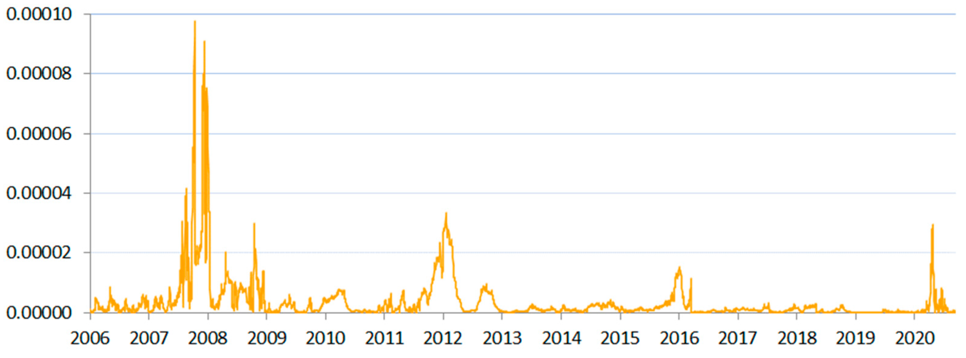
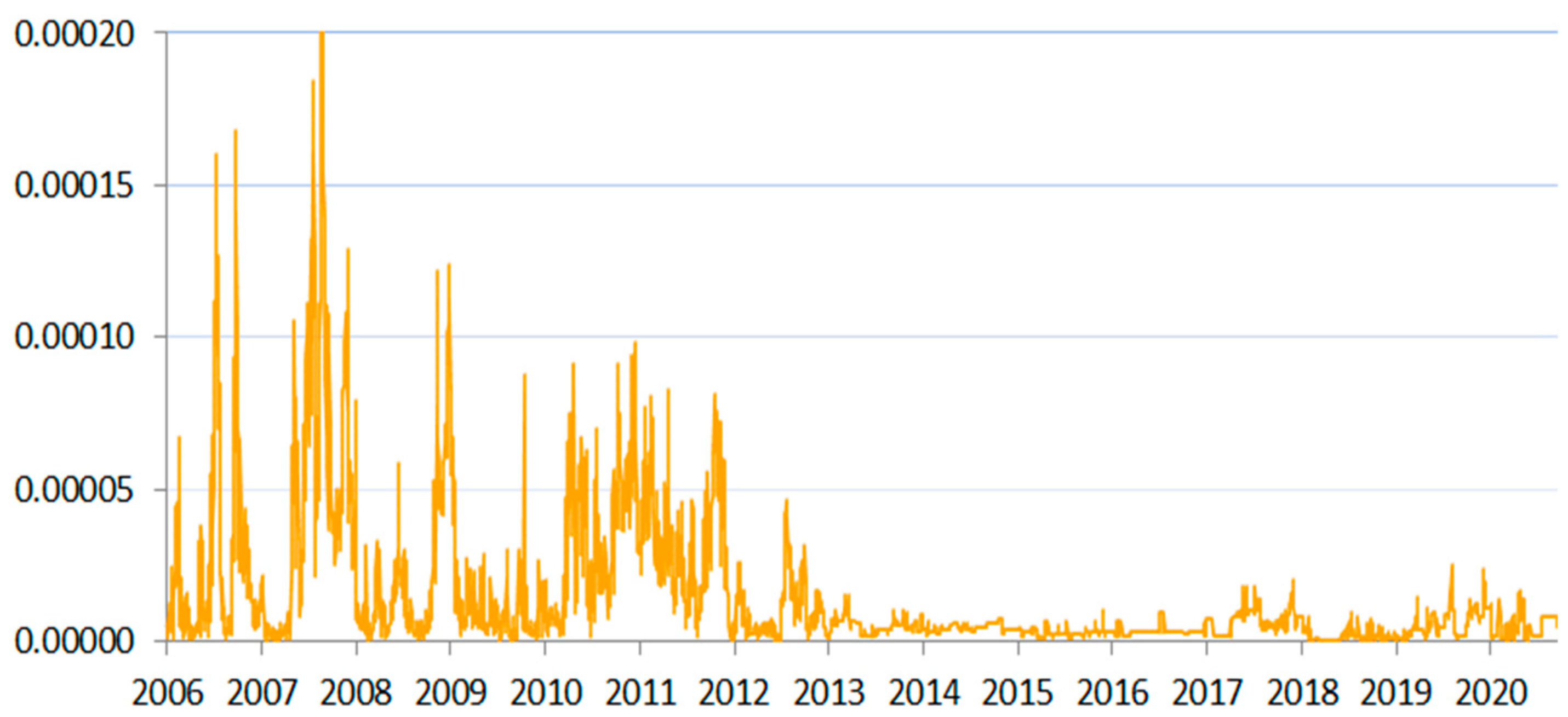
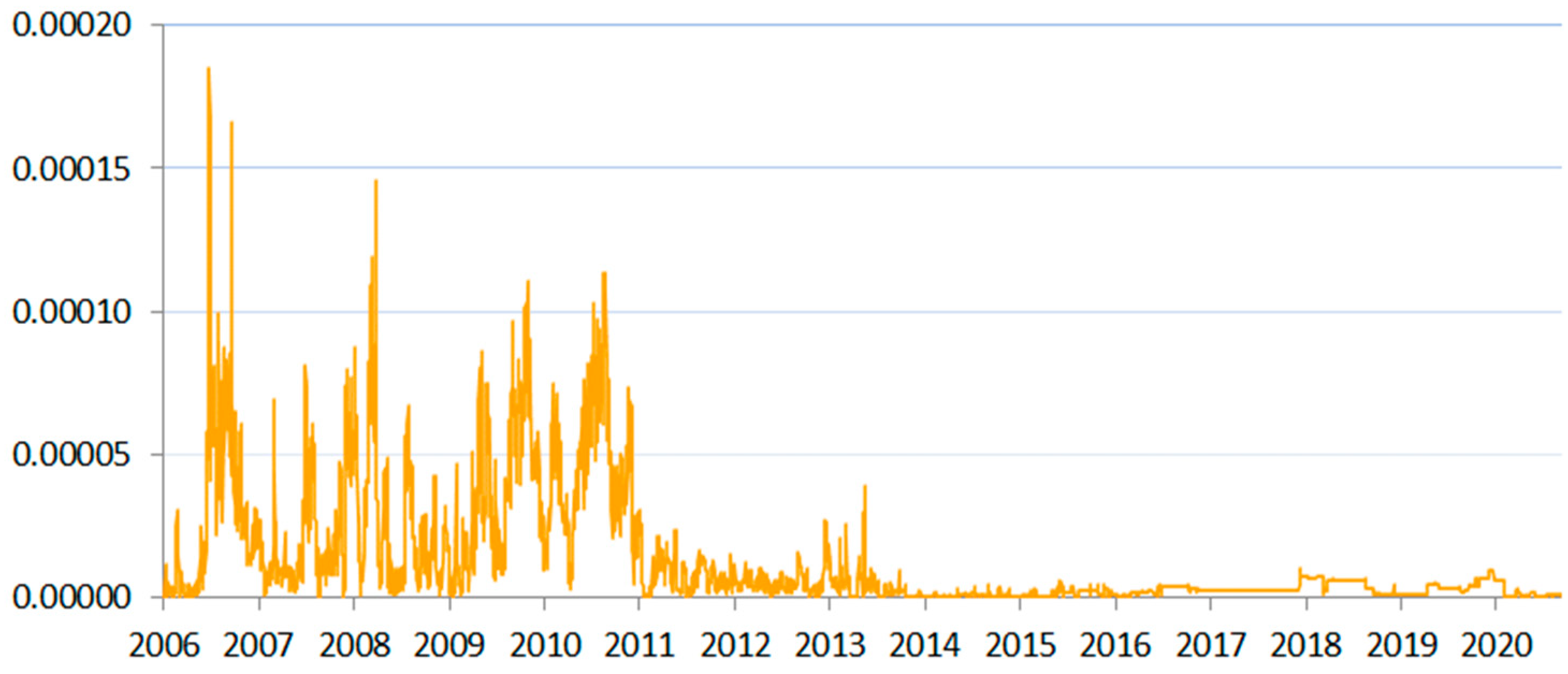
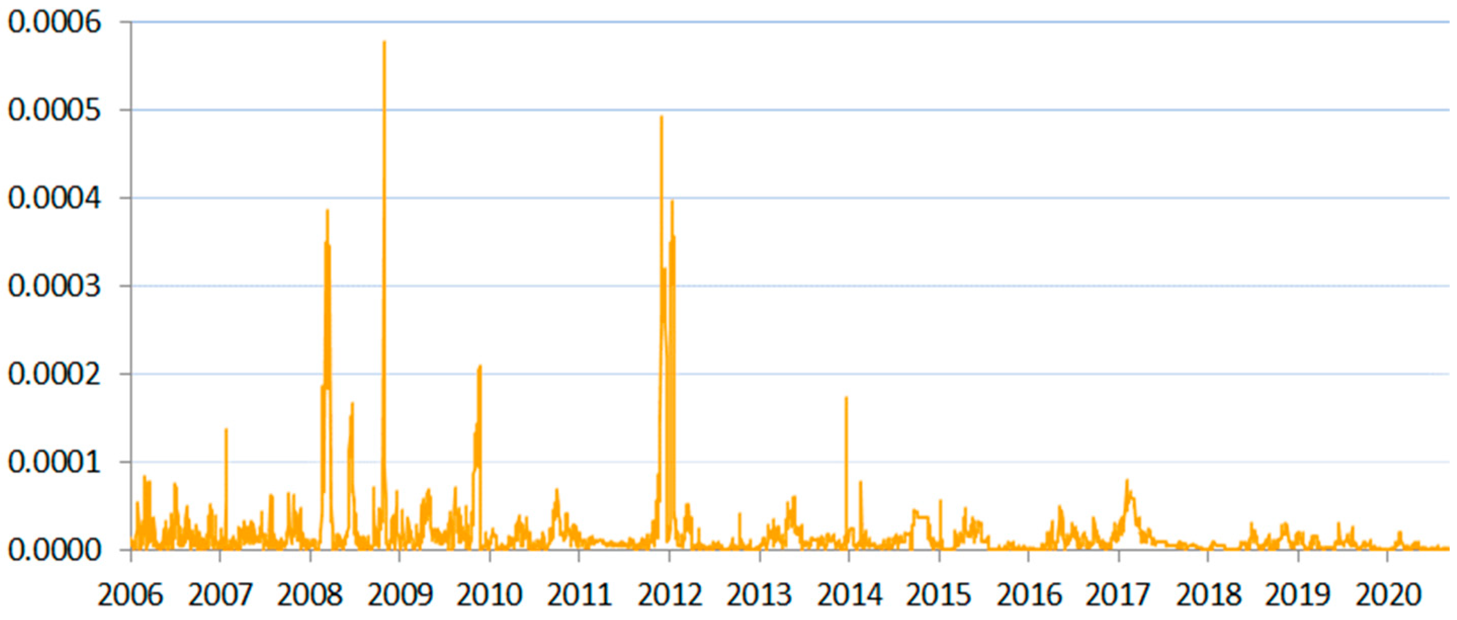
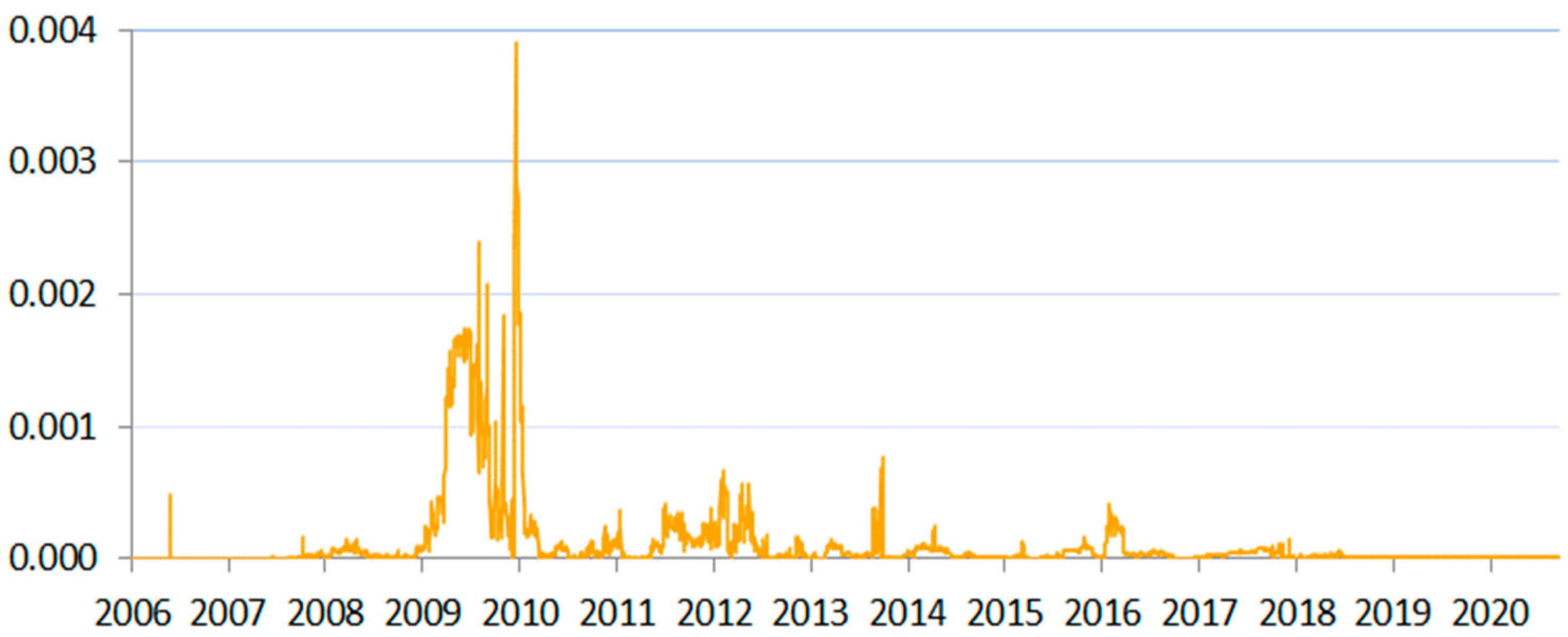
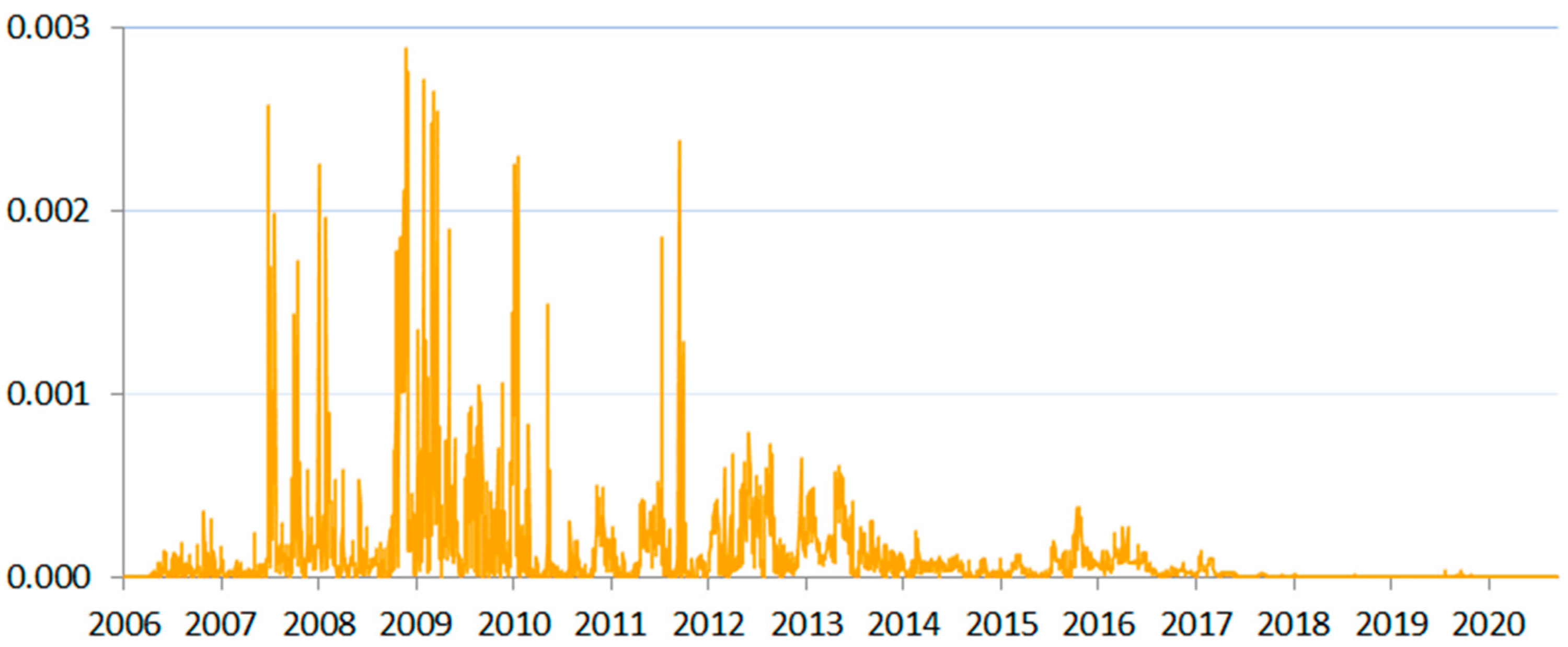
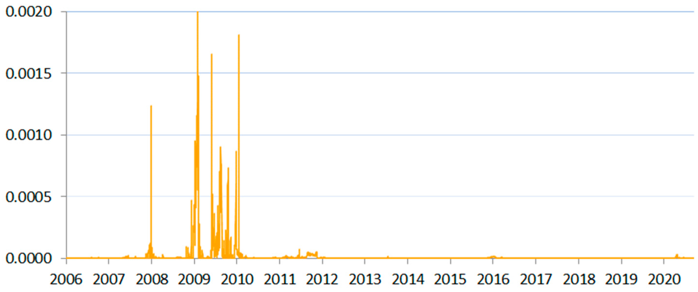
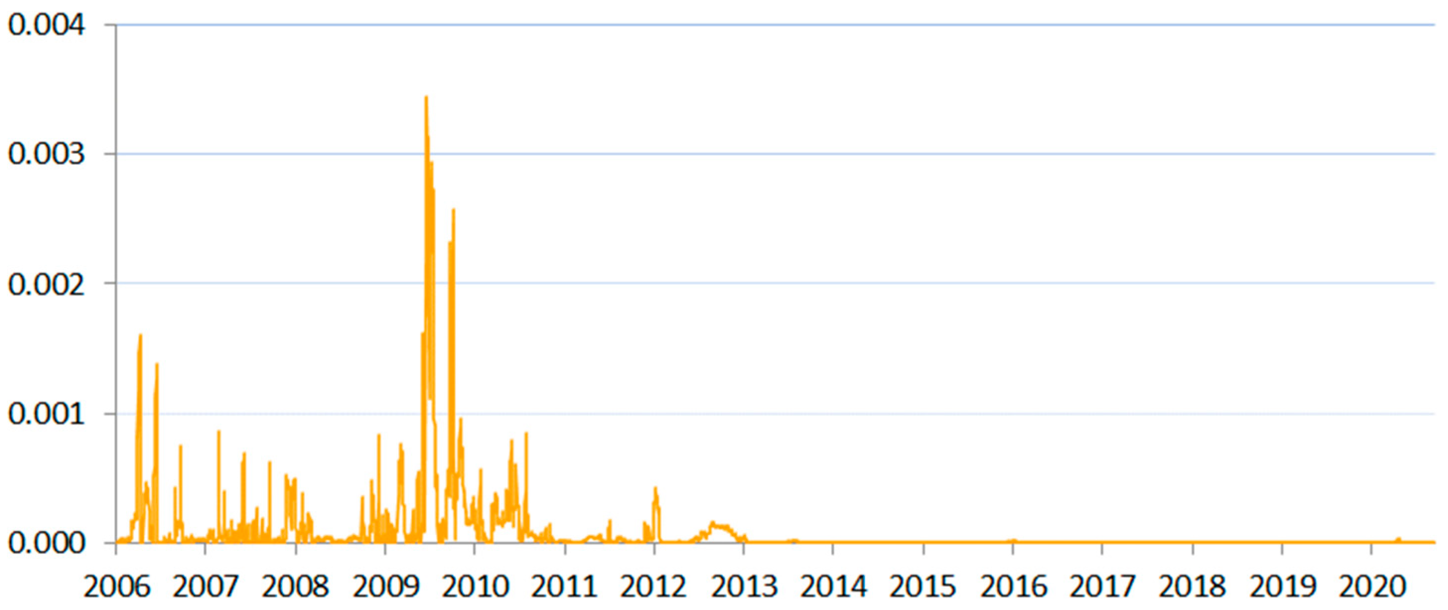
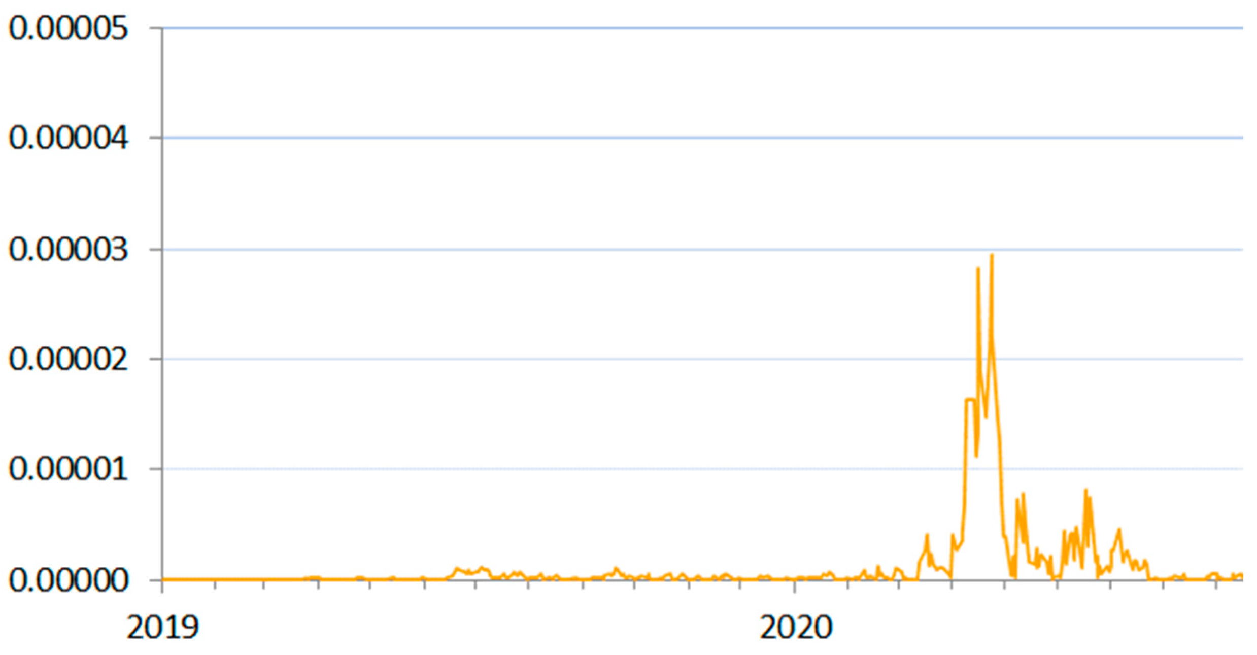
Figure 1, Figure 2, Figure 3, Figure 4, Figure 5, Figure 6, Figure 7, Figure 8, Figure 9 and Figure 10 present the results. Generally, we can say that in all the studied cases, the SIN measure signaled increased risk in two periods between 2007 and early 2010, as well as between late 2010 and 2013. This observation corresponds to the unfolding of the global financial crisis and the sovereign debt crisis in Europe, validating the sensitivity of the SIN measure to the clear-cut financially driven systemic crises in the study period. We also observed a period of increased liquidity risk in the euro area during the ongoing COVID-19 pandemic.
We also observed for all the analyzed markets that following the global financial crisis, liquidity volatility and illiquidity risk gradually fell to comparatively low levels around 2015. At that time, the macroprudential regulations aimed at the elimination of systemic problems from the interbank market were also introduced. The fact that these tools were, to a point, successful is visible in Figure 1, Figure 2, Figure 3, Figure 4, Figure 5, Figure 6, Figure 7, Figure 8, Figure 9 and Figure 10. Although the risk was not eliminated in total, the markets entered the economic crisis caused by the pandemic in a completely different state of liquidity than was the case for the global financial crisis and the public debt crisis. The markets were characterized by a high shock-absorption capacity this time around.
The SIN measure indicated a set of characteristic differences between the studied countries. The differences corresponded to the scale of risk and the specific timing of it. The results also pointed to country-specific periods of higher risk, which seemed to be driven by local events. Below we discuss the results in more detail, separately for the emerging markets and for the frontier markets.
In this study, we analyzed three markets that were classified as emerging during the study period, namely the Czech, Hungarian, and Polish markets. These markets differed quite significantly. Poland had a much bigger market than the other two countries, while the currency risk issues were most pronounced in the Hungarian market, which is in a closer geopolitical proximity to the frontier markets of Bulgaria and Romania. Furthermore, Hungary and Poland had a bigger market share of domestic institutions in the banking sector than Czechia. All of these characteristics were significant for materialization of systemic illiquidity risk. Figure 1, Figure 2 and Figure 3 present the results for the emerging markets.
Poland and Czechia showed very similar risk profiles as far as systemic liquidity was concerned. Given the difference in size of their domestic interbank markets, such a similarity may have resulted from the high convergence with the financial sector of the developed European Union countries. Adequately, we observed high risk in 2010 and 2011, around the time of the European debt crisis, when neither Poland’s nor Czechia’s budgets were significantly hit by it2. We observed a kind of contagion by association with the western EU states. It should be noted that the presence of foreign-owned and foreign-parented banks in the CEE region was a significant contagion channel in such circumstances.
This observation was also in line with the risk peaks in both countries before the global financial crisis (2007), coinciding with the intensification of the liquidity pressures in foreign markets. Czech National Bank (CNB 2008, p. 35) concluded that “market participants behavior [was] over-sensitive or herd-like”, and that market participants were keen to “assign an unhealthy higher weight to market liquidity” in risk assessments, which resulted in severely increased volatility. The composite liquidity indicator calculated by the central bank for that period was at the lowest level since 2000 (see Box 3.1, CNB 2007). On a similar note, Czech National Bank explained the risk in the period between 2010–2011 as caused by the “persisting increased nervousness in the markets” (CNB 2010–2011, p. 40). At that time, the money market was still significantly affected by the recent crisis, as financial institutions were hoarding liquidity in the face of prevailing uncertainty. This constatation also held for Poland and Hungary.
For Czechia, we saw another significant risk peak in 2006. At that time, commercial banks were intensely speculating on the interbank market in the expectation of the increase in the base rates. In response, CNB decreased the frequency of the repo transactions from daily to three weeks. This resulted in even higher volatility that lasted for about four months. Admittedly, the central bank confirmed that its action affected market liquidity negatively (CNB 2007, p. 28).
The Polish interbank market, similar to the other studied markets, was characterized by a decreasing volume of trading, falling volatility of the spreads, and declining differentiation of the interest rates in the period after the financial crisis. However, for Poland, the years 2015–2017 were exceptional in this respect—almost zero volatility and no differentiation of daily quotations of banks participating in fixing were observed. This period was also the time of maintaining constant interest rates by the Monetary Policy Council (Kapuściński and Stanisławska 2017).
In Hungary, we observed several exceptionally high peaks in systemic illiquidity risk. While the increased risk in 2006 and 2014 corresponded to the events described above that were common for all three emerging markets analyzed in this work, it was significantly amplified by domestic events. Among those, we may enumerate currency instability and related problems with entering the euro area, slowdown of the economic growth that stopped the convergence towards the EU’s developed economies, and fiscal problems resulting in fiscal emergency measures (Valentinyi 2012).
Negative market reactions were also observed in relation to various banking tax changes that were introduced between 2014 and 2021, as all of these changes put a strain on the sector, which was much bigger than in other CEE countries. The year 2014 was especially hard for the Hungarian banking sector, as 10 bank collapses took place then. There were media suggestions that this resulted from political decisions related to longer-term vision of the renationalization of the banking sector (Balogh 2015). The most significant closures of banks took place in January and in December of that year.
A vital difference appeared between the Visegrad Group and the rest of the analyzed countries. In Poland, Czechia, Hungary, and Slovakia (Figure 1, Figure 2, Figure 3 and Figure 10), the scale of SIN was one order of magnitude smaller than in other countries. The described scale of risk also corresponded to the relative strength of each local currency. Poland had the most stable local currency among the studied countries, which corresponded to the smallest (other than euro area’s) registered scale of the SIN measure (for comparison, see Figure A1 in Appendix A).
In our study, we also analyzed seven frontier markets. Three of them were developing economies with relatively weak currencies (compared to other European countries): Croatia, Bulgaria and Romania. They were the most aggressively economically developing countries in the sample with the least stable flow of funds from abroad. In addition, for these countries, several domestic crisis-like events may be enumerated (see Kubinschi and Barnea 2016; Andrieş et al. 2018; Barkauskaite et al. 2018; and Karaś and Szczepaniak 2019). It was for these countries that we observed the largest volatility of the SIN measure. Figure 4, Figure 5 and Figure 6 show the results of systemic illiquidity measurements for these frontier markets.
When analyzing the results obtained for Bulgaria (Figure 4), we noticed several periods of systemic illiquidity other than the biggest peak at the time of the global financial crisis. Of special significance was the bank run that took place in 2014. Corporate Commercial Bank AD, which was affected by this run, was the 4th-largest bank in Bulgaria at that time. It had problems already in the late 2012, and it had a negative audit results in mid-2013. The bank’s assets were frozen in June 2014, but no resolution mechanism was put in place immediately. At that time, Bulgaria was in a political crisis, having had five government changes between 2013 and 2014, noting a rise in the deficit from 1.2% to 3.4% and an episode of deflation (BNB 2014). To avoid a bigger financial market run, Bulgaria rescued First Investment Bank, which was reputationally affected by the problems of Corporate Commercial Bank, but was otherwise in a relatively sound condition. This action likely stopped the further contagion effect of the loss of confidence in the banking sector and allowed the restoration of liquidity over time.
Another—much smaller, but still quite significant—peak in liquidity risk was recorded for Bulgaria in 2016. The peak coincided with the increase of conservative prudential liquidity measures for the banking sector. In the financial stability assessment of Bulgaria (IMF 2017, p. 10), we may read that in June 2016, Bulgarian banks had a liquid-assets ratio at a level of 31% (11% above the prudential requirement). In 2020, the liquidity-coverage ratio in the Bulgarian banking sector was at a level of over 260%, much above the regulatory requirements (Radev 2020, p. 1).
The almost flat shape of the SIN measure recorded for the period of the COVID-19 pandemic corresponded to the liquidity-providing operations of the government, including several rescue packages for businesses, as well as the moratorium on deferral of loan repayments possible on the basis of the EU-wide regulatory framework established by the European Banking Authority (EBA) in its guidelines on legislative and nonlegislative moratoria on loan repayments applied in the light of the COVID-19 crisis (EBA 2020).
This EU-wide solution, which affected all the countries analyzed in this paper, has had a positive risk effect in the short term, but is likely to cause delayed negative effects for the financial system in the medium term, when the moratorium expires and loan-performance deterioration will intensify in the region.
Croatia (Figure 5) and Romania (Figure 6) were characterized by high interbank market volatility. One of the major risk factors here was the exchange rate. For instance, Croatia had negative GDP growth in 2010 and 2012, and a major increase in the cost of euro. This coincided with the decrease of the foreign capital inflow, putting further strain on the exchange rate and forcing the Croatian National Bank to take action several times. At that time, the euro interbank market also recorded increased volatility; e.g., the EONIA rate was prone to sudden drops and peaks. Big European banks were sharply deleveraging, while their CDS spreads raised significantly (see Chart 5 in CNB 2012, p. 12). The matter concerned several European banks that had a key presence, inter alia, in Croatia. The coincidence of all of these risk factors was likely responsible for the sizeable peaks in Figure 5. Since 2015, the Croatian banking sector has been noting an improving liquidity position (in 2016, it was the best since 2004—see CNB 2016, p. 48), and this corresponds to the decrease in the levels of the SIN measure.
As far as Romania is concerned, we saw a similar level of volatility that was also driven by, among other factors, the exchange-rate variability. It was further amplified by the fact that many systemically important Romanian banks rely heavily on European parent financing. We also saw the reactions to the same international factors as described for other frontier markets (see, e.g., NBR 2007, p. 7) and the reaction to the European Union accession that put a significant competitive pressure on domestic banks (NBR 2008, p. 72). The intensity of the impact of the external risk factors corresponded to very low liquidity of the interbank market. For instance, in the beginning of the study period, the Romanian interbank market recorded only 200 transactions between October 2005 and February 2007 (NBR 2007, p. 47). Such low liquidity in that time period was a typical trait of all the frontier European markets included in this study. Among more specific Romanian risk factors, we may count a mild liquidity decrease in the first quarter of 2019, when the relatively big bank Bancpost (assets corresponding to 3.3% of the banking sector) was merged into a systemically important bank in Romania—Banca Transilvania S.A. As was the case for other analyzed countries, in Romania we also observed increasing liquidity of banks since 2015. The good liquidity position of the banks was reflected in the low SIN levels in that period.
The final four frontier market countries analyzed in the paper (Estonia, Lithuania, Latvia, and Slovakia) were characterized by more-developed economies and closer economic ties with the European Union. Liquidity risk peaks corresponded in their case to various events in the developed countries that composed the external financial market environment for them (Western EU countries and the Nordic countries). For instance, we could see risk peaks for the Baltics in 2010 that corresponded to liquidity-tightening in the markets in the mentioned countries.
In the periods preceding the euro area entrance, the SIN measure reacted to several domestic events. For instance, in case of Lithuania, we saw a sudden peak by the end of 2008, when the banking sector suffered losses, its loans portfolio was shrinking, and a higher withdrawal of deposits occurred. The peak subsided immediately because “parent banks fully covered liquidity shortage in the market by additional lending to their subsidiaries” (BL 2009, p. 5). Such an occurrence was typical for the Baltic countries, where—in the study period—Northern European parent banks were most willing to intervene to help their subsidiaries.
In Estonia, we saw a big drop in volatility in 2010 in the period when financial institutions were slowly withdrawing from the Estonian interbank market and anticipating Estonia joining the euro area in 2011 (BE 2011). Such a preceding effect also was visible for the other three countries.
Regarding Latvia, in February 2007, Standard & Poor’s lowered the country’s rating forecast from neutral to negative, which hit its currency significantly. The central bank intervened, but the exchange rate remained affected by this event until mid-March. These events also affected the stock exchange and the money market. “The average weighted interest rate on overnight transactions in lats amounted to 4.97% in 2007 (by 177 basis points in excess of the 2006 level). Lats money market rates on longer term transactions also went up, with 6-month RIGIBOR picking up 450 basis points (to 8.98% on average on an annual basis) and 12-month RIGIBOR growing by 453 basis points (to 9.11%) and reaching the maximum in October 2007” (BoL 2007, str. 15). The peaks in Estonia for that period also were related to the turbulence in the Latvian and euro-based interbank markets (BE 2007, p. 47).
On an opposite note, on 23 February 2018, following the money-laundering accusations made by the Financial Crimes Enforcement Network of the United States Department of the Treasury (2018, Federal Register 83/33/Friday), the Financial and Capital Market Commission made a decision on unavailability of deposits at the Latvian ABLV Bank, which was one of the systemically important banks in Latvia at that time. The bank decided on voluntary liquidation. Prompt actions of Latvian regulators allowed the country to avoid a systemic crisis. At the same time, thanks to the fact that Latvia was already in the European interbank market, this domestic event did not affect systemic liquidity. The depth of the European market was large enough to dissipate any related shocks (BoL 2019) A similar case involved the Estonian branch of Danske Bank, which entered into liquidation in August 2018, after a money-laundering3 scandal in early 2018. In this case, no significant market freeze was reported as well. The SIN measure reacted accordingly in both cases—no significant peaks were recorded.
Of special note was the shape of the time series indicative of systemic liquidity in the Baltics and Slovakia. Here, we saw sharp but relatively short liquidity declines. For the rest of the time, the indicator remained very low, suggesting stability. We also saw significant overlap in systemic conditions for the Baltic countries, showing that the region was the most convergent among the analyzed states. This pointed to a higher risk of illiquidity-driven contagion in the Baltics. Such observations were in line with the fact that Estonia, Lithuania, and Latvia only have a small number of systemically important banks, all of which strongly depend on the same financing from Sweden and Norway.
The Baltic countries and Slovakia adopted the euro currency in the study period (2009, 2011, 2014, and 2015, respectively), which changed their foreign-exchange-rate risk profile. Figure 7, Figure 8, Figure 9 and Figure 10 show how the accession changed the depth of their interbank market, increasing liquidity and lowering volatility very significantly, as these countries turned from small-scale, local-rate-based wholesale funding to euro-area funding.
4.3. COVID-19 Pandemic
In the postcrisis period and before the COVID-19 pandemic, when ample liquidity still remained in the financial system—a remnant of the quantitative easing and prolonging negative interest rates—systemic illiquidity risk was minimal. The results suggested that the scale of risk in the interbank market has gone down. Nevertheless, one cannot be certain that this change is a permanent one. In fact, one may also argue that the risk was not mitigated, but simply shifted to the shadow-banking sector (ECB 2020).
The direction of the diffusion of the COVID-19 crisis varied from the systemic shocks observed before. Compared to the crisis in 2007–2010, when the shock originated in the financial sector and then spilled over to the real economy, the COVID-19 pandemic spread oppositely: first, the real economy was affected, then the spillover to the financial sector followed (BIS 2020).
For less-developed countries of the EME region, the COVID-19 pandemic mainly caused shocks in capital flows that influenced currency exchange rates, causing the depreciation of local currencies (FSB 2020). Central banks started to offer foreign-exchange operations to stabilize the exchange-rate volatility, and immediately announced liquidity support to protect the financial system against any disruptions (IOSC 2020). In the CEE region, the central banks of Hungary, Poland, and Romania purchased government securities in secondary markets to restore their liquidity and strengthen the mechanism of monetary-policy transmission (Cantú et al. 2021, p. 15). Among other actions, the central banks implemented reserve policy changes to quickly free up liquidity and established nontargeted lending operations in the first months of the pandemic (Cantú et al. 2021, p. 11). The immediate intervention of the central banks, which supported the process of market running, enabled them to minimize negative consequences of the pandemic for the financial sector in the study period. This was depicted by the low levels of the SIN measure.
In the euro area, the situation in the interbank market was quite different. “While the core of the financial system—including major banks and financial infrastructures—entered the crisis more resilient than in the run-up to the global financial crisis, the COVID-19 shock led to severe liquidity stress in the system” (BIS 2021, p. 3). Described liquidity shocks were recorded by the SIN measure (Figure 11). They were short and took place at the beginning of the COVID-19 pandemic.
In March 2020, asset markets froze in many countries. The growing cash needs resulted in the widening of spreads on fixed-income instruments, the yields (mainly long-term) of which increased significantly (Schrimpf et al. 2020; Hördahl and Shim 2020). The situation was observed mainly in the developed markets in Europe—especially in the euro area, where the outflow from money market funds reflected sudden liquidity needs (IOSC 2020). Investors tried to move from the more-liquid, but also riskier, sector (various asset classes) into a less-sensitive one (sovereign bonds).
The situation stabilized very quickly (by the end of March in the euro market) thanks to the immediate and synchronized reaction of the central banks. ECB announced and implemented several supportive actions: the temporary capital and operational relief in reaction to coronavirus (12 March 2020), the temporary pandemic emergency purchase program (18 March 2020) and a package of collateral easing measures (7 April and 22 April 2020) (EBA 2020). Our results confirmed that for the time being, these measures alleviated systemic risk in the financial system.
One should bear in mind that the illiquidity and the effects of the COVID-19 pandemic may be delayed in time because of the financial help from euro-area governments that basically poured liquidity directly into the system, a series of actions that in this respect resembles quantitative easing (see Christensen and Gillan 2014). It will thus certainly be interesting to see how the SIN measure behaves in the upcoming months and in a longer period of two or more years, when the economic downturn that started with the pandemic will put most of the strain on systemic risk. The longer-term effects of the help packages will most definitely be significant, and it is difficult to say with certainty what adverse effects will follow.
Nonetheless, at least three facts are certain. Governments are running unprecedented deficits and public debt has been building up fast, also in the face of the locked-down economy. In the past, the public debt buildup resulted in the increase of systemic illiquidity risk, among other things. This time, the inflation effects are also uncertain, as the monetary policy interest-rate channel working through the interbank market is almost nonexistent, with historically low base rates across the region.
Secondly, the issues of moral hazard are clear. The large-scale support measures introduced recently “may induce moral hazard, causing investors to underestimate market risk [and] infer that liquidity support will always be provided” (BIS 2021, p.18), which will cause systematic mispricing of the market liquidity risk.
Thirdly, many central banks have had deteriorated balance sheets ever since the global financial crisis, which was the effect of the previous unprecedented activities to stabilize the financial system, such as direct quantitative easing and buying back bad collateral from the banking sector. Now, “The need to intervene in such a substantial way has meant that central banks had to take on material financial risk” (BIS 2021, p. 2). It is impossible to say how this will affect their stability in the longer run and what the exit strategy is at this point.
From a global perspective, we are facing unprecedented uncertainty in any economic and financial aspect that exists. The effects of the current events are so unpredictable for one reason: namely, the entire global economy and the entire global financial sector is being affected by the same crisis at once. It is no longer the case of one market problem spilling over to the rest of the world—this time the shock is simultaneous everywhere. There are questions regarding whether the rescue measures will be able to outlast the pandemic until it subsides for good, and what will happen when the support measures start to be phased out.
5. Conclusions
In the course of this paper, we discussed the role of liquidity and its imbalances in systemic risk materialization, and we overviewed the results of existing systemic illiquidity-focused theoretical and empirical research. This literature review showed how important liquidity measurement and monitoring are in systemic risk analysis. Next, we discussed the applicability of the existing methods of systemic liquidity measurement to the CEE region. We concluded that these methods were inapplicable to the frontier and emerging financial markets under our analysis, and therefore a new approach is necessary to measure systemic liquidity risk for the given set of countries.
This conclusion also held for many other less-developed financial markets in the world that are characterized by the same specificity as the countries analyzed by us. In this way, we found an existing research gap in systemic liquidity analysis that relates to countries with frontier and emerging markets.
To fill the gap, we developed a new approach to illiquidity risk measurement using the interbank market data and Nelson–Siegel–Svensson methodology. Our measure—the Systemic Illiquidity Noise (SIN)-based measure—was empirically applied to a selected set of 10 CEE countries. In this way, we obtained the results of systemic illiquidity analysis for seven frontier and three emerging financial markets, for which such analysis was impossible before.
The empirical results displayed a successful application of the proposed method. The SIN measure proved to be sensitive to the global liquidity breakdown that took place during the global financial crisis and the European debt crisis. Similarly, the measure was reactive at times of locally important systemic events, such as runs on banks or periods of significant currency depreciation in different countries. Moreover, SIN facilitated identifying three divergent sets of countries with different systemic liquidity risk characteristics.
The results also captured the impact of introducing the euro currency on systemic liquidity risk. For the example of the euro area, we also showed that the SIN measure reacted to a liquidity shock caused by the current pandemic. This was despite the fact that the financial sector was very liquid before the shock. In effect, we may conclude that the SIN measure was sensitive to systemic liquidity shocks of different origins and magnitudes, regardless of the prevailing levels of liquidity per se.
There were at least two significant advantages to the methodology developed in the course of this study. First, the SIN measure allowed for contemporaneous monitoring of systemic liquidity at a minimal cost—using well-known models and easily accessible data. This is of potential high value to any frontier or emerging market regulator and supervisor, as such monitoring may be easily introduced and sustained, giving macroprudential bodies a better chance to react to future financial crises and to mitigate potential costs of such crises.
Second, although the study encompassed only 10 selected countries, given their diversity and the stability of our results, there is a potential for the successful application of our method to other markets, as long as there is a continuous interbank market there. Although the Interbank Offered Rates were used in this study, other similar types of rates also would be feasible, regardless of their fixing methodology. Such a potential of broad application of our measure creates an opportunity for a better and increased understanding of systemic liquidity disturbances on an international scale, regardless of the level of financial market development in each specific country.
Finally, this study is of pragmatic value not only to regulators, but also to other participants in the financial system, especially banks, because they may also use the SIN measure to monitor the systemic liquidity risk that affects them so significantly. Better-informed regulators and financial market participants would be better-equipped to make better risk management decisions, which in the long run might add to lowering systemic risk in the financial system as a whole.
Author Contributions
Conceptualization, M.A.K. and E.D.; Data curation, E.D.; Formal analysis, M.A.K. and E.D.; Funding acquisition, M.A.K.; Investigation, M.A.K. and E.D.; Methodology, M.A.K. and E.D.; Project administration, M.A.K.; Software, E.D.; Validation, M.A.K. and E.D.; Visualization, E.D.; Writing—original draft, M.A.K. and E.D.; Writing—review & editing, M.A.K. and E.D. All authors have read and agreed to the published version of the manuscript.
Funding
This research project was funded by the National Science Centre under Agreement UMO-2018/29/N/HS4/02783.
Conflicts of Interest
The authors declare no conflict of interest.
Appendix A
Figure A1.
Systemic Illiquidity Noise-based measure calculated for the euro area.
Appendix B

Table A1.
Measures focused on illiquidity applicable to systemic-scale analysis.
| Measurement Output | Authors | Short Description |
|---|---|---|
| Liquidity factor | Pastor and Stambaugh (2003) | A measure of market liquidity computed as the equally weighted average of the liquidity measures of individual stocks, using daily data. Specifically, the liquidity measure for a stock is the ordinary least squares regressed function of quantities of the daily returns on this stock in a given month, its volume, and the value-weighted market return. The measure relies on the principle that order flow induces greater return reversals when liquidity is lower, viewing volume-related return reversals as arising from liquidity effects. |
| A set of interpretable parameters | Getmansky et al. (2004) | The proposal to use autocorrelation of returns of hedge funds as a proxy of their liquidity; the first-, second-, and third-order autocorrelations for each hedge fund’s returns are computed using an econometric model of return smoothing coefficients and used as a proxy for quantifying illiquidity exposure—the less liquid the fund, the more serial correlation is observed. |
| Broader hedge-fund-based systemic risk measures | Chan et al. (2006) | A set of three measures quantifying the hedge funds’ impact on systemic risk by examining the risk/return profiles of hedge funds, using returns and sizes data, at the individual and aggregate levels in relation to the investment risk they bear: autocorrelation-based measure of illiquidity exposures, a liquidation probability-based measure, and the regime-switching-based model quantifying the aggregate distress level in the hedge fund sector. |
| Five measures of contagion potential | Billio et al. (2012) | A structured approach to measure systemic risk with indicators based on illiquidity (quantified by autocorrelation) and correlation, using principal component analysis (indicating the degree of assets commonality), regimeswitching models, Granger causality tests (indicating the direction of propagation of systemic triggers), and network diagrams (visualizing the connectedness via directional networks), focused on detecting of interdependence between banks, brokers, insurers, and hedge funds, based on statistical relations among their market returns. This way, the authors quantify the potential contagion effects in the analyzed financial system. |
| A system of liquidity risk charges (LRCs) | Perotti and Suarez (2011) | Pigouvian charges are calculated per unit of refinancing risk-weighted liabilities based on a vector of additional systemic factors (such as size and interconnectedness) in a given period. The weighting function is decreasing and smooth to avoid regulatory arbitrage, which could distort market rates. The model is aimed at making banks internalize negative systemic effects of fragile funding strategies, but the computed size of charges may be used as a tool for quantifying liquidity risk showing which institutions generate more risk for the financial system. |
| Contrarian strategy liquidity measure (CSL) | Khandani and Lo (2011) | A proposal to apply mean-reversion equity market strategy (buying losers and selling winners over 5 to 60 min lagged returns) to proxy the market-making (i.e., liquidity-provisioning) profits and to obtain equity market liquidity measure by observing the performance of this trading strategy. The authors showed that when it does very well, there is less liquidity in the market, and vice versa. |
| Price-impact liquidity measure (PIL) | An inverse proxy of liquidity, in which liquidity is measured with a linear-regression estimate of the volume required to move the price of a security by one dollar; i.e., higher values of lambda imply lower liquidity and market depth. The aggregate measure of market liquidity (PIL) is computed as the daily cross-sectional average of the estimated price-impact coefficients. | |
| Systemic Liquidity Risk Index (SLRI) | Severo (2012) | The SLRI is calculated by integrating the deviations of the following basis spreads: covered interest parity, the on-the-run versus the off-the-run interest-rate spread on government bonds, and the interest-rate spread between the overnight index swap (OIS) and short-term government bonds and the CDS basis spread, to represent the degree of their comovement first component score from a principal component analysis (based on historical time-series data) is used. |
| Liquidity Mismatch Index (LMI) | Brunnermeier et al. (2014) | Measures the difference between the cash-equivalent future values of the assets and liabilities of a bank; it utilizes the cash-equivalent value, which is the product of the asset or liability current value, multiplied by the liquidity weight (positive for assets, negative for liabilities), which depends on an assumed stress scenario, Value-at-Liquidity-Risk, defined as the quantile of worst losses (e.g., 5%), and the Expected Liquidity Loss, which corresponds to the average of the liquidity losses beyond this threshold. The authors proposed to use LMI to identify the most systemically important financial institutions. |
| Systemic risk-adjusted liquidity (SRL) model | Jobst (2014) | Estimates the probability and severity of joint liquidity events; i.e., instances of banks jointly breaching their Net Stable Funding Ratios. Estimation process: 1. The components of the NSFR are valued at market prices in order to generate a time-varying measure of funding risk relative to prudential liquidity standards. 2. Aggregate cash flow implications of changes to liquidity risk are modeled as a put option to estimate losses expected from insufficient stable funding. 3. Individually estimated liquidity risk net exposures are aggregated via a multivariate distribution to determine the probabilistic measure of joint liquidity shortfalls on a system-wide level. |
| Systemicness | Greenwood et al. (2015) | A linear model of fire-sale-induced liquidity crises, computing banks’ equity shock exposures to system-wide deleveraging and to spillovers induced by individual banks; systemicness is a (quantity) measure of a bank’s contribution to financial sector fragility, proportional to its size, leverage, and connectedness (owning large and illiquid asset classes to which other banks are also highly exposed).The key assumption is that banks target a given level of leverage, and this implies asset sales when leverage grows beyond the target. It allows the measurement of how the distribution of banks’ leverage and risk exposures contributes to systemic risk. |
| Cumulative Distance to Default (CDD) | Karkowska (2015) | The distance-to-default measure is a market-based measure of credit risk based on Merton’s model, in which the equity of a firm is modeled as a call option on the value of its assets. The exercise price is equal to the value of the liabilities (the firm defaults when its assets’ value falls below its debt face value). For implementation, the face value of debt is assumed to be equal to the sum of short-term liabilities and half the long-term liabilities from the balance-sheet data. The model is calibrated using the analyzed institution’s market value and its equity price volatility. Karkowska used this method to derive the DD value for each institution forming the studied banking system and aggregated the data to obtain a systemic risk measure equal to the total probability of default of all the studied institutions. |
| Aggregate vulnerability (AV) and illiquidity concentration | Duarte and Eisenbach (2019) | An extension of the systemicness measure that includes the panel analysis tracking vulnerabilities over time. It takes banks’ leverage, asset holdings, asset liquidation behavior, and the price impact of liquidating assets in the secondary market as given, and models banks’ responses to negative liquidity shocks (fire-sale spillovers); using information embedded in repo haircuts to account for changes in asset-specific liquidity and flow-of-funds data, it allows to measure aggregate liquidity, defined as the sum of all the second-round spillover losses (not the initial direct losses) as a share of the total equity capital in the system; the factors’ decomposition applied produces a new component of AV, namely illiquidity concentration. The authors showed that the measure Granger-causes most other systemic risk measures. |
The table presents all the complex measures applicable to systemic risk analysis focused on illiquidity considered in the study. For each method or measure, we provide a short description of the mechanism behind the measurement output.
| 1 | Countries were classified according to the criteria of the S&P DJI’s Global Benchmark Index for the study period. |
| 2 | Poland instigated the emergency mechanism to limit public debt in 2014, when the debt was at 56% of GDP. |
| 3 | In that period, several cases of monely laundering were reported in the CEE region, including ABLV bank (Latvia), Danske Bank (Estonia), Versobank (Estonia), and other smaller banks in the Baltics. |
References
- Acharya, Viral V., and Ouarda Merrouche. 2013. Precautionary Hoarding of Liquidity and Interbank Markets: Evidence from the Subprime Crisis. Review of Finance 17: 107–60. [Google Scholar] [CrossRef]
- Acharya, Viral V., Douglas Gale, and Tanju Yorulmazer. 2011. Rollover Risk and Market Freezes. The Journal of Finance 66: 1177–209. [Google Scholar] [CrossRef] [Green Version]
- Afonso, Gara, Anna Kovner, and Antoinette Schoar. 2011. Stressed, Not Frozen: The Federal Funds Market in the Financial Crisis. Staff Report 437. New York: Federal Reserve Bank. [Google Scholar]
- Allen, Franklin, and Douglas Gale. 1994. Limited Market Participation and Volatility of Asset Prices. The American Economic Review 84: 933–55. [Google Scholar]
- Allen, Franklin, and Douglas Gale. 2000a. Bubbles and Crises. The Economic Journal 110: 236–55. [Google Scholar] [CrossRef]
- Allen, Franklin, and Douglas Gale. 2000b. Financial Contagion. Journal of Political Economy 108: 1–33. [Google Scholar] [CrossRef]
- Allen, Franklin, Elena Carletti, and Douglas Gale. 2009. Interbank market liquidity and central bank intervention. Journal of Monetary Economics 56: 639–52. [Google Scholar] [CrossRef] [Green Version]
- Andrieş, Alin Marius, Simona Nistor, and Nicu Sprincean. 2018. The impact of central bank transparency on systemic risk—Evidence from Central and Eastern Europe. Research in International Business and Finance 51: 100921. [Google Scholar] [CrossRef]
- Aragon, George, and Philip Strahan. 2009. Hedge Funds as Liquidity Providers: Evidence from the Lehman Bankruptcy. Working Paper 15336. Cambridge: National Bureau of Economic Research. [Google Scholar]
- Balogh, Eva S. 2015. Ten Hungarian Banks Failed Within One Year. Hungarian Spectrum, March 4. [Google Scholar]
- Banerjee, Ryan N., and Hitoshi Mio. 2014. The Impact of Liquidity Regulation on Banks. BIS Working Papers 470. Basel: Bank for International Settlements. [Google Scholar]
- Bank for International Settlements (BIS). 2005. Zero-Coupon Yield Curves: Technical Documentation. BIS Paper No 25. Basel: Monetary and Economic Department, Bank for International Settlements. [Google Scholar]
- Bank for International Settlements (BIS). 2020. A Global Sudden Stop. Chapter 1 and Chapter 2, Annual Economic Report 2020. Basel: Bank for International Settlements. [Google Scholar]
- Bank for International Settlements (BIS). 2021. COVID-19 Support Measures. Extending, Amending and Ending. April 6. Available online: https://www.fsb.org/wp-content/uploads/P060421-2.pdf (accessed on 23 March 2021).
- Bank of Estonia (BE). 2007. Financial Stability Review 2/2007. Available online: https://www.eestipank.ee/en/publications/series/financial-stability-review (accessed on 23 March 2021).
- Bank of Estonia (BE). 2011. Financial Stability Review 2/2011. Available online: https://www.eestipank.ee/en/publications/series/financial-stability-review (accessed on 23 March 2021).
- Bank of Latvia (BoL). 2007. Financial Stability Report. Available online: https://www.bank.lv/en/publications-r/financial-stability-report (accessed on 23 March 2021).
- Bank of Latvia (BoL). 2019. Financial Stability Report. Available online: https://www.bank.lv/en/publications-r/financial-stability-report (accessed on 23 March 2021).
- Bank of Lithuania (BL). 2009. Financial Stability Review. Available online: https://www.lb.lt/en/ch-publications/category.39/series.169#group-2 (accessed on 23 March 2021).
- Barkauskaite, Aida, Ausrine Lakstutiene, and Justyna Witkowska. 2018. Measurement of Systemic Risk in a Common European Union Risk-Based Deposit Insurance System: Formal Necessity or Value-Adding Process? Risks 6: 137. [Google Scholar] [CrossRef] [Green Version]
- Berg, Andrew, and Catherine Pattillo. 1999. Are Currency Crises Predictable? A Test. IMF Staff Papers 46: 108–38. [Google Scholar]
- Bessembinder, Hendrik, Jia Hao, and Michael L. Lemmon. 2011. Why Designate Market Makers? Affirmative Obligations and Market Quality. Working Paper. Washington, DC: International Monetary Fund. [Google Scholar]
- Bhattacharya, Sudipto, and Douglas Gale. 1987. Preference shocks, liquidity and central bank policy. In New Approaches to Monetary Economics. Edited by William Barnett and Kenneth Singleton. New York: Cambridge University Press, pp. 69–88. [Google Scholar]
- Billio, Monica, Mila Getmansky, Andrew W. Lo, and Loriana Pelizzon. 2012. Econometric measures of connectedness and systemic risk in the finance and insurance sectors. Journal of Financial Economics 104: 535–59. [Google Scholar] [CrossRef]
- Blåvarg, Martin, and Patrick Nimander. 2002. Interbank Exposures and Systemic Risk. Sveriges Riksbank’s Economic Review 2: 19–45. [Google Scholar]
- Boss, Michael, Helmut Elsinger, Martin Summer, and Stefan Thurner. 2004. Network topology of the interbank market. Quantitative Finance 4: 677–84. [Google Scholar] [CrossRef]
- Boyson, Nicole M., Christof W. Stahel, and Rene M. Stulz. 2010. Hedge Fund Contagion and Liquidity Shocks. Journal of Finance 65: 1789–816. [Google Scholar] [CrossRef]
- Brunnermeier, Markus K. 2008. Bubbles. In New Palgrave Dictionary of Economics. Edited by Lawrence E. Blume and Steven Durlauf. London: Palgrave Macmillan. [Google Scholar]
- Brunnermeier, Markus K., and Lasse H. Pedersen. 2009. Market Liquidity and Funding Liquidity. Review of Financial Studies 22: 2201–38. [Google Scholar] [CrossRef] [Green Version]
- Brunnermeier, Markus K., and Martin Oehmke. 2013. The Maturity Rat Race. The Journal of Finance 68: 483–521. [Google Scholar] [CrossRef]
- Brunnermeier, Markus K., and Yuliy Sannikov. 2014. A Macroeconomic Model with a Financial Sector. The American Economic Review 104: 379–421. [Google Scholar] [CrossRef] [Green Version]
- Brunnermeier, Markus K., Gary Gorton, and Arvind Krishnamurthy. 2014. Liquidity Mismatch Measurement. In Risk Topography: Systemic Risk and Macro Modeling. NBER Chapters. Cambridge: National Bureau of Economic Research, pp. 99–112. [Google Scholar]
- Brunnermeier, Markus K., Thomas M. Eisenbach, and Yuliy Sannikov. 2013. Macroeconomics with Financial Frictions: A Survey. In Advances in Economics and Econometrics, Tenth World Congress of the Econometric Society. New York: Cambridge University Press, vol. 2, pp. 3–96. [Google Scholar]
- Buiter, Willem Hendrik. 2008. Central Banks and Financial Crises. London School of Economics and Political Science Discussion Paper 619. Financial Markets Group. London: London School of Economics and Political Science. [Google Scholar]
- Bulgarian National Bank (BNB). 2014. Economic Review. April. Available online: https://www.bnb.bg/bnbweb/groups/public/documents/bnb_publication/pub_ec_r_2014_04_en.pdf (accessed on 23 March 2021).
- Caballero, Ricardo, and Alp Simsek. 2013. Fire Sales in a Model of Complexity. The Journal of Finance 68: 2549–87. [Google Scholar] [CrossRef] [Green Version]
- Cantú, Carlos, Paolo Cavallino, Fiorella De Fiore, and James Yetman. 2021. A Global Database on Central Banks’ Monetary Responses to Covid-19. BIS Working Papers 934. Basel: Bank for International Settlements. [Google Scholar]
- Cespa, Giovanni, and Thierry Foucault. 2014. Illiquidity Contagion and Liquidity Crashes. Review of Financial Studies 27: 1615–60. [Google Scholar] [CrossRef] [Green Version]
- Chan, Nicholas, Mila Getmansky, Shane M. Haas, and Andrew W. Lo. 2006. Do Hedge Funds Increase Systemic Risk? Federal Reserve Bank of Atlanta Economic Review 91: 49–80. [Google Scholar]
- Chan-Lau, Jorge A., Marco Espinosa, and Juan Sole. 2009. On the Use of Network Analysis to Assess Systemic Financial Linkages. Global Financial Stability Report. Washington, DC: International Monetary Fund. [Google Scholar]
- Choudhry, Moorad. 2018. An Introduction to Banking: Principles, Strategy and Risk Management (Securities Institute), 2nd ed. Chichester: John Wiley & Sons, Ltd. [Google Scholar]
- Christensen, Jens H., and James M. Gillan. 2014. Does Quantitative Easing Affect Market Liquidity? Federal Reserve Bank of San Francisco Working Paper 2013-26. Available online: https://www.frbsf.org/economic-research/publications/working-papers/2013/26/ (accessed on 12 February 2021).
- Cifuentes, Rodrigo, Hyun Shin, and G. ianluigi Ferrucci. 2005. Liquidity Risk and Contagion. Journal of the European Economic Association 3: 556–66. [Google Scholar] [CrossRef]
- Clementi, David. 2001. Financial Markets: Implications for Financial Stability. Balance Sheet 9: 7–12. [Google Scholar] [CrossRef]
- Coval, Joshua D., and Erik Stafford. 2007. Asset Fire Sales (and Purchases) in Equity Markets. Journal of Financial Economics 86: 479–512. [Google Scholar] [CrossRef] [Green Version]
- Cox, John C., Jonathan Ingersoll, and Stephen Ross. 1981. The relation between forward prices and futures prices. Journal of Financial Economics 9: 321–46. [Google Scholar] [CrossRef]
- Czech National Bank (CNB). 2007. Financial Stability Report. Available online: https://www.cnb.cz/en/financial-stability/fs-reports/ (accessed on 23 March 2021).
- Czech National Bank (CNB). 2008. Financial Stability Report. Available online: https://www.cnb.cz/en/financial-stability/fs-reports/ (accessed on 23 March 2021).
- Czech National Bank (CNB). 2010–2011. Financial Stability Report. Available online: https://www.cnb.cz/en/financial-stability/fs-reports/ (accessed on 23 March 2021).
- Czech National Bank (CNB). 2012. Financial Stability Report. Available online: https://www.cnb.cz/en/financial-stability/fs-reports/ (accessed on 23 March 2021).
- Croatian National Bank (CNB). 2016. Financial Stability, No. 17. Available online: https://www.hnb.hr/en/-/financial-stability-17 (accessed on 23 March 2021).
- de La Grandville, Olivier. 2001. Bond Pricing and Portfolio Analysis. Cambridge and London: MIT Press. [Google Scholar]
- Diamond, Douglas W., and Raghuram G. Rajan. 2005. Liquidity Shortages and Banking Crises. Journal of Finance 60: 615–47. [Google Scholar] [CrossRef] [Green Version]
- Drehmann, Mathias, and Nikola Tarashev. 2011. Systemic Importance: Some Simple Indicators. BIS Quarterly Review. Available online: https://ssrn.com/abstract=1785264 (accessed on 12 February 2021).
- Duarte, Fernando, and Thomas Eisenbach. 2019. Fire-Sale Spillovers and Systemic Risk. Staff Report 645. New York: Federal Reserve Bank. [Google Scholar]
- Duffie, Darrell. 2020. Still the World’s Safe Haven? Redesigning the U.S. Treasury Market after the COVID-19 Crisis. Hutchins Center Working Papers No 62. June. Available online: https://www.brookings.edu/research/still-the-worlds-safe-haven/ (accessed on 25 March 2021).
- Dziwok, Ewa. 2017. Chosen measures for pricing of liquidity. In Contemporary Trends and Challenges in Finance. Edited by Krzysztof Jajuga, Lucjan Orlowski and Karsten Staehr. Springer Proceedings in Business and Economics. Cham: Springer, pp. 3–9. [Google Scholar]
- EIOPA. 2016. Financial Stability Report, EIOPA-FSI-16-016. Frankfurt am Main: European Insurance and Occupational Pensions Authority. [Google Scholar]
- EIOPA. 2017. Technical Documentation of the Methodology to Derive EIOPA’s Risk-Free Interest Rate Term Structures. EIOPA-BoS-15/035. January 30, Frankfurt am Main: European Insurance and Occupational Pensions Authority. [Google Scholar]
- Elsinger, Helmut, Alfred Lehar, and Martin Summer. 2006. Risk Assessment for Banking Systems. Management Science 52: 1301–14. [Google Scholar] [CrossRef] [Green Version]
- European Banking Authority (EBA). 2020. Guidelines on Legislative and Non-Legislative Moratoria on Loan Repayments Applied in the Light of the COVID-19 Crisis, Consolidated Version, December 2. Available online: https://www.eba.europa.eu/regulation-and-policy/credit-risk/guidelines-legislative-and-non-legislative-moratoria-loan-repayments-applied-light-covid-19-crisis (accessed on 25 March 2021).
- European Central Bank (ECB). 2020. Financial Stability Review. Frankfurt am Main: European Central Bank. [Google Scholar]
- Fabozzi, Frank J. 2007. Fixed Income Analysis, 2nd ed. Hoboken: John Wiley & Sons, Inc. [Google Scholar]
- Feldman, Ron, and Jason Schmidt. 2001. Increased Use of Uninsured Deposits: Implications for Market Discipline. Minneapolis: Federal Reserve Bank of Minneapolis-Fed Gazette, pp. 18–19. [Google Scholar]
- Financial Stability Board (FSB). 2020. Holistic Review of the March Market Turmoil. November 17, Basel: Financial Stability Board. [Google Scholar]
- Flannery, Mark J. 1996. Financial Crises, Payment System Problems, and Discount Window Lending. Journal of Money, Credit and Banking 28: 804–24. [Google Scholar] [CrossRef]
- Gabrieli, Silvia, and Co-Pierre Georg. 2014. A Network View on Interbank Market Freezes. Discussion Paper 44/2014. Frankfurt am Main: Deutsche Bundesbank. [Google Scholar]
- Garcia, Maria Teresa Medeiros, and Vítor Hugo Ferreira Carvalho. 2019. A cross-sectional application of the NelsonSiegel-Svensson model to several negative yield cases. Cogent Economics & Finance 7: 1. [Google Scholar] [CrossRef]
- Geanakoplos, John. 2010. Solving the present crisis and managing the leverage cycle. Economic Policy Review 16: 101–31. [Google Scholar] [CrossRef] [Green Version]
- Gersl, Adam, and Jaroslav Heřmánek. 2007. Financial Stability Indicators: Advantages and Disadvantages of their Use in the Assessment of Financial System Stability. In CNB Financial Stability Report. Thematic Article 2. Prague: Research Department, Czech National Bank, pp. 69–79. [Google Scholar]
- Getmansky, Mila, Andrew Lo, and Igor Makarov. 2004. An econometric model of serial correlation and illiquidity in hedge fund returns. Journal of Financial Economics 74: 529–609. [Google Scholar] [CrossRef] [Green Version]
- Gofman, Michael. 2015. Efficiency and Stability of a Financial Architecture with Too-Interconnected-To-Fail Institutions. External Seminar Paper. Washington, DC: International Monetary Fund. [Google Scholar]
- Gorton, Gary, and G. uillermo Ordonez. 2014. Collateral Crises. The American Economic Review 104: 343–78. [Google Scholar] [CrossRef]
- Greenwood, Robin, Augustin Landier, and David Thesmar. 2015. Vulnerable banks. Journal of Financial Economics 115: 471–85. [Google Scholar] [CrossRef]
- Gromb, Denis, and Dimitri Vayanos. 2002. Equilibrium and welfare in markets with financially constrained arbitrageurs. Journal of Financial Economics 66: 361–407. [Google Scholar] [CrossRef] [Green Version]
- Heider, Florian, Marie Hoerova, and Cornelia Holthausen. 2015. Liquidity hoarding and interbank market spreads: The role of counterparty risk. Journal of Financial Economics 118: 336–54. [Google Scholar] [CrossRef]
- Hördahl, Peter, and Ilhyock Shim. 2020. EME bond portfolio flows and long-term interest rates during the Covid-19 pandemic. BIS Bulletin 18. May 20. Available online: https://www.bis.org/publ/bisbull18.htm (accessed on 25 March 2021).
- Hu, Grace Xing, Jun Pan, and Jiang Wang. 2013. Noise as Information for Illiquidity. The Journal of Finance 68: 2341–82. [Google Scholar] [CrossRef] [Green Version]
- International Monetary Fund (IMF). 2009. Assessing the Systemic Implications of Financial Linkages. In Global Financial Stability Review. Washington, DC: International Monetary Fund, pp. 73–110. [Google Scholar]
- International Monetary Fund (IMF). 2015. Vulnerabilities, Legacies, and Policy Challenges. In Risks Rotating to Emerging Markets, Global Financial Stability Report. Washington, DC: International Monetary Fund. [Google Scholar]
- International Monetary Fund (IMF). 2017. Bulgaria. Financial System Stability Assessment. IMF Country Report, no. 17/132. Washington, DC: International Monetary Fund. [Google Scholar]
- International Organization of Securities Commissions (IOSC). 2020. Money Market Funds during the March-April Episode, Thematic Note, OR03/2020. November. Available online: https://www.iosco.org/library/pubdocs/pdf/IOSCOPD666.pdf (accessed on 23 March 2021).
- Iyer, Rajkamal, and Jose-Luis Peydro. 2011. Interbank Contagion at Work: Evidence from a Natural Experiment. Review of Financial Studies 24: 1337–77. [Google Scholar] [CrossRef] [Green Version]
- Iyer, Rajkamal, and Manju Puri. 2012. Understanding Bank Runs: The Importance of Depositor-Bank Relationships and Networks. American Economic Review 102: 1414–45. [Google Scholar] [CrossRef] [Green Version]
- James, Jessica, and Nick Weber. 2000. Interest Rate Modeling. Hoboken: John Wiley & Sons, Inc. [Google Scholar]
- Jobst, Andreas A. 2012. Measuring Systemic Risk-Adjusted Liquidity (SRL). A Model Approach, International Monetary Fund Working Paper, WP/12/209. Washington, DC: International Monetary Fund. [Google Scholar]
- Jobst, Andreas A. 2014. Measuring systemic risk-adjusted liquidity (SRL)—A model approach. Journal of Banking and Finance 45: 270–87. [Google Scholar] [CrossRef]
- Kapuściński, Mariusz, and Ewa Stanisławska. 2017. Measuring bank funding costs in the analysis of interest rate pass-through: Evidence from Poland. Economic Modelling 70: 288–300. [Google Scholar] [CrossRef]
- Karaś, Marta. 2019. Measuring Financial System Stability—Analysis and Applications for Poland. Ph.D. thesis, Wrocław University of Economics, Wrocław, Poland, February. [Google Scholar]
- Karaś, Marta, and Witold Szczepaniak. 2019. Three ways to improve systemic risk analysis of the CEE region using SRISK and CoVaR. Paper presented at the International Risk Management Conference, Working Paper, Milan, Italy, June 17–18. [Google Scholar]
- Karkowska, Renata. 2015. Ryzyko Systemowe. Charakter i Źródła Indywidualizacji w Sektorze Bankowym. Kraków: Wolters Kluwer. [Google Scholar]
- Khandani, Amir E., and Andrew W. Lo. 2011. What Happened to the Quants in August 2007? Evidence from Factors and Transactions Data. Journal of Financial Markets 14: 1–46. [Google Scholar] [CrossRef]
- Kiyotaki, Nobuhiro, and John Moore. 2002. Evil Is the Root of All Money. American Economic Review 92: 62–66. [Google Scholar] [CrossRef] [Green Version]
- Kubinschi, Matei, and Dinu Barnea. 2016. Systemic risk impact on economic growth—The case of the cee countries. Romanian Journal of Economic Forecasting 16: 79–94. [Google Scholar]
- Kumar, Manmohan P., and Avinash Persaud. 2001. Pure Contagion and Investors Shifting Risk Appetite; Analytical Issues and Empirical Evidence. IMF Working Papers WP/01/134. Washington, DC: International Monetary Fund. [Google Scholar]
- Loutskina, Elena, and Philip E. Strahan. 2009. Securitization and the Declining Impact of Bank Finance on Loan Supply: Evidence from Mortgage Originations. Journal of Finance 64: 861–89. [Google Scholar] [CrossRef] [Green Version]
- Lubiński, Marek. 2013. Międzynarodowy rynek pieniężny i zarażenie, Gospodarka Narodowa. The Polish Journal of Economics 264: 19–41. [Google Scholar]
- Lucas, Robert E. 1978. Asset Prices in an Exchange Economy. Econometrica 46: 1429–45. [Google Scholar] [CrossRef]
- Martellini, Lionel, Philippe Priaulet, and Stéphane Priaulet. 2003. Fixed-Income Securities: Valuation, Risk Management, and Portfolio Strategies. Chichester: John Wiley & Sons Ltd. [Google Scholar]
- Mehra, Yash P. 1995. Some Key Empirical Determinants of Short-Term Nominal Interest Rates. Federal Reserve Bank of Richmond. Economic Quarterly 81: 33–51. [Google Scholar]
- Mishkin, Frederic. 2007. Systemic Risk and the International Lender of Last Resort, Board of Governors of the Federal Reserve. Paper presented at Tenth Annual International Banking Conference, Chicago, IL, USA, September 28. [Google Scholar]
- Morris, Stephen, and Hyun Song Shin. 2012. Contagious Adverse Selection. American Economic Journal: Macroeconomics 4: 1–21. [Google Scholar] [CrossRef] [Green Version]
- National Bank of Romania (NBR). 2007. Financial Stability Report. Available online: https://www.bnr.ro/Regular-publications-2503.aspx (accessed on 23 March 2021).
- National Bank of Romania (NBR). 2008. Financial Stability Report. Available online: https://www.bnr.ro/Regular-publications-2504.aspx (accessed on 23 March 2021).
- Nelson, Charles R., and Andrew F. Siegel. 1987. Parsimonious Modelling of Yield Curves. Journal of Business 60: 473–89. [Google Scholar] [CrossRef]
- Nelson, William R., and Roberto Perli. 2007. Selected Indicators of Financial Stability. In Risk Measurement and Systemic Risk. Frankfurt am Main: ECB, pp. 343–72. [Google Scholar]
- Nymand-Andersen, Per. 2018. Yield Curve Modelling and a Conceptual Framework for Estimating Yield Curves: Evidence from the European Central Bank’s Yield Curves. Statistics Paper Series, No 27; Frankfurt am Main: European Central Bank. [Google Scholar]
- Pastor, Lubos, and Robert Stambaugh. 2003. Liquidity risk and expected stock returns. Journal of Political Economy 111: 642–85. [Google Scholar] [CrossRef] [Green Version]
- Perotti, Enrico C., and Javier Suarez. 2011. A Pigovian Approach to Liquidity Regulation. International Journal of Central Banking 7: 3–41. [Google Scholar] [CrossRef] [Green Version]
- Radev, Dimitar. 2020. “The Bulgarian Banking Sector in 2020—How Have We Coped and What Is Forthcoming. Address of the Governor of the Bulgarian National Bank”, Bulletin of the Association of Banks in Bulgaria, Issue 64. December. Available online: https://www.bis.org/review/r201209a.htm (accessed on 23 March 2021).
- Sapra, Haresh. 2008. Do accounting measurement regimes matter? A discussion of mark-to-market accounting and liquidity pricing. Journal of Accounting and Economics 45: 379–87. [Google Scholar] [CrossRef]
- Scheinkman, Jose A., and Wei Xiong. 2003. Overconfidence and Speculative Bubbles. Journal of Political Economy 111: 1183–219. [Google Scholar] [CrossRef]
- Schich, Sebastian T. 1997. Estimating the German Term Structure. Discussion Paper 4/97. Frankfurt: Economic Research Group of the Deutsche Bundesbank. [Google Scholar]
- Schmitz, Hendrik. 2011. Direct evidence of risk aversion as a source of advantageous selection in health insurance. Economics Letters 113: 180–82. [Google Scholar] [CrossRef]
- Schoenmaker, Dirk. 1996. Contagion Risk in Banking. LSE Financial Markets Group. London: London School of Economics and Political Science, pp. 86–104. [Google Scholar]
- Schrimpf, Andreas, Hyun Song Shin, and Vladyslav Sushko. 2020. Leverage and Margin Spirals in Fixed Income Markets during the Covid-19 Crisis. BIS Bulletin, No 2. April 2. Basel: Bank for International Settlements. [Google Scholar]
- Severo, Tiago. 2012. Measuring Systemic Liquidity Risk and the Cost of Liquidity Insurance. IMF Working Paper WP/12/194. Washington, DC: International Monetary Fund. [Google Scholar]
- Shiller, Robert, and J. Huston McCulloch. 1990. The term structure of interest rates. In Handbook of Monetary Economics. Edited by B. M. Friedman and F. H. Hahn. Amsterdam: Elsevier, pp. 627–722. [Google Scholar]
- Shleifer, Andrei, and Robert W. Vishny. 1992. Liquidation Values and Debt Capacity: A Market Equilibrium Approach. The Journal of Finance 47: 1343–66. [Google Scholar] [CrossRef]
- Shleifer, Andrei, and Robert W. Vishny. 1997. The Limits of Arbitrage. The Journal of Finance 52: 35–55. [Google Scholar] [CrossRef]
- Svensson, Lars E. 1994. Estimating and Interpreting forward Interest Rates: Sweden 1992–94. NBER Working Paper Series 4871; Cambridge: National Bureau of Economic Research. [Google Scholar]
- Svensson, Lars E. 1995. Estimating Forward Interest Rates with the Extended Nelson & Siegel Method, Quarterly Review. Sveriges Riksbank 3: 13–26. [Google Scholar]
- Svensson, Lars E. 1999. Price Stability as a Target for Monetary Policy: Defining and Maintaining Price Stability. NBER Working Paper 91. Cambridge: National Bureau of Economic Research. [Google Scholar]
- United States Department of the Treasury. 2018. Federal Register, 83/33/Friday, Financial Crimes Enforcement Network Notification. Available online: https://www.fincen.gov/sites/default/files/federal_register_notices/2018-02-16/2018-03214.pdf (accessed on 25 March 2021).
- Upper, Christian. 2007. Using Counterfactual Simulations to Assess the Danger of Contagion in Interbank Markets. BIS Working Paper 234. Basel: Bank for International Settlements. [Google Scholar]
- Upper, Christian. 2011. Simulation Methods to assess the Danger of Contagion in Interbank Markets. BIS Working Paper 234. Basel: Bank for International Settlements. [Google Scholar]
- Valentinyi, Akos. 2012. The Hungarian Crisis, Vox EU. March 19. Available online: https://voxeu.org/article/hungarian-crisis (accessed on 25 March 2021).
- Vassallo, Danilo, Hermans Lieven, and Thomas Kostka. 2020. Volatility-Targeting Strategies and the Market Sell-Off. Financial Stability Review. Frankfurt am Main: European Central Bank. [Google Scholar]
- Vivar, Molestina Luis, Michael Wedow, and Christian Weistroffer. 2020. Burned by Leverage? Flows and Fragility in Bond Mutual Funds. Working Paper Series No 2413; Frankfurt am Main: European Central Bank. [Google Scholar]
- Zigraiova, Diana, and Petr Jakubik. 2017. Updating the Long Term Rate in Time: A Possible Approach. IES Working Paper No. 03/2017. Prague: Charles University in Prague, Institute of Economic Studies (IES). [Google Scholar]
Figure 1.
SIN measure for Czechia between 2006 and 2020.

Figure 2.
SIN measure for Poland between 2006 and 2020.

Figure 3.
SIN measure for Hungary between 2006 and 2020.

Figure 4.
SIN measure for Bulgaria between 2006 and 2020.

Figure 5.
SIN measure for Croatia between 2006 and 2020.

Figure 6.
SIN measure for Romania between 2006 and 2020.
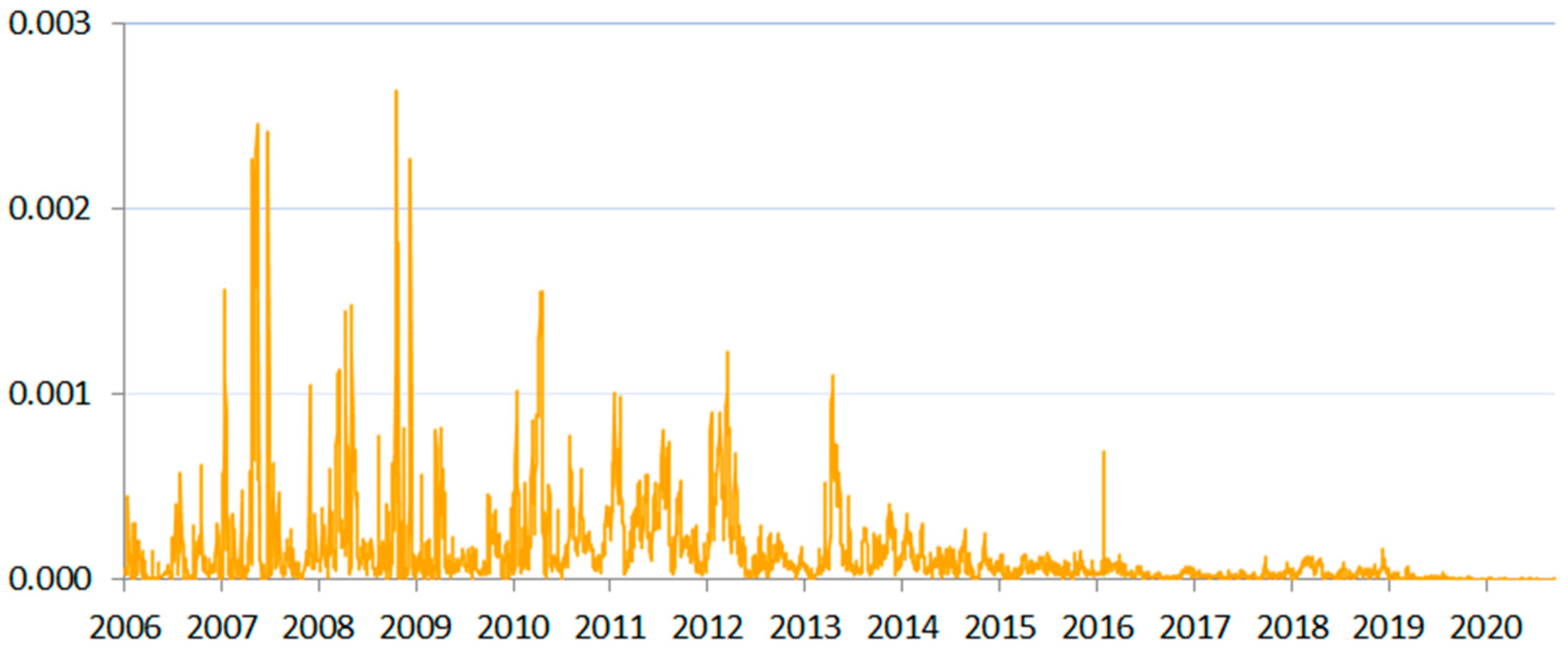
Figure 7.
SIN measure for Estonia between 2006 and 2020.
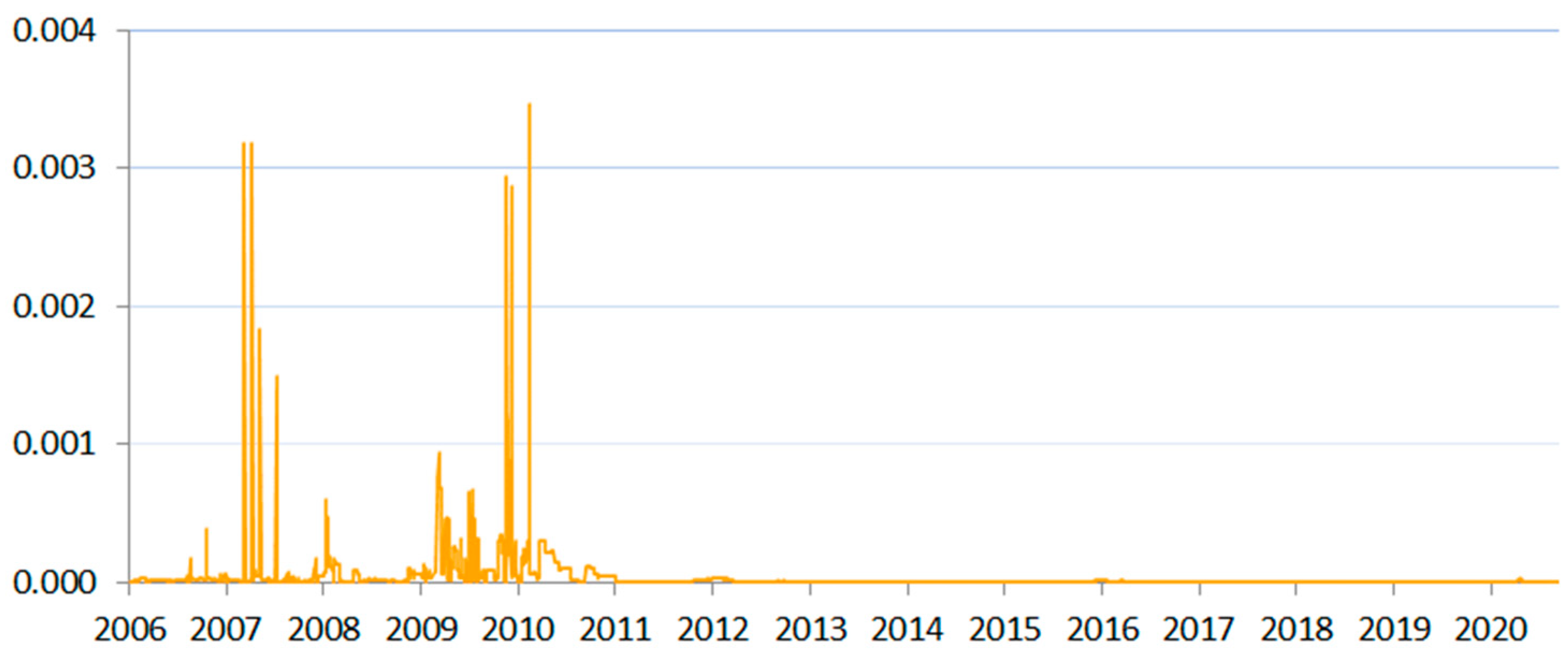
Figure 8.
SIN measure for Lithuania between 2006 and 2020.

Figure 9.
SIN measure for Latvia between 2006 and 2020.

Figure 10.
SIN measure for Slovakia between 2006 and 2020.
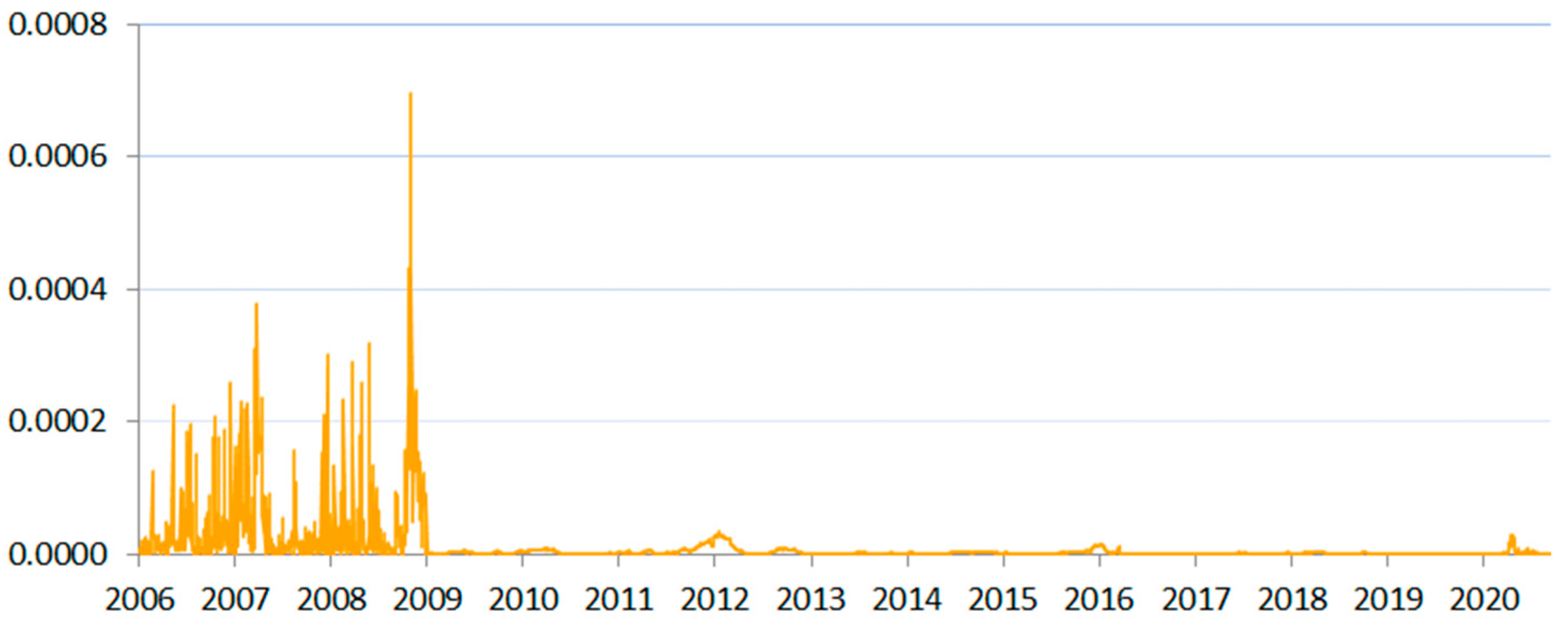
Figure 11.
SIN measure for Estonia, Latvia, Lithuania, and Slovakia (euro area) between 2019 and 2020. To compare the scale of risk with previous years, see Appendix A.
Figure 11.
SIN measure for Estonia, Latvia, Lithuania, and Slovakia (euro area) between 2019 and 2020. To compare the scale of risk with previous years, see Appendix A.

Table 1.
The studies of illiquidity effects categorized by the focus and sector of the financial system.
Table 1.
The studies of illiquidity effects categorized by the focus and sector of the financial system.
| Systemic Risk Occurrence | Liquidity Effects | Primary Sector of Occurrence | Other Sectors Possibly Affected by the Effect | Authors |
|---|---|---|---|---|
| Illiquidity exposure | Correlated exposures to illiquidity, free-riding | Banking sector | Shadow banking | Bhattacharya and Gale (1987) |
| Maturity rat-race and excessive short-term debt 1 | Brunnermeier and Oehmke (2013) | |||
| Illiquidity contagion | Fire sales and their effect on prices | Financial assets markets | Banking sector, shadow banking, investment funds, SIFIs | Shleifer and Vishny (1992) |
| Market incompleteness and effects of illiquidity on prices | Allen and Gale (1994, 2000a, 2000b) | |||
| Snowball effect, in which the loss spiral interacts with a margin spiral 1 | Brunnermeier and Pedersen (2009) | |||
| Market illiquidity contagion | Cespa and Foucault (2014) | |||
| Illiquidity-driven crises | Constraints to arbitrage adding to illiquidity | Financial assets markets | - | Shleifer and Vishny (1997) |
| Arbitrage affecting liquidity both ways | Gromb and Vayanos (2002) | |||
| Runs caused by mark-to-market accounting | Banking sector, shadow banking, investment funds, SIFIs | Cifuentes et al. (2005) | ||
| Bank runs triggering illiquidity, which triggers further bank runs | Banking sector | Diamond and Rajan (2005) | ||
| Leverage, illiquidity spirals, and financial frictions | Brunnermeier et al. (2013) | |||
| Brunnermeier and Sannikov (2014) | ||||
| Informationally driven market freezes | Interbank market fragility due to fear of adverse selection | Banking sector | - | Flannery (1996) |
| Lack of information about the counterparty risk causes the banks to stop lending to each other upon large shocks | Caballero and Simsek (2013) | |||
| Interbank market freezes caused by information asymmetry | Heider et al. (2015) | |||
| Information asymmetry as a source of repo markets collapse | Financial assets markets | Banking sector, financial markets, shadow banking, investment funds, | Acharya et al. (2011) | |
| Collateral value vs. its price | Gorton and Ordonez (2014) |
The table categorizes papers investigating liquidity risk effects that are relevant for systemic risk. The reported effects are grouped into four types of systemic risk triggers and arranged according to financial system sector or segment. 1 A loss spiral occurs when the losses on a few assets induce the market participants to reduce their positions in many other assets. Then these sales depress market prices, prompting further losses; a margin spiral occurs when market participants apply higher margin requirements because of the reduced market liquidity. Both effects reinforce each other, increasing the pressure to sell more assets (Brunnermeier and Pedersen 2009).
Table 2.
Liquidity risk indicators.
| Quantity-Based Indicators | Price-Based Indicators | |
|---|---|---|
| Monetary liquidity | Base money and broader monetary aggregates | Policy and money-market interest rates |
| Access to central bank liquidity facility (e.g., bidding volume) | ||
| Monetary conditions indices | ||
| Foreign exchange reserves | ||
| Funding liquidity | Bank liquidity ratios | Unsecured interbank lending (Libor–OIS spreads) |
| Secured interbank lending (repo rates) | ||
| Bank net cash flow estimates | Margins and haircuts on repo collateral | |
| FX swap basis | ||
| Maturity mismatch measures | Violation of arbitrage conditions (bond–CDS basis, covered interest rate parity) | |
| Commercial paper market volumes | Spreads between assets with similar credit characteristics | |
| Qualitative surveys of funding conditions | ||
| Market liquidity | Transaction volumes | Bid–ask spreads on selected global assets |
| Qualitative fund manager surveys |
The table presents existing liquidity risk indicator types categorized in relation to the type of liquidity and the numerical base of the indicator. Indicators are limited to those used in systemic risk analysis. Source: Jobst (2012, p. 13).
Table 3.
Analysis of systemic illiquidity measures for applicability to CEE.
| Measure | Authors | Is the Application Possible? (Data Limitations) | Is Contemporaneous Measurement Possible? (Issues of Lags and Frequency) | Does it Facilitate Systemic Risk Analysis? (Coverage/Proxying the Whole Financial System) |
|---|---|---|---|---|
| Liquidity factor | Pastor and Stambaugh (2003) | YES | YES | NO |
| A set of interpretable parameters | Getmansky et al. (2004) | NO | x | x |
| Broader hedge-fund-based systemic risk measures | Chan et al. (2006) | NO | x | x |
| A system of liquidity risk charges (LRCs) | Perotti and Suarez (2011) | YES | NO | x |
| Contrarian strategy liquidity measure (CSL) | Khandani and Lo (2011) | YES | YES | NO |
| Price-impact liquidity measure (PIL) | Khandani and Lo (2011) | YES | YES | NO |
| Systemic Liquidity Risk Index (SLRI) | Severo (2012) | NO | x | x |
| Daily liquidity noise measure | Hu et al. (2013) | NO | x | x |
| Liquidity Mismatch Index (LMI) | Brunnermeier et al. (2014) | YES | NO | x |
| Systemic risk-adjusted liquidity (SRL) model | Jobst (2014) | YES | NO | x |
| Systemicness | Greenwood et al. (2015) | NO | x | x |
| Cumulative Distance to Default (CDD) | Karkowska (2015) | YES | NO | x |
| Aggregate vulnerability (AV) and illiquidity concentration | Duarte and Eisenbach (2019) | NO | x | x |
The table presents the step-by-step process used to find a systemic liquidity risk measure by answering three questions (YES/NO). A negative answer to a given question eliminated the measure from further analysis (x).
Publisher’s Note: MDPI stays neutral with regard to jurisdictional claims in published maps and institutional affiliations. |
© 2021 by the authors. Licensee MDPI, Basel, Switzerland. This article is an open access article distributed under the terms and conditions of the Creative Commons Attribution (CC BY) license (https://creativecommons.org/licenses/by/4.0/).
Share and Cite
MDPI and ACS Style
Dziwok, E.; Karaś, M.A. Systemic Illiquidity Noise-Based Measure—A Solution for Systemic Liquidity Monitoring in Frontier and Emerging Markets. Risks 2021, 9, 124. https://0-doi-org.brum.beds.ac.uk/10.3390/risks9070124
AMA Style
Dziwok E, Karaś MA. Systemic Illiquidity Noise-Based Measure—A Solution for Systemic Liquidity Monitoring in Frontier and Emerging Markets. Risks. 2021; 9(7):124. https://0-doi-org.brum.beds.ac.uk/10.3390/risks9070124
Chicago/Turabian StyleDziwok, Ewa, and Marta A. Karaś. 2021. "Systemic Illiquidity Noise-Based Measure—A Solution for Systemic Liquidity Monitoring in Frontier and Emerging Markets" Risks 9, no. 7: 124. https://0-doi-org.brum.beds.ac.uk/10.3390/risks9070124
Note that from the first issue of 2016, this journal uses article numbers instead of page numbers. See further details here.