
One-Year and Ultimate Reserve Risk in Mack Chain Ladder Model


1
Institute of Econometrics, SGH Warsaw School of Economics, Niepodległości 162, 02-554 Warsaw, Poland
2
Risk Department, Sopockie Towarzystwo Ubezpieczeń ERGO Hestia SA, Hestii 1, 81-731 Sopot, Poland
*
Author to whom correspondence should be addressed.
Risks 2021, 9(9), 152; https://0-doi-org.brum.beds.ac.uk/10.3390/risks9090152
Submission received: 26 June 2021
/
Revised: 17 August 2021
/
Accepted: 18 August 2021
/
Published: 25 August 2021
(This article belongs to the Special Issue Quantitative Risk Measurement and Management)
Abstract
:We investigate the relation between one-year reserve risk and ultimate reserve risk in Mack Chain Ladder model in a simulation study. The first goal is to validate the so-called linear emergence pattern formula, which maps the ultimate loss to the one-year loss, in case when we measure the risks with Value-at-Risk. The second goal is to estimate the true emergence pattern of the ultimate loss, i.e., the conditional distribution of the one-year loss given the ultimate loss, from which we can properly derive a risk measure for the one-year horizon from the simulations of ultimate losses. Finally, our third goal is to test if classical actuarial distributions can be used for modelling of the outstanding loss from the ultimate and the one-year perspective. In our simulation study, we investigate several synthetic loss triangles with various duration of the claims development process, volatility, skewness, and distributional assumptions of the individual development factors. We quantify the reserve risks without and with the estimation error of the claims development factors.
1. Introduction
Insurance companies are exposed, among others, to reserve risk. The ultimate reserve risk is the risk that the current loss reserves will not be adequate in ultimate horizon, i.e., after the full run-off of liabilities. The one-year reserve risk is the risk that the current loss reserves will not be adequate after one year. The one-year view is an important notion introduced by Solvency II Directive, and it differs from the ultimate view which is traditionally analysed by actuaries. In the one-year view, we predict only the next year losses to be paid by the company and evaluate the loss reserve at the end of the next year for the further run-off of the liabilities, whereas, in the ultimate view, we predict all the future losses to be paid until all claims are settled.
One-year and ultimate reserve risks in Mack Chain Ladder model have been deeply studied in the literature; see, e.g., Mack (1993, 1994), Wüthrich and Merz (2008b, 2015), Röhr (2016), Gisler (2019) and England et al. (2019). In these papers, the authors focus on the reserve risk measured with the mean squared error of prediction and derive important relations between the prediction errors for the future losses to be covered in one-year and ultimate horizon. However, the relation between one-year and ultimate reserve risks has not been investigated for risk measures other than the mean square error of prediction, as closed formulas are no longer possible to achieve and additional distribution assumptions on the claims development process have to be imposed. For solvency purposes and economic models, we are more interested in measuring the reserve risk with Value-at-Risk, and, for this purpose, we have to use simulation methods with pre-specified distributions of the individual claims development factors. Hence, one-year and ultimate reserve risks are still worth studying in more detail.
Simulation methods which allow us to derive the distribution of the ultimate loss and measure the ultimate reserve risk are now well understood; see, e.g., England and Verrall (2002), Wüthrich and Merz (2008a) and Carrato et al. (2016). However, there is still a debate in the actuarial profession on what would be the most efficient way to derive the distribution of the one-year loss and measure the one-year reserve risk. The approach to modelling of one-year risk is discussed in the following works: Wacek (2007), White and Margetts (2010), Robbin (2012) and Papachristou (2016). The recent report of the Institute of Faculty of Actuaries by Scarth et al. (2020) lists and discusses three approaches to measuring the one-year reserve risk:
- The Merz-Wüthrich formula,
- The actuary-in-the-box, and
- Emergence patterns.
The Merz-Wüthrich formula plays a fundamental role in quantifying the one-year reserve risk. However, it cannot be applied if: (a) we measure the reserve risk with VaR, or any risk measure other than the mean square error of prediction without further assumptions, (b) we use an estimation method for the claims development factors other than the classical Chain Ladder estimators, e.g., we fit a smooth curve to the crude estimates or attach weights to individual claim development factors, and (c) we use an estimate of the reserve different from the Chain Ladder estimate. Similar arguments also apply to the Mack formula, which is derived under the same assumptions as the Merz-Wüthrich formula. A general approach to measure the one-year reserve risk was developed by Ohlsson and Lauzeningks (2009) and is based on the concept of the actuary-in-the-box, where we simulate the claims development in the next year (the next diagonal of the loss triangle) with the underlying model and then apply the same (as today) reserving algorithm at the end of the next year. This requires another estimation of the model with additional observations on the new diagonal of the loss triangle (the so-called re-reserving step). This process is much more time-consuming in simulations, compared to the ultimate reserve risk, due to the re-reserving step at the end of the next year. In addition, this process might be complex in implementation and is more vulnerable to unstable results since, a priori, we cannot describe all rules for the exclusion of extreme simulated individual claims development factors which should not be used for the re-estimation of the model, as well as we cannot fully capture the decisions which would be made by the reserving actuary in the real-world when new observations fill the diagonal of the loss triangle and the new estimate of the reserve is derived. If the actuary-in-the-box method may lead to implausible results, which are hard to validate, or is computationally too expensive, the third common approach in practice to quantifying the one-year reserve risk is an emergence pattern. The idea of the emergence pattern is to scale the ultimate reserve risk to the one-year risk. As pointed out in Dal Moro and Lo (2014), the scaling of the distribution of the ultimate loss to the one-year loss using simple ratios has become a practical way for insurance companies to adjust their economic models to Solvency II requirements. Some insurance companies may prefer, and to our knowledge they indeed prefer, to simulate the ultimate loss from a well-understood distribution which describes the reserve risk in ultimate horizon, allocate the simulated ultimate loss to a one-year loss and then estimate a risk measure in one-year horizon from this sample, instead of simulating the next year losses and re-calculating the loss reserve at the end of the next year. This approach may indeed be desirable since distributions of the ultimate loss and risk measures in ultimate horizon have been investigated by actuaries for many years before Solvency II, they reflect the traditional actuarial view of reserve risk and are used in planning reports and long-term risk analysis. However, in order to properly apply emergence patterns, we should know the true relation between the one-year reserve risk and the ultimate reserve risk for a claim development process in Mack Chain Ladder model, and this relation has not been investigated in the actuarial literature so far, except the case when the reserve risk is measured with the mean square error of prediction.
Bird and Cairns (2011); England et al. (2012) were the first who introduced concepts of an emergence pattern and emergence factors in reserve risk. England et al. (2012) suggest that the ultimate loss can be mapped to the one-year loss by using a simple linear function where one uses scaling ratios derived from the Merz-Wüthrich and the Mack prediction error. As a result, the conditional distribution of the one-year loss given that the ultimate loss is trivially, but incorrectly, defined (it is a degenerate distribution), and the simulation of a one-year loss from an ultimate loss, as well as the estimation of the one-year risk from a simulated sample of ultimate losses, is greatly simplified. To our knowledge, from actuarial practice, the linear emergence pattern formula is used by some insurance companies to model the one-year reserve risk (as well as the one-year premium risk), and Scarth et al. (2020) confirms that emergence patterns are vital in the actuarial practice. If the reserve risks are measured with the mean square error of prediction, then we can correctly switch from the ultimate risk/the ultimate loss to the one-year risk/the one-year loss by applying the linear emergence pattern formula, since the linear emergence pattern formula is constructed so that it fits the first two moments of the one-year and the ultimate loss. In this paper we are concerned about the relations between the distribution of the one-year loss, the distribution of the scaled ultimate loss derived from the linear emergence pattern and the distribution of the true emergence pattern of the ultimate loss in Mack Chain Ladder model. These questions about emergence patterns are raised for the first time in the actuarial literature.
We consider the classical Mack Chain Ladder model. In practice, we would not apply the linear emergence pattern formula in the classical Mack Chain Ladder, we would rather apply it in a version of the Mack Chain Ladder with more complex and time-consuming re-estimation algorithm with the new simulated data on the diagonal of the loss triangle and re-reserving algorithm. However, given that the analysis of the linear emergence pattern formula is missing in the actuarial literature, we start with the classical, and the simplest, Chain Ladder model.
The first goal of this paper is to validate if we can use the linear emergence pattern formula if the reserve risks are measured with Value-at-Risk. Our simulations show that the linear emergence pattern formula still works very good for loss triangles with short duration, low volatility, and skewness of individual development factors. However, the misestimation error of the one-year reserve risk (overestimation and underestimation) might be significant for loss triangles with long duration, large volatility, and skewness of individual development factors if we measure the one-year reserve risk with Value-at-Risk and use the linear emergence pattern formula to map the ultimate loss to the one-year loss. In general, the ultimate risk is scaled in a non-trivial (non-linear) way to the one-year risk. Hence, the linear emergence pattern formula should be applied with care, and, preferably, an improved version of the emergence pattern formula should be found.
The second goal of this paper is to improve the linear emergence pattern formula and estimate the true emergence pattern of the ultimate loss, i.e., the distribution of the one-year loss given the ultimate loss, from which we can properly derive a risk measure for the one-year horizon from a simulated sample of ultimate losses. We discuss how to estimate this distribution by fitting a mixture of gamma distributions with neural networks using the method recently developed by Delong et al. (2020). We demonstrate with an example that the true emergence pattern of the ultimate loss in a Chain Ladder model can be significantly different from the linear emergence pattern. To the best of our knowledge, this is the first attempt in the actuarial literature to derive the true emergence pattern of the ultimate loss in Mack Chain Ladder model. We also show that we can improve the calculation of the one-year risk measure from the simulations of the ultimate losses if we use our conditional distribution, instead of the linear emergence pattern formula.
The third goal is to test if classical actuarial distributions can be used for modelling of the outstanding loss from the ultimate and the one-year perspective in Mack Chain Ladder models. It is often believed among practitioners that the distributions of the outstanding loss in Mack Chain Ladder models can be approximated with a simple lognormal distribution, independently of the distribution of the individual development factors in the loss triangle (see, e.g., Mack 1994 and CEIOPS 2010). We consider different distributions of individual development factors. We conclude that the range of distributions: gamma, lognormal, and inverse gamma, which are recommended in Dal Moro and Krvavych (2017), based on authors’ practical experience, but not tested in any way, may not be sufficient to model the outstanding loss. Additionally, the choice of the best distribution depends on the characteristic of the underlying claims development model. Moreover, a simple enhancement of distribution made by fitting a shifted distribution may provide superior goodness-of-fit results.
In our simulation study, we investigate several synthetic loss triangles. The use of synthetic triangles, instead of real triangles, guarantees comparability of the results between the triangles investigated. We believe that the synthetic triangles created for this study reflect real triangles observed in actuarial practice. We start with the case where we quantify the reserve risks without the estimation error, i.e., we assume that all parameters of the claims development model are known. Such an approach requires less assumptions, which is beneficial given that we work with synthetic triangles. Our results on the one-year and ultimate reserve risks without the estimation error already shed light on emergence patterns. Next, we also present results for the reserve risks with the estimation error. The conclusions are similar in both cases.
We would like to remark that, in our first paper, as in Delong and Szatkowski (2020), we validate the adequacy of the linear emergence pattern formula in the context of premium risk and prove weaknesses of the linear emergence pattern formula by establishing analytical results in the following claims development models: Gaussian Incremental Loss Ratio model, Hertig’s model, Over-Dispersed Poisson model, and, in some abstract claims, development models. We point out that the results which we derived for premium risk also hold for reserve risk in the claims development models considered in Delong and Szatkowski (2020).
In Section 2, we introduce foundations of reserve risk modelling, including key definitions and formulas which we use in the paper. In Section 3, we provide the assumptions of our simulation study. The results of the simulation study are presented in Section 4. In Section 4.1, we validate the linear emergence pattern formula without the estimation error. In Section 4.2, we estimate the true emergence pattern of the ultimate loss in a Mack Chain Ladder model without the estimation error and demonstrate that it can differ from the linear emergence pattern formula. In Section 4.3, we include the estimation error and validate the linear emergence pattern formula. Finally, in Section 4.4, we test possible distributions of the outstanding loss from the ultimate and the one-year perspective with the estimation error.
2. Foundations of Reserve Risk Modelling
In this section, we introduce the so-called claims development result, one-year loss, ultimate loss, and outstanding loss, recall Mack Chain Ladder model, and present the linear emergence pattern formula from England et al. (2012) and Bird and Cairns (2011). We follow Mack (1993), Wüthrich and Merz (2008a, 2008b, 2015) and England et al. (2019), where we refer the reader for details. There is also an extensive literature on other aspects of applications of Chain Ladder method in claims reserving; see, e.g., Reference Buchwalder et al. (2006), Merz and Wüthrich (2015) and Harnau (2018), Peremans et al. (2018).
2.1. Claims Development Result and Reserve Risk
Let denote the accident year and denote the development year initiated with respect to the accident year. We consider a sequence of random variables , where denotes the cumulative payments made for the i-th accident year up to the j-th development year. We assume that all claims are settled within n years since their occurrence. Consequently, the variable denotes the ultimate loss for the i-th accident year, and denotes the ultimate loss for the loss triangle.
We study a discrete stochastic model with time steps , where k denotes a calendar year. We introduce the filtration:
which describes the information available at the end of the k-th calendar year. For a given calendar year , we introduce the outstanding loss at the end of the k-th calendar year, respectively, from the ultimate perspective and the one-year perspective:
for with if and if , the best estimate of the ultimate loss at the end of the k-th calendar year:
and the claims development result for reserve risk from the perspective of the end of the k-th calendar year, respectively, in one-year horizon and ultimate horizon:
and
The claims development result with negative sign represents the loss to which the company is exposed (in the terms of basic own funds, in line with Solvency II requirements). Hence, the claims development results for reserve risk (1) and (2) with negative sign are called, respectively, the one-year loss and the ultimate loss for reserve risk. We remark that is similarly called the ultimate loss, but there should be no confusion in the sequel. Given the calendar year and the available information , the random variables and are used to model the ultimate reserve risk, while and are used to model the one-year reserve risk. The value is -measurable; hence, it is deterministic at time step k.
From now on, we assume that we are at time step , the information is available, and we quantify the reserve risk at the end of the n-th calendar year.
2.2. Mack Chain Ladder Model
The claims development process in Mack Chain Ladder model satisfies the following three assumptions:
- CL1:
- The cumulative payments of different accident years are independent,
- CL2:
- There exist parameters such that
- CL3:
- There exist parameters such that
In addition, in our simulation study, we assume that:
- CL4:
- The cumulative payments are a Markov process for each accident year .
The last assumption allows us to use parametric conditional distributions of , fitted to the first two moments, for claims development. In the sequel, we will also use the so-called individual claims development factors . It is straightforward to set the assumptions CL1:CL4 for .
Given , the above assumptions imply that:
The formulas can be substituted into the claims development results (1) and (2). Once we specify the distributions of , and their parameters and , we can measure the risk of the one-year loss and the ultimate loss, given , by simulating for and performing the calculations (1)–(3). This approach is sufficient if we do not allow for the estimation error in the reserve risk. It is a standard practice in claims reserving to include the estimation error of the parameters in the reserve risk, as this estimation error can be quantified with a closed formula with the mean square error of prediction in one-year and ultimate horizon.1 In a simulation model, the estimation error is taken into account by sampling new values of the claims development factors from the distribution of the estimators, simulate the future claims development with the distributions of with the parameters and and, for the one-year risk, re-reserve by re-estimating the best estimate of the ultimate loss with another estimates of using the simulated observations on the diagonal of the loss triangle.
In the sequel, we use Equations (1.1), (1.2), (2.2), (2.3) from Wüthrich and Merz (2015), which give the analytical formulas the mean square error of prediction for
where, in all cases, we use 0 as the predictor. These formulas are also discussed in Röhr (2016) and Gisler (2019). In a simulation model, the mean square error of prediction is replaced with variance of the simulated claims development result.
2.3. The Linear Emergence Pattern Formula
England et al. (2012) and Bird and Cairns (2011) postulated a linear relation between the best estimate of the ultimate loss and the ultimate loss, which we call the linear emergence pattern formula. In our paper, we follow the first method from England et al. (2012), which is based on ultimate losses, not on reserves, using two different approaches.
The first approach is based on the emergence pattern of the ultimate loss for an accident year, given , which is described with the equation:
with the emergence pattern factors :
We point out that, in contrast to from (3) which is -measurable, the random variable from (4), which we use to approximate , is now -measurable. If we aggregate over all accident years, we get the linear emergence pattern of the ultimate loss based on individual accident years, given :
If we allow for the estimation error, then ≠, even though = for each accident year i, since the estimation error introduces correlations between the simulated ultimate losses in accident years, which are different from the one-year and ultimate perspective. To account for this correlation, the emergence factors have to be scaled to guarantee that . There is no universal method in actuarial practice how this scaling should be done.
The second approach is based on the use of the linear emergence pattern of the ultimate loss directly based on all accident years combined, given :
where the single emergence pattern factor is defined by
This time, the single emergence pattern factor reflects the correlations between the ultimate losses in accident years simulated with the estimation error.
The idea of the emergence pattern formula is that, instead of simulating the individual development factors for the next year development in the loss triangle and projecting the best estimate of the ultimate loss at the end of the next year, we simulate the ultimate loss or and allocate it to the best estimate of the ultimate loss at the end of the next year with or . For this approach, the distribution of the ultimate loss has to be specified. In practice, this distribution is derived by simulating the full run-off of the loss triangle with the pre-assumed claims development process, possibly taking into account the parameters’ uncertainties. Once the ultimate losses are simulated, they are linearly scaled and the one-year reserve risk can be estimated from the simulated sample.
The main question is to which extent the distributions of , , may differ in practice, where, by the distributions, we mean the conditional distributions of the objects given the information available in a loss triangle. We are also interested in how the distributions of are related to the distribution of . We compare the distributions by estimating the Value-at-Risk measures in simulations. If we apply the linear emergence pattern formula for all accident years combined (6), then we have the following scaling rule for the VaR risk measure:
for all confidence levels , which implies that the ultimate reserve risk, measured with VaR, should be scaled with a simple coefficient to get the one-year risk. In particular, we validate if this simple scaling rule can be applied in practice.
The reason why the distributions of , , and are expected to be different is that the linear emergence pattern Formulas (5) and (6) are unlikely to give the proper relation between the best estimate of the ultimate loss and the ultimate loss. By the definition of the emergence factors, the linear emergence pattern formulas only give proper relation for the first two moments of the distributions in which we are interested. Given the multivariate distribution of the claims development process, which we assume to be specified with its parameters, we could try to derive the conditional distributions for accident years . This approach would improve the linear emergence pattern formula, without the estimation error, and we would reveal the true emergence pattern of the ultimate loss in Mack Chain Ladder models. Since a closed form solution is not possible, we estimate the conditional distributions from simulated losses. We use and to denote our key objects for accident year i derived from and the estimated conditional distribution of . A similar approach is possible with the estimation error, but we would have to estimate the conditional distributions for accident years , which would be hard to compare with the linear emergence pattern formula. We leave this for further research.
3. The Assumptions of the Simulation Study
We construct four loss triangles for our study, which we call low, medium, high, and very high, depending on duration of the claims development process, volatility, and skewness of individual development factors.
First, we start with defining the loss triangles for the study of the reserve risk without the estimation error. When setting historical loss triangles, i.e., the realizations in , we do the following:
- We fix the payments in the first development year for all accident years and project the future cumulative payments on the expected value basis. This means that the last diagonal of a loss triangle is equal to . Such a construction of loss triangles makes it easier to compare our results with respect to different distributions of since the results are not influenced by random differences in the last diagonal in the constructed loss triangles. We would like to point out that, in the case without the estimation error, the diagonal of the loss triangle is the only element of the historical loss triangle used in the study due to the Markov nature of the claims development process and no need to re-estimate the parameters with historical observations.
In order to come up with particular values for and , which describe the claims development process, we make the following (reasonable) assumption:
- A loss triangle with a longer duration and a longer tail has a higher volatility and skewness of the outstanding loss measured with coefficient of variation and skewness coefficient, which is presented in Dal Moro and Krvavych (2017).
This might not always be the case in practice since we also observe loss triangles with high duration and low volatility, skewness. However, as we will observe in the sequel, the assumption made above allows us to create loss triangles more interesting from the point of our study. While setting different parameters, we generally consider the parameters for paid triangles; however, the presented methodology can be also extended for incurred triangles.
- Development factors : We follow the approach from Guy Carpenter and Oliver Wyman (2014) to describe the pattern of loss development. We use a duration of the claims development process, and we calculate a version of the Macaulay duration:where denote the incremental payments made in development year j for accident year i. The duration (8) in Mack Chain Ladder model is independent of the accident year. Based on Guy Carpenter and Oliver Wyman (2014) and England et al. (2012), durations of claims development processes usually range from 1 to 6 years. A line of business with the duration higher than 3 is interpreted in this paper as long-tailed.
We construct development factors for our four loss triangles by specifying and matching durations. We model with exponential or power curves, which is the standard approach; see, e.g., Institute of Actuaries (2002). We prefer power curves for long-tailed lines of business, as they allow for slower convergence to 1. As exponential and power curves require two parameters, we specify as the second reference point, next to the duration of the claims development process, which we use for fitting . We choose based on KNF (2020) and Guy Carpenter and Oliver Wyman (2014), and we follow the assumption that a longer and more volatile claims development process generally tends to have a higher . Again, this might not always be the case since we observe loss triangles with low and high duration in Guy Carpenter and Oliver Wyman (2014); KNF (2020). The benefits of this assumption are that it allows us to fit a smoother curve to given duration and and leads to more interesting conclusions.
The maximal development year for a loss triangle, denoted by n, is chosen in line with the rule of thumb presented in Carrato et al. (2016), and we guarantee that , where d denotes the duration.
We set the parameters:
- Low: , , and . Curve type-exponential.
- Medium: , , and . Curve type-exponential.
- High: , , and . Curve type-power.
- Very high: , , and . Curve type-power.
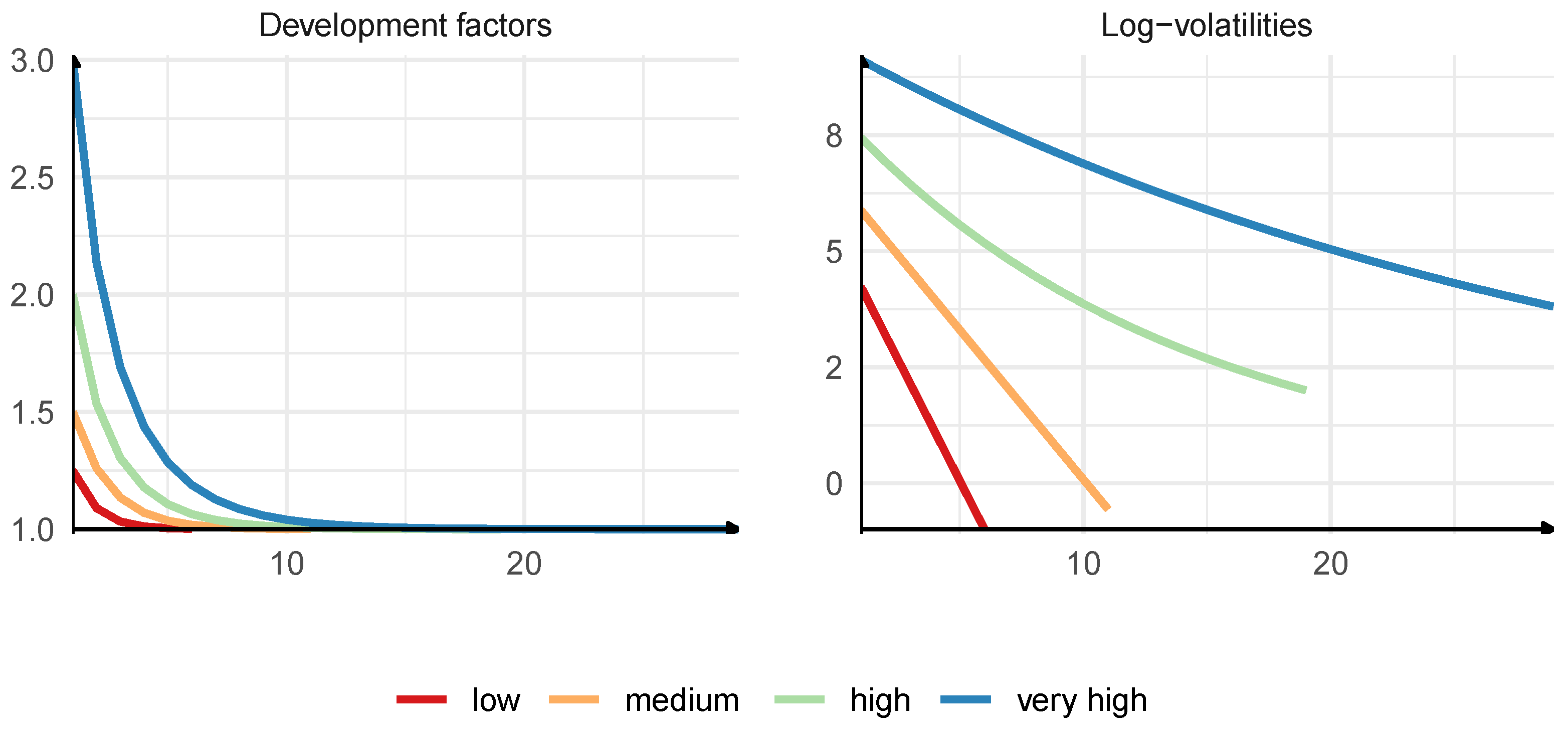
We use numerical optimization to fit curves to given duration of the claims development process and initial value . The development factors for four loss triangles are presented in Figure A1.
- Volatilities : We follow the approach from Dal Moro and Krvavych (2017) to describe the volatility of loss development. We use the coefficient of variation (CoV) and the skewness-to-CoV ratio (SC) of the outstanding loss from the ultimate perspective.
We again construct volatilities with power curves. This time, we only use power curves because we require that the volatilities converge slower to 0 than the claims development factors converge to 1, which we observe in KNF (2020); see Figure A2. We fit power curves to pre-specified CoV and SC ratios of the outstanding loss. We have found the following references about potential values of CoV and SC:
- Dal Moro and Krvavych (2017) state that reserve risk profiles should have CoV in the range from 6% to 70%, with reserve risk profiles assessed as most risky for CoV exceeding 25%. For SC ratios, their range starts at 1.9, and the ratios above 4 describe most risky reserve risk profiles.
- Wüthrich and Merz (2008b) investigate CoV for different portfolios and observe the values from 1.9% to 51.7%, with most values in the interval from 3.5% to 16.5%.
- In the Standard Formula for reserve risk, as in Solvency II Regulation (2015), the lowest CoV is set to 5.5%, and the highest CoV is set to 22%. These values are used for one-year reserve risk; hence, CoV for ultimate reserve risk should be higher.
We set the following targets for coefficients of variation and skewness-to-CoV ratios of the outstanding loss from the ultimate perspective (without the estimation error):
- Low: and . Curve type-power.
- Medium: and . Curve type-power.
- High: and . Curve type-power.
- Very high: and . Curve type-power.
We include to allow for light-tailed claims development processes which we observe in KNF (2020). The value of is chosen since it is in the middle of the range of SC ratios in the reserve class, where Dal Moro and Krvavych (2017) suggests to use lognormal distributions to model the outstanding loss; see the next point, as well.
By the proof to Theorem 1 and Theorem 3 in Mack (1993), we calculate the first two moments of the outstanding loss from the ultimate perspective:
which we use to calculate the coefficient of variation, which we next use as the reference point in our fitting procedure. The calculation of the skewness coefficient of the outstanding loss is more problematic as it depends on higher moments and distributional assumptions of the claims development process, which are not specified in the distribution-free Mack Chain Ladder model. In Appendix A.1, we calculate the skewness of assuming that follow lognormal distributions, and we use this particular formula of the skewness coefficient to fit , even though in our numerical studies we also use different distributions of the individual development factors. The reason for that approach is that we want to have a curve for a loss triangle independent of the distribution of the individual development factors in the triangle so that we can investigate the impact of different distributions.
We use numerical optimization to fit curves to given coefficient of variation and skewness-to-CoV ratio of the outstanding loss. The volatilities for four loss triangles are presented in Figure A1.
- Distributions of For each loss triangle defined above, we run simulations with the distributions recommended by Dal Moro and Krvavych (2017):
- gamma.
- lognormal.
- inverse gamma.
Lognormal distribution is most commonly used in claims reserving, as in, e.g., England and Verrall (2002); Rehman and Klugman (2010), and it was also used in the calibration of the Standard Formula, as in CEIOPS (2010). In order to model light-tailed reserve risk profiles, gamma distribution could be considered, as in England and Verrall (2002), while, for heavy-tailed reserve risk profiles, we could implement inverse gamma distribution. Dal Moro and Krvavych (2017) also point out inverse Gaussian distribution; however, in our study, it gave very close results to lognormal distribution and was, therefore, discarded. Let us remark that, in our paper, we use the above distributions in a different context than Dal Moro and Krvavych (2017). We use these distributions as the distributions of the individual development factors , given , whereas Dal Moro and Krvavych (2017) use these distributions as the distributions of the outstanding loss given . In Section 4.4, we also check if the above distributions can be fitted to the outstanding loss in Mack Chain Ladder models. To the best of our knowledge, gamma and lognormal distributions are commonly used in practice for modelling individual development factors in Mack Chain Ladder models, as also seen in an example in Appendix 1 in England et al. (2019), and we include inverse gamma distribution to model heavy-tailed loss developments.
After the loss triangles and the parameters of the claims development processes were specified, we performed some plausibility checks to make sure that our triangles possess characteristics that we would expect them to have. The plausibility tests are presented in Figure A3 and they confirm that we have constructed reasonable historical loss triangles with reasonable stochastic loss developments. Of course, our triangles do not completely fill the space of possible loss triangles, but we believe that they represent crucial (and various) characteristics of claims development processes which actuaries face in practice. The very high triangles seem to be the most extreme case we may observe in real world, while other triangles seem to be commonly investigated by reserving actuaries.
Now, we move to the study of the reserve risk with the estimation error. The inclusion of the estimation error in our study requires additional assumptions for the construction of the historical loss triangles. From the formula for the mean square error of prediction for the one-year reserve risk from (1.2) for a single accident year and (2.3) for aggregated accident years in Wüthrich and Merz (2015), we can deduce that the reserve risk with the estimation error depends, not only on the diagonal of the loss triangle and the estimated model’s parameters,3 but also on the proportions of the cumulative historical payments made in development period j in the most recent calendar year to the cumulative historical payments made in that development period in all past calendar years, i.e., on , where here denotes a factor from Wüthrich and Merz (2015), not the emergence factor. Using KNF (2020), we can confirm that these proportions of the aggregate payments observed in our synthetic triangles, constructed above, are of reasonable magnitude and match real loss triangles from the Polish market. The next difficulty is that, when we sample the new value of the claims development factor for the introduction of the estimation error, by conditionally sampling in , the result depends, in general, on the values of the individual historical payments in each accident year . Fortunately, we did not observe qualitatively different results compared to the case where we use the synthetic loss triangles with the historical cumulative payments projected on the expected value basis. Naturally, there are numerical differences in the results; however, we are concerned with the nature and the shape of the relation between the one-year and the ultimate reserve risk, which do not differ qualitatively. For these reasons, in the study of the reserve risk with the estimation error, we use the same synthetic loss triangles, as described above, with the same claims development factors and volatilities. The difference is that now we sample the new estimates of the claims development factors, simulate the development of claims with the pre-specified distributions under these new parameters, re-estimate the claim development factors with the new payments on the diagonal of the loss triangle and derive the new reserve at the end of the calendar year with these new estimates. Finally, we have to scale the emergence factors for accident years if we allow for the estimation error; see Section 2.3. There are various scaling methods used in practice, as seen in Section 10.7 in Scarth et al. (2020), and the results depend on the methods. We use the simplest uniform scaling method based on .
Since we target CoV and SC of the outstanding loss from the ultimate perspective in a model with lognormal distribution of individual claims development factors and without the estimation error when we define the curves for , in Table 1, we summarise the final CoV and the SC of the outstanding loss from the ultimate perspective for the four triangles, the three distributions, and two cases: without and with the estimation error. The measures confirm that we have constructed reasonable simulation schemes for claims development processes which agree with Dal Moro and Krvavych (2017). The CoVs are calculated analytically and are presented for all distributions of together, as they are defined by the construction of triangle. The SCs without estimation error are calculated analytically following the equations in Appendix A.1, and, for the case with estimation error, they are calculated based on simulations. We do not present the values of SC for inverse gamma distribution, as it does not exist in this situation (as presented in Appendix A.1).
At the end, let us mention that payments are not discounted in simulations and the best estimates of ultimate losses are presented in nominal values.
4. The Results of the Simulation Study
First, we examine the true relation between the one-year reserve risk and the ultimate reserve risk, measured with Value-at-Risk, and validate the linear emergence pattern formula used for scaling ultimate losses to one-year losses in a model without the estimation error. Secondly, we discuss how one can extract the true emergence pattern of the ultimate loss in Chain Ladder models and demonstrate how to improve the linear emergence pattern formula if we would like to measure the one-year risk from a simulated sample of ultimate losses. We still investigate the case without the estimation error for the true emergence pattern in a Mack Chain Ladder model as it allows for a simpler comparison with the linear emergence pattern formula. Next, we validate the linear emergence pattern formula in a model with the estimation error. Finally, we study distribution approximations of the outstanding loss in ultimate and one-year time horizon with the estimation error and verify the fit of classical actuarial distributions.
4.1. One-Year vs. Ultimate Reserve Risk without the Estimation Error
For each triangle, we run simulations from the assumed claims development model by simulating the individual development factors and developing the loss triangle to the full square. We are interested in the ratios:
The first ratio (10) gives the true relation between the one-year risk and the ultimate risk. The second and the third ratios (11) and (12) give the relations between the one-year risk and the ultimate risk in case when the one-year loss is derived from the ultimate loss with the linear emergence pattern Formulas (5) and (6). From (7), we know that the ratio (12) for VaR is equal to the single emergence pattern factor independently of the distribution of the individual development factors. All risk measures are estimated based on simulations.
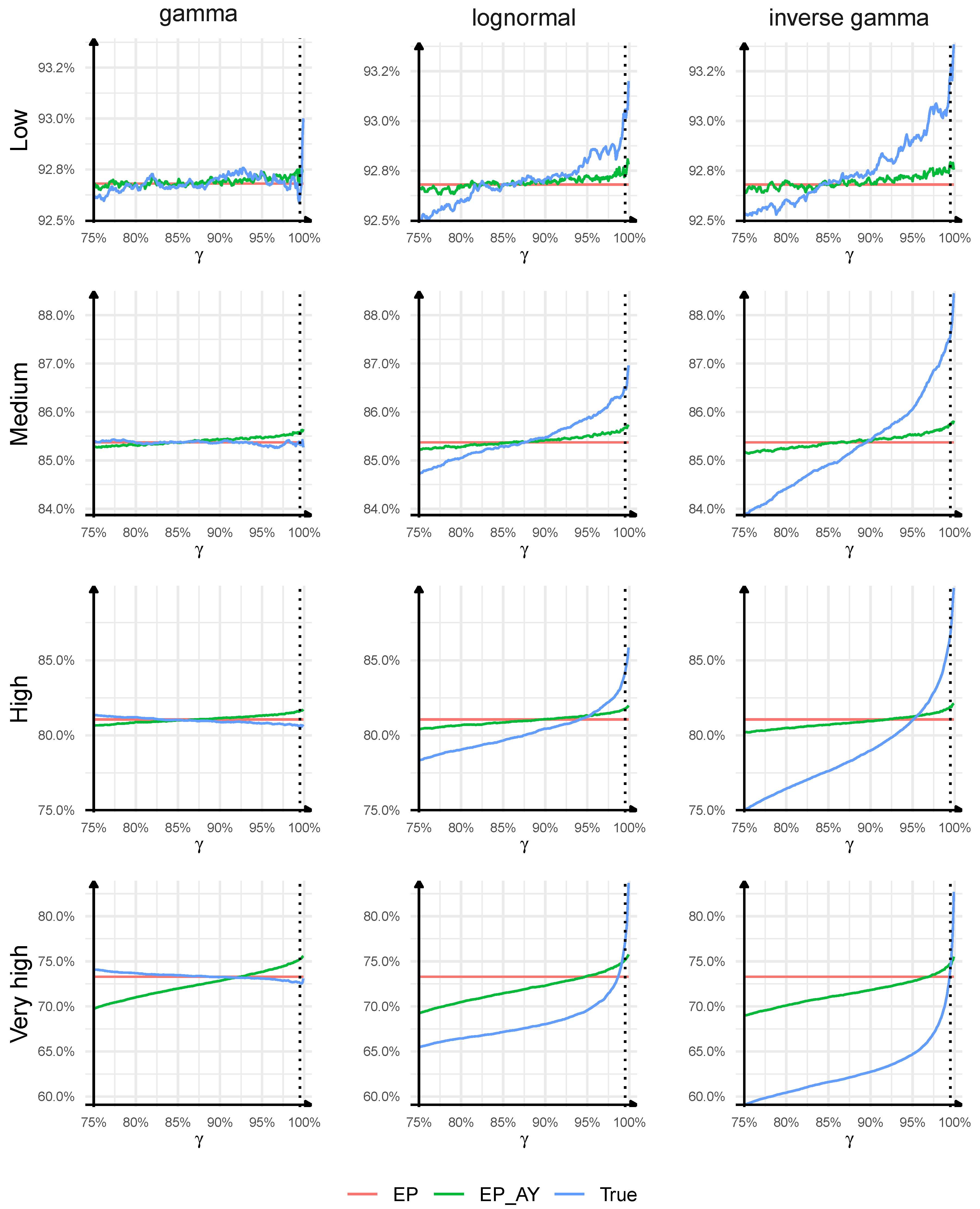
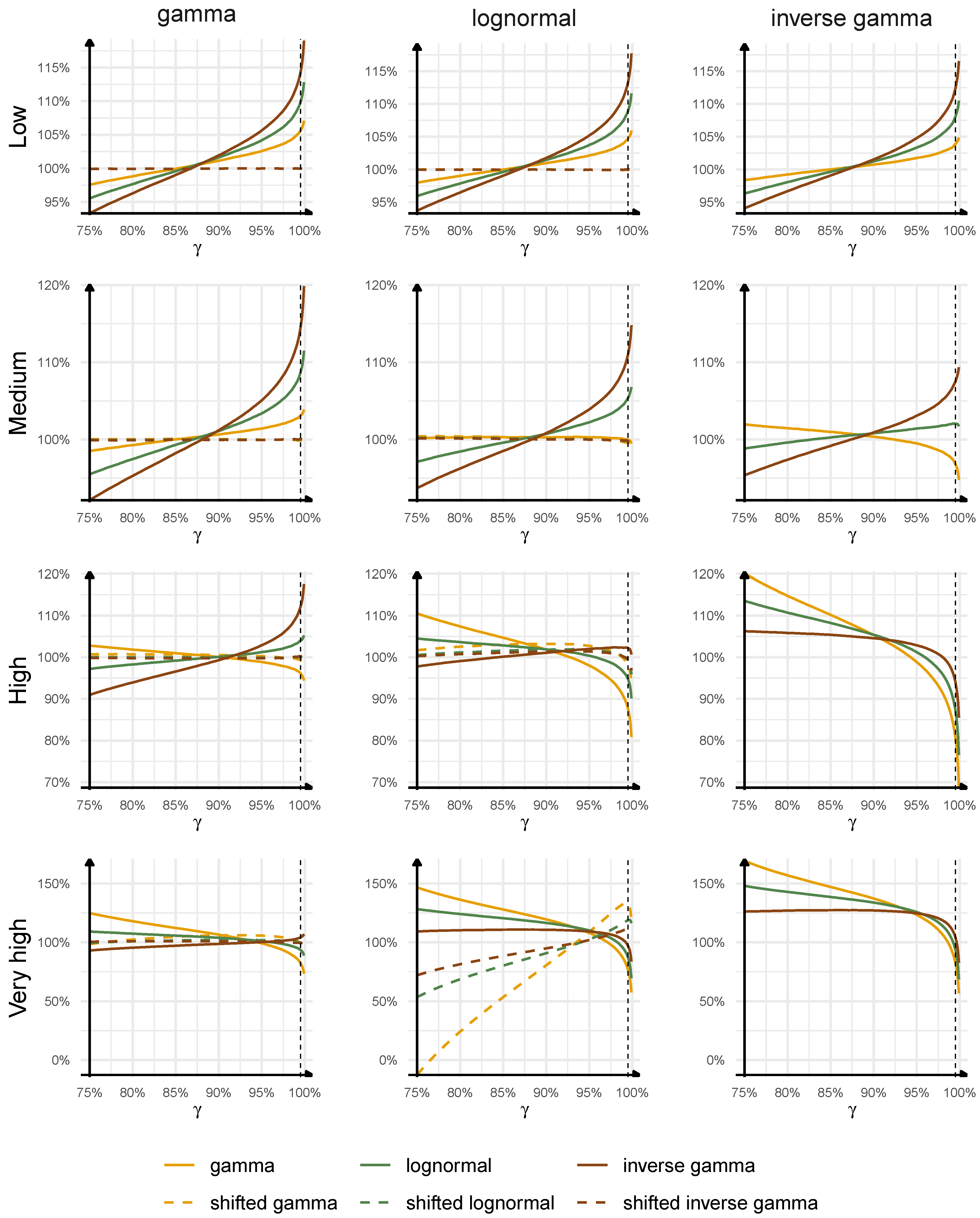
The results are presented in Figure 1. Each row represents a different triangle type, while each column represents a different distribution of the individual development factors in the loss triangle. The ratios (10) and (12) as a function of the confidence level are plotted, respectively, with blue, green, and red lines. We consider confidence levels from to , which are used in actuarial practice. The dashed vertical line in Figure 1 presents implied by Solvency II Directive.
First, we study the true relation between the one-year reserve risk and the ultimate reserve risk described by the ratio (10). We may notice that the ratios can be significantly different and, in general, depend on the confidence level, the distribution of the individual development factors in the loss triangle and the triangle type (the key characteristics of the claims development process). Interestingly, for lognormal and inverse gamma distributions, the ratio (10) seems to be an increasing function of the confidence level, whereas, for gamma distribution, it is a decreasing function of the confidence level. This property seems to hold universally for light-tailed and sub-exponential/heavy-tailed distributions of individual development factors (however, additional tests should be performed to confirm this statement; we also tested Weibull, Pareto, normal distributions in addition to the distributions presented in the paper). For low triangles, the true ratio of the one-year risk to the ultimate risk depends weakly on the confidence level and the distribution of the individual development factors. This is a very useful property of the one-year risk vs. the ultimate risk. As we move to triangles with longer duration, higher volatility, skewness, and heavier tail of individual development factors, the range of possible values of (10) for our confidence levels extends to – for high triangles with lognormal distribution, to – for very high triangles with lognormal distribution, and even to – for the most extreme case of very high triangle with inverse gamma distribution. For the triangles with gamma distribution, we observe similar values of (10) for all four triangles, with the widest range observed for very high triangle and being 72.6–74.2%. These examples show that the distribution of the individual development factors in the loss triangle and the key characteristics of the claims development process (such as duration, development pattern and its volatilities) should have an important impact on the relation between the one-year reserve risk and the ultimate reserve risk, and simple rules for scaling the ultimate risk to the one-year risk may misestimate the true risk. For example, for high triangles, for , we have the following ratios: , , , respectively, for gamma, lognormal, and inverse gamma, for we have the following ratios: , , , again for gamma, lognormal, and inverse gamma, whereas, for low triangles, the ratios are close to for all distributions and all confidence levels.
Secondly, we compare the two approaches to the linear emergence pattern Formula (5) with (6) by comparing the ratio (11) with (12). For all triangles, except very high, the ratios are very close to each other for all confidence levels considered. For very high triangles, the difference resulting from the two approaches is larger, e.g., for , the largest difference between (11) and (12) is observed for gamma distribution and the ratios are equal to for EP and for EP_AY, whereas, for , the largest difference is observed for inverse gamma distribution and the ratios are equal to for EP and for EP_AY. We can conclude that the linear emergence pattern formula applied to individual accident years does not lead to significantly different results from the linear emergence pattern formula applied to all accident years combined unless we work with triangles with very long duration, very high volatility, skewness, and heavy tails of individual development factors. We will continue with (5), which is more common in practice.
Thirdly, and most importantly, we analyse the adequacy of the linear emergence pattern Formula (5) in Chain Ladder models and its ability to estimate the one-year risk from ultimate losses. Already, from the first point of our analysis, we expect that the linear emergence pattern formula may give poor results in some important cases. We can deduce that, for low triangles, the quality of the linear emergence pattern formula is indeed very good, for all distributions and all confidence levels, and the maximal misestimation error of the one-year risk is equal to of the true one-year risk. The linear emergence pattern formula is worse for medium triangles with gamma or lognormal distributions, where the maximal misestimation error of the one-year risk is of the true one-year risk, and for medium triangles with for inverse gamma, where the misestimation error reaches . When we move to triangles with longer duration, higher volatility, skewness, and heavier tail of individual development factors, the performance of the linear emergence pattern formula deteriorates further and the misestimation errors depend on the triangle type, the distribution of the individual development factors in the loss triangle and the confidence level. For high triangles, for , the misestimation errors of the one-year risk are , , of the true one-year risk, respectively, for gamma, lognormal, and inverse gamma, while, for , the misestimation errors are , , , again for gamma, lognormal, and inverse gamma. For very high triangles, for all confidence levels considered, the maximal absolute misestimation error reaches , , for gamma, lognormal, and inverse gamma distributions. Interestingly, we can observe that, for lognormal distribution and inverse gamma, the linear emergence pattern formula overestimates the Value-at-Risk measure for low confidence levels and underestimates VaR for high confidence levels. A reverse behaviour is observed for gamma distribution where the emergence pattern formula underestimates the Value-at-Risk measure for low confidence levels and overestimates VaR for high confidence levels. This property seems to be universal for light-tailed and subexponential/heavy-tailed distributions of individual development factors, but as above, additional tests should be performed. We may conclude that the linear emergence pattern Formula (5) may lead to a significant misestimation of the one-year risk in case of volatile, skewed, heavy-tailed claims development processes with long durations. However, it may offer a reasonable approximation of the one-year risk in case of claims development processes with short durations, low volatilities, low skewness coefficients, and light tails.
4.2. The True Emergence Pattern of the Ultimate Loss without the Estimation Error
We choose the high triangle with the maximal development period set to and lognormal distribution of the individual development factors. This triangle is the most interesting for our analysis since the linear emergence pattern formula fails to estimate the true quantiles of the one-year loss and the claims development process for this triangle is still relevant for actuarial practice (we exclude very high triangles and inverse gamma distributions as they are less likely to arise in applications).
We simulate 10,000 scenarios of the revaluations of the best estimate of the ultimate loss in consecutive development years from the claims development model specified for the high triangle for a single accident year. Clearly, gives the ultimate loss . The subscript i is omitted as we do not consider any specific accident year in these simulations. First, we simulate the payments for the first development year, next we simulate the development process of claims in consecutive development years using the assumptions CL2–CL3 and lognormal distribution for the individual development factors, and finally we calculate the best estimate of the ultimate loss in each simulation at the end of each development year using the known development factors . The payments for the first development year are simulated from a uniform distribution on , where and denote the payments assumed for the high triangle in the first development year in the first and the last accident year. The scenarios are collected in the matrix of dimension 180,000 × 4. The range of the scenarios in should include, by construction, the range of possible scenarios of stochastic developments of claims from our loss triangle, which we derive if we simulate the future cumulative payments starting from the cumulative payments observed at the last diagonal of the loss triangle. In order to guarantee that we fit the model on the range of scenarios of claims development relevant for our high triangle, we additionally simulate 1000 scenarios of claims development and the revaluations of the best estimate of the ultimate loss for each accident year for the high triangle given the history . These scenarios are added to , and we end up with the matrix of dimension 198,000 × 4. Finally, the best estimates in are scaled with the mean value of the ultimate loss.
We train the so-called Gamma Mixture Density Networks and fit the conditional distributions of to the data in . The idea is to fit a mixture of gamma distributions to a noisy response where the mixing probabilities, the shape parameters, and the common scale parameter depend on explanatory variables; for details, we refer to Delong et al. (2020). In the data matrix , the response is , and the explanatory variables are given by . We apply the logarithmic and the min max scaler transform to and feed the inputs into the neural network.
We fit deep neural networks with 3 hidden layers, and we apply the forward network algorithm from Delong et al. (2020). The development period is treated as a categorical variable, and we use the entity embedding approach to model this variable. We test various hyper-parameters: the number of gamma densities = 3, 1, 2, 4, 5; the number of neurons in each layer = 20, 10, 30, 40; the learning rate = 0.0005, 0.0002, 0.002, 0.02; the dimension of the embedding = 5, 1, 2, 3, 4, 6; the batch size = 10,000 and 1000, and the first number is the optimal choice identified in our pre-training trials. A high dimension of the entity embedding is caused by the fact that the conditional distributions are significantly different at different development years k: they are skewed at initial development years and symmetric at later development years. The Expectation-Maximization algorithm is run for 500 iterations and the neural network is trained for 25 epochs in each iteration. The data set is split into training and validation in the proportion , and early stopping is applied on the validation set in each iteration of the EM algorithm.
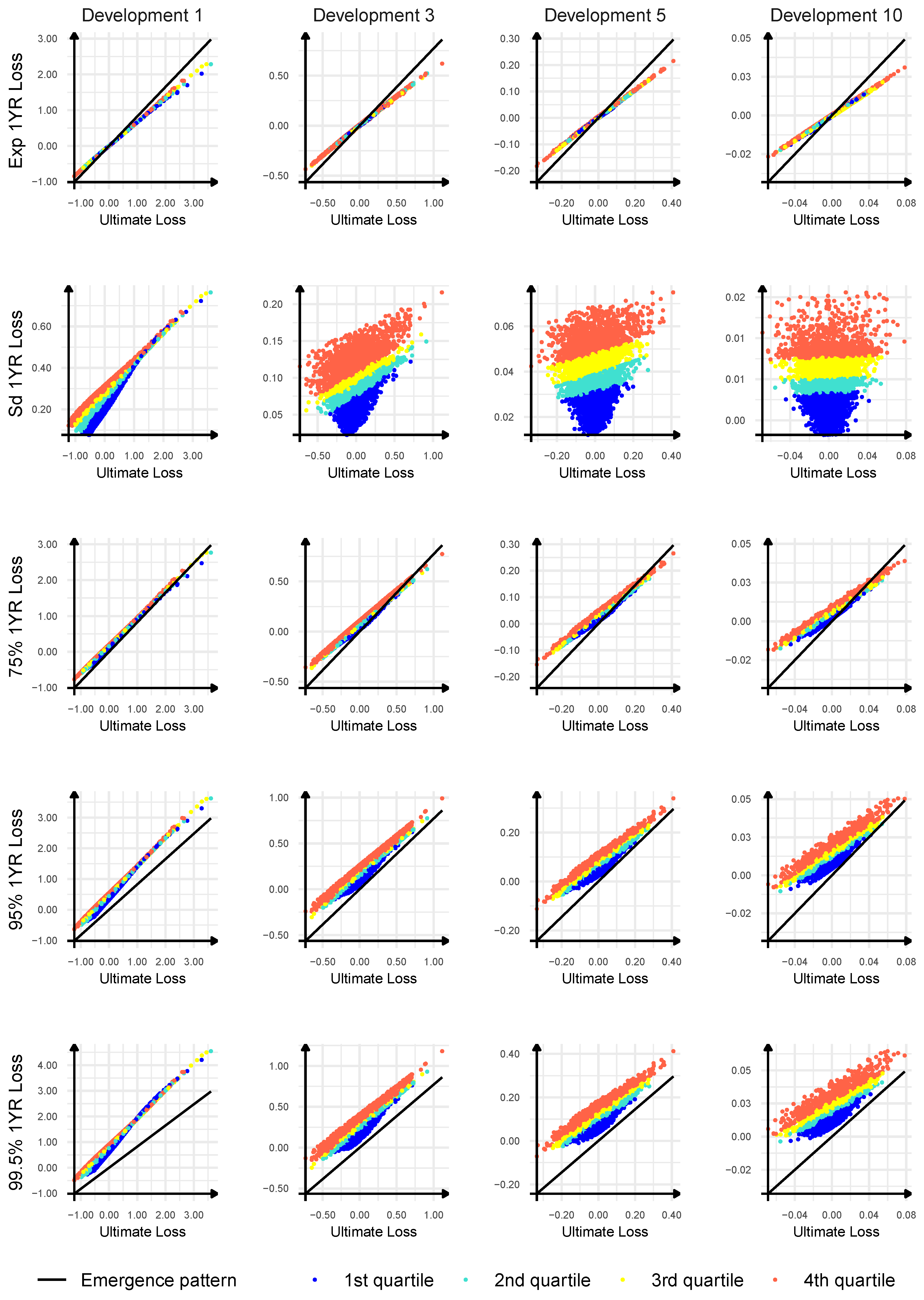
In Figure 2, we present key characteristics of the true emergence pattern of the ultimate loss, derived from the estimated conditional distributions of for , in a comparison with the linear emergence pattern formula. We choose development years and plot the conditional expected value, the conditional standard deviation and the conditional quantiles of order , and of the one-year loss after development year k as a function of the ultimate loss and the current best estimate evaluated at the end of development year k. The current best estimate of the ultimate loss is split into 4 quartiles in the plots. We use the points from the data matrix . From Section 2.3, we know that the expected value and quantiles of the one-year loss derived from the ultimate loss by applying the linear emergence pattern formula are linear functions of the ultimate loss and are independent of the current best estimate of the ultimate loss; see (4). From Figure 2, we can conclude that the true emergence pattern of the ultimate loss in our Mack Chain Ladder model is significantly different from the linear emergence pattern. We observe that even the conditional expected value of the one-year loss does not match the linear emergence pattern formula. However, it is linear in the ultimate loss and does not depend on the current best estimate of the ultimate loss. The conditional standard deviation of the one-year loss clearly depends on the ultimate loss and the current best estimate of the ultimate loss. The higher the current best estimate of the ultimate loss, the larger the conditional standard deviation of the one-year loss. In addition, the higher the ultimate loss, the larger the conditional standard deviation of the one-year loss, but this relation vanishes at later development years. Let us recall that, for the linear emergence pattern formula, the conditional standard deviation of the one-year loss is zero as the emergence pattern formula yields a degenerate conditional distribution given the ultimate loss. Finally, we observe that the linear emergence pattern formula underestimates a possible emergence of the ultimate loss and a possible realization of the one-year loss corresponding to the ultimate loss, since quantiles of the one-year loss, at high confidence levels, are above the linear emergence pattern formula assuming that the ultimate loss is given. A similar observation has already been deduced in Section 4.1, but now we can have better insight of this failure of the linear emergence pattern formula. Moreover, the higher the current best estimates of the ultimate loss, the larger the underestimation of a possible one-year loss with the linear emergence formula. In addition, at development year and the confidence levels , , we can see that the underestimation is the most severe for scenarios with high ultimate losses. We remark that the distribution of will be applied in the most recent accident year, and this accident year has the greatest impact on the final results. Finally, the higher the ultimate loss and the higher the current best estimate of the ultimate loss, the higher the quantile of the conditional distribution of the one-year loss at high confidence levels , , . In contrast, the linear emergence pattern formula completely ignores the dependence of the one-year loss on the current best estimate of the ultimate loss, and quantiles of the conditional distribution of the one-year loss are independent of the current best estimate.
The estimated distributions of can now be used to simulate and for all given the simulated ultimate losses and the information available in our triangle at the end of the calendar year n. The first two accident years are trivial to handle since there is no development for the first year and the one-year loss coincides with the ultimate loss for the second accident year. In Table 2, we compare quantiles of the distributions of , given . The ultimate losses are simulated with the claims development model for the high triangle and are mapped into the best estimate of the ultimate loss using one of the methods. We run new simulations of the ultimate loss for each accident year and perform the calculations, particularly to calculate we simulate from the conditional distribution . We can confirm that we have improved the linear emergence pattern formula and the quantiles of the distribution of match very closely the quantiles of the distribution of .
4.3. One-Year vs. Ultimate Reserve Risk with the Estimation Error
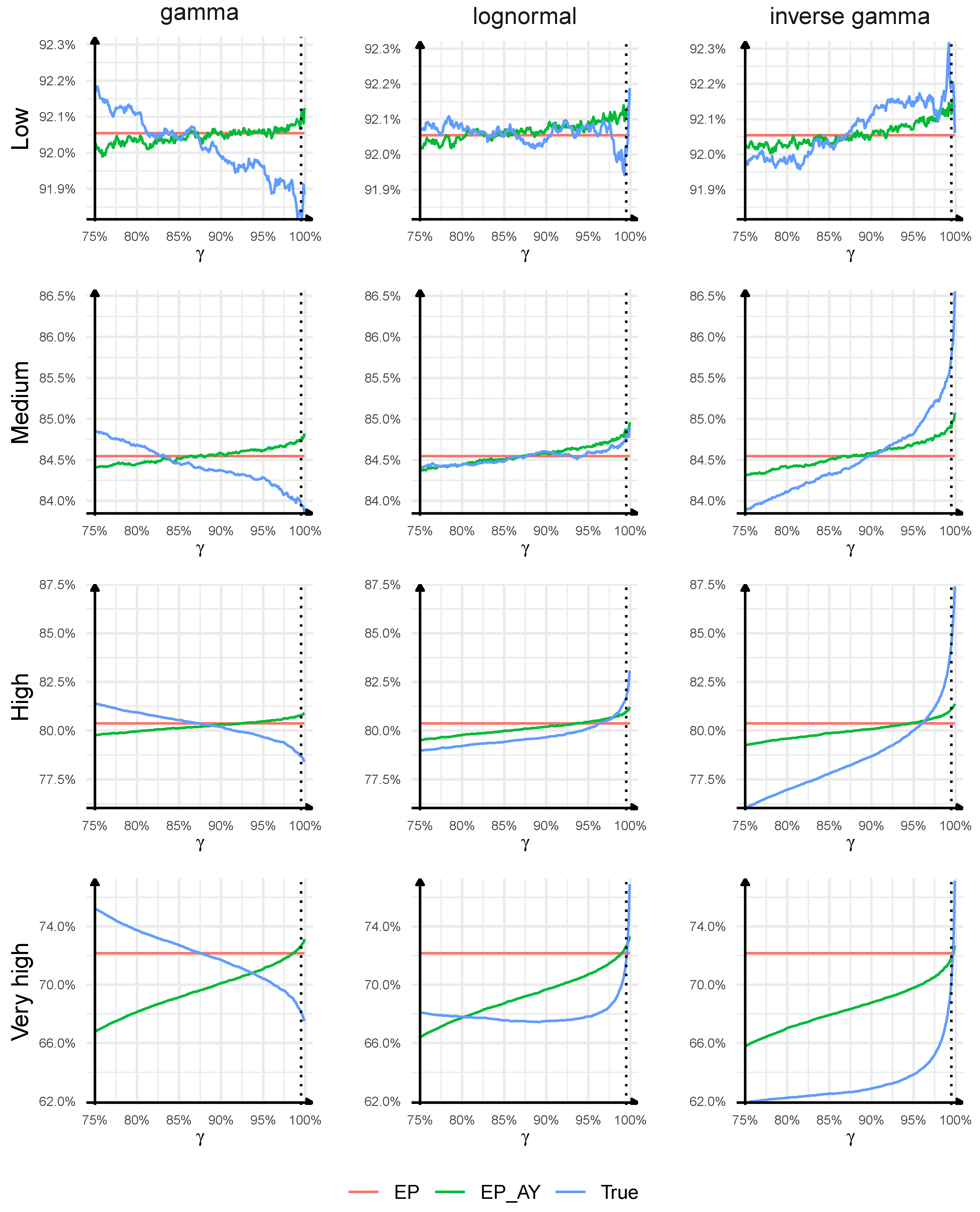
In Figure 3, we present the results for the models with the estimation error. In general, the qualitative conclusions concerning the emergence pattern formulas in reserve risk models with the estimation error are similar as in the case without the estimation error. However, we observe some interesting changes compared to Section 4.1.
It is clear that the true relation between the one-year reserve risk and the ultimate reserve risk described by the ratio (10) can vary significantly and depend on the confidence level, the characteristics of the claims development process in the loss triangle and the triangle type. For the triangles with lognormal and inverse gamma distributions, the ratio (10) is still an increasing function of the confidence level, except for very high triangle with lognormal distribution for which the ratio is slightly decreasing at first and then steeply increasing. The ranges of possible values of (10) for our confidence levels are now narrower than in the case without the estimation error—this time we get: – for high triangle with lognormal distribution, – for very high triangle with lognormal distribution, and – for the most extreme case of very high triangle with inverse gamma distribution. For the triangles with gamma distribution, we observe that the ratio (10) is still a decreasing function of the confidence level. Interestingly, the differences in the ratios are now much more visible than in the case without the estimation error. The range of possible values of (10) extends to – for high triangle, and to – for very high triangle. Only for low triangles is the true ratio of the one-year risk to the ultimate risk stable for all distributions and all confidence levels (close to in this case), which we also identify in Section 4.1.
By comparing the ratio (11) with (12), we come to the same conclusions as earlier that the linear emergence pattern formula applied to individual accident years does not lead to significantly different results from the linear emergence pattern formula applied to all accident years combined, except for very high triangles where the difference between the approaches becomes large, especially for low confidence levels.
We finally validate the adequacy of the linear emergence pattern Formula (5) in Chain Ladder models and its ability to approximate the one-year risk from ultimate losses. First, we observe that the curves determined by the emergence patterns (11) and (12) move downward compared to the case without the estimation error. This basically agrees with the intuition: if we investigate (12) with a single emergence factor, then the inclusion of the estimation error in a reserve risk model should have a larger impact on the mean square error of prediction for the ultimate loss than the one-year loss, which in turn decreases the emergence factor.4 Secondly, and less intuitively, the slopes of the curves determined by the true one-year loss (10) decrease for lognormal and inverse gamma distributions and increase for gamma distribution of individual development factors. These changes have a visible impact on the quality of the linear emergence pattern formulas. The quality of the approximation for low and medium triangles is better than in the case without the estimation error as the maximal misestimation errors, for all distributions and all confidence levels, are equal to and of the true one-year risk, respectively, for low and medium triangles. The reason for this improvement is that large misestimation errors observed in low and medium triangles with lognormal and inverse gamma distributions without the estimation errors decrease when the estimation error is included, and the misestimation errors for these triangles with gamma distributions do not increase significantly. For high triangles, for , the misestimation errors of the one-year risk are , , of the true one-year risk, respectively, for gamma, lognormal, and inverse gamma, while, for , the misestimation errors are , , , again for gamma, lognormal, and inverse gamma. For very high triangles, for all confidence levels considered, the maximal absolute misestimation error reaches , , for gamma, lognormal, and inverse gamma distributions. In comparison with the case without the estimation error, the misestimation error increases for the triangles with gamma distribution and decreases for the triangles with lognormal and inverse gamma distributions. One explanation for this change in the quality of the emergence patterns in our experiments might be that, when we include the estimation error, the ratios of the skewness of the one-year loss to the ultimate loss decrease and move closer to 1 for lognormal and inverse gamma distributions, whereas the ratios of the skewness of the one-year loss to the ultimate loss decrease and move away from 1 for gamma distribution, while we expect that the linear emergence pattern formula, at least (6), will work better, if the skewness coefficient of the one-year loss is close to the ultimate loss (as we have that ). We still observe that, for lognormal and inverse gamma distributions, the linear emergence pattern formula overestimates the Value-at-Risk measure for low confidence levels and underestimates VaR for high confidence levels and a reverse behaviour is observed for gamma distribution. Our examples still confirm that the linear emergence pattern Formula (5) may lead to a significant misestimation of the one-year risk in case of volatile, skewed claims development processes with long durations but it may offer a reasonable approximation of the one-year risk in case of low volatile, low skewed claims development processes with short durations. The impact of the tail of the distribution of the individual claims development factors on the performance of the linear emergence pattern formula is less intuitive as light-tailed distributions may have larger misestimation errors than sub-exponential/heavy-tailed distributions.
4.4. Approximations to the Outstanding Loss Distribution with the Estimation Error
We fit parametric distributions to the outstanding loss from the ultimate perspective and from the one-year perspective with the method of moments and validate the fit against the empirical distributions provided by our simulations from the previous section. We only consider the reserve risk models with the estimation error. As distributions of the outstanding loss we try: gamma, lognormal, inverse gamma. These distributions were suggested, e.g., by Dal Moro and Krvavych (2017); Mack (1994), for the outstanding loss from the ultimate perspective. As far as the one-year reserve risk is concerned, the Solvency II Directive postulates to calibrate the one-year reserve volatility based on either the Merz-Wüthrich formula, or historical changes in the run-off ratio (the ratio of the outstanding loss from the one-year perspective to the opening best estimate reserve) and to use a lognormal distribution to model the annual change in the run-off ratio; see CEIOPS (2010). Hence, gamma, lognormal, and inverse gamma distributions are natural choices in this study,5 and, despite their widespread use in reserve risk modelling, we are not aware of any validation report of their quality.
The distributions: gamma, lognormal, inverse gamma have two parameters which we fit to the expected value and the variance of the loss, calculated with the Mack and the Merz-Wüthrich formulas. We extend the class of possible distributions for modelling the outstanding loss by also testing the shifted versions of gamma, lognormal, and inverse gamma distributions. The third parameter of a shifted distribution is fitted by using the skewness coefficient of the outstanding loss. In the models with the estimation error, we estimate the skewness coefficients from the simulated losses.6 In case when the individual development factors are modelled with inverse gamma distribution, the skewness of the outstanding loss does not exist, as shown in Appendix A.1, and we only test non-shifted distributions.
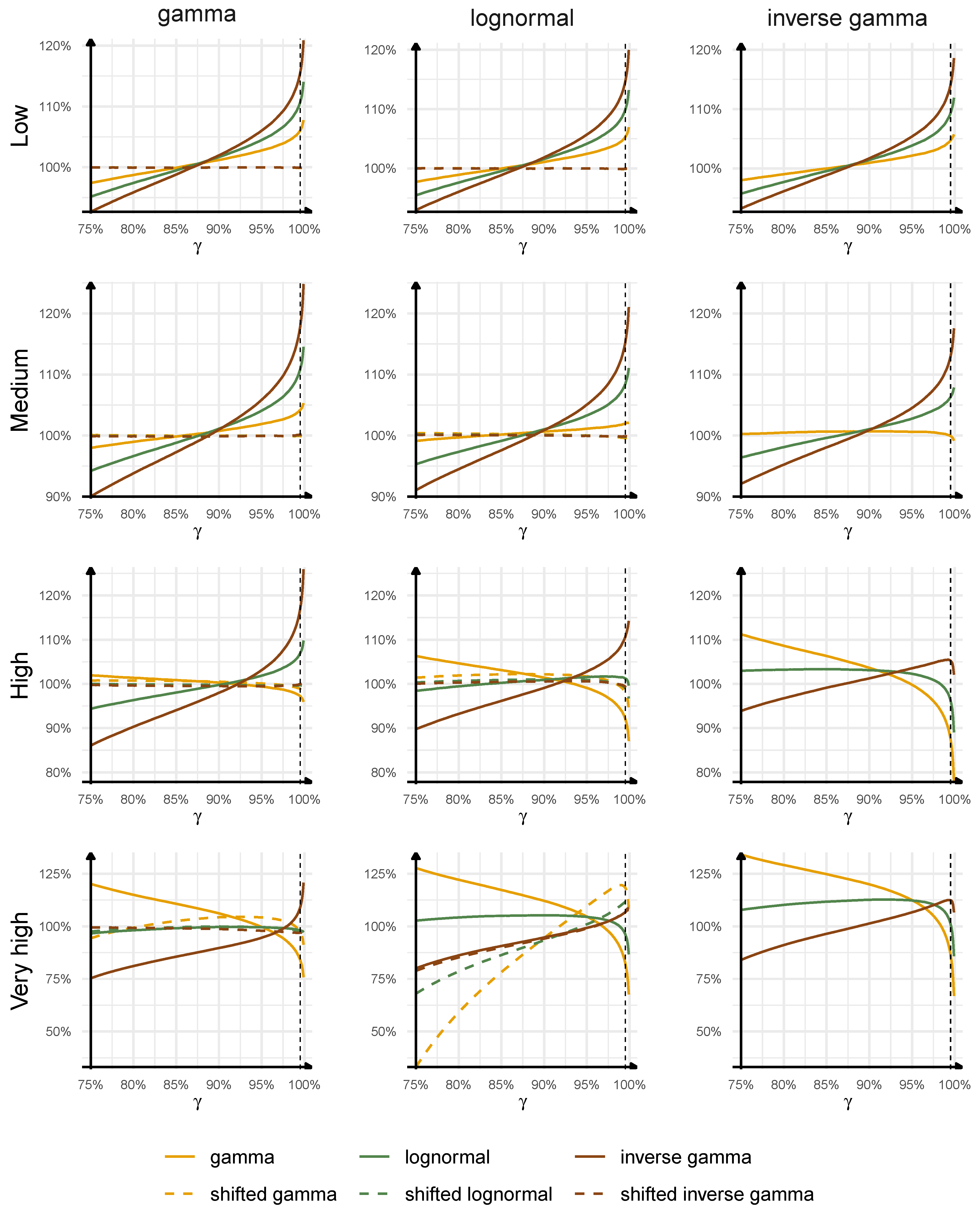
The results are presented in Figure 4 (from the ultimate perspective) and Figure 5 (from the one-year perspective). We analyse the quality of our approximations by studying the ratios:
where and are calculated using the fitted parametric distribution of the outstanding loss; hence, these terms describe our approximations, and and are estimated using the simulated sample of the outstanding losses, thus these terms being interpreted as the true quantile of the outstanding loss.
Let us focus on the distributions of the ultimate loss with the estimation error from the ultimate perspective, presented in Figure 4. We start with the non-shifted distributions. We may notice that the quality of the approximation and the choice of the best distribution depend on the triangle type and the confidence level. For triangles with shorter duration, lower volatility, skewness, and lighter tail of individual development factors, gamma distribution seems to provide the best approximation to the distribution of the outstanding loss. If we approximate the distributions of the outstanding loss for low and medium triangles with gamma distribution, the maximal misestimation of the true quantile of the outstanding loss is equal to at , and at , with the absolute misestimation errors being generally lower than . For triangles with longer duration, higher volatility, skewness, and heavier tail of individual development factors, lognormal distribution seems to outperform the others. If we approximate the distributions of the outstanding loss for high and very high triangles with lognormal distribution, the maximal misestimation of the true quantile of the outstanding loss is equal to at , and at , with the absolute misestimation errors being generally lower than . If we decide to use lognormal distribution to approximate the outstanding loss for low and medium triangles, then the maximal misestimation error is equal to at , and at , with the absolute misestimation errors being generally lower than in these two cases. This example presents that the choice of the best distribution is important and may have a significant impact on the quality of the results. The example with lognormal distribution is especially important for actuarial practice as this distribution is commonly used for approximations to the outstanding loss from the ultimate perspective; see Mack (1994). We can see here that, for low volatile, low skewed, light-tailed claims development processes with short durations, the use of lognormal distribution is conservative at high confidence levels; however, the overestimation of the true quantile can be as high as , whereas, at low confidence levels, the lognormal distribution can underestimate the true quantile by .
Interestingly, we can observe that the shifted distributions outperform the non-shifted versions for the triangles with gamma and lognormal distributions. Their better goodness of fit properties are a natural consequence of an additional parameter. For low, medium, and high triangles, the maximal absolute misestimation error of the true quantile of the outstanding loss, for all quantiles considered, is below for the triangles with gamma distribution, and below for the triangles with lognormal distribution, if the best shifted distribution approximating the outstanding loss is chosen. For very high triangle with lognormal distribution, the best shifted inverse gamma distribution only slightly improves the non-shifted inverse gamma. These examples clearly show that it might be beneficial to fit three-parameters distributions to the outstanding loss from the ultimate perspective as two-parameters distributions may misestimate significantly the true distribution.
The results for the outstanding loss with the estimation error from the one-year perspective, presented in Figure 5, are similar. Gamma distribution provides a better approximation to the outstanding loss for low and medium triangles, lognormal distribution provides a better approximation to the outstanding loss for high triangles. The new observation is that inverse gamma distribution provides the best approximation to the outstanding loss for very high triangles, but the quality of this approximation is poor in the most extreme triangle with inverse gamma distribution of individual development factors, as in the case with the ultimate perspective. It is worth pointing out that inverse gamma distribution now outperforms lognormal distribution for very high triangles, which was not observed for the outstanding loss from the ultimate perspective where lognormal distribution provides the best approximation in very high triangles. The reason for this change is that the skewness-to-CoV ratio (SC) for the outstanding loss from the one-year perspective is larger than the SC for the outstanding loss from the ultimate perspective in our examples and lognormal distributions cannot be fitted to large SCs without significantly increasing CoVs (for X with lognormal distribution, we have that , as stated in Dal Moro and Krvavych (2017)). We again point out that the use of lognormal distribution can lead to significant misestimation errors, both when it is used for low and medium triangles (outperformed by gamma distribution) and for very high triangles (outperformed by inverse gamma distribution). For the triangles with lognormal distribution of individual development factors, at , which is the most interesting confidence level for the one-year risk, the misestimation errors of the true quantile of the outstanding loss with the fitted lognormal distribution are equal to: , , , , respectively, for low, medium, high, and very high triangles. If we switch to the approximations of the outstanding loss with gamma distribution (for low and medium triangles) and inverse gamma distribution (for high and very high triangles), the misestimation errors decrease to: , , , for low, medium, high, and very high triangles. This example is again important as lognormal distributions are often used in practice for modelling the outstanding loss from the one-year perspective, as in CEIOPS (2010), and this may not be the best universal choice. Finally, the shifted distributions again outperform the non-shifted versions in approximating the outstanding loss and provide very good approximations with the maximal absolute misestimation error equal to across all cases, except very high triangle with lognormal distribution of individual development factors, if the best shifted distribution approximating the outstanding loss is chosen.
5. Conclusions
In this paper, we have investigated the relation between one-year reserve risk and ultimate reserve risk, without and with the estimation error, in Mack Chain Ladder models in a simulation study. We have demonstrated that the linear emergence pattern formula may misestimate the one-year risk and actuaries should apply emergence patterns with care when scaling the ultimate risk to the one-year risk. At the same time, the misestimation errors identified in our study seem not to be critical for loss triangles most often observed in actuarial practice. In a model without the estimation error, we have derived the true emergence pattern of the ultimate loss in a Mack Chain Ladder model and presented that it may differ from the linear emergence pattern formula. Finally, we have found that two-parameter loss distributions commonly used by actuaries, particularly the most commonly used lognormal distribution, may not be sufficient to model the outstanding loss from the ultimate and the one-year perspective and goodness-of-fit can be improved by fitting shifted versions of classical loss distributions.
Since our research and conclusions are based on synthetic loss triangles, we also performed similar calculations based on available real loss triangles, and we can confirm that the qualitative results are similar as the one presented in this paper. We have also tested the impact of two assumptions: the one concerning the initial exposure and its growth (by creating triangles following the same methodology as earlier but for different ) and the second about the deterministic pre-defined diagonal of the loss triangle (by creating triangles which lead to the same and , but have stochastic realizations). For both of these tests, there are naturally numerical differences in the results; however, the relation between the one-year and the ultimate reserve risk does not differ qualitatively.
Author Contributions
Conceptualization and methodology, M.S. and Ł.D.; writing—original draft preparation, M.S.; writing—review and editing, Ł.D. Both authors read and agreed to the published version of the manuscript.
Funding
This research is financially supported with grant NCN 2018/31/B/HS4/02150.
Conflicts of Interest
The authors declare no conflict of interest.
Appendix A
Appendix A.1. The Skewness Coefficient of the Ultimate Loss
We show how to calculate the third central moment of the ultimate loss in a model without the estimation error. Since the accident years are independent, . For a single accident year, we can use the well-know formula:
We now calculate the third raw moment of for .
- 1. has lognormal distribution: The parameters of the lognormal distribution are determined by CL1-CL3. From the formula for the third raw moment of lognormal distribution, we can deduce that
Let . By the law of iterated expectation and Markov property of the claims development process, we have that
We are able to calculate the third raw moments in an iterative fashion from up to .
- 2. has gamma distribution: We apply the same arguments, and we can derive
- 3. has inverse gamma distribution: The skewness of the ultimate loss does not exist. Let us choose and consider inverse gamma distribution with shape parameter and scale parameter for the next development period . Using moments for inverse gamma and CL1-CL3, we derive thatwhich are well-defined parameters of the distribution and the second moment of inverse gamma distribution is always finite. However, the third moment of inverse gamma distribution only exists for . Since the distribution of is not bounded from below, we may have on the last diagonal of the loss triangle or, with positive probability, in simulations of the development of the loss triangle. If this is the case, then CL1-CL3 imply that and the skewness does not exists. This property shows why the most volatile results are observed in our simulation study for inverse gamma distributions.
However, we can still choose a shifted inverse gamma distribution to approximate the distribution of the outstanding/one-year loss if its skewness is finite, which is the case if the individual development factors in the loss triangle are modelled with gamma and lognormal distributions. The method of moments now implies that (with being shift parameter).
where denote the expected value, variance, and skewness of the outstanding/one-year loss.
Appendix A.2. Additional Charts and Plausibility Checks of Our Simulations
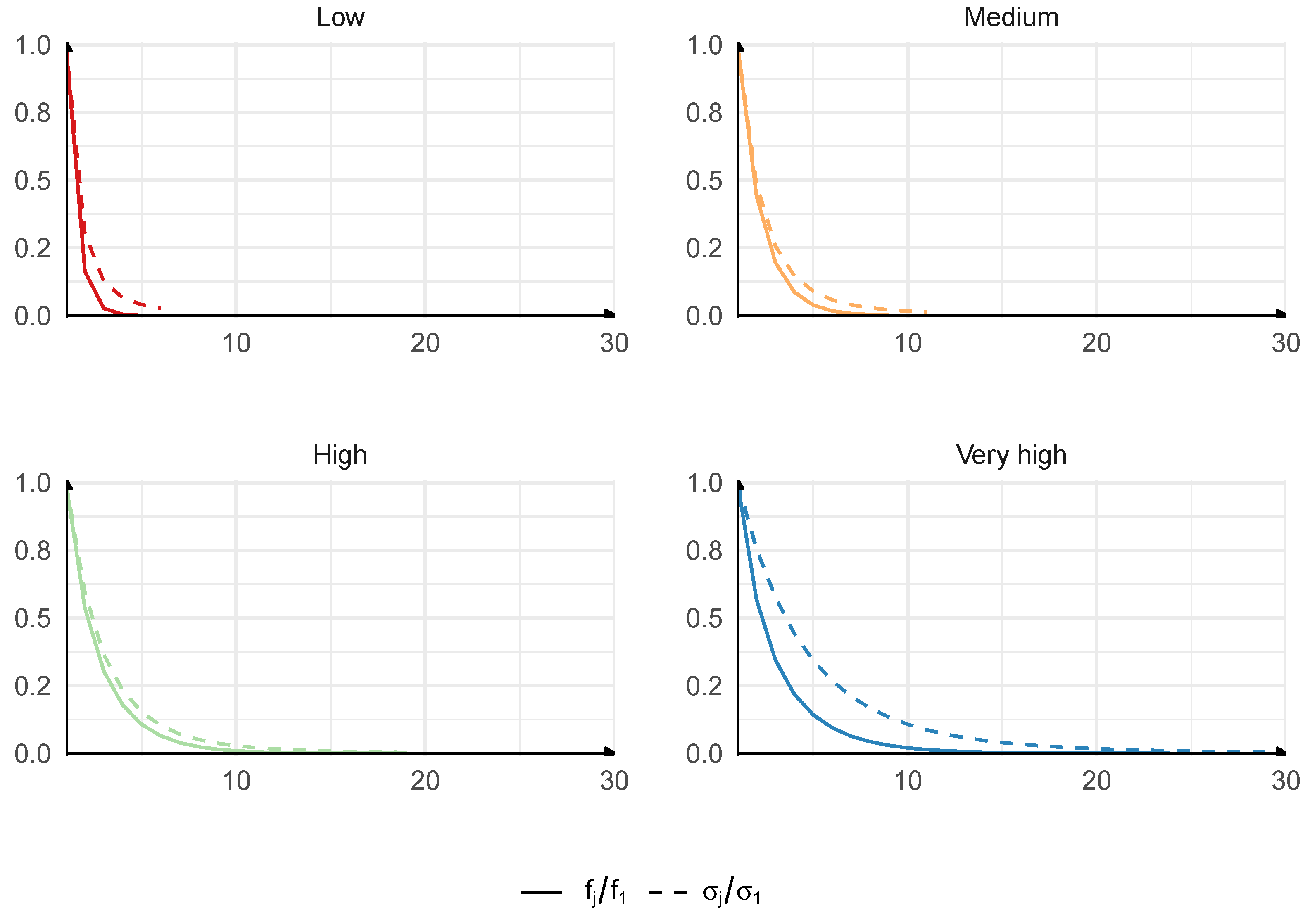
In Figure A1, we present the claims development factors and the log-volatilities used in our simulation study. Larger differences in , than for , are expected due to the fact that are defined in relation to the claims volume. In Figure A2, we observe that the claims development factors converge faster than the volatilities.
Figure A1.
Parameters and used in the simulation study.

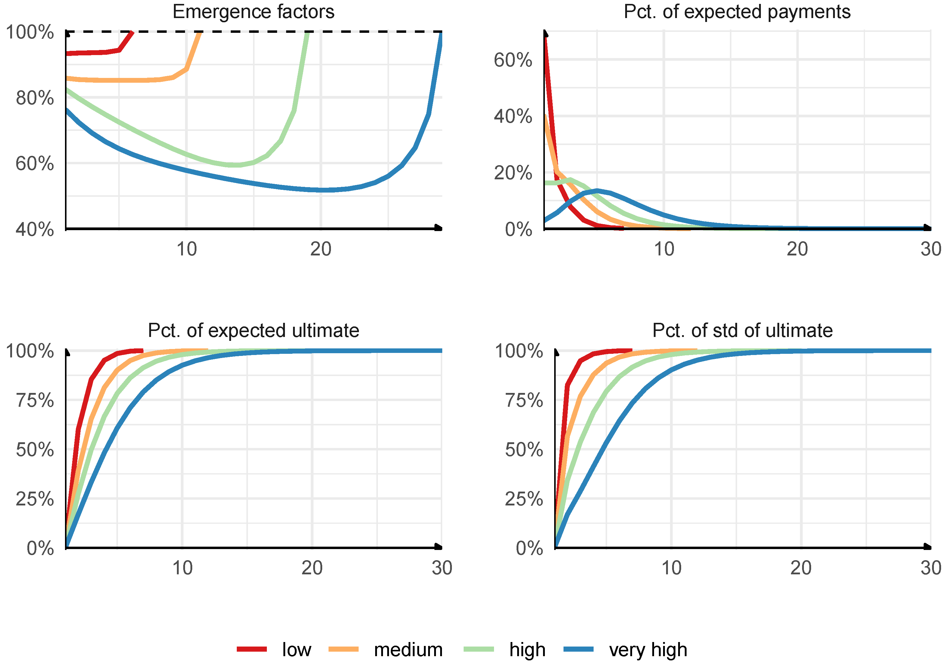
In Figure A3, we validate the results of our simulations without the estimation error. Similar plausibility checks were performed in the study with the estimation error. The values of the emergence pattern coefficients across accident years are U-shaped for all triangles, with lower values for higher lengths of tail, in line with England et al. (2012) and Scarth et al. (2020). The percentage of expected payments made in specific development year for a given accident year is monotonically decreasing for low and medium triangles, while, for high and very high triangles, it achieves the maximum value in later development years, which is in line with the observations in Guy Carpenter and Oliver Wyman (2014). The emergence of the expected ultimate loss and the standard deviation of the ultimate loss in calendar years is slower for triangles with longer tails, which is obvious.
Figure A2.
Convergence rates for the parameters and .

Figure A3.
Plausibility tests performed for the simulation study without the estimation error.

Additionally, we analyse developments of loss triangles by studying the maximum and the minimum of and quantiles of the simulated individual claims development factors across accident years and development periods (see Table A1). For the triangles: low, medium, and high, the simulated individual development factors are, most likely, in the range from to , which is acceptable from practical point of view. For very high triangles, we observe that the range of the simulated individual development factors is much larger, and they may attain 0 and go up to around 25. As commented in the paper, we constructed very high triangles so that they serve as the most extreme case observable in practice. The results for the case with the estimation error are very similar and are omitted.

Table A1.
The maximum of quantiles of order and minimum of quantiles of order across all accident years and development periods in the simulation study without the estimation error.
Table A1.
The maximum of quantiles of order and minimum of quantiles of order across all accident years and development periods in the simulation study without the estimation error.
| Gamma | Lognormal | Inverse Gamma | ||||
|---|---|---|---|---|---|---|
| Triangle | Max | Min | Max | Min | Max | Min |
| Low | ||||||
| Medium | ||||||
| High | ||||||
| Very high | ||||||
| 1 | The estimation error of the parameters is not quantified in the mean square error of prediction when we predict the loss with its expected value, and is also neglected in simulation models. |
| 2 | We also tested different exposures and the qualitative conclusions are the same. |
| 3 | By fixing the diagonal elements and the estimated claims development factors, we fix for each development period j. |
| 4 | We have also confirmed this behaviour for most of the tested empirical triangles; however, we have also found a few cases of triangles with a reverse behaviour— decreases when the estimation error is included. |
| 5 | These distributions are closed under scaling so we can model the run-off ratio or the outstanding loss. |
| 6 | The calculations of skewness coefficients in the models without the estimation error are discussed in Appendix A.1. |
References
- Bird, Chris, and Martin Cairns. 2011. Practical experiences of modelling one-year risk emergence. In GIRO Conference and Exhibition 2011. London: Institute and Faculty of Actuaries, Available online: https://www.actuaries.org.uk/system/files/documents/pdf/e07-bird-and-cairns-practical-experiences-modelling-one-year-risk-emergence.pdf (accessed on 15 June 2021).
- Buchwalder, Markus, Hans Bühlmann, Michael Merz, and Mario V. Wüthrich. 2006. The Mean Square Error of Prediction in the Chain Ladder Reserving Method (Mack and Murphy Revisited). ASTIN Bulletin 36: 521–42. [Google Scholar] [CrossRef] [Green Version]
- Carrato, Alessandro, Gráinne McGuire, and Robert Scarth. 2016. A Practitioner’s Introduction to Stochastic Reserving. London: Institute and Faculty of Actuaries. [Google Scholar]
- CEIOPS. 2010. Solvency II Calibration Paper. CEIOPS-SEC-40-10. Frankfurt am Main: Committee of European Insurance and Occupational Pensions Supervisors, April 15, Available online: https://www.eiopa.europa.eu/sites/default/files/publications/submissions/ceiops-calibration-paper-solvency-ii.pdf (accessed on 10 August 2021).
- Dal Moro, Eric, and Yuriy Krvavych. 2017. Probability of Sufficiency of Solvency II Reserve Risk Margins: Practical Approximations. ASTIN Bulletin 47: 737–85. [Google Scholar] [CrossRef]
- Dal Moro, Eric, and Joseph Lo. 2014. An industry question: The ultimate and one-year reserving. Uncertainty for different non-life reserving methodologies. ASTIN Bulletin 44: 495–99. [Google Scholar] [CrossRef] [Green Version]
- Delong, Łukasz, Mathias Lindholm, and Mario V. Wüthrich. 2020. Fitting Gamma Mixture Density Networks with E-M Algorithm. Available online: https://ssrn.com/abstract=3705225 (accessed on 15 June 2021).
- Delong, Łukasz, and Marcin Szatkowski. 2020. One-year premium risk and emergence pattern of ultimate loss based on conditional distributions. ASTIN Bulletin 50: 1–33. [Google Scholar] [CrossRef]
- England, Peter, Martin Cairns, and Robert Scarth. 2012. The 1 year view of reserving risk: The “actuary-in-the-box” vs. emergence patterns. In GIRO Conference and Exhibition 2012. London: Institute and Faculty of Actuaries, Available online: https://www.actuaries.org.uk/system/files/documents/pdf/b3-1-year-view-reserving-risk-actuary-box-vs-emergence-patterns.pdf (accessed on 15 June 2021).
- England, Peter, and Richard J. Verrall. 2002. Stochastic Claims Reserving In General Insurance. British Actuarial Journal 8: 443–544. [Google Scholar] [CrossRef]
- England, Peter, Richard J. Verrall, and Mario V. Wüthrich. 2019. On the lifetime and one-year views of reserve risk, with application to IFRS 17 and Solvency II risk margins. Insurance: Mathematics and Economics 85: 74–88. [Google Scholar] [CrossRef]
- Gisler, Alois. 2019. The Reserve Uncertainties in the Chain-Ladder model of Mack revisited. ASTIN Bulletin 49: 787–821. [Google Scholar] [CrossRef]
- Guy Carpenter Strategic Advisory, and Oliver Wyman Actuarial Consulting. 2014. Insurance Risk Benchmarks Research. Annual Statistical Review. Marsh&McLennan Companies. Available online: https://www.guycarp.com/content/dam/guycarp/en/documents/dynamic-content/Insurance_Risk_Benchmarks_Research_Annual_Statistical_Review.pdf (accessed on 15 June 2021).
- Harnau, Jonas. 2018. Misspecification Tests for Log-Normal and Over-Dispersed Poisson Chain-Ladder Models. Risks 6: 25. [Google Scholar] [CrossRef] [Green Version]
- Institute of Actuaries. 2002. Claims Reserving Working Party Paper, Graham Lyons, Chairman; London: Institute and Faculty of Actuaries. Available online: https://www.actuaries.org.uk/system/files/documents/pdf/lyons.pdf (accessed on 15 June 2021).
- KNF. 2020. Claims Development Factors According to Data from 31st December 2018. Urzaąd Komisji Nadzoru Finansowego (Polish Financial Supervisor); Warszawa: Departament Nadzoru Ubezpieczeniowego i Monitorowania Ryzyk, April 14. Available online: https://www.knf.gov.pl/?articleId=69507&p_id=18 (accessed on 15 June 2021).
- Mack, Thomas. 1993. Distribution-free calculation of the standard error of chain ladder reserve estimates. ASTIN Bulletin 23: 213–25. [Google Scholar] [CrossRef] [Green Version]
- Mack, Thomas. 1994. Measuring the Variability of Chain-Ladder Reserve Estimates. Arlington: Casualty Actuarial Society, vol. 1, pp. 101–82. [Google Scholar]
- Merz, Michael, and Mario V. Wüthrich. 2015. Modified Munich Chain-Ladder Method. Risks 3: 624–46. [Google Scholar] [CrossRef] [Green Version]
- Ohlsson, Esbjörn, and Jan Lauzeningks. 2009. The one-year non-life insurance risk. Insurance: Mathematics and Economics 45: 203–8. [Google Scholar] [CrossRef]
- Papachristou, Dimitris. 2016. The Emergence of Risk over One Year; London: Institute and Faculty of Actuaries. Available online: https://www.actuaries.org.uk/system/files/field/document/A9_The%20emergence%20of%20risk%20over%20one%20year_0.pdf (accessed on 15 June 2021).
- Peremans, Kris, Stefan Van Aelst, and Tim Verdonck. 2018. A Robust General Multivariate Chain Ladder Method. Risks 6: 108. [Google Scholar] [CrossRef] [Green Version]
- Rehman, Zia, and Stuart Klugman. 2010. Quantifying uncertainty in reserve estimates. CAS: Variance 4: 30–46. [Google Scholar]
- Robbin, Ira. 2012. A Practical Way to Estimate One-year Reserve Risk. Paper presented at CAS E-Forum, Denver, CO, USA, September 5–7. [Google Scholar]
- Röhr, Ancus. 2016. Chain ladder and error propagation. ASTIN Bulletin 46: 293–330. [Google Scholar] [CrossRef]
- Scarth, Robert, Saanya Jain, and Rocco Roberto Cerchiara. 2020. A Practitioner’s Introduction to Stochastic Reserving: The One-Year View. London: Institute and Faculty of Actuaries. [Google Scholar]
- Solvency II Regulation. 2015. Commission Delegated Regulation (EU) 2015/35 of 10 October 2014 Supplementing Directive 2009/138/EC of the European Parliament and of the Council on the Taking-Up and Pursuit of the Business of Insurance and Reinsurance (Solvency II). Brussels: European Parliament, Available online: https://eur-lex.europa.eu/legal-content/EN/TXT/PDF/?uri=CELEX:32015R0035&from=EN (accessed on 15 June 2021).
- Wacek, Michael G. 2007. The Path to the Ultimate Loss Ratio Estimate. Arlington: Casualty Actuarial Society, vol. 1. [Google Scholar]
- White, Stuart, and Simon Margetts. 2010. A Link between the One-Year and Ultimate Perspective on Insurance Risk. GIRO: 2010. London: Institute and Faculty of Actuaries, Available online: https://www.actuaries.org.uk/system/files/documents/pdf/workshop-d03-stuart-white-simon-margetts.pdf (accessed on 15 June 2021).
- Wüthrich, Mario V., and Michael Merz. 2008a. Stochastic Claims Reserving Methods in Insurance. Chichester: Wiley & Sons. [Google Scholar]
- Wüthrich, Mario V., and Michael Merz. 2008b. Modelling the Claims Development Result for Solvency Purposes. Arlington: Casualty Actuarial Society, pp. 542–68. Available online: https://www.casact.org/sites/default/files/database/forum_08fforum_21merz_wuetrich.pdf (accessed on 15 June 2021).
- Wüthrich, Mario V., and Michael Merz. 2015. Claims Run-off Uncertainty: The Full Picture. Swiss Finance Institute Research Paper No. 14–69. Zürich: Swiss Finance Institute, Available online: https://papers.ssrn.com/sol3/papers.cfm?abstract_id=2524352 (accessed on 15 June 2021).
Figure 1.
The ratios of Value-at-Risk measures for the one-year risk and the ultimate risk as a function of the confidence level—the case without the estimation error.
Figure 1.
The ratios of Value-at-Risk measures for the one-year risk and the ultimate risk as a function of the confidence level—the case without the estimation error.

Figure 2.
The true emergence pattern and the linear emergence pattern of the one-year loss—the case without the estimation error.
Figure 2.
The true emergence pattern and the linear emergence pattern of the one-year loss—the case without the estimation error.

Figure 3.
The ratios of Value-at-Risk measures for the one-year risk and the ultimate risk as a function of the confidence level—the case with the estimation error.
Figure 3.
The ratios of Value-at-Risk measures for the one-year risk and the ultimate risk as a function of the confidence level—the case with the estimation error.

Figure 4.
The ratios of Value-at-Risk measures for the outstanding loss estimated with parametric distribution and empirical distribution as a function of the confidence level—the case with the estimation error and the ultimate perspective.
Figure 4.
The ratios of Value-at-Risk measures for the outstanding loss estimated with parametric distribution and empirical distribution as a function of the confidence level—the case with the estimation error and the ultimate perspective.

Figure 5.
The ratios of Value-at-Risk measures for the outstanding loss estimated with parametric distribution and empirical distribution as a function of the confidence level—the case with the estimation error and the one-year perspective.
Figure 5.
The ratios of Value-at-Risk measures for the outstanding loss estimated with parametric distribution and empirical distribution as a function of the confidence level—the case with the estimation error and the one-year perspective.

Table 1.
CoV and SC measures of the outstanding loss from the ultimate perspective—the case without and with the estimation error.
Table 1.
CoV and SC measures of the outstanding loss from the ultimate perspective—the case without and with the estimation error.
| Without Estimation Error | With Estimation Error | |||||
|---|---|---|---|---|---|---|
| Triangle | CoV | SC | CoV | SC | ||
| Distribution | All | Gamma | Lognormal | All | Gamma | Lognormal |
| Low | ||||||
| Medium | ||||||
| High | ||||||
| Very high | ||||||
Table 2.
The quantiles of the distributions of the one-year loss derived with three methods—the case without the estimation error.
Table 2.
The quantiles of the distributions of the one-year loss derived with three methods—the case without the estimation error.
| Confidence Level | 75% | 80% | 85% | 90% | 95% | 99% | 99.5% |
|---|---|---|---|---|---|---|---|
| 78.3% | 78.6% | 79.6% | 80.5% | 81.1% | 83.4% | 83.8% | |
| 80.5% | 80.5% | 80.8% | 81.0% | 81.3% | 81.7% | 81.6% | |
| 78.0% | 77.8% | 79.1% | 79.8% | 80.4% | 83.5% | 84.0% |
Publisher’s Note: MDPI stays neutral with regard to jurisdictional claims in published maps and institutional affiliations. |
© 2021 by the authors. Licensee MDPI, Basel, Switzerland. This article is an open access article distributed under the terms and conditions of the Creative Commons Attribution (CC BY) license (https://creativecommons.org/licenses/by/4.0/).
Share and Cite
MDPI and ACS Style
Szatkowski, M.; Delong, Ł. One-Year and Ultimate Reserve Risk in Mack Chain Ladder Model. Risks 2021, 9, 152. https://0-doi-org.brum.beds.ac.uk/10.3390/risks9090152
AMA Style
Szatkowski M, Delong Ł. One-Year and Ultimate Reserve Risk in Mack Chain Ladder Model. Risks. 2021; 9(9):152. https://0-doi-org.brum.beds.ac.uk/10.3390/risks9090152
Chicago/Turabian StyleSzatkowski, Marcin, and Łukasz Delong. 2021. "One-Year and Ultimate Reserve Risk in Mack Chain Ladder Model" Risks 9, no. 9: 152. https://0-doi-org.brum.beds.ac.uk/10.3390/risks9090152
Note that from the first issue of 2016, this journal uses article numbers instead of page numbers. See further details here.