Investigation of Combining Logitboost(M5P) under Active Learning Classification Tasks


Department of Mathematics, University of Patras, 26500 Patras, Greece
*
Author to whom correspondence should be addressed.
Informatics 2020, 7(4), 50; https://0-doi-org.brum.beds.ac.uk/10.3390/informatics7040050
Submission received: 16 October 2020
/
Accepted: 29 October 2020
/
Published: 3 November 2020
(This article belongs to the Section Machine Learning)
Abstract
:Active learning is the category of partially supervised algorithms that is differentiated by its strategy to combine both the predictive ability of a base learner and the human knowledge so as to exploit adequately the existence of unlabeled data. Its ambition is to compose powerful learning algorithms which otherwise would be based only on insufficient labelled samples. Since the latter kind of information could raise important monetization costs and time obstacles, the human contribution should be seriously restricted compared with the former. For this reason, we investigate the use of the Logitboost wrapper classifier, a popular variant of ensemble algorithms which adopts the technique of boosting along with a regression base learner based on Model trees into 3 different active learning query strategies. We study its efficiency against 10 separate learners under a well-described active learning framework over 91 datasets which have been split to binary and multi-class problems. We also included one typical Logitboost variant with a separate internal regressor for discriminating the benefits of adopting a more accurate regression tree than one-node trees, while we examined the efficacy of one hyperparameter of the proposed algorithm. Since the application of the boosting technique may provide overall less biased predictions, we assume that the proposed algorithm, named as Logitboost(M5P), could provide both accurate and robust decisions under active learning scenarios that would be beneficial on real-life weakly supervised classification tasks. Its smoother weighting stage over the misclassified cases during training as well as the accurate behavior of M5P are the main factors that lead towards this performance. Proper statistical comparisons over the metric of classification accuracy verify our assumptions, while adoption of M5P instead of weak decision trees was proven to be more competitive for the majority of the examined problems. We present our results through appropriate summarization approaches and explanatory visualizations, commenting our results per case.
1. Introduction
Without a doubt, the last two decades have been characterized by massive production of data with regards to the fields of Computer Science (CS) and Artificial Intelligence (AI). Several real-life applications contribute to this phenomenon, operating as rich sources of data over all possible kinds: structured, semi-structured or unstructured [1,2]. We distinguish the next fields: social media platforms, economic transactions, medical recordings and Internet of Things (IoT) where Industry 4.0, constitutes a highly affected application coming from the latter field [3,4,5]. Although these applications offer advanced mechanisms for producing the necessary data under automated protocols and/or mechanisms, they still, in their majority, cannot address the data annotation under a similar and still accurate manner.
Therefore, the most widely known variant of Machine Learning (ML) algorithms, the supervised ones, do not stand as a proper solution for obtaining informative insights over the collected data, since the restricted number of annotated examples that may be acquired, even by a manual procedure, do not establish a sufficient training subset. Weakly Supervised Learning (WSL) and/or Partially Supervised Learning (PSL) approaches tackle this problem, trying to exploit the existence of the clearly larger amounts of non-annotated examples in order to mine useful information that might hide based on the aforementioned available annotated examples [6,7].
Different approaches of WSL and/or PSL approaches have been recorded in the related literature since their emergence. The common factor is the much smaller size of the labeled subset (L) against the corresponding unlabeled subset (U), while the most important points over which they differentiate are the following [8]:
- inductive/transductive approaches, where an explicit learning rule is formatted using the train set during the former one, trying to apply this on a distinct test set, while these two sets are both provided in advance during the latter;
- incomplete/inaccurate supervision, where both labeled and unlabeled examples are initially gathered regarding the first category, on contrast with the second one which is distinguished because of the noise that may govern the provided labeled examples, a fact that would cause intense deterioration on learning a specific task; and
- active/semi-supervised learning, where there is a straightforward separation of the approaches that need or demand human intervention so as to blend human’s knowledge into their total learning kernel for acquiring safer decisions instead of being based solely on a base learner’s predictions building a more automated learning chain but with greater risks.
Following the recipes of WSL/PSL approaches, the abundance of collected unlabeled data might act as a valuable source of information, reducing the negative effect of the difficulty on obtaining much labeled data, because of the inherent difficulties that take place on several domains. Ethical issues, scarcity of specific incidents and highly expensive labeling procedures are some of the obstacles that usually prevent us from handling successfully the creation of a large enough L per case [9]. However, based on the assumption that both L and U are produced from the same underlying data distribution , the connection between the conditional distribution and the marginal distribution could lead potentially to more accurate learning functions: , where stands for a typical example with N features while symbolizes the label that accompanies any such sample, being either known or unknown in the cases of L and U, respectively. Furthermore, through , we depict the space of the examples and the labels.
In this work, we aim to propose an accurate and robust batch-based inductive Active Learning (AL) algorithm for pool-based scenario, regarding the manner that the data are initially concerned. The base learner of the proposed AL algorithm is based on the adoption of an ensemble learner into its learning structure so as to cover efficiently the shortage of labeled data () along with the existence of a human oracle () that may provide us with trustworthy annotations. At the same time, a quite larger pool of unlabeled examples is available for mining its context [10]. Since the need for well-established predictions during the labeling stage of is one of the most crucial point during AL strategies, the exploitation of ensemble learners seems mandatory in order to capture better the insights of the examined data. Several recent works are also directed towards introducing ensemble learners into AL or other WSL variants, such as Semi-supervised Learning (SSL) [11], Cooperative Learning (CL) [12]—also known as AL + SSL [13,14]—or even Transfer Learning (TL) [15], while the field of supervised ensemble learners is still in bloom [16].
In our case, we prefer the adoption of the Logitboost ensemble learner, a product of the well-known procedure of generating ensemble learners through serially formatting a Generalized Additive Model (GAM), which does not prevent us from adopting additive tree models, as follows:
According to its strong theory, Logitboost manipulates the distribution of the training dataset based on the errors that occur during their categorization, where depicts the learning rounds of this iterative procedure [17]. Following the generic concept of boosting, during the training stage, we fit a number of learners which try to emphasize better on the instances that are misclassified. This is made through the weighting vector that enables the fitted learner to modify its decisions towards covering the most difficult cases based on their weight factors. After such rounds, we reach an iteratively boosted learning function, which has ideally transformed to a strong learner by continuously reducing the errors that the initial weak model and its previous variants faced.
Although the variant of AdaBoost is the most popular product of the boosting family algorithms, Logitboost actually constitutes a choice that may reward us compared to some defects that AdaBoost presents [18]. To be more specific, Logitboost uses a smoother weighting function than the default AdaBoost classifier, a fact that allows to address better the examples that are highly misclassified since the direction towards learning the proper mapping function per each learning round is not heavily affected by them. Instead, their importance does not overwhelm the corresponding importance of the examples with smaller misclassified errors, providing more robust confidence scores: . Taking into consideration that the choice of the most informative examples are more often than not selected through suitable metrics that depend on , such a behavior may be proven quite successful in practice [19,20]. Additionally, the convergence of the Logitboost scheme is not violated, as the general boosting procedure guarantees, since the logit-loss function which is described later is asymptotically minimized.
The favoring properties of the Logitboost ensemble learner have also been noticed in the related literature, although their cardinality is restricted. To be more specific, apart from using only univariate regressors inside this scheme, generalized functions could also be applied, increasing thus the total predictive ability but probably disrupting interpretability [21]. Otero and Sanchez proposed the use of descriptive fuzzy learners inside Logitboost, modifying slightly the usual structure of default fuzzy learners and overpassing the behavior of a similar fuzzy-based AdaBoost version [22], while a modification of the internal scoring mechanism based on distance from the decision regions using weak learners under Logitboost scheme was tested in [23]. Naive Bayes (NB) has also been combined appropriately with this scheme, improving its total performance against other popular variants of Bayesian Networks [24], while Logitboost’s operation was totally matched into the learning procedure proposed by Leathart et al., introducing Probability Calibration Trees (PCT) in the context of regression task, separating the input task space and fitting local predictors [25].
Logitboost autoregressive networks made use of the same scheme for modeling conditional distributions, offering a procedure that could be parallelized, exploiting the advantages of boosting ensembles for which the hyperparameters are clearly less than that of Neural Networks (NNs) and appeared to converge for several examined cases into same values, at least for the shrinkage factor [26]. More sophisticated multi-class expansions of Logitboost could further improve its applicability as it has been mentioned by the corresponding authors. This direction has been actually studied recently by some works, providing interesting expansions of the default multi-class operation of Logitboost scheme: Adaptive Base class (ABC) [27] and Adaptive One vs. One (AOSO) Logitboost [28].
Moreover, since the pool-based inductive AL strategies are inherently iterative procedures which are based on a few initially provided data, exploiting appropriately at least one for detecting the most informative —further analysis is presented on the next Section—the importance of obtaining accurate predictions is highly considered, but time limitations may occur when much complex learning models are embedded into these strategies. Trying to satisfy this trade-off under the Logitboost wrapper, we propose the use of M5P, a model tree regressor that tackles efficiently high-dimensional data since it builds linear models after having grown its preferred decision tree structure, taking advantage of its widely accepted decent learning performance over various scientific fields [29,30]. On the other hand, with the greedy manner under which Logitboost acts, although it is applied under a number of learning rounds (M), its total complexity does not differentiate heavier than other state-of-the-art classification algorithms [27]. Thus, its integration under AL strategies would not induce prohibitive time response in practice. Furthermore, since we maintain a regression tree as its base learner, both binary and multi-class classification problems can be addressed efficiently without inserting further modifications that would probably raise the computational complexity of the total algorithm.
Consequently, we propose the adoption of Logitboost(M5P) under pool-based AL classification problems, exploiting its favoring properties both for selecting informative unlabeled instances and for evaluating the final learning hypothesis, built into the gradually augmented L, based on the annotations that a powerful human oracle provides us. This combination has been recently examined in the scenario of SSL [31], presenting remarkable performance. For investigating the overall ability of Logitboost(M5P) under AL scenario, we examined 91 different datasets, separated into binary and multi-class under 3 different query strategies against the baseline strategy of Random Sampling (RS), comparing its performance against 10 other well-known learning algorithms as well as the default use of weak Decision Trees (DTs)—to be more particular, one-node trees [32]—into Logitboost, as it is usually met in the literature and related ML packages [33]. A further study tuning one hyperparameter of the proposed algorithm was also made, proving that its learning performance may still improve under suitable preprocess stages which however are not easy to trust under the existence of limited training instances.
More details regarding AL and a description of the proposed framework for examining the efficacy of Logitboost(M5P) in the case of an AL ecosystem are provided in the next two sections, along with the experimental procedure, the results and our comments, following the structure of the current journal. The last section summarizes our contributions and the pros and cons of our proposed combination, based mainly on our results, while future directions are posed.
2. Materials and Methods
The main reason that we resort to PSL methods is the coexistence of both L and U, while the amount of the latter (size(U)) is much larger than of the former (size(L)): [6]. One of the subcategories of PSL algorithms is AL, where Settles has demonstrated a great survey work on this kind of algorithms [10]. Trying not to present many details, we highlight the most important parts of such a learning strategy.
First of all, we employ a probabilistic classifier (f) acting towards two different directions: searching for the most compatible s and evaluating the final model after a predefined number of iterations is reached or until any other set stopping criterion is satisfied. The first part is handled by exploiting a proper sampling Query Strategy (QS) which defines a specific criterion or metric , so as to measure the informativeness or the utility of all the available s. In order to detect the most convenient of them for creating a batch (B) of potentially informative s so as to increase the learning ability of the total AL learning procedure, we select the top b highly ranked instances:
where is actually a subset of the applied U during each iteration. The second is resolved through employing one or more human oracles or sources of information, like known crowdsourcing platforms, e.g., Amazon Mechanical Turk and CrowdFlower [34].
This means that, after having detected the B, we ask the available to assign the corresponding label based on its knowledge background. Then, we merge the pairs of {B, } with the initially collected L during the first iteration or the current version of L for next iterations Liter, where iter depicts the current iteration. Then, we refine f and repeat this procedure until a terminating condition is satisfied. In contrast with pure SSL approaches or in general with the wide spectrum of WSL approaches, the terminating condition of the empty U pool is not a realistic one here, since this would demand much effort on the side of the human factor. The participation of the latter introduces several trade-off situations that should be considered carefully.
According to the related literature [20], there are 3 general kinds of QS models on the field of pool-based AL and a group of hybrid ones that combine more than one strategy:
- heterogeneity-based,
- performance-based,
- representativeness-based, and
- hybrid ones,
where more details are provided in [35]. A quite important research orientation of the related community is the proposal of a new QS, either introducing new metrics which may measure a behavior that seems more favorable for specific tasks [36,37] or trying to capture better the reasoning of some choices made by similar methods [38]. One representative work related to this last category is the work of Vu-Linh Nguyen et al. [39], exploring further Uncertainty Sampling (UncS) QS, discriminating this into epistemic and aleatoric sampling strategies, highlighting their differences and proposing the first variant as more promising.
We actually adopted UncS in our AL framework, which tries to distinguish the instances for which the applied learning algorithm being trained on Liter is less confident. For a binary problem, such an instance would induce . This strategy favors time-efficient solutions for the majority of ML algorithms because its time complexity demands a training stage of f over Liter and an evaluation stage of Uiter. Since the cardinality of the former is smaller than the latter, especially for low labeled Ratios (R)—where R is defined as the ratio of the initial L’s cardinality against the total amount of both L and U—the needed computational resources can be bounded based on the computational complexity of the base learner. Of course, the size of the batches (b) and the number of executed iterations (k) also play important roles.
In order to investigate the efficiency of Logitboost(M5P) under UncS, we employed 3 separate metrics inside this wrapper strategy, comparing them each time with the baseline of RS, where no sophisticated criterion was assessed for selecting the participant of each batch but a random pick took place before the corresponding batch was provided to . This strategy comes with no time costs during the mining of U. This means that any examined QS should outreach this performance for being qualified as a valid one for the concept of AL. The relationship of each of the utilized (Least Confident: LConf, Smallest Margin: SMar and Ent: Ent) is given here:
where is the confidence of the base learner on the examined , while Equation (5) computes the difference between the two most probable classes of the same so as to return the most compatible choice from the available into U.
With regards to the proposed base learner, Logitboost(M5P), more details are given here. Logitboost is an additive logistic regression algorithm that can be seen as a convex optimization problem. An additive model, like simple linear models or regression trees, for solving a binary problem has the function of the following form:
where m is the number of classifiers, is the constants to be determined and is the chosen base functions along with their internal parameters . Assuming now that is the mapping that we need to fit our strong aggregate hypothesis and is the separate weak hypotheses, then the two-class boosting algorithm is fit by minimizing the next criterion:
where y is the true class label and is the voting margin term [40], while denotes the expected value.
Adopting the negative binomial log-likelihood does not affect the minimizer of Equation (8) compared with the typical boosting function, enabling at the same time a smoother weighting of examples for which predictions of Logitboost learner are far away from the discriminating decision threshold, constituting a great asset. This procedure takes place using the Newton-like steps, a more complicated optimization process than in the case of exponential loss function of AdaBoost algorithm. However, this fact does not affect the ambition of minimizing the set loss function during the training process.
Regression trees are known for their ability to deal efficiently with large datasets in terms of both features and instances, added to their simplicity and robustness [41]. The M5P regressor is a recreation of M5 algorithm [42], where the portion of the dataset that reaches the leaf is classified by a linear regression model stored in each branch of the tree. For the dataset split, certain attributes are chosen using the standard deviation error (SDR) as a criterion for the best attributes to split the dataset at each node. The chosen attribute is the one with the maximum expectation to error reduction:
where refers to the subset of examples that have the ith result of the potential test and refers to the standard deviation of its argument. The stopping criteria is either the number of remaining instances to reach a certain number or a very small change in class value.
The successful competition of M5P against other regression trees or other conventional ML learners has been stated in recent literature [30,43,44]. Its exploitation under the wrapper scheme of Logitboost could lead to a robust classifier that operates on the field of AL, both for choosing informative instances and for providing remarkable classification performance. Moreover, possible inaccurate predictions that would appear because of either a shortage of that covers the total range of the output values or weak indicators originally existing in the feature space of a dataset could be alleviated by the smooth weighting function that Logitboost applies, avoiding the overfitting phenomena that might discard its decisions [45].
The last mechanism that needs to be described before more technical details of the experimental procedure is the increase in L during the iterative process of a typical AL environment. To be more specific, the queried instances (b) are chosen in batches. The size of each batch relies on the size of the initial labeled set of each dataset and the number of predefined iterations (k). This happens because we adopted an augmenting strategy that aims to double the size of the labeled instances at the final (kth) iteration of the experiment. According to this concept, the steady value of the parameter b per dataset is computed as follows:
Thus, to execute a complete AL experiment fairly, we adopted a flexible process for which the pseudocode is placed in Algorithm 1. Initially, we start with size(L) collected labeled instances, and before the final evaluation, 2*size(L) instances are gathered, where the additional labeled instances have been assigned with pseudo-labels by after their selection through the combined interaction of any chosen QS and our selected base learner. During each iteration, a batch B that consists of b instances is extracted from the U subset and is added along with the decisions of the employed into the current L subset. For the evaluation process, a test set is used to examine the accuracy of the Logitboost(M5P), which is now trained on the augmented labeled set through the process of the AL. The total procedure is as follows:
| Algorithm 1Active learning scheme |
| 1: Mode: |
| 2: Pool-based scenario over a provided dataset D = Xn x N ⋃ Yn x 1 |
| 3: xi—i-th instance vector with N features xi: <x1, x2, … xN> ∀ 1 ≤ i ≤ n |
| 4: yi—scalar class variable with yi ∊ {0, 1} or unknown ∀ 1 ≤ i ≤ n |
| 5: n—number of instances n = size(L) + size(U) |
| 6: B—batch of unlabeled samples that are labeled per iteration |
| 7: Input: |
| 8: Liter (Uiter)—(un)labeled instances during the iter-th iteration, Liter ⊂ D, Uiter ⊂ D |
| 9: k—number of executed iterations |
| 10: base learner—the selected classifier |
| 11: QS(metric)—the selected Query Strategy along with its embedded metric |
| 12: Preprocess: |
| 13: b—size of batch B computed by Equation (10) |
| 14: Main Procedure: |
| 15: Set iter = 1 |
| 16: While iter < k do |
| 17: Train base learner on Liter |
| 18: Assign class probabilities over each ui ∊ Uiter |
| 19: Rank ui according to QS(metric) |
| 20:Select the top-b ranked ui formatting current B |
| 21: Provide batch B to human oracle and obtain their pseudo-labels: |
| 22: Update L: Liter+1 ← Liter ⋃ {B, } |
| 23: Update U: Uiter+1 ← Uiter\{B} |
| 24: iter = iter + 1 |
| 25: Output: |
| 26: Train base learner on Lk for predicting class labels of test data |
3. Results
More technical details are revealed in this section to both describe better the volume of our executed experiments trying to better clarify the importance of the Logitboost(M5P) as a robust inductive learner under the AL concept and to favor the reproducibility of the total experimental procedure. Therefore, we firstly describe the basic properties of the examined datasets, providing later the details of the experimental phase regarding mainly the parameters of the compared algorithms as well as the open-source platform that we utilized to execute them. Finally, we share a link with all the produced results and visualizations due to lack of space.
3.1. Data
All of the mined datasets come from the well-known University of California-Irvine (UCI) repository [46]. The next two figures represent their formulation, having separated them based on the number of class into binary and multi-class datasets. Thus, in Figure 1, the third column—depicting the number (#) of classes—contains recordings equal to 2 for all datasets, while in Figure 2, this parameter varies from 3 to 28 for our case. The last column depicts the ratio that the class with the most instances (majority class) and the class with the least instances (minority class) capture against the rest ones. In the former case (Table 1), these two values sum up to 100%, while in the latter case, we added the corresponding ratios of the two most minor classes, since some datasets contain some extremely rare classes, and depicting only their contribution to the total instances would be neither convenient nor informative for the reader. Therefore, the last column of all datasets with exactly 3 classes presented in Table 2 sums up also to 100% (contribution of largest class/contribution of the two most minor classes), while for the rest multiclass datasets, these values are not constrained. The fact that the majority of the datasets are imbalanced sets some kind of difficulty over the examined AL algorithms, but this property at the same time is met in the most remarkable challenging real-life problems. Thus, no preprocess stage was applied for balancing the datasets based on the cardinality of their classes. One exception is the “texture” dataset, which contains 11 classes with exactly 500 instances per each class, leading to perfect balance.
As it concerns the rest of the information that characterizes the structure of our examined datasets, we mention that their cardinalities range from 57 (“labor”) to 67,557 instances (“connect-4”), while their feature space ranges from 2 (“banana”) to 90 (“movement-libras”), covering thus a wide spectrum of cases regarding these two properties. Additionally, the 5th column distinguishes and counts accordingly the number of categorical and numerical features. Analogous to their participation, there are datasets for which features are related solely with one category (numerical or nominal) or with both of them, usually called mixed.
3.2. Active Learning Components
3.2.1. Classifiers
In order to investigate properly the distinguishing ability of the proposed combination of Logitboost with the M5P under the AL concept, 7 different classifiers have been selected so as to operate under the same AL framework, as this was combined in Algorithm 1. Some brief details of these classifiers along with their original references are recorded here:
- k-Nearest Neighbors [47], the most representative classification algorithm from the family of lazy learners, also referred to as an instance-based algorithm since it does not consume any resources during the training stage. Instead, it computes based on appropriate distance metrics the k-nearest neighbors of each test instance and exports its decision through a simple majority vote about the class of the latter one. Three different variants of this algorithm were included: 1-NN, 3-NN and 5-NN, increasing the value of the k parameter;
- Decision Trees (DTs) [48], where J48 and Random tree algorithms from this category were preferred. The first one constitutes a popular implementation of C4.5 generating a pruned variant that exploits Gain Ratio to determine how to split the tree, while the second one considers just a randomly chosen subset of the initial feature space before growing an unpruned decision tree. Logistic Model Trees (LMT) [49] was also employed as a powerful ensemble algorithm. Based on this, a tree structure is suitably grown, but proper logistic regression models are built at its leaves, exploiting in this manner only the most relevant attributes;
- JRip [50], a rule-based learner that tries to produce rules so as to capture all the included instances into the provided training set;
- Naive Bayes (NB) [51], a simple Bayesian-based method that assumes that all the features inside the original feature space are independent. Although this assumption seldom holds, especially in real-life cases, this generative approach has found great acceptance at the literature; and
- AdaBoost (Ada) [18], the most popular boosting algorithm that minimizes exponential loss.
As all the mentioned algorithms as well as the proposed combined Logitboost(M5P) learner were considered, they were mined from the Waikato Environment for Knowledge Analysis (WEKA) environment [33], keeping the default parameters of all their original implementations, enforcing the reproducibility and conducting fair comparisons.
3.2.2. Experiment Details
Considering the evaluation of our results, we applied a 3-fold-cross-validation procedure (3-CV) where the 2 out of three folds were held for the training data and the rest was for testing. Afterwards, the training data were split to L and U under 4 different R values: 5%, 10%, 15% and 20%. After executing 15 iterations, the size of the labeled data compared to the total training data increased to 10%, 20%, 30% and 40%, respectively. This procedure was repeated 3 times per case, executing a 3 × 3-CV evaluation stage. For implementing our pool-based experiments with the UncS and the aforementioned metrics, along with the RS strategy, we used the ‘Java Class Library for Active Learning’ (JCLAL) library, a Java-based library that interacts directly with the WEKA facilitating the use of the algorithm classifiers in this framework [52]. Furthermore, we conducted the next comparisons (the proposed learner versus 1. simple or 2. ensemble learners) regarding the classification accuracy (Acc%) metric, verified later by a nonparametric statistical comparison process:
- Logitboost(M5P) vs. 1-NN vs. 3-NN vs. 5-NN vs. J48 vs. JRip vs. NB vs. RandomTree
- Logitboost(M5P) vs. Logitboost(DStump) vs. Bagging(J48) vs. Ada(DStump) vs. LMT
The second set of comparisons is an investigation between the learning behavior of the proposed combination of M5P under the Logitboost scheme with the default Logitboost, which exploits the Decision Stump algorithm (DStump) [32], a simple one-node tree that discriminates each example using only one feature which acts as the root of this simplified tree. Additionally, the well-known Bagging scheme along with the J48 algorithm has been also examined for consistency reasons, comparing our proposed base learner with another ensemble approach, based again on DTs [53,54] along with the Ada and LMT learning approaches that have found great acceptance in practice.
3.3. Figures, Tables and Schemes
Here, we record the results of the smallest R-based scenario (R = 5%) only for the UncS(Ent) QS. We provide two tables for each comparison setting, separating thus on binary and multi-class datasets (Table 3, Table 4, Table 5 and Table 6).
Due to the volume of produced results and to maintain a balance between the extension of the presented results and the main body of the rest manuscript, our included tables and figures present our results only for a small portion of our total experiments. The following link contains all results: http://ml.math.upatras.gr/wp-content/uploads/2020/10/MDPI_Informatics_AL_Logitboost_M5P.7z.
In the preceding 4 tables, we highlighted the best value per dataset (row) achieved by all the included algorithms (columns) in bold format to facilitate visualization of these results. However, some implications occurred during our experiments and we have to record them here. Initially, it has to be mentioned that the JRip algorithm did not manage to export decisions for the majority of the datasets under the SMar metric. This behavior is recorded because of JRip’s inherent inability to produce rules for all the existing classes, especially when the training data are not sufficient. Thus, we have removed this algorithm from the corresponding files, but it is still included for the other QSs. Furthermore, the LMT algorithm as well as Ada(DStump) did not manage to export predictions for 20 (15 binary and 5 multi-class) datasets, which made us remove all of them from the second set of comparisons: the proposed algorithm versus the ensemble ones.
Continuing with our results, in order to present some better insights into the total experiments, we have gathered the victory frequencies for these two cases into Table 7 and Table 8, separated internally depending on the number of the existing classes and summarizing the performance per learner for all the examined R-based scenarios and the distinct query strategies applied. We have ignored the RS case, since this acts as the baseline in the AL concept, but we have taken into consideration this strategy in the statistical comparisons that follow. In the aforementioned case of JRip under UncS(SMar) strategy, we did not record any value since it has been rejected by this kind of experiments.
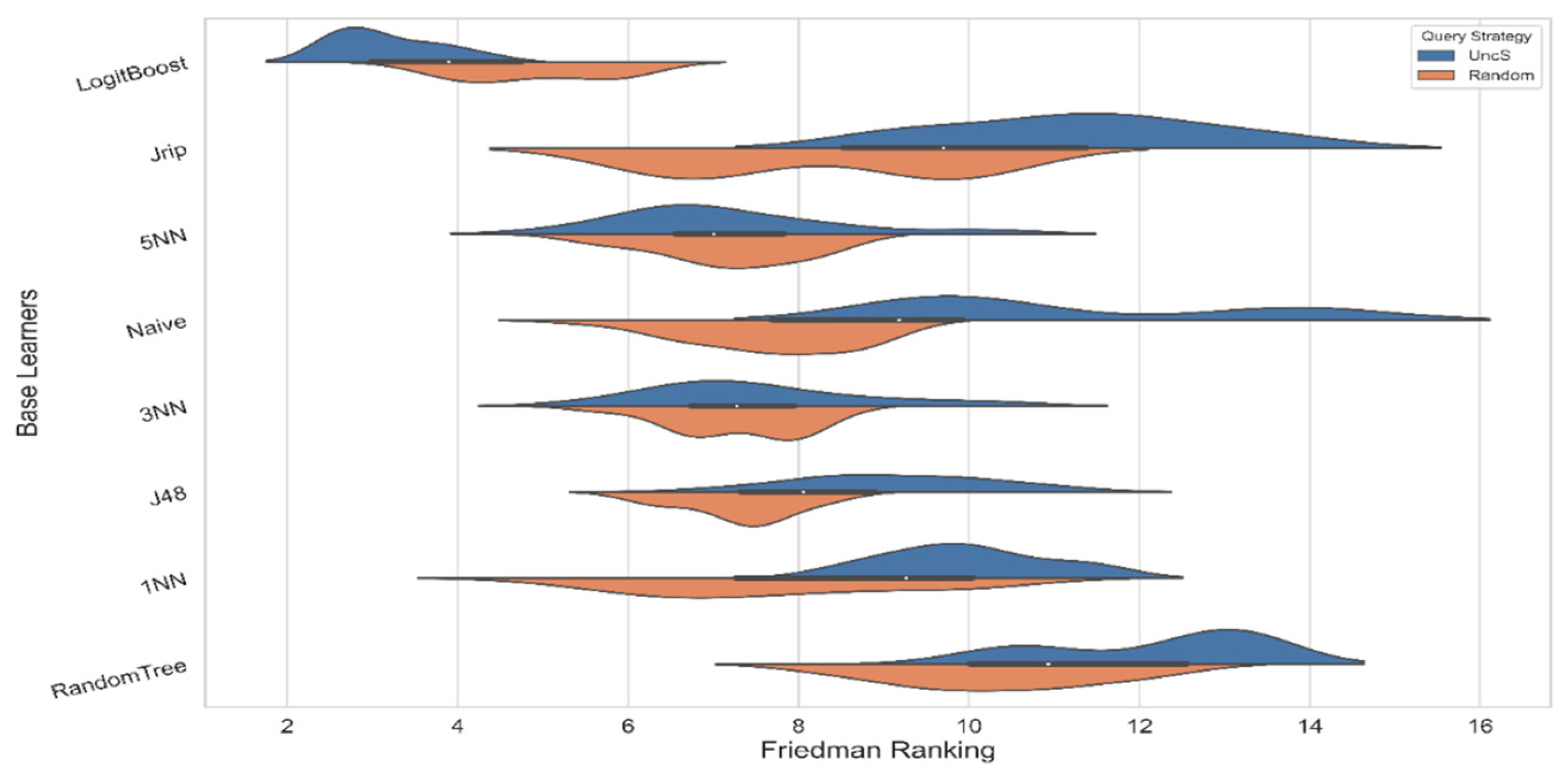
Considering the statistical comparison of the first part of the results, we have applied the well-known nonparametric Friedman test, which examines if the null hypothesis about the similarity of the participating algorithms as it considers their performance holds [55]. Since both Friedman and Iman–Davenport statistics highly favored the rejection of the null hypothesis, a proper post hoc test was applied to investigate further the statistical importance of the acquired results. In our case, the post hoc of Nemenyi was selected using an alpha level parameter equal to 0.05 [56]. The value of the critical difference (CD) that should be overpassed between the learning behavior of two algorithms for being considered as statistically different is 1.21. The next figure depicts the achieved scores per base learner for both the binary and multi-class datasets, discriminating the performance of the 3 examined metrics under UncS against the RS. A violin plot was chosen.
Regarding the second part of the experiments, a more targeted comparison was made to verify the predictive ability of the proposed variant of Logitboost against its default setup, as has been implemented on WEKA API, which actually uses a one-node tree as a weak learner, while the other 3 ensemble learners have been included. Therefore, we applied a twofold comparison, examining their efficacy on both the binary and multi-label datasets, following the same statistical verification as previously. We have already measured the frequency of the best achieved performance for all examined datasets per ensemble learner, QS and R-based scenario in Table 9, while in Table 10, we present the corresponding Freidman rankings. For acquiring better insight of the relative importance of the learning performances of this kind of comparison, we recorded the corresponding statistical ranking per separate R-based scenario.
Indeed, we can verify that different behaviors are recorded in the largest R-based scenario compared with the rest ones during the binary datasets, a fact that would not have been noticed under an average of the separate rankings, being merged and leading to erroneous conclusions. Despite this fact, the underlying CD value for this set of experiments is equal to 0.568, a score that settles that the proposed approach is significantly superior against the other examined algorithms under the same AL framework in 5 out of the 8 cases.
Meanwhile, the next 3 figures depict the performance of the Logitboost(M5P) against its 4 ensemble opponents for the 9 largest datasets, across both kind of datasets, through compatible error-bar plots that summarize the performance on each evaluation during the 3-fold-CV process as well as the corresponding average value for each iteration.
4. Discussion
In this section, we briefly discuss the obtained results from both comparisons to summarize the overall results and to perceive better the assets of the proposed AL approach that is based on the combination of Logitboost scheme with the M5P regressor. First, application of Logitboost under AL has not been recorded in the literature in contrast to several other ML models [57]. Consequently, it was reasonable to adopt a common AL framework to make fair comparisons with the selected approaches that are based on state-of-the-art algorithms during both of the examined settings. Thus, no tuning stages were inserted into the learning pipeline. The total experimental procedure was conducted regarding 4 different values of the R (%) parameter, trying to investigate further the behavior of all the examined approaches, assuming that the human oracle did not introduce any noisy decisions at all. Thus, we do not insert noisy decisions during augmentation of the initial labeled set, which shifts the responsibility of selecting informative instances to the learning ability of the base learner per case. Additionally, we are more interested on the lowest R-based scenarios since they constitute more realistic simulations of real-life WSL problems.
From the accuracy score recorded in Table 3 through Table 6, we can see that the proposed combination highly outperformed its rivals on the majority of the 91 datasets. The aggregated number of victories for both sets of comparisons—versus simple and ensemble base learners—have been placed in Table 7 and Table 8, where the proposed set managed to capture the best performance in 774 cases out of 1112 (69.6%) against 6 approaches and in 499 out of 866 cases (57.6%) against 4 approaches. Moreover, its defects seem to appear on specified datasets (e.g., “iris” and “post-operative” from binary datasets as well as “heart-h”, “saheart” and “newthyroid” from multiclass ones). The structure of these datasets should be examined further, but probably a tuning stage of Logitboost scheme, for which the parameters could be expanded because of the presence of the internal regressor, might lead to better performance against algorithms like kNN or learners that are based on DTs, either individually or under an ensemble fashion.
As it concerns the first experimental scenario, the distribution of the number of victories of the proposed AL approach was similar across the different query strategies and the labeled ratios, denoting its general efficacy against the other approaches. The 3 distinct kNN learners also performed cumulatively 243 victories, constituting a useful proof about their robustness despite the restricted number of labeled examples [58]. On the other hand, the performance of NB as a base learner was disappointing, affected by the aforementioned shortage of numerous initial examples since it did not record any victory.
During the second and, of course, more challenging scenario against ensemble base learners, the proposed algorithm was again more competitive and outperformed the rest in the majority of the grouped experiments. However, LMT-based approaches managed also to score several winning accuracies per dataset, especially in binary problems when larger R-based experiments were conducted. In fact, LMT expands the Logitboost procedure internally into its main learning kernel but, at its final stage, exploits only a subset of the initial feature space so as to build its logistic model. This property seems favorable for the aforementioned case, as the statistical rankings placed in Table 10 prove. Specifically, for binary problems, the proposed algorithm performed significantly better behavior than the LMT-based AL approach only for the case of R = 5%, while for the next two comparisons, no statistical difference was recorded, ranking Logitboost(M5P)-based approaches in first with a slight lead, while in the last scenario, where R = 20%, the LMT significantly outperformed the proposed one. However, in multi-class problems, this behavior was not repeated. This kind of result possibly denotes the existence of noisy features that highly affect binary problems and/or highlights the overfitting phenomena that Logitboost may face when outliers are inserted into its training stage.
Returning to the first set of experiments, a statistical comparison was executed for verifying the results obtained from the examined query strategies against also the baseline of random sampling. Figure 2 captures the performance per district learner, where the proposed base learner recorded a statistically significant behavior against its baseline as well as the rest of the AL approaches, being ranked always as the best across all the conducted scenarios. It is remarkable that the RS(Logitboost(M5P)) approach managed also to outreach the other simple algorithms on average, proving the overall predictive ability of the proposed ensemble learner. This last note highlights also the implications that may occur when ranking the available unlabeled examples, a fact that may deteriorate the total learning behavior since the less informative the selected instances are labeled, the more redundancy that occurs in the gradually augmented training subset.
Discussing again the second experiment setup, a similar procedure was implemented, where besides a comparison with the LMT ensemble learner, useful conclusions were drawn through the conducted comparisons. The replacement of a weak one-node tree with the M5P of model trees under the Logitboost scheme was substantially examined, along with the use of the AdaBoost procedure. This amendment helped us to clarify even better the overall benefits of the proposed boosting approach, since the improvement that was noticed mainly against these two approaches was impressive. Additionally, two separate figures (Figure 3 and Figure 4) were produced to better visualize the discriminative ability of the proposed approach against other ensemble learners, which is clearly formatted by the initial iterations in 8 out of 9 selected datasets, recording also more robust learning behavior judging by its fluctuations along the iterative procedure of the applied AL framework. The instable behavior of AdaBoost(DStump) is also remarkable, showing clearly its untrustworthy behavior compared with the proposed one, as intense fluctuation was recorded.
Finally, we also conducted a study of one hyperparameter of the Logitboost scheme, without tuning further the internal base learner of M5P, in order to verify its optimality regarding at least one parameter of this scheme. This hyperparameter was selected to be the number of iterations that are executed during its training stage, a property that affects both its spent computational resources and the main drawback of boosting procedures: overfitting. We noticed that, more often than not, the default approach with 10 internal iterations did not achieve the best performance. This fact leaves much space for further investigation on the parameters of the Logitboost scheme under AL learning scenarios, which is however not easy to shed light on because of the limited initial data that are in practice provided. We pose the corresponding statistical rankings in Table 10.
5. Conclusions
To sum up, in this work, we proposed the use of the Logitboost scheme along with an M5P regressor under a properly designed pool-based AL learning scheme. We assumed that the smooth learning behavior of Logitboost could lead to safer predictions, especially when it selects the most informative unlabeled instances from the corresponding U pool, favoring thus the overall learning rates of an AL algorithm. Its combination with M5P managed to increase the overall accuracy compared with the performance of simpler tree-based models, leading also to superior performance against various ensemble state-of-the-art algorithms evaluated in the same AL framework over 4 R-based scenarios under 3 separate metrics embedded into uncertainty sampling query strategy. The performed statistical comparisons verified the significantly better performance of the proposed batch-based inductive active learning algorithm, recording its better generalization ability through a wide range of experiments.
Our future directions are mainly related to internal investigation of the Logitboost scheme, since its application on both the AL and SSL fields has been proven to be really promising, while at the same time, the related community has not highly benefited by this. Feature selection could be really useful in several real-life cases, since removing noisy or irrelevant variables would further improve the predictive ability of the Logitboost scheme. A similar preprocessing strategy was considered in [59], before creating an ensemble of Logitboost that exploits random forest as a base learner in the field of anomaly detection. The use of metrics of informativeness that are popular in the field of AL could boost the predictive performance of SSL methods and vice versa, as the authors of [60] demonstrated, studying the exploitation of centrality measures that stem from graph-based representation of data for capturing data heterogeneity. Use of AL + SSL based on ensemble learners either with UncS or with more targeted query strategies could boost the overall performance on classification tasks without demanding much effort from human annotators or reducing expenses induced by the corresponding crowdsourcing services [14]. The aspect of applying query strategies that avoid using uncertainty-based directions but prefer guidance by interactions among the decisions of multiple learners seems really promising, either for obtaining decisions through distinct iterations of Logitboost-based classifiers or for blending this powerful classifier into a pool of available classification algorithms [61].
Furthermore, a combination of the proposed base learner or adoption of the related boosting learners [62] with more recently stated query strategies could help us reach competitive performance in more complex tasks that stem from real-life applications [63]. Expansion also towards online AL frameworks should be further investigated by our side [64].
Author Contributions
Conceptualization, V.K., S.K. (Stamatis Karlos) and S.K. (Sotiris Kotsiantis); methodology, V.K., S.K. (Stamatis Karlos) and S.K. (Sotiris Kotsiantis); software, V.K.; validation, V.K. and S.K. (Stamatis Karlos); formal analysis, S.K. (Stamatis Karlos) and S.K. (Sotiris Kotsiantis); investigation, V.K., S.K. (Stamatis Karlos) and S.K. (Sotiris Kotsiantis); resources, V.K. and S.K. (Stamatis Karlos); data curation, V.K. and S.K. (Stamatis Karlos); writing—original draft preparation, S.K. (Stamatis Karlos); writing—review and editing, V.K., S.K. (Stamatis Karlos) and S.K. (Sotiris Kotsiantis); visualization, V.K. and S.K. (Stamatis Karlos); supervision, S.K. (Sotiris Kotsiantis); project administration, V.K. and S.K. (Stamatis Karlos). All authors have read and agreed to the published version of the manuscript.
Funding
This research received no external funding.
Conflicts of Interest
The authors declare no conflict of interest.
References
- Papadakis, G.; Tsekouras, L.; Thanos, E.; Giannakopoulos, G.; Palpanas, T.; Koubarakis, M. The return of jedAI: End-to-End Entity Resolution for Structured and Semi-Structured Data. Proc. VLDB Endow. 2018, 11, 1950–1953. [Google Scholar] [CrossRef]
- Charton, E.; Meurs, M.-J.; Jean-Louis, L.; Gagnon, M. Using Collaborative Tagging for Text Classification: From Text Classification to Opinion Mining. Informatics 2013, 1, 32–51. [Google Scholar] [CrossRef] [Green Version]
- Vanhoeyveld, J.; Martens, D.; Peeters, B. Value-added tax fraud detection with scalable anomaly detection techniques. Appl. Soft Comput. 2020, 86, 105895. [Google Scholar] [CrossRef]
- Masood, A.; Al-Jumaily, A. Semi advised learning and classification algorithm for partially labeled skin cancer data analysis. In Proceedings of the 2017 12th International Conference on Intelligent Systems and Knowledge Engineering (ISKE), Nanjing, China, 24–26 November 2017; pp. 1–4. [Google Scholar]
- Haseeb, M.; Hussain, H.I.; Ślusarczyk, B.; Jermsittiparsert, K. Industry 4.0: A Solution towards Technology Challenges of Sustainable Business Performance. Soc. Sci. 2019, 8, 154. [Google Scholar] [CrossRef] [Green Version]
- Schwenker, F.; Trentin, E. Pattern classification and clustering: A review of partially supervised learning approaches. Pattern Recognit. Lett. 2014, 37, 4–14. [Google Scholar] [CrossRef]
- Jain, S.; Kashyap, R.; Kuo, T.-T.; Bhargava, S.; Lin, G.; Hsu, C.-N. Weakly supervised learning of biomedical information extraction from curated data. BMC Bioinform. 2016, 17, 1–12. [Google Scholar] [CrossRef] [PubMed] [Green Version]
- Zhou, Z.-H. A brief introduction to weakly supervised learning. Natl. Sci. Rev. 2017, 5, 44–53. [Google Scholar] [CrossRef] [Green Version]
- Ullmann, S.; Tomalin, M. Quarantining online hate speech: Technical and ethical perspectives. Ethic- Inf. Technol. 2019, 22, 69–80. [Google Scholar] [CrossRef] [Green Version]
- Settles, B. Active Learning; Morgan & Claypool Publishers: San Rafael, CA, USA, 2012; Volume 6. [Google Scholar]
- Karlos, S.; Fazakis, N.; Kotsiantis, S.B.; Sgarbas, K.; Karlos, G. Self-Trained Stacking Model for Semi-Supervised Learning. Int. J. Artif. Intell. Tools 2017, 26. [Google Scholar] [CrossRef]
- Zhang, Z.; Cummins, N.; Schuller, B. Advanced Data Exploitation in Speech Analysis: An overview. IEEE Signal Process. Mag. 2017, 34, 107–129. [Google Scholar] [CrossRef]
- Sabata, T.; Pulc, P.; Holena, M. Semi-supervised and Active Learning in Video Scene Classification from Statistical Features. In IAL@PKDD/ECML; Springer: Dublin, Ireland, 2018; Volume 2192, pp. 24–35. Available online: http://ceur-ws.org/Vol-2192/ialatecml_paper1.pdf (accessed on 30 October 2020).
- Karlos, S.; Kanas, V.G.; Aridas, C.; Fazakis, N.; Kotsiantis, S. Combining Active Learning with Self-Train Algorithm for Classification of Multimodal Problems. In Proceedings of the 2019 10th International Conference on Information, Intelligence, Systems and Applications (IISA), Patras, Greece, 15–17 July 2019; pp. 1–8. [Google Scholar] [CrossRef]
- Senthilnath, J.; Varia, N.; Dokania, A.; Anand, G.; Benediktsson, J.A. Deep TEC: Deep Transfer Learning with Ensemble Classifier for Road Extraction from UAV Imagery. Remote Sens. 2020, 12, 245. [Google Scholar] [CrossRef] [Green Version]
- Menze, B.H.; Kelm, B.M.; Splitthoff, D.N.; Koethe, U.; Hamprecht, F.A. On Oblique Random Forests; Springer Science and Business Media LLC: Heidelberg/Berlin, Germany, 2011; pp. 453–469. [Google Scholar]
- Friedman, J.; Hastie, T.; Tibshirani, R. Additive logistic regression: A statistical view of boosting. Ann. Stat. 2000, 28, 337–407. Available online: http://projecteuclid.org/euclid.aos/1016218223 (accessed on 15 March 2016). [CrossRef]
- Freund, Y.; Schapire, R.E. Experiments with a New Boosting Algorithm. In ICML; Morgan Kaufmann: Bari, Italy, 1996; pp. 148–156. Available online: http://citeseerx.ist.psu.edu/viewdoc/summary?doi=10.1.1.133.1040 (accessed on 1 October 2019).
- Reitmaier, T.; Sick, B. Let us know your decision: Pool-based active training of a generative classifier with the selection strategy 4DS. Inf. Sci. 2013, 230, 106–131. [Google Scholar] [CrossRef]
- Sharma, M.; Bilgic, M. Evidence-based uncertainty sampling for active learning. Data Min. Knowl. Discov. 2016, 31, 164–202. [Google Scholar] [CrossRef]
- Grau, I.; Sengupta, D.; Lorenzo, M.M.G.; Nowe, A. An Interpretable Semi-Supervised Classifier Using Two Different Strategies for Amended Self-Labeling 2020. Available online: http://arxiv.org/abs/2001.09502 (accessed on 7 June 2020).
- Otero, J.; Sánchez, L. Induction of descriptive fuzzy classifiers with the Logitboost algorithm. Soft Comput. 2005, 10, 825–835. [Google Scholar] [CrossRef]
- Burduk, R.; Bożejko, W. Modified Score Function and Linear Weak Classifiers in LogitBoost Algorithm. In Advances in Intelligent Systems and Computing; Springer: Bydgoszcz, Poland, 2019; pp. 49–56. [Google Scholar] [CrossRef]
- Kotsiantis, S.B.; Pintelas, P.E. Logitboost of simple bayesian classifier. Informatica 2005, 29, 53–59. Available online: http://citeseerx.ist.psu.edu/viewdoc/summary?doi=10.1.1.136.2277 (accessed on 18 October 2019).
- Leathart, T.; Frank, E.; Holmes, G.; Pfahringer, B.; Noh, Y.-K.; Zhang, M.-L. Probability Calibration Trees. In Proceedings of the Ninth Asian Conference on Machine Learning, Seoul, Korea, 15–17 November 2017; pp. 145–160. Available online: http://proceedings.mlr.press/v77/leathart17a/leathart17a.pdf (accessed on 30 October 2020).
- Goessling, M. LogitBoost autoregressive networks. Comput. Stat. Data Anal. 2017, 112, 88–98. [Google Scholar] [CrossRef] [Green Version]
- Li, P. Robust LogitBoost and Adaptive Base Class (ABC) LogitBoost. arXiv 2012, arXiv:1203.3491. [Google Scholar]
- Reid, M.D.; Zhou, J. An improved multiclass LogitBoost using adaptive-one-vs-one. Mach. Learn. 2014, 97, 295–326. [Google Scholar] [CrossRef]
- Quinlan, J.R. Learning with continuous classes. Mach. Learn. 1992, 92, 343–348. [Google Scholar] [CrossRef]
- Deshpande, N.; Londhe, S.; Kulkarni, S. Modeling compressive strength of recycled aggregate concrete by Artificial Neural Network, Model Tree and Non-linear Regression. Int. J. Sustain. Built Environ. 2014, 3, 187–198. [Google Scholar] [CrossRef] [Green Version]
- Karlos, S.; Fazakis, N.; Kotsiantis, S.; Sgarbas, K. Self-Train LogitBoost for Semi-supervised Learning” in Engineering Applications of Neural Networks. In Communications in Computer and Information Science; Springer: Rhodes, Greece, 2015; Volume 517, pp. 139–148. [Google Scholar] [CrossRef] [Green Version]
- Iba, W.; Langley, P. Induction of One-Level Decision Trees (Decision Stump). In Proceedings of the Ninth International Conference on Machine Learning, Aberdeen, Scotland, 1–3 July 1992; pp. 233–240. [Google Scholar]
- Hall, M.; Frank, E.; Holmes, G.; Pfahringer, B.; Reutemann, P.; Witten, I.H. The WEKA data mining software. ACM SIGKDD Explor. Newsl. 2009, 11, 10–18. [Google Scholar] [CrossRef]
- Fung, G. Active Learning from Crowds. In ICML; Springer: Bellevue, WA, USA, 2011; pp. 1161–1168. [Google Scholar] [CrossRef]
- Aggarwal, C.C. Data Classification: Algorithms and Applications; CRC Press: Boca Raton, FL, USA, 2015. [Google Scholar]
- Elakkiya, R.; Selvamani, K. An Active Learning Framework for Human Hand Sign Gestures and Handling Movement Epenthesis Using Enhanced Level Building Approach. Procedia Comput. Sci. 2015, 48, 606–611. [Google Scholar] [CrossRef] [Green Version]
- Pozo, M.; Chiky, R.; Meziane, F.; Métais, E. Exploiting Past Users’ Interests and Predictions in an Active Learning Method for Dealing with Cold Start in Recommender Systems. Informatics 2018, 5, 35. [Google Scholar] [CrossRef] [Green Version]
- Souza, R.R.; Dorn, A.; Piringer, B.; Wandl-Vogt, E. Towards A Taxonomy of Uncertainties: Analysing Sources of Spatio-Temporal Uncertainty on the Example of Non-Standard German Corpora. Informatics 2019, 6, 34. [Google Scholar] [CrossRef] [Green Version]
- Nguyen, V.-L.; Destercke, S.; Hüllermeier, E. Epistemic Uncertainty Sampling. In Lecture Notes in Computer Science; Springer: Split, Croatia, 2019; pp. 72–86. [Google Scholar] [CrossRef] [Green Version]
- Tang, E.K.; Suganthan, P.N.; Yao, X. An analysis of diversity measures. Mach. Learn. 2006, 65, 247–271. [Google Scholar] [CrossRef] [Green Version]
- Olson, D.L.; Wu, D. Regression Tree Models. In Predictive Data Mining Models; Springer: Singapore, 2017; pp. 45–54. [Google Scholar]
- Wang, Y.; Witten, I.H. Inducing Model Trees for Continuous Classes. In European Conference on Machine Learning; Springer: Athens, Greece, 1997; pp. 1–10. [Google Scholar]
- Alipour, A.; Yarahmadi, J.; Mahdavi, M. Comparative Study of M5 Model Tree and Artificial Neural Network in Estimating Reference Evapotranspiration Using MODIS Products. J. Clim. 2014, 2014, 1–11. [Google Scholar] [CrossRef] [Green Version]
- Behnood, A.; Olek, J.; Glinicki, M.A. Predicting modulus elasticity of recycled aggregate concrete using M5′ model tree algorithm. Constr. Build. Mater. 2015, 94, 137–147. [Google Scholar] [CrossRef]
- Schapire, R.E. The Boosting Approach to Machine Learning: An Overview. In Nonlinear Estimation and Classification; Denison, D.D., Hansen, M.H., Holmes, C.C., Mallick, B., Yu, B., Eds.; Springer: New York, NY, USA; Volume 171, Lecture Notes in Statistics. [CrossRef]
- Linchman, M. UCI Machine Learning Repository. 2013. Available online: http://archive.ics.uci.edu/ml/ (accessed on 30 October 2020).
- Zhang, S.; Li, X.; Zong, M.; Zhu, X.; Wang, R. Efficient kNN Classification with Different Numbers of Nearest Neighbors. IEEE Trans. Neural Netw. Learn. Syst. 2017, 29, 1774–1785. [Google Scholar] [CrossRef]
- Kotsiantis, S.B. Decision trees: A recent overview. Artif. Intell. Rev. 2013, 39, 261–283. [Google Scholar] [CrossRef]
- Landwehr, N.; Hall, M.; Frank, E. Logistic Model Trees. Mach. Learn. 2005, 59, 161–205. [Google Scholar] [CrossRef] [Green Version]
- Hühn, J.; Hüllermeier, E. FURIA: An algorithm for unordered fuzzy rule induction. Data Min. Knowl. Discov. 2009, 19, 293–319. [Google Scholar] [CrossRef] [Green Version]
- Zhang, H.; Jiang, L.; Yu, L. Class-specific attribute value weighting for Naive Bayes. Inf. Sci. 2020, 508, 260–274. [Google Scholar] [CrossRef]
- Reyes, O.; Pérez, E.; Del, M.; Rodríguez-Hernández, C.; Fardoun, H.M.; Ventura, S. JCLAL: A Java Framework for Active Learning. J. Mach. Learn. Res. 2016, 17, 95-1. Available online: http://www.jmlr.org/papers/volume17/15-347/15-347.pdf (accessed on 20 April 2017).
- Quinlan, J.R. Bagging, Boosting, and C4.5; AAAI Press: Portland, OR, USA, 1996. [Google Scholar]
- Baumgartner, D.; Serpen, G. Performance of global–local hybrid ensemble versus boosting and bagging ensembles. Int. J. Mach. Learn. Cybern. 2012, 4, 301–317. [Google Scholar] [CrossRef]
- Eisinga, R.; Heskes, T.; Pelzer, B.; Grotenhuis, M.T. Exact p-values for pairwise comparison of Friedman rank sums, with application to comparing classifiers. BMC Bioinform. 2017, 18, 68. [Google Scholar] [CrossRef] [Green Version]
- Hollander, M.; Wolfe, D.A.; Chicken, E. Nonparametric Statistical Methods. In Simulation and the Monte Carlo Method, 3rd ed.; Wiley: Hoboken, NJ, USA, 2013. [Google Scholar]
- Ramirez-Loaiza, M.E.; Sharma, M.; Kumar, G.; Bilgic, M. Active learning: An empirical study of common baselines. Data Min. Knowl. Discov. 2016, 31, 287–313. [Google Scholar] [CrossRef]
- Li, J.; Zhu, Q. A boosting Self-Training Framework based on Instance Generation with Natural Neighbors for K Nearest Neighbor. Appl. Intell. 2020, 50, 3535–3553. [Google Scholar] [CrossRef]
- Kamarudin, M.H.; Maple, C.; Watson, T.; Safa, N.S. A LogitBoost-Based Algorithm for Detecting Known and Unknown Web Attacks. IEEE Access 2017, 5, 26190–26200. [Google Scholar] [CrossRef]
- Araújo, B.; Zhao, L. Data heterogeneity consideration in semi-supervised learning. Expert Syst. Appl. 2016, 45, 234–247. [Google Scholar] [CrossRef]
- Platanios, E.A.; Kapoor, A.; Horvitz, E. Active Learning amidst Logical Knowledge. arXiv 2017, arXiv:1709.08850. [Google Scholar]
- Chen, T.; Guestrin, C. XGBoost: A Scalable Tree Boosting System. In Proceedings of the 22nd ACM SIGKDD International Conference on Knowledge Discovery and Data Mining, San Francisco, CA, USA, 13–17 August 2016; pp. 785–794. [Google Scholar] [CrossRef] [Green Version]
- Santos, D.; Prudêncio, R.B.C.; Carvalho, A.C.P.L.F.; Dos Santos, D.P. Empirical investigation of active learning strategies. Neurocomputing 2019, 326–327, 15–27. [Google Scholar] [CrossRef]
- Lughofer, E. On-line active learning: A new paradigm to improve practical useability of data stream modeling methods. Inf. Sci. 2017, 415, 356–376. [Google Scholar] [CrossRef]
Figure 1.
Violin plot presenting the distribution of Friedman rankings for all the examined learners comparing the performance of the selected query strategies against active learning’s baseline, clarifying better the total performance of all the included approaches.
Figure 1.
Violin plot presenting the distribution of Friedman rankings for all the examined learners comparing the performance of the selected query strategies against active learning’s baseline, clarifying better the total performance of all the included approaches.

Figure 2.
Comparison of the proposed Logitboost(M5P) against 4 ensemble learners over the 9 larger datasets between both binary and multi-class ones for UncS(Ent) with R = 5%.
Figure 2.
Comparison of the proposed Logitboost(M5P) against 4 ensemble learners over the 9 larger datasets between both binary and multi-class ones for UncS(Ent) with R = 5%.

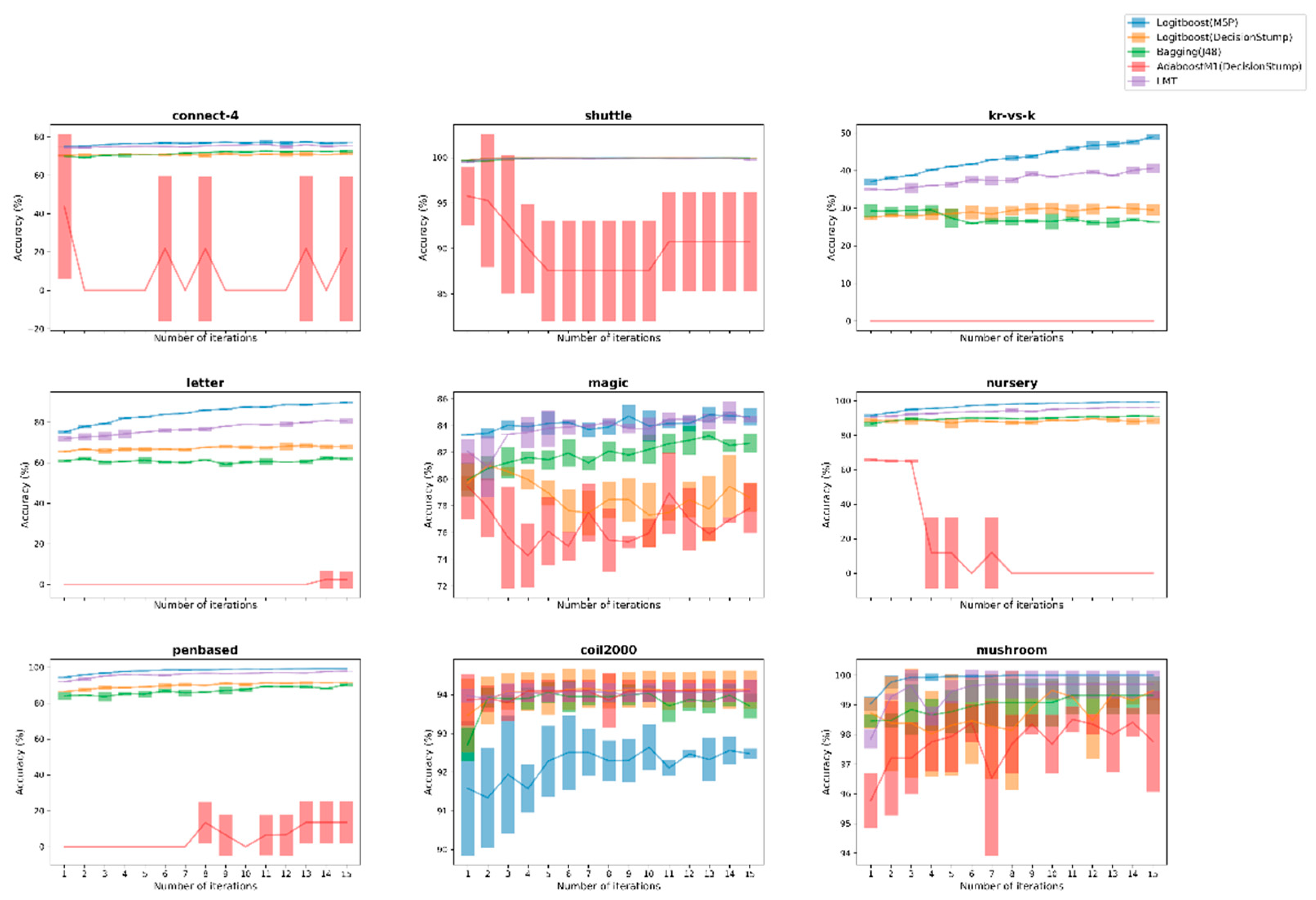
Figure 3.
Comparison of the proposed Logitboost(M5P) against 4 ensemble learners over the 9 larger datasets between both binary and multi-class ones for UncS(LConf) with R = 5%.
Figure 3.
Comparison of the proposed Logitboost(M5P) against 4 ensemble learners over the 9 larger datasets between both binary and multi-class ones for UncS(LConf) with R = 5%.
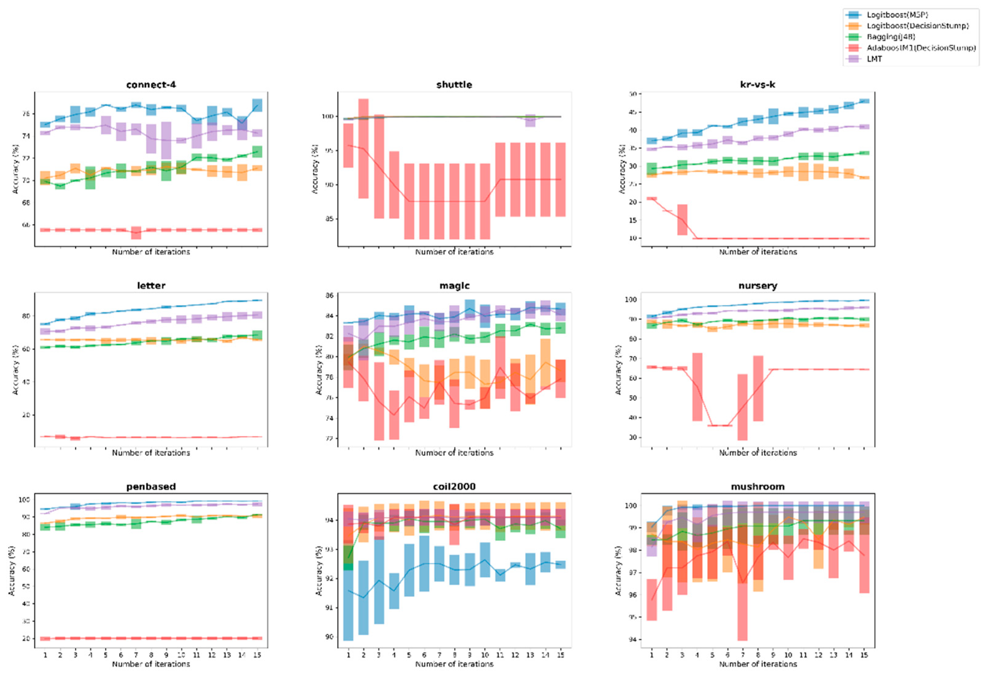
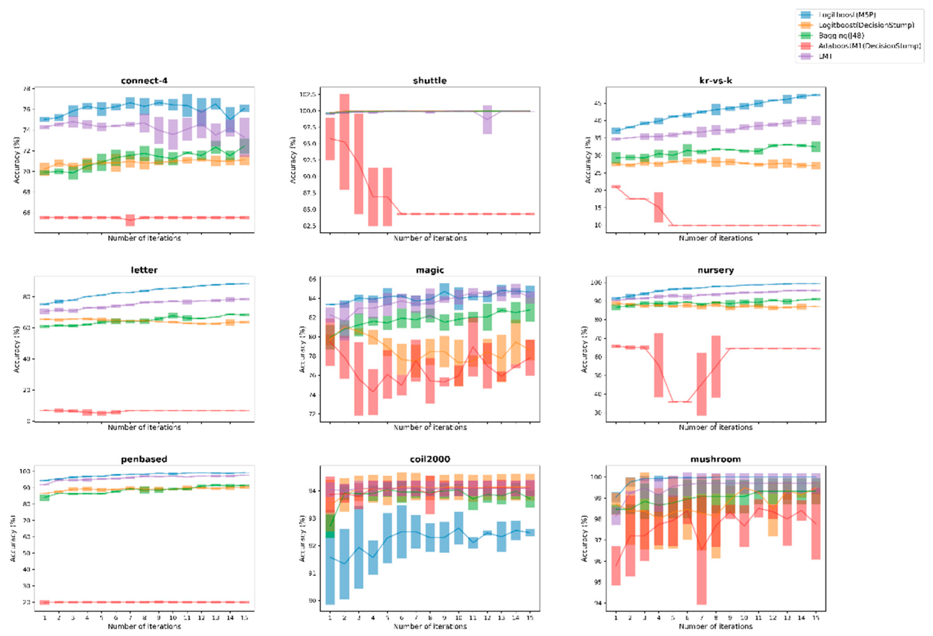
Figure 4.
Comparison of the proposed Logitboost(M5P) against 4 ensemble learners over the 9 larger datasets between both binary and multi-class ones for UncS(SMar) with R = 5%.
Figure 4.
Comparison of the proposed Logitboost(M5P) against 4 ensemble learners over the 9 larger datasets between both binary and multi-class ones for UncS(SMar) with R = 5%.

Table 1.
Formulation of the examined binary class datasets.
| Dataset | n | # of Classes | N | Categorical/Numerical Features | Majority/Minority Class |
|---|---|---|---|---|---|
| appendicitis | 106 | 2 | 7 | 0/7 | 80.189/19.811% |
| banana | 5300 | 2 | 2 | 0/2 | 55.17/44.83% |
| bands | 365 | 2 | 19 | 0/19 | 63.014/36.986% |
| breast-cancer | 286 | 2 | 9 | 9/0 | 70.28/29.72% |
| breast-w | 699 | 2 | 9 | 0/9 | 65.522/34.478% |
| breast | 277 | 2 | 9 | 9/0 | 70.758/29.242% |
| bupa | 345 | 2 | 6 | 0/6 | 57.971/42.029% |
| chess | 3196 | 2 | 36 | 36/0 | 52.222/47.778% |
| coil2000 | 9822 | 2 | 85 | 0/85 | 94.034/5.966% |
| colic | 368 | 2 | 22 | 15/7 | 63.043/36.957% |
| colic.orig | 368 | 2 | 27 | 20/7 | 66.304/33.696% |
| credit-a | 690 | 2 | 15 | 9/6 | 55.507/44.493% |
| credit-g | 1000 | 2 | 20 | 13/7 | 70.0/30.0% |
| crx | 653 | 2 | 15 | 9/6 | 54.671/45.329% |
| diabetes | 768 | 2 | 8 | 0/8 | 65.104/34.896% |
| german | 1000 | 2 | 20 | 13/7 | 70.0/30.0% |
| haberman | 306 | 2 | 3 | 0/3 | 73.529/26.471% |
| heart-statlog | 270 | 2 | 13 | 0/13 | 55.556/44.444% |
| heart | 270 | 2 | 13 | 0/13 | 55.556/44.444% |
| hepatitis | 155 | 2 | 19 | 13/6 | 79.355/20.645% |
| housevotes | 232 | 2 | 16 | 16/0 | 53.448/46.552% |
| ionosphere | 351 | 2 | 34 | 0/34 | 64.103/35.897% |
| kr-vs-kp | 3196 | 2 | 36 | 36/0 | 52.222/47.778% |
| labor | 57 | 2 | 16 | 8/8 | 64.912/35.088% |
| magic | 19,020 | 2 | 10 | 0/10 | 64.837/35.163% |
| mammographic | 830 | 2 | 5 | 0/5 | 51.446/48.554% |
| monk-2 | 432 | 2 | 6 | 0/6 | 52.778/47.222% |
| mushroom | 8124 | 2 | 22 | 22/0 | 51.797/48.203% |
| phoneme | 5404 | 2 | 5 | 0/5 | 70.651/29.349% |
| pima | 768 | 2 | 8 | 0/8 | 65.104/34.896% |
| ring | 7400 | 2 | 20 | 0/20 | 50.486/49.514% |
| saheart | 462 | 2 | 9 | 1/8 | 65.368/34.632% |
| sick | 3772 | 2 | 29 | 22/7 | 93.876/6.124% |
| sonar | 208 | 2 | 60 | 0/60 | 53.365/46.635% |
| spambase | 4597 | 2 | 57 | 0/57 | 60.583/39.417% |
| spectfheart | 267 | 2 | 44 | 0/44 | 79.401/20.599% |
| tic-tac-toe | 958 | 2 | 9 | 9/0 | 65.344/34.656% |
| titanic | 2201 | 2 | 3 | 0/3 | 67.697/32.303% |
| twonorm | 7400 | 2 | 20 | 0/20 | 50.041/49.959% |
| vote | 435 | 2 | 16 | 16/0 | 61.379/38.621% |
| wdbc | 569 | 2 | 30 | 0/30 | 62.742/37.258% |
| wisconsin | 683 | 2 | 9 | 0/9 | 65.007/34.993% |
Table 2.
Formulation of the examined multi-class datasets.
| Dataset | n | # of Classes | N | Categorical/Numerical Features | Majority /Minority Class |
|---|---|---|---|---|---|
| abalone | 4174 | 28 | 8 | 1/7 | 16.507/0.048% |
| anneal | 898 | 6 | 38 | 32/6 | 76.169/0.891% |
| anneal.orig | 898 | 6 | 38 | 32/6 | 76.169/0.891% |
| audiology | 226 | 24 | 69 | 69/0 | 25.221/0.884% |
| automobile | 159 | 6 | 25 | 10/15 | 30.189/10.063% |
| autos | 205 | 7 | 25 | 10/15 | 32.683/1.463% |
| balance-scale | 625 | 3 | 4 | 0/4 | 46.08/53.92% |
| balance | 625 | 3 | 4 | 0/4 | 46.08/53.92% |
| car | 1728 | 4 | 6 | 6/0 | 70.023/7.755% |
| cleveland | 297 | 5 | 13 | 0/13 | 53.872/16.162% |
| connect-4 | 67,557 | 3 | 42 | 42/0 | 65.83/34.17% |
| dermatology | 358 | 6 | 34 | 0/34 | 31.006/18.995% |
| ecoli | 336 | 8 | 7 | 0/7 | 42.56/1.19% |
| flare | 1066 | 6 | 11 | 11/0 | 31.051/12.946% |
| glass | 214 | 7 | 9 | 0/9 | 35.514/4.206% |
| hayes-roth | 160 | 3 | 4 | 0/4 | 40.625/59.375% |
| heart-c | 303 | 5 | 13 | 7/6 | 54.455/0.0% |
| heart-h | 294 | 5 | 13 | 7/6 | 63.946/0.0% |
| hypothyroid | 3772 | 4 | 29 | 22/7 | 92.285/2.572% |
| iris | 150 | 3 | 4 | 0/4 | 33.333/66.666% |
| kr-vs-kp | 28,056 | 18 | 6 | 6/0 | 16.228/0.374% |
| led7digit | 500 | 10 | 7 | 0/7 | 11.4/16.4% |
| letter | 20,000 | 26 | 16 | 0/16 | 4.065/7.34% |
| lymph | 148 | 4 | 18 | 15/3 | 54.73/4.054% |
| lymphography | 148 | 4 | 18 | 15/3 | 54.73/4.054% |
| marketing | 6876 | 9 | 13 | 0/13 | 18.252/15.008% |
| movement_libras | 360 | 15 | 90 | 0/90 | 6.667/13.334% |
| newthyroid | 215 | 3 | 5 | 0/5 | 69.767/30.232% |
| nursery | 12,960 | 5 | 8 | 8/0 | 33.333/2.546% |
| optdigits | 5620 | 10 | 64 | 0/64 | 10.178/19.716% |
| page-blocks | 5472 | 5 | 10 | 0/10 | 89.784/2.102% |
| penbased | 10,992 | 10 | 16 | 0/16 | 10.408/19.196% |
| post-operative | 87 | 3 | 8 | 8/0 | 71.264/28.735% |
| primary-tumor | 339 | 22 | 17 | 17/0 | 24.779/0.295% |
| satimage | 6435 | 7 | 36 | 0/36 | 23.823/9.728% |
| segment | 2310 | 7 | 19 | 0/19 | 14.286/28.572% |
| shuttle | 57,999 | 7 | 9 | 0/9 | 78.598/0.039% |
| soybean | 683 | 19 | 35 | 35/0 | 13.47/3.221% |
| tae | 151 | 3 | 5 | 0/5 | 34.437/65.563% |
| texture | 5500 | 11 | 40 | 0/40 | 9.091/18.182% |
| thyroid | 7200 | 3 | 21 | 0/21 | 92.583/7.417% |
| vehicle | 846 | 4 | 18 | 0/18 | 25.768/48.581% |
Table 3.
Classification accuracy of the Logitboost(M5P) against the selected simple base learners for binary datasets under UncS(Ent) strategy with R = 5%.
Table 3.
Classification accuracy of the Logitboost(M5P) against the selected simple base learners for binary datasets under UncS(Ent) strategy with R = 5%.
| Datasets | Logitboost (M5P) | 1NN | 3NN | 5-NN | J48 | JRip | Random Tree | NB |
|---|---|---|---|---|---|---|---|---|
| appendicitis | 75.84 | 80.56 | 82.07 | 81.13 | 80.16 | 80.47 | 79.59 | 78.63 |
| banana | 87.06 | 84.86 | 84.69 | 86.64 | 71.54 | 78.87 | 83.30 | 83.08 |
| bands | 58.63 | 46.76 | 40.08 | 39.00 | 50.96 | 39.09 | 42.56 | 46.76 |
| breast-cancer | 66.08 | 72.15 | 70.63 | 69.82 | 70.15 | 70.40 | 67.03 | 67.84 |
| breast-w | 95.66 | 88.75 | 93.66 | 94.90 | 87.94 | 86.55 | 88.08 | 90.10 |
| breast | 69.92 | 72.31 | 71.71 | 72.68 | 69.67 | 69.18 | 69.32 | 69.47 |
| bupa | 61.26 | 48.21 | 44.25 | 44.06 | 49.37 | 43.29 | 52.17 | 52.24 |
| chess | 97.68 | 80.44 | 79.81 | 79.62 | 92.98 | 88.64 | 82.64 | 89.66 |
| coil2000 | 92.63 | 92.49 | 93.71 | 93.99 | 94.03 | 94.02 | 91.54 | 92.73 |
| colic.ORIG | 66.39 | 64.77 | 66.75 | 65.67 | 66.13 | 69.85 | 67.21 | 67.82 |
| colic | 78.54 | 72.47 | 66.56 | 69.84 | 63.05 | 64.95 | 62.05 | 68.51 |
| credit-a | 81.74 | 67.83 | 63.86 | 67.54 | 84.30 | 70.58 | 64.30 | 72.21 |
| credit-g | 69.47 | 69.43 | 70.53 | 70.13 | 67.27 | 69.87 | 67.27 | 68.87 |
| crx | 79.48 | 68.30 | 62.62 | 67.59 | 86.17 | 70.48 | 60.59 | 70.18 |
| diabetes | 71.22 | 67.62 | 65.93 | 65.67 | 68.32 | 66.62 | 68.84 | 68.89 |
| german | 69.23 | 69.34 | 70.57 | 70.47 | 69.97 | 69.83 | 67.14 | 68.73 |
| haberman | 72.22 | 43.14 | 32.57 | 31.92 | 42.16 | 31.70 | 40.74 | 48.22 |
| heart-c | 77.23 | 68.32 | 66.12 | 70.85 | 64.25 | 58.64 | 60.62 | 65.49 |
| heart-h | 73.36 | 73.47 | 74.94 | 69.05 | 65.99 | 67.12 | 66.78 | 69.09 |
| heart-statlog | 75.06 | 72.96 | 63.21 | 63.95 | 70.25 | 59.26 | 65.68 | 66.67 |
| heart | 74.81 | 72.35 | 61.98 | 65.93 | 63.95 | 62.35 | 63.58 | 66.91 |
| hepatitis | 78.28 | 59.84 | 61.76 | 64.37 | 54.01 | 46.23 | 44.93 | 56.48 |
| housevotes | 96.11 | 90.51 | 89.50 | 90.80 | 88.49 | 93.81 | 87.04 | 92.32 |
| ionosphere | 84.52 | 79.68 | 73.03 | 69.80 | 65.62 | 53.37 | 59.45 | 65.78 |
| kr-vs-kp | 97.48 | 80.09 | 80.03 | 80.04 | 90.93 | 91.28 | 83.07 | 90.61 |
| labor | 76.02 | 53.80 | 74.27 | 49.71 | 42.69 | 44.44 | 52.05 | 57.50 |
| magic | 84.53 | 76.82 | 74.21 | 77.20 | 80.64 | 79.67 | 79.44 | 81.21 |
| mammographic | 81.65 | 65.46 | 63.38 | 61.21 | 66.75 | 64.58 | 70.20 | 72.14 |
| monk-2 | 98.30 | 73.53 | 71.60 | 70.14 | 97.22 | 95.52 | 81.40 | 91.74 |
| mushroom | 99.77 | 99.98 | 99.98 | 99.98 | 98.52 | 99.20 | 99.10 | 99.36 |
| phoneme | 81.49 | 78.23 | 74.17 | 76.17 | 73.30 | 72.48 | 76.49 | 76.82 |
| pima | 71.09 | 65.45 | 66.71 | 65.58 | 66.84 | 65.32 | 69.70 | 68.71 |
| ring | 89.20 | 76.50 | 73.08 | 69.57 | 81.28 | 65.74 | 79.53 | 78.16 |
| saheart | 62.63 | 63.35 | 65.44 | 66.09 | 64.86 | 66.02 | 63.28 | 63.97 |
| sick | 98.37 | 94.72 | 95.23 | 95.09 | 95.64 | 96.34 | 94.87 | 96.53 |
| sonar | 65.71 | 55.77 | 49.35 | 48.56 | 56.89 | 48.22 | 56.07 | 56.67 |
| spambase | 90.80 | 75.26 | 71.53 | 71.03 | 85.87 | 84.48 | 79.52 | 84.93 |
| spectfheart | 73.03 | 47.44 | 49.56 | 44.57 | 56.05 | 45.44 | 49.94 | 56.14 |
| tic-tac-toe | 83.61 | 76.23 | 71.99 | 70.84 | 65.62 | 68.23 | 68.09 | 73.31 |
| titanic | 77.92 | 77.62 | 77.09 | 77.16 | 73.80 | 73.30 | 77.34 | 76.19 |
| twonorm | 96.23 | 91.39 | 91.25 | 93.58 | 78.45 | 79.34 | 77.03 | 84.20 |
| vote | 95.10 | 92.03 | 93.33 | 93.87 | 93.03 | 89.35 | 88.58 | 91.01 |
| wdbc | 95.66 | 88.69 | 88.70 | 91.04 | 84.29 | 81.43 | 86.18 | 87.76 |
| wisconsin | 96.10 | 87.85 | 95.17 | 95.90 | 87.26 | 87.94 | 88.96 | 91.00 |
Bold: the best value per dataset (row) achieved by all the included algorithms (columns).
Table 4.
Classification accuracy of the Logitboost(M5P) against the selected simple base learners for multi-class datasets under UncS(Ent) strategy with R = 5%.
Table 4.
Classification accuracy of the Logitboost(M5P) against the selected simple base learners for multi-class datasets under UncS(Ent) strategy with R = 5%.
| Datasets | Logitboost (M5P) | 1NN | 3NN | 5NN | J48 | JRip | Random Tree | NB |
|---|---|---|---|---|---|---|---|---|
| abalone | 22.03 | 17.42 | 17.38 | 21.92 | 20.84 | 11.48 | 17.25 | 16.92 |
| anneal.ORIG | 84.71 | 83.93 | 84.52 | 83.48 | 75.54 | 73.64 | 81.99 | 80.12 |
| anneal | 92.80 | 75.24 | 82.14 | 86.23 | 85.86 | 84.59 | 86.37 | 87.92 |
| audiology | 48.84 | 34.93 | 39.56 | 34.67 | 55.76 | 26.72 | 32.02 | 35.86 |
| automobile | 47.59 | 34.38 | 33.54 | 26.21 | 36.27 | 17.82 | 39.83 | 35.08 |
| autos | 43.74 | 28.61 | 21.95 | 18.84 | 37.88 | 11.21 | 35.93 | 30.29 |
| balance-scale | 85.60 | 73.39 | 77.60 | 79.78 | 64.37 | 61.55 | 67.68 | 71.61 |
| balance | 87.62 | 71.57 | 77.39 | 79.68 | 65.23 | 64.47 | 67.89 | 73.33 |
| car | 89.91 | 79.24 | 80.71 | 80.34 | 71.74 | 71.28 | 73.53 | 78.24 |
| cleveland | 50.84 | 55.44 | 55.56 | 55.22 | 52.97 | 53.20 | 52.19 | 52.08 |
| connect-4 | 76.32 | 70.65 | 72.57 | 73.07 | 71.36 | 69.24 | 64.40 | 69.99 |
| dermatology | 93.95 | 80.43 | 90.79 | 91.72 | 66.88 | 53.79 | 63.98 | 70.57 |
| ecoli | 73.12 | 58.83 | 69.35 | 69.44 | 62.00 | 52.08 | 57.84 | 61.01 |
| flare | 72.95 | 66.57 | 67.10 | 63.44 | 61.92 | 67.86 | 64.20 | 68.33 |
| glass | 51.87 | 39.38 | 38.13 | 40.96 | 36.93 | 36.47 | 41.00 | 43.11 |
| hayes-roth | 51.89 | 44.54 | 43.13 | 40.61 | 41.69 | 41.88 | 49.64 | 47.80 |
| hypothyroid | 99.43 | 91.25 | 92.82 | 92.54 | 97.92 | 97.68 | 94.29 | 97.13 |
| iris | 83.78 | 85.33 | 85.11 | 83.56 | 64.22 | 43.78 | 71.56 | 66.37 |
| kr-vs-kp | 47.88 | 39.74 | 40.16 | 39.96 | 30.66 | 15.50 | 28.88 | 30.75 |
| led7digit | 56.00 | 61.34 | 51.48 | 47.53 | 41.33 | 25.39 | 47.40 | 42.93 |
| letter | 88.49 | 79.07 | 75.23 | 73.98 | 62.63 | 58.19 | 56.75 | 67.81 |
| lymph | 74.77 | 65.51 | 69.82 | 69.57 | 55.90 | 55.64 | 61.49 | 63.96 |
| lymphography | 70.72 | 66.41 | 72.29 | 69.45 | 59.46 | 57.19 | 61.71 | 63.21 |
| marketing | 26.88 | 26.87 | 25.16 | 26.84 | 26.52 | 23.27 | 25.56 | 25.24 |
| movement_libras | 38.15 | 39.54 | 33.98 | 32.22 | 24.44 | 10.37 | 20.56 | 23.02 |
| newthyroid | 83.84 | 81.87 | 83.41 | 85.86 | 76.87 | 71.48 | 79.86 | 78.39 |
| nursery | 99.57 | 85.59 | 87.92 | 86.25 | 88.12 | 82.81 | 83.16 | 88.51 |
| optdigits | 97.16 | 92.89 | 96.52 | 97.11 | 72.25 | 68.79 | 61.92 | 75.96 |
| page-blocks | 96.52 | 93.07 | 94.67 | 94.54 | 94.35 | 94.24 | 93.75 | 94.84 |
| penbased | 99.05 | 95.60 | 98.39 | 98.38 | 86.70 | 82.17 | 82.27 | 87.83 |
| post-operative | 68.20 | 68.58 | 70.88 | 71.26 | 71.26 | 71.26 | 67.43 | 68.97 |
| primary-tumor | 30.29 | 29.99 | 29.79 | 27.63 | 24.29 | 25.66 | 28.12 | 28.02 |
| satimage | 87.38 | 68.38 | 85.92 | 85.39 | 70.01 | 64.72 | 61.53 | 71.21 |
| segment | 94.49 | 86.81 | 88.74 | 86.58 | 85.11 | 77.52 | 78.14 | 83.38 |
| shuttle | 99.98 | 99.72 | 99.83 | 99.79 | 99.79 | 99.81 | 99.69 | 99.82 |
| soybean | 76.53 | 78.67 | 66.96 | 57.30 | 46.18 | 46.91 | 47.28 | 56.91 |
| tae | 45.26 | 38.41 | 34.24 | 37.95 | 36.41 | 33.80 | 40.59 | 39.88 |
| texture | 98.21 | 90.79 | 94.53 | 95.28 | 80.82 | 75.14 | 70.76 | 81.37 |
| thyroid | 99.60 | 62.75 | 81.70 | 87.46 | 98.92 | 98.60 | 93.14 | 97.11 |
| vehicle | 70.57 | 45.90 | 40.70 | 45.11 | 45.63 | 39.95 | 46.22 | 52.25 |
| vowel | 49.43 | 26.33 | 14.04 | 15.79 | 35.35 | 18.72 | 26.73 | 31.63 |
| waveform-5000 | 82.65 | 63.79 | 68.40 | 75.93 | 68.51 | 62.35 | 59.89 | 68.30 |
| wine | 96.63 | 77.70 | 84.62 | 86.15 | 60.07 | 46.28 | 55.10 | 66.00 |
| winequalityRed | 51.53 | 33.25 | 47.07 | 47.59 | 37.92 | 35.81 | 31.08 | 39.48 |
| winequalityWhite | 49.16 | 37.31 | 45.12 | 45.15 | 41.00 | 35.08 | 34.18 | 39.47 |
| yeast | 51.84 | 37.71 | 39.92 | 46.45 | 36.07 | 30.21 | 33.76 | 38.61 |
| zoo | 26.43 | 75.55 | 81.55 | 68.26 | 60.24 | 41.24 | 50.69 | 39.45 |
Bold: the best value per dataset (row) achieved by all the included algorithms (columns).
Table 5.
Classification accuracy of the Logitboost(M5P) against the selected ensemble base learners for binary datasets under UncS(Ent) strategy with R = 5%.
Table 5.
Classification accuracy of the Logitboost(M5P) against the selected ensemble base learners for binary datasets under UncS(Ent) strategy with R = 5%.
| Datasets | Logitboost (M5P) | Logitboost (DStump) | Bagging (J48) | Ada (DStump) | LMT |
|---|---|---|---|---|---|
| banana | 87.06 | 84.48 | 83.35 | 59.25 | 71.91 |
| bands | 58.63 | 49.32 | 47.21 | 55.14 | 57.90 |
| breast-w | 95.66 | 91.28 | 90.32 | 92.61 | 95.52 |
| chess | 97.68 | 90.00 | 95.78 | 84.38 | 98.14 |
| coil2000 | 92.63 | 92.30 | 93.49 | 94.03 | 94.03 |
| credit-a | 81.74 | 72.75 | 81.06 | 84.88 | 79.76 |
| credit-g | 69.47 | 68.53 | 69.53 | 70.63 | 69.80 |
| german | 69.23 | 68.37 | 68.73 | 70.47 | 69.47 |
| heart-statlog | 75.06 | 69.14 | 60.25 | 70.49 | 70.25 |
| housevotes | 96.11 | 91.82 | 94.67 | 94.82 | 95.25 |
| ionosphere | 84.52 | 69.92 | 62.20 | 74.45 | 83.86 |
| kr-vs-kp | 97.48 | 90.39 | 95.58 | 86.57 | 98.04 |
| magic | 84.53 | 81.73 | 82.88 | 77.14 | 84.33 |
| mammographic | 81.65 | 74.66 | 79.52 | 79.92 | 80.97 |
| monk-2 | 98.30 | 90.48 | 97.22 | 95.76 | 93.98 |
| mushroom | 99.77 | 99.41 | 99.36 | 97.58 | 99.60 |
| phoneme | 81.49 | 78.26 | 80.47 | 72.25 | 79.42 |
| pima | 71.09 | 69.84 | 69.01 | 70.66 | 73.13 |
| ring | 89.20 | 82.30 | 87.62 | 49.51 | 83.88 |
| sick | 98.37 | 96.59 | 98.12 | 97.52 | 98.34 |
| sonar | 65.71 | 59.48 | 52.57 | 60.73 | 60.28 |
| spambase | 90.80 | 85.08 | 89.66 | 83.76 | 92.70 |
| spectfheart | 73.03 | 59.70 | 49.44 | 69.91 | 72.28 |
| tic-tac-toe | 83.61 | 75.01 | 67.40 | 69.07 | 72.41 |
| titanic | 77.92 | 77.15 | 78.27 | 77.66 | 77.56 |
| twonorm | 96.23 | 85.82 | 86.36 | 84.81 | 97.79 |
| vote | 95.10 | 91.56 | 88.35 | 92.72 | 85.06 |
| wdbc | 95.66 | 89.87 | 85.76 | 94.38 | 97.01 |
| wisconsin | 96.10 | 92.02 | 92.97 | 92.97 | 96.58 |
Bold: the best value per dataset (row) achieved by all the included algorithms (columns).
Table 6.
Classification accuracy of the Logitboost(M5P) against the selected ensemble base learners for multi-class datasets under UncS(Ent) strategy with R = 5%.
Table 6.
Classification accuracy of the Logitboost(M5P) against the selected ensemble base learners for multi-class datasets under UncS(Ent) strategy with R = 5%.
| Datasets | Logitboost (M5P) | Logitboost (DStump) | Bagging (J48) | Ada (DStump) | LMT |
|---|---|---|---|---|---|
| abalone | 22.03 | 18.73 | 19.94 | 16.73 | 22.73 |
| anneal.ORIG | 84.71 | 82.27 | 76.80 | 75.57 | 82.75 |
| anneal | 92.80 | 89.03 | 85.15 | 77.02 | 92.28 |
| audiology | 48.84 | 38.91 | 49.10 | 33.90 | 54.27 |
| automobile | 47.59 | 40.83 | 37.11 | 23.48 | 43.40 |
| balance-scale | 85.60 | 74.96 | 71.84 | 49.81 | 84.00 |
| balance | 87.62 | 76.28 | 66.98 | 55.90 | 85.49 |
| car | 89.91 | 80.56 | 78.34 | 70.79 | 87.29 |
| cleveland | 50.84 | 51.70 | 53.87 | 53.98 | 53.20 |
| connect-4 | 76.32 | 70.24 | 72.67 | 65.83 | 73.44 |
| dermatology | 93.95 | 76.17 | 86.31 | 48.70 | 93.02 |
| ecoli | 73.12 | 63.99 | 68.15 | 62.00 | 71.73 |
| flare | 72.95 | 68.49 | 68.73 | 53.47 | 69.20 |
| glass | 51.87 | 45.33 | 40.80 | 38.95 | 42.39 |
| hayes-roth | 51.89 | 49.78 | 45.24 | 48.12 | 46.27 |
| hypothyroid | 99.43 | 96.95 | 99.51 | 93.83 | 99.11 |
| iris | 83.78 | 73.90 | 70.22 | 80.00 | 73.56 |
| kr-vs-kp | 47.88 | 35.84 | 33.56 | 10.04 | 40.32 |
| led7digit | 56.00 | 48.78 | 47.00 | 14.94 | 57.00 |
| letter | 88.49 | 71.02 | 68.15 | 6.91 | 78.27 |
| marketing | 26.88 | 25.89 | 26.59 | 18.64 | 29.35 |
| movement_libras | 38.15 | 27.24 | 24.35 | 10.93 | 40.37 |
| newthyroid | 83.84 | 80.70 | 78.79 | 81.26 | 89.15 |
| nursery | 99.57 | 90.41 | 90.74 | 64.54 | 95.40 |
| optdigits | 97.16 | 78.35 | 81.60 | 18.74 | 95.07 |
| page-blocks | 96.52 | 95.04 | 96.06 | 92.60 | 96.64 |
| penbased | 99.05 | 89.72 | 91.95 | 20.52 | 97.45 |
| primary-tumor | 30.29 | 28.81 | 24.39 | 25.86 | 24.98 |
| satimage | 87.38 | 73.37 | 81.66 | 33.63 | 83.01 |
| segment | 94.49 | 85.34 | 89.25 | 28.51 | 91.53 |
| shuttle | 99.98 | 99.83 | 99.96 | 84.23 | 99.92 |
| soybean | 76.53 | 60.24 | 43.88 | 13.47 | 74.73 |
| tae | 45.26 | 41.91 | 35.76 | 35.74 | 37.08 |
| texture | 98.21 | 83.45 | 84.93 | 16.08 | 99.59 |
| thyroid | 99.60 | 96.62 | 99.36 | 96.87 | 99.54 |
| vehicle | 70.57 | 56.34 | 52.44 | 26.04 | 68.36 |
| vowel | 49.43 | 35.93 | 39.66 | 14.14 | 50.10 |
| waveform-5000 | 82.65 | 70.28 | 75.00 | 55.37 | 86.33 |
| wine | 96.63 | 72.58 | 64.28 | 69.14 | 80.56 |
| winequalityRed | 51.53 | 40.70 | 46.32 | 42.21 | 50.49 |
| winequalityWhite | 49.16 | 40.94 | 47.39 | 31.19 | 49.24 |
| yeast | 51.84 | 41.40 | 47.15 | 21.29 | 54.09 |
Bold: the best value per dataset (row) achieved by all the included algorithms (columns).
Table 7.
Number of best achieved performances over the examined datasets per base learner for the included query strategies and R-based experiments the comparison of simple learners.
Table 7.
Number of best achieved performances over the examined datasets per base learner for the included query strategies and R-based experiments the comparison of simple learners.
| QS (metric) | Logitboost (M5P) | 1NN | 3NN | 5NN | J48 | Random Tree | JRip | NB |
|---|---|---|---|---|---|---|---|---|
| Binary Datasets | ||||||||
| R = 5% | ||||||||
| UncS(Ent) | 32 | 2 | 4 | 3 | 3 | 0 | 1 | 0 |
| UncS(LConf) | 33 | 2 | 4 | 3 | 2 | 0 | 1 | 0 |
| UncS(SMar) | 33 | 2 | 4 | 3 | 2 | 1 | 0 | 0 |
| R = 10% | ||||||||
| UncS(Ent) | 30 | 0 | 3 | 7 | 2 | 0 | 3 | 0 |
| UncS(LConf) | 30 | 0 | 3 | 7 | 2 | 0 | 3 | 0 |
| UncS(SMar) | 31 | 0 | 3 | 7 | 3 | 1 | 0 | 0 |
| R = 15% | ||||||||
| UncS(Ent) | 26 | 0 | 6 | 8 | 3 | 0 | 2 | 0 |
| UncS(LConf) | 26 | 0 | 6 | 8 | 3 | 0 | 2 | 0 |
| UncS(SMar) | 27 | 0 | 6 | 9 | 3 | 0 | 0 | 0 |
| R = 20% | ||||||||
| UncS(Ent) | 23 | 2 | 6 | 4 | 5 | 1 | 4 | 0 |
| UncS(LConf) | 23 | 2 | 6 | 4 | 5 | 1 | 4 | 0 |
| UncS(SMar) | 26 | 2 | 6 | 5 | 5 | 1 | 0 | 0 |
| Multi-Class Datasets | ||||||||
| R = 5% | ||||||||
| UncS(Ent) | 37 | 4 | 3 | 2 | 2 | 0 | 1 | 0 |
| UncS(LConf) | 38 | 3 | 3 | 1 | 2 | 1 | 1 | 0 |
| UncS(SMar) | 37 | 3 | 4 | 1 | 2 | 1 | - | 0 |
| R = 10% | ||||||||
| UncS(Ent) | 36 | 2 | 4 | 5 | 0 | 0 | 0 | 0 |
| UncS(LConf) | 38 | 1 | 6 | 2 | 0 | 0 | 0 | 0 |
| UncS(SMar) | 38 | 0 | 7 | 1 | 1 | 0 | - | 0 |
| R = 15% | ||||||||
| UncS(Ent) | 34 | 5 | 3 | 4 | 1 | 0 | 1 | 0 |
| UncS(LConf) | 35 | 3 | 6 | 2 | 1 | 0 | 1 | 0 |
| UncS(SMar) | 35 | 3 | 3 | 5 | 1 | 0 | - | 0 |
| R = 20% | ||||||||
| UncS(Ent) | 35 | 1 | 3 | 3 | 4 | 1 | 0 | 0 |
| UncS(LConf) | 35 | 1 | 4 | 2 | 5 | 1 | 0 | 0 |
| UncS(SMar) | 36 | 2 | 2 | 2 | 4 | 1 | - | 0 |
| Total | 774 | 40 | 105 | 98 | 61 | 10 | 24 | 0 |
Table 8.
The number of best achieved performance over the examined datasets per base learner for the included query strategies and R-based experiments compared to ensemble learners.
Table 8.
The number of best achieved performance over the examined datasets per base learner for the included query strategies and R-based experiments compared to ensemble learners.
| QS (metric) | Logitboost (M5P) | Logitboost (DStump) | Bagging (J48) | Ada (DStump) | LMT |
|---|---|---|---|---|---|
| Binary Datasets | |||||
| R = 5% | |||||
| UncS(Ent) | 17 | 0 | 1 | 4 | 8 |
| UncS(LConf) | 16 | 0 | 1 | 2 | 10 |
| UncS(SMar) | 16 | 0 | 1 | 2 | 10 |
| R = 10% | |||||
| UncS(Ent) | 16 | 0 | 3 | 3 | 9 |
| UncS(LConf) | 18 | 0 | 3 | 3 | 7 |
| UncS(SMar) | 18 | 0 | 2 | 4 | 7 |
| R = 15% | |||||
| UncS(Ent) | 14 | 0 | 4 | 3 | 9 |
| UncS(LConf) | 12 | 0 | 4 | 4 | 11 |
| UncS(SMar) | 12 | 0 | 4 | 3 | 12 |
| R = 20% | |||||
| UncS(Ent) | 10 | 1 | 1 | 3 | 14 |
| UncS(LConf) | 10 | 1 | 1 | 3 | 14 |
| UncS(SMar) | 12 | 0 | 1 | 3 | 14 |
| Multi-Class Datasets | |||||
| R = 5% | |||||
| UncS(Ent) | 28 | 1 | 0 | 1 | 12 |
| UncS(LConf) | 27 | 1 | 0 | 1 | 13 |
| UncS(SMar) | 27 | 1 | 0 | 0 | 14 |
| R = 10% | |||||
| UncS(Ent) | 28 | 5 | 0 | 0 | 9 |
| UncS(LConf) | 28 | 3 | 0 | 0 | 11 |
| UncS(SMar) | 26 | 2 | 0 | 0 | 14 |
| R = 15% | |||||
| UncS(Ent) | 29 | 1 | 0 | 1 | 12 |
| UncS(LConf) | 26 | 1 | 0 | 0 | 15 |
| UncS(SMar) | 27 | 2 | 0 | 0 | 13 |
| R = 20% | |||||
| UncS(Ent) | 28 | 1 | 0 | 0 | 13 |
| UncS(LConf) | 26 | 4 | 0 | 0 | 12 |
| UncS(SMar) | 28 | 3 | 0 | 0 | 11 |
| Total | 499 | 51 | 2 | 40 | 274 |
Table 9.
Freidman ranking scores of the second experimental setup.
| Active Learning Approaches | Binary | Multiclass | Average | ||||||
|---|---|---|---|---|---|---|---|---|---|
| R(%) | 5% | 10% | 15% | 20% | 5% | 10% | 15% | 20% | |
| UncS(Logitboost(M5P)) | 2.138 | 2.511 | 2.477 | 3.040 | 2.270 | 1.948 | 1.921 | 2.270 | 2.322 |
| UncS(LMT) | 3.787 | 3.000 | 2.563 | 2.328 | 3.321 | 2.813 | 2.528 | 3.321 | 2.958 |
| RS(LMT) | 4.437 | 4.230 | 4.540 | 3.632 | 3.468 | 3.603 | 3.659 | 3.468 | 3.880 |
| RS(Logitboost(M5P)) | 4.851 | 5.109 | 4.839 | 4.983 | 3.079 | 3.016 | 3.452 | 3.079 | 4.051 |
| RS(Ada(DStump)) | 5.437 | 6.132 | 6.943 | 6.977 | 8.238 | 8.889 | 9.246 | 8.238 | 7.513 |
| RS(Bagging(J48)) | 5.833 | 6.672 | 6.483 | 6.316 | 5.921 | 6.298 | 6.286 | 5.921 | 6.216 |
| UncS(Ada(DStump)) | 6.626 | 5.707 | 5.931 | 6.575 | 9.381 | 9.381 | 8.937 | 9.381 | 7.740 |
| UncS(Bagging(J48)) | 6.339 | 5.282 | 4.695 | 4.908 | 6.560 | 5.583 | 5.440 | 6.560 | 5.671 |
| RS((Logitboost(DStump))) | 7.080 | 7.678 | 7.793 | 8.241 | 5.516 | 6.111 | 6.214 | 5.516 | 6.769 |
| UncS((Logitboost(DStump))) | 8.471 | 8.678 | 8.736 | 8.000 | 7.246 | 7.357 | 7.317 | 7.246 | 7.881 |
Bold: the best value per dataset (row) achieved by all the included algorithms (columns).
Table 10.
Freidman ranking scores for hyperparameter tuning of the Logitboost scheme.
| Active Learning Approaches | Binary | Multiclass | Average | ||||||
|---|---|---|---|---|---|---|---|---|---|
| R(%) | 5% | 10% | 15% | 20% | 5% | 10% | 15% | 20% | |
| Ent(5 iterations) | 3.32 | 3.88 | 3.69 | 3.50 | 3.94 | 3.82 | 3.95 | 3.83 | 3.74 |
| Ent(10 iterations) | 3.38 | 2.86 | 3.09 | 2.93 | 2.47 | 3.07 | 2.89 | 3.39 | 3.01 |
| Ent(15 iterations) | 3.01 | 2.98 | 2.58 | 3.20 | 3.15 | 3.07 | 3.02 | 2.60 | 3.00 |
| Ent(20 iterations) | 2.36 | 2.75 | 2.74 | 2.51 | 2.73 | 2.74 | 2.66 | 2.78 | 2.66 |
| Ent(25 iterations) | 2.93 | 2.53 | 2.90 | 2.85 | 2.71 | 2.29 | 2.48 | 2.40 | 2.64 |
| LConf(5 iterations) | 3.39 | 3.83 | 3.65 | 3.51 | 3.46 | 4.00 | 3.95 | 3.86 | 3.71 |
| LConf(10 iterations) | 3.31 | 2.95 | 3.05 | 3.18 | 2.90 | 2.82 | 2.99 | 2.66 | 2.98 |
| LConf(15 iterations) | 3.02 | 2.93 | 2.94 | 2.94 | 3.20 | 2.88 | 3.20 | 3.59 | 3.09 |
| LConf(20 iterations) | 2.30 | 2.77 | 2.63 | 2.51 | 2.81 | 2.73 | 2.51 | 2.60 | 2.61 |
| LConf(25 iterations) | 2.99 | 2.51 | 2.74 | 2.85 | 2.63 | 2.56 | 2.35 | 2.30 | 2.62 |
| SMar(5 iterations) | 3.35 | 3.78 | 3.65 | 3.47 | 3.83 | 3.99 | 3.82 | 3.89 | 3.72 |
| SMar(10 iterations) | 3.33 | 2.95 | 3.09 | 2.90 | 2.98 | 2.95 | 3.17 | 3.23 | 3.08 |
| SMar(15 iterations) | 3.03 | 2.93 | 2.60 | 3.15 | 2.72 | 2.80 | 2.63 | 2.57 | 2.80 |
| SMar(20 iterations) | 2.30 | 2.80 | 2.73 | 2.49 | 2.78 | 2.83 | 3.07 | 2.76 | 2.72 |
| SMar(25 iterations) | 2.99 | 2.53 | 2.93 | 3.00 | 2.69 | 2.44 | 2.31 | 2.54 | 2.68 |
Bold: the best value per dataset (row) achieved by all the included algorithms (columns).
Publisher’s Note: MDPI stays neutral with regard to jurisdictional claims in published maps and institutional affiliations. |
© 2020 by the authors. Licensee MDPI, Basel, Switzerland. This article is an open access article distributed under the terms and conditions of the Creative Commons Attribution (CC BY) license (http://creativecommons.org/licenses/by/4.0/).
Share and Cite
MDPI and ACS Style
Kazllarof, V.; Karlos, S.; Kotsiantis, S. Investigation of Combining Logitboost(M5P) under Active Learning Classification Tasks. Informatics 2020, 7, 50. https://0-doi-org.brum.beds.ac.uk/10.3390/informatics7040050
AMA Style
Kazllarof V, Karlos S, Kotsiantis S. Investigation of Combining Logitboost(M5P) under Active Learning Classification Tasks. Informatics. 2020; 7(4):50. https://0-doi-org.brum.beds.ac.uk/10.3390/informatics7040050
Chicago/Turabian StyleKazllarof, Vangjel, Stamatis Karlos, and Sotiris Kotsiantis. 2020. "Investigation of Combining Logitboost(M5P) under Active Learning Classification Tasks" Informatics 7, no. 4: 50. https://0-doi-org.brum.beds.ac.uk/10.3390/informatics7040050
Note that from the first issue of 2016, this journal uses article numbers instead of page numbers. See further details here.