Windows PE Malware Detection Using Ensemble Learning
by
 , ,
, ,
Nureni Ayofe Azeez
1 ,
,
Oluwanifise Ebunoluwa Odufuwa
1,
Sanjay Misra
2,3,
Jonathan Oluranti
2 and
Robertas Damaševičius
4,* 1
Department of Computer Sciences, Faculty of Science, University of Lagos, Lagos 100001, Nigeria
2
Center of ICT/ICE Research, CUCRID, Covenant University, Ota 112212, Nigeria
3
Department of Computer Engineering, Atilim University, Ankara 06830, Turkey
4
Department of Applied Informatics, Vytautas Magnus University, 44404 Kaunas, Lithuania
*
Author to whom correspondence should be addressed.
Informatics 2021, 8(1), 10; https://0-doi-org.brum.beds.ac.uk/10.3390/informatics8010010
Submission received: 21 December 2020
/
Revised: 5 February 2021
/
Accepted: 8 February 2021
/
Published: 10 February 2021
(This article belongs to the Special Issue Towards the Next-Generation of Network Monitoring Systems)
Abstract
:In this Internet age, there are increasingly many threats to the security and safety of users daily. One of such threats is malicious software otherwise known as malware (ransomware, Trojans, viruses, etc.). The effect of this threat can lead to loss or malicious replacement of important information (such as bank account details, etc.). Malware creators have been able to bypass traditional methods of malware detection, which can be time-consuming and unreliable for unknown malware. This motivates the need for intelligent ways to detect malware, especially new malware which have not been evaluated or studied before. Machine learning provides an intelligent way to detect malware and comprises two stages: feature extraction and classification. This study suggests an ensemble learning-based method for malware detection. The base stage classification is done by a stacked ensemble of fully-connected and one-dimensional convolutional neural networks (CNNs), whereas the end-stage classification is done by a machine learning algorithm. For a meta-learner, we analyzed and compared 15 machine learning classifiers. For comparison, five machine learning algorithms were used: naïve Bayes, decision tree, random forest, gradient boosting, and AdaBoosting. The results of experiments made on the Windows Portable Executable (PE) malware dataset are presented. The best results were obtained by an ensemble of seven neural networks and the ExtraTrees classifier as a final-stage classifier.
1. Introduction
The popularity of the Internet has been skyrocketing since its invention. A report from the International Telecommunication Union (ITU) indicates that 51.2% of the population of the world, or 3.9 billion people, were using the Internet as of the close of 2018 [1]. The more popular the Internet becomes, the more vulnerable Internet users are because of cybercriminals who employ various methods to attack or damage computers, servers, clients, or computer networks for their financial or political benefit. One of the methods employed by cybercriminals is the use of malicious software, otherwise known as malware, to exploit a system’s vulnerabilities and to affect the user or device. Malware is any software purposely designed to inflict harm to a computer system—a server, a client, or a computer network—for personal benefits. Malware can be classified based on how it multiplies or its particular action. The various types of malware include viruses, worms, Trojan horses, adware, spyware, rootkits, bots, ransomware, etc. [2,3,4].
Malevolent cyberattacks may cause considerable losses, whether they arise from a single person, an organization, or a hostile state. As colluded attacks on computer networks become more common, the development of systems that can recognize illegal attempts to infiltrate a secure network, i.e., intrusion detection systems (IDS), has become more prominent. IDS commonly have a limitation expressed as an ineptitude to identify a cyberattack that is hidden in a sequence of legal network connections. Cybercrime and related illegal activities over the Internet have become a criminal business model. Threats such as phishing [5], spyware and malware, trojans, worms, and even intrusions need sophisticated instrumentation of a multitude of hacked machines, also known as botnets. The landscape of internet crimes has become automated, which has made the use of nonhuman agents such as botnets, hijacked Internet of Things (IoT) devices [6], and compromised wireless sensor networks (WSNs) [7] more common.
Malware fall in the category of the major threats facing today’s Internet users (business owners, corporate organizations, hospitals, etc.), and as the deployment of new malware increases, so does the advancement of anti-malware techniques. When malware finds its way into a computer, it transforms into executable code, scripts, and active content. Malware can cause various forms of damage to a computer. It can cause a computer to slow down or even crash. One can also notice a decrease in disk space, increased Internet activity, unexpected annoying pop-up ads, unwanted browser extensions, toolbars, etc. Malware can be used to gain access to personal information from people (Internet users), such as bank information, passwords, etc. Ransomware is a type of malware that can cause users to be locked out of their systems and then force them to pay ransoms (commonly in the form of an untraceable cryptocurrency) before they can get them back. Systems, which aim at fighting malware, are continually being built to ensure that cyberspace is safer from malware attacks [8,9]. Malware detection is the process of ascertaining the presence of malware on a system or determining whether a program is malicious or harmless so that the system can be protected or recovered from any effects caused by the malicious code [10]. Various malware detection methods exist today. The signature-based detection method is typically adopted in many anti-malware tools to detect threats, but malware developers continuously create new methods to evade detection.
As the number of legitimate users of the Internet increases, so do the opportunities for cybercriminals to gain from manufacturing malware. Anti-malware software is used for the protection of Internet users from malware attacks, and they adopt the signature-based method to detect known threats. This method analyses strings from binary code. It is generally referred to as time-consuming, and it also does not respond to new malware threats because malware writers can evade this method. The heuristic-based method was adopted and became a very important method of malware detection. However, it is also time-consuming and error-prone. Malware creators have devised malicious codes that can bypass these traditional methods of malware analysis detection, giving rise to the need for intelligent methods of malware analysis and automatic detection of malware [11,12,13,14].
In practice, for the detection of unknown computer viruses, the traditional approach to malware detection based on signature analysis [15] is not acceptable. Users are forced to update antivirus databases constantly and promptly to maintain the correct level of protection. Nevertheless, the delay in the response of antivirus companies to the advent of new malware can last several days. New malicious programs can produce irreparable damage during this time. Heuristic algorithms specifically developed to detect unknown malware are characterized by high first- and second-type error rates. Modern information technology research aims to develop certain methods and algorithms of defense that would be able to detect and neutralize unknown malware. This not only improves security but also keeps the user from frequent antivirus software upgrades. The creation of artificial neural network (ANN)-related technology [16,17] and hybrid methods [18,19,20,21] is a prerequisite for developing successful antivirus systems. The ability of such systems to learn and generalize allows intelligent information protection systems to be developed.
Malware recognition is an active area of research with many open research problems. To face these problems, it is important to propose novel deep-learning frameworks and validate them on new malware datasets. The use of ensemble methods such as random forests has previously facilitated the output of machine learning models to enhance malware detection in Internet of Things (IoT) environments [6]. The goal of this research was to deploy an ensemble of deep neural networks for malware detection and classification.
The main contribution of this article is as follows:
- (1).
- A hybrid ensemble learning framework consisting of fully connected and convolutional neural networks (CNNs) with the ExtraTrees classifier as a meta-learner for malware recognition.
- (2).
- A comprehensive study of the performance of classifiers for selecting the components of the framework.
This paper is organized as follows. Previous works, including an adequate criticism of existing methods and approaches, are discussed in Section 2. The methodology employed in this article is described in Section 3. Implementation of the methodology and the results achieved are discussed in Section 4. The conclusions of this article are given in Section 5.
2. Related Works
This section contains a review of articles, journals, and conference proceedings on different approaches, insights, and techniques used for detecting and classifying malware. The merits and demerits of these approaches are also mentioned during the discussion. In the work of Bazrafshan et al. [22], three methods for detecting malware were considered— namely, signature-based, behavior-based, and heuristic-based. The study did not consider machine learning methods or dynamic and hybrid methods for the detection of malware. Souri et al. [13] did a similar study in which two of the three methods employed in [22] were considered. The study also did not consider data mining or machine learning approaches used for detecting and classifying malware. Rathore et al. [23] worked on detecting malware using different machine learning algorithms and deep learning models. They also involved certain practices in building these models, such as solving the class imbalance issue, cross-validation, etc. They applied supervised learning and unsupervised learning for malware classification using machine instruction (opcode) frequency as a feature vector. Feature reduction methods such as a single layer auto-encoder and a 3-layer stacked auto-encoder were used for dimensionality reduction. Then, the recognition was performed using deep neural network (DNN) and random forest (RF). Based on their results, the RF algorithm did a lot better than the DNN models. These results indicated that deep learning may not perform well for malware detection [24].
Ye et al. [12] provided an overview of data mining techniques for detecting malware. They considered the process of detecting malware using intelligent methods from two perspectives: extraction of features and clustering or classification. The study concluded that data mining-based malware detection frameworks may be employed to achieve high accuracy in malware detection with a low number of false positives. Based on their findings, the performance of the malware detection approaches did not only depend on the classification algorithms used but also on the features extracted. They also suggested that a set of classifiers could enhance the accuracy of detection, as opposed to individual classifiers, and a balanced distribution of harmful and benign files for training is required. These data mining techniques have proven to be successful in the anti-malware industry, but they are not void of challenges. Some of the challenges are: the manual inspection of files that could be malicious can take a lot of time; because malware samples are created each day, new malware samples should be used in training sets to ensure that the classifier remains efficient; with this approach, malware attackers can implement ways to wrongly train the classifiers; and there is also not enough research on predicting malware prevalence [9].
Another type of malware detection is behavioral malware detection, which detects the way the malware behaves and can also bypass obfuscation techniques. This involves confusing the malware analyst by encrypting and decrypting the malicious code. Observation of the behavior of the malicious file requires an emulated environment to be set up. Setting up an emulated environment can be time-consuming, and although it is safe, the malicious file might only be triggered by processes or events. Pluskal [25] used a dataset that contained behavioral features provided by AVG Company. According to the author, improvement of the binary classifier may be achieved by an efficient feature representation using support vector machines (SVM) for training the classifier on large-scale datasets. The author also successfully created a linear classifier that, on every operating point, had a better true positive rate than the current AVG linear classifier at the time. Cakir and Dogdu [26] used a feature extraction method (Word2Vec)—which is deep learning-based—to represent malware depending on its opcodes and a gradient boosting machine classifier and achieved 96% accuracy with limited sample data.
Deep learning is a kind of machine learning. Deep learning is generally time-consuming, but it has proven to be more efficient in malware detection. Known malware analysis methods based on deep learning include CNN [27], deep belief network (DBN) [28], graph convolutional network (GCN) [29], long short-term memory (LSTM), gated recurrent unit (GRU) [30], and VGG16 [31]. For example, Lee et al. [24] discussed how to use deep learning to analyze malware. For this process, data must be extracted, developed, and network models trained. Additionally, compared to existing classification and analysis, difficult and complex features can be automatically extracted from simple malware data characteristics. Deep learning models that can classify and detect harmful codes more accurately and efficiently are required [28]. Besides, depending on the dataset, the accuracy of the studies may depend on the amount of data [12]. Ren et al. [27] proposed two deep learning models, DexCNN and DexCRNN, to recognize benign and malicious Android application packages (APKs). The experiments showed that DexCNN and DexCRNN achieved 93.4% and 95.8% detection accuracy, respectively. Yuxin and Siyi [28] used DBNs as an autoencoder to extract features from executables. They compared the performance of DBNs with baseline malware detection models (SVM, decision trees, and the k-nearest neighbors algorithm) as classifiers, demonstrating that the DBN model achieved better performance in malware recognition. Pei et al. [29] proposed a deep learning framework to learn embedding representations for Android malware detection, which included graph convolutional networks (GCNs) to learn semantic and sequential patterns, and an independently recurrent neural network (IndRNN) to learn deep semantic information and extract context-dependent features for malware recognition. Čeponis and Goranin [30] suggested using dual-flow deep learning methods—such as a long short-term memory fully convolutional network (LSTM-FCN) and a gated recurrent unit (GRU)-FCN for malware recognition—and performed experiments on the Windows OS calls traces dataset (AWSCTD) but achieved best results with conventional one-dimension single flow CNN.
However, the generalization capabilities of ANN-based models [32] cannot be assured. More generic and stable approaches are therefore required to solve these problems. Researchers are developing ensemble classifiers [33,34,35,36,37] that are less vulnerable to the limitations of malware datasets. Ensemble methods [38,39] combine multiple machine learning algorithms to improve final prediction accuracy while minimizing the risk of overfitting in the training outcomes so that the training dataset can be used more efficiently and, as a consequence, higher generalization can be attained. There is still room for researchers to improve the accuracy of classification, although several models of ensemble classification are already developed that would be useful for enhancing malware recognition.
Thus, this article suggests an ensemble learning-based framework that uses fully connected ANNs and CNNs as first-stage learners, combined with a final-stage machine learning method for malware recognition.
3. Materials and Methods
The focus of malware developers is to attack computer networks and systems to loot data, make financial demands, or just to prove their skill. The traditional methods for malware detection have been succeeding at detecting known malware. However, new malware cannot be deterred by these methods. The detection capabilities of models used for malware detection have been greatly improved by the current machine learning technology [40]. The detection of malware using machine learning methods can be achieved in two stages—namely, the extraction of features from the input data and selecting the important ones (which represent the data better) and the classification. The proposed system is based on machine learning and deep learning methods, which can learn and differentiate malicious and benign files and also provide accurate predictions of new malware.
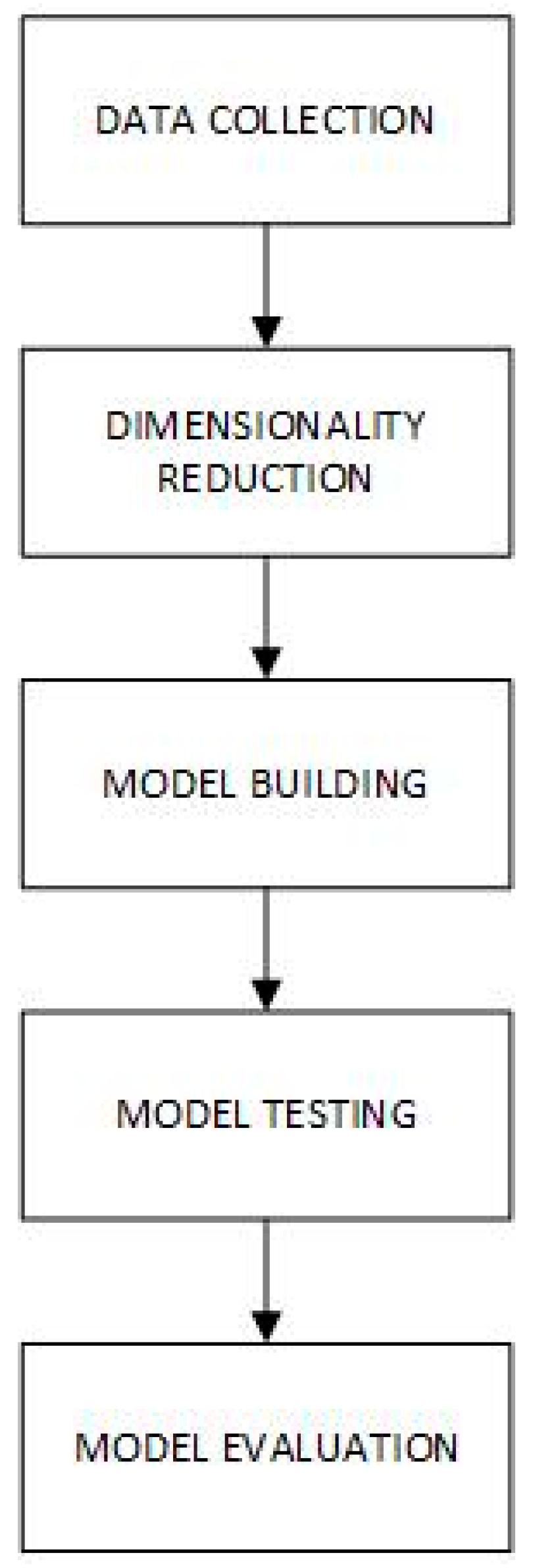
The stages involved in arriving at the final solution comprise of the following: data collection, dimensionality reduction, model building, model testing, and model evaluation. Figure 1 represents the flow of the stages involved in the system methodology, starting with data collection to the model evaluation stage, which is explained in more detail in the following subsections.
3.1. Dataset
The collection of a representative dataset is very important for machine learning to achieve success. This is because a machine learning model has to be trained on a dataset that accurately depicts the conditions for real-world applications of the model. For this model, we used a dataset that contained malicious and benign program data from Windows Portable Executable (PE) files, obtained from Kaggle. The dataset had 19,611 malicious samples obtained from various malware repositories including VirusShare, and benign samples. The dataset originally had 77 features, which included the following:
- NumberOfSections: this refers to the size of the section table, which directly succeeds the headers. This feature is different in both malware and non-malware files.
- MajorLinkerVersion: this is a field in the optional header, and it is the linker major version number.
- AddressOfEntryPoint: this is also a field in the optional header. It is the entry point address. This address is related to the image base obtained as the Portable Executable (PE) file is loaded into memory. It is the starting address for program images, and it is the initialization function address for device drivers. For dynamic-link library (DLL), an entry point is not required. The field is null when there is no entry point.
- ImageBase: this represents the address of the first byte of the image when it loaded into memory. This is usually a multiple of 64K.
- MajorOperatingSystemVersion: a number used to identify the version of the operating system.
- MajorImageVersion: a number used to identify the version of the image. Many benign files have more versions and most malicious files have this feature with a value of zero.
- CheckSum: 90% of the time, when the CheckSum, MajorImageVersion, and DLLCharacteristics of a file are equal to zero, the file is found to be malicious.
- SizeOfImage: this refers to the image size as it is loaded in memory.
The discussed features, along with the class label (0 for benign and 1 for malicious), were used to create the classification model.
3.2. Dimensionality Reduction
Machine learning techniques are applied widely to address a range of prediction and classification problems. Poor performance in machine learning can be caused by overfitting or underfitting the data. Removing the unimportant features ensures the optimum performance of the algorithms and increases the speed. To perform feature dimensionality reduction, principal component analysis (PCA) was applied. Based on previous research, 55 features (representing 95% of variability) were selected to be passed into the machine learning model because the features were proven to be relevant in learning whether a file was malicious or benign.
3.3. Baseline Machine Learning Models
The study employed five machine learning algorithms—namely: random forest, naïve Bayes, AdaBoost, decision tree, and gradient boosting. A brief description of the algorithms is presented below.
A Gaussian naïve Bayes (NB) model [41] is premised on probability and likelihood. The algorithm is stable, fast, and simple. NB is built based on Bayes’ theorem, which is premised on the strong assumption of conditional independence. The assumption is that every feature in a particular class is independent of all other features in that same class. The model is useful when working with very large datasets, and it is easy to build. It can also perform better than other classification algorithms.
The NB algorithm performs well with categorical input variables but performs less well with numerical values and in multi-class classification /prediction. Additionally, the assumption of independence feature upon which the algorithm is based may not always be true.
The decision tree (DT) algorithm [42] performs well for continuous as well as categorical variables. DT classifiers learn to make predictions on the test data by following a tree-like model (created using the training dataset) that resembles a flow chart, based on the features passed into it. Each of the tree’s internal nodes correlates with an attribute, and every leaf node correlates with a class label. In a DT, the best feature of the dataset is positioned at the root of the tree, while the training dataset is divided into subsets. These two steps are then repeated on every subset until there are no further divisions possible. It is a simple algorithm that can work well with large datasets.
Random forest (RF) [43] is a classification algorithm that consists of multiple decision trees that make predictions based on the mean probabilistic prediction of each tree. It is similar to decision trees and it reduces the problem of overfitting, which is a problem associated with the DT algorithm. But it is not easy to interpret, unlike a decision tree. It uses randomness when constructing each DT to create a forest of different trees.
Boosting is a method of making strong learners out of weak learners by combining weak classifiers into one strong classifier. AdaBoost or adaptive boosting [44] is a machine learning classification algorithm that is based on the idea of iteratively making weak learners learn a bigger part of the examples in the training data that are difficult to classify by giving more weight (paying more attention) to examples that are often misclassified. The weak learners consist of DTs with one split, which are called decision stumps.
The gradient boosting (GB) algorithm [45] creates a model as a result of the combination of weaker models. The idea behind gradient boosting is to repeatedly minimize the loss function until the minimum test loss is reached. The steps involved in GB include the following:
- Model the data with simple models and examine the data for errors.
- The errors connote data points that are not easy to fit by a simple model.
- For subsequent models, the focus is placed on improving the accuracy of classification on data that are hard to fit.
- Finally, all the predictors are combined by giving each predictor some weights.
3.4. Deep Learning Models
3.4.1. Multilayer Perceptron
Let the output of a simple multilayer perceptron (MLP) be known as at the input To find model parameters and , , such that the model output would match closely the real value of . The relationship between the input and output of an MLP is established by:
A perceptron with one hidden layer can approximate any continuous function defined on a bounded set as follows:
The training of MLP is performed by applying a gradient descent algorithm (such as error backpropagation).
3.4.2. One-Dimensional (1D) CNN Model
Although the CNN models were primarily designed for image processing, where the model learns an internal representation of a two-dimensional input (2D), the same mechanism can be used for feature learning on 1D data series, such as in the case of malware recognition. The model learns how to derive features from observation sequences and how to map hidden layers to various software types (malicious or benign).
The convolutional layer is the main block of the CNN. The parameters of this layer are a set of trainable filters (scan windows). Each filter works over a small window in size. During forward propagation (from the first layer to the last), the scanning window sequentially traverses the entire image following the tiling principle and calculates dot products of two vectors: the filter values and the outputs of the selected neurons. After passing all the shifts in the width and height of the input volume, a 2D activation map is created, which applies a specific filter in each spatial region. The network uses filters that are activated when on some type of input signal. Each convolutional layer uses a set of filters, and each creates a separate activation map.
Another element of a CNN is the down-sampling or subsampling layer. Usually, it is placed between successive layers of convolution so it can occur periodically. Its function is to gradually decrease the spatial size of the vector in order to decrease the number of computations in the network, as well as to balance overfitting. The convolution layer resizes the feature map, most often using the max pooling operation. The flattening layer is used if the output from the previous layer is to be transmitted to the fully-connected (FC) layer, then it needs to be flattened. The parametric rectified linear unit (PReLU) layer is a neuron activation function that supplements the rectified unit with a slope for negative values.
To regularize the network, the dropout layer is used. It also allows for the network size to be thinner. The neurons that are less likely to boost learning and classification weights are randomly dropped. As there are two classes, this dropout layer is followed by a completely connected (dense) layer that will reduce the output to two classes, and we expect to forecast the actions of the program as either malicious or benevolent. Softmax, which reduces the two outputs to one is the final activation function.
3.5. Ensemble Learning
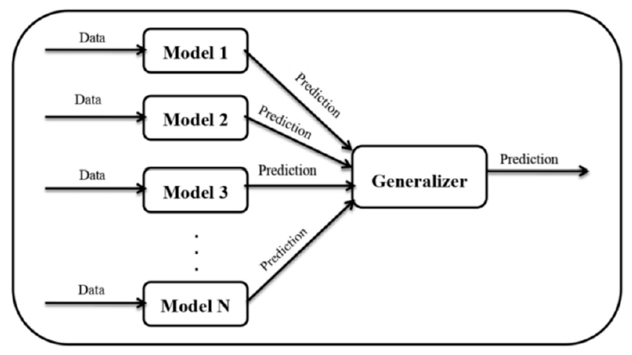
The theory of ensemble methods is that training data are analyzed in multiple ways, and an ensemble of first-stage classifiers is constructed. After that, by integrating the decisions of all those first-stage classifiers, a new ensemble classifier is created using the stacked ensemble approach where a final-stage model learns how to best combine the predictions from multiple first-stage models. We use a stacking approach [46] that has two stages (see Figure 2). First, first-staged on a dataset, multiple models are trained. To create a new dataset, the prediction of each of the first-stage models is then stored. Each instance in the current dataset is connected to the actual value it is expected to estimate. Second, to derive the final prediction, the dataset is used with the meta-learning algorithm.
Base models (also referred to as first-stage models) and a meta-learner (or, final-stage classifier) that incorporates base model predictions make up a stacking model. Different first-stage models are trained on the training data. Next, the final-stage model is trained on the training dataset and the outputs of the first-stage models to combine the base model predictions using previously unused data.
The ensemble learner algorithm consists of three phases:
- Create the ensemble
- Select different base classifiers.
- Select a final-stage classifier.
- Train the ensemble
- Train each of the first-stage classifiers on the training dataset.
- Perform k-fold cross-validation on each of the first-stage classifiers and record their decisions.
- Combine the decisions from the first-stage classifiers to form a feature matrix:
- Train the final-stage classifier on the new (features x predictions) data. Then the ensemble model combines the first-stage learning models and the final-stage model, to get more accurate predictions on unknown data.
- Test on new data.
- Store output predictions from the first-stage classifiers.
- Input first-stage classifier decisions into a final-stage classifier to make a final ensemble prediction.
The algorithm of ensemble learning is summarized as an algorithm in Algorithm 1. Stacking improves over any single best learner on the training dataset. When first-stage classifiers used for stacking have variable and uncorrelated outputs, the largest gains in performance are typically made.
| Algorithm 1. Pseudocode of the ensemble learning algorithm. |
 |
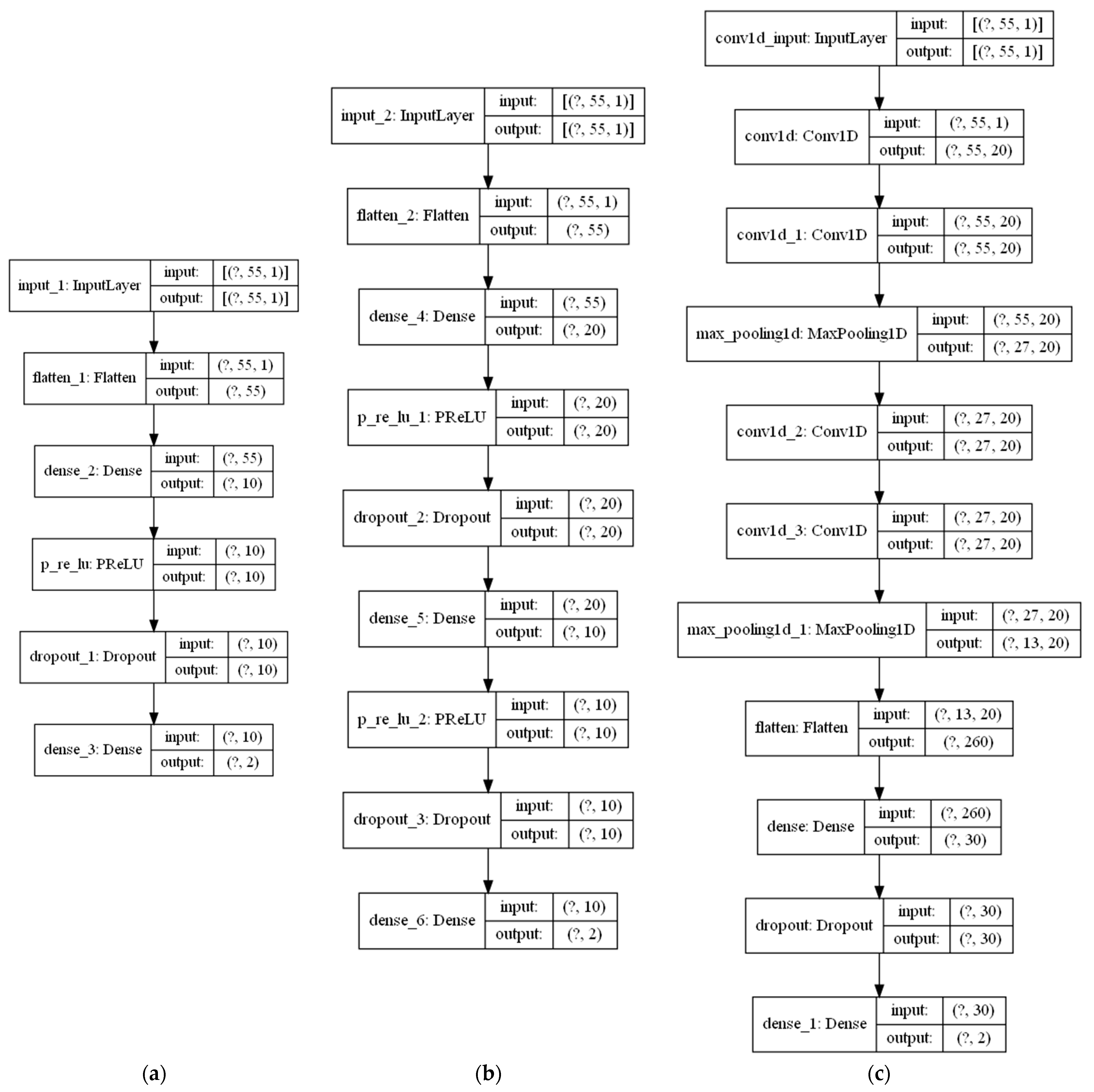
As first-stage classifiers, we used fully connected one hidden layer MLPs (Dense-1), fully connected two hidden layer MLPs (Dense-2), and one-dimensional CNNs (1D-CNN). The configurations of neural networks are given in Table 1. The instances of ANN model architectures are shown in Figure 3a–c.
As final-stage classifiers, we analyzed decision tree (DT), support vector machine (SVM) with linear and radial basis function (RBF) kernels, random forest (RF), k-nearest neighbors (KNN), multilayer perceptron (MLP), AdaBoost classifier, ExtraTrees (ET) classifier, isolation forest (IF), Gaussian naïve Bayes (NB), linear discriminant analysis (LDA), quadratic discriminant analysis (QDA), logistic regression (LR), passive-aggressive classifier (PAC), ridge classifier (RC), and stochastic gradient descent (SGD) classifiers.
K-nearest neighbors (KNN) classifies unseen input data based on the known input data that are most similar (close) to it. Support vector machine (SVM) is a supervised learning technique that creates a hyperplane in a higher dimension to separate input data belonging to different classes while maximizing the distance of input data to the hyperplane. The ExtraTrees classifier (ET) [47] constructs a meta estimator that fits several decision trees on sub-samples of the training dataset and employs averaging to increase accuracy and manage over-fitting. Linear discriminant analysis (LDA) aims to find a linear combination of input features that separates two or more classes of input data. Quadratic discriminant analysis (QDA) uses a quadratic decision surface to separate two or more classes of input data. Logistic regression (LR) is a statistical method similar to linear regression that predicts an outcome for a binary output variable from input variables. Passive-aggressive classifier (PAC) [48] is one of the incremental learning algorithms that adjusts its weight vector for each misclassified training sample it receives, trying to get it correct. Ridge classifier (RC) converts the label data into [−1, 1] and solves the problem with the regression method. The highest value in prediction is accepted as a target class. Stochastic gradient descent (SGD) classifier is a SGD learning algorithm that finds the decision boundary with hinge loss similar to a linear SVM.
3.6. Evaluation
The performance of the proposed model was evaluated using leave-one-out cross-validation (LOOCV) with 10-fold cross-validation. The true labels were matched against the predicted labels and recall, precision, accuracy, error rate, F-score, and Matthews correlation coefficient (MCC) values were calculated as given in Table 2 (we assumed a binary classification problem):
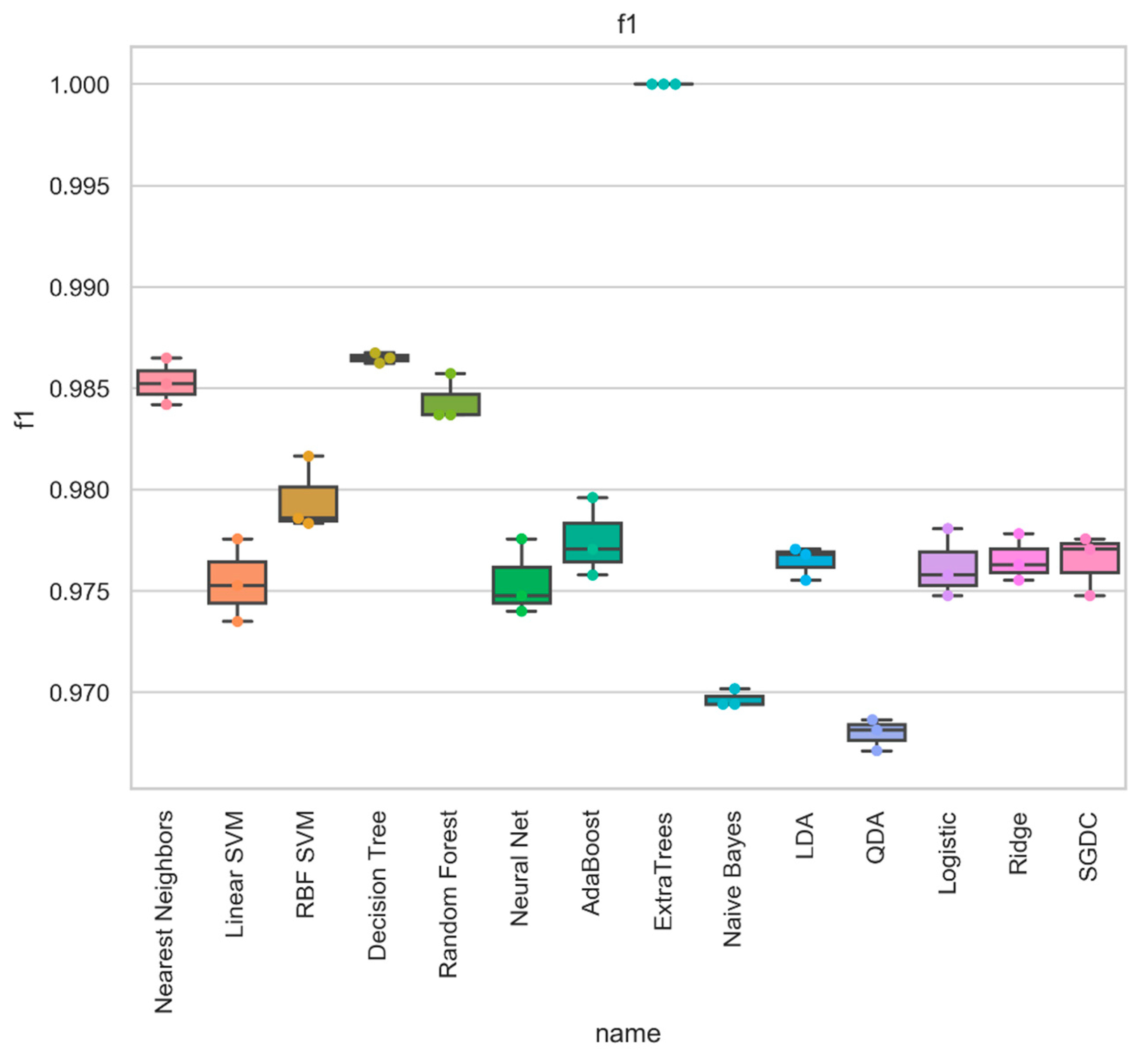
According to the F1-score, we chose the best model instead of testing the model with accuracy alone. This was since, in datasets where a significant class imbalance occurs, accuracy can be a misleading metric. For example, for all predictions, a model will correctly predict the value of the majority class and achieve a high classification performance while making errors in the minority and main classes. This form of conduct is penalized by the F1-score by measuring the metrics for each label and finding its unweighted average.
We also considered Area Under Curve (AUC) as a measure of the quality of binary classification that is considered as a balanced metric that can be used for highly imbalanced datasets.
The Cohen’s kappa is calculated by:
where is the ratio of correct agreement, and is the ratio of agreement that is predicted by random choice.
Apart from this, the performance of the proposed model on a binary dataset is represented using the confusion matrix as follows:
Here, represents the number of elements belonging to the i-th class () but that are classified as members of the j-th class ().
The random guess classifier and the zero rule classifier were adopted as baseline classifiers. In the dataset, the zero rule classifier returned the majority class only. The accuracy of a random guess classifier is calculated as follows:
where is the probability of the i-th class, and is the number of samples of class .
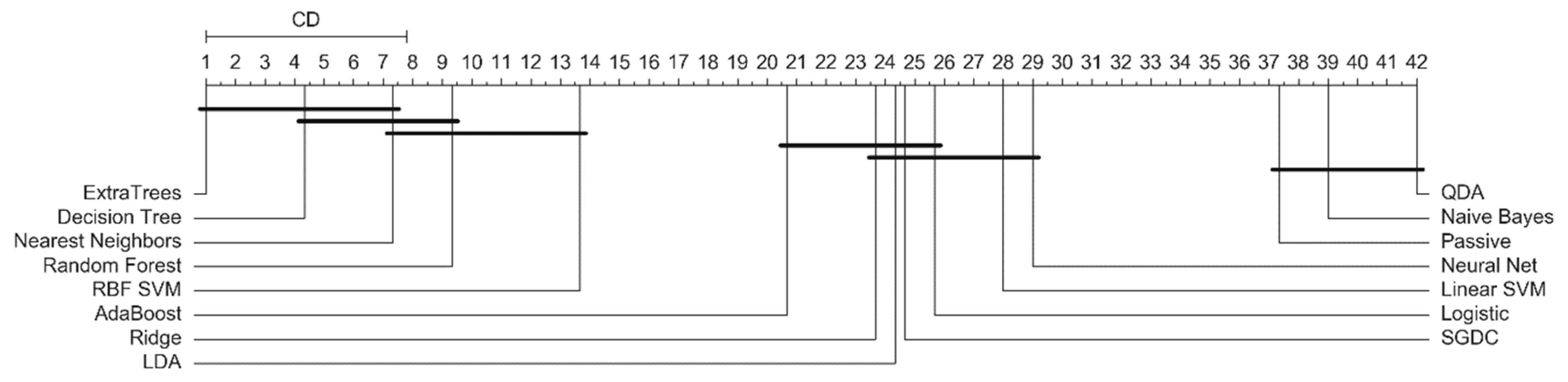
For statistical analysis, we used the performance results obtained from each fold of the 10-fold cross-validation. To compare the results and evaluate their statistical significance, we used the Friedman test and post hoc Nemenyi test. First, all methods were ranked based on some selected performance measures (we used accuracy, AUC, and F1-score). Then, the mean ranks of each method were calculated. The difference between method performance was considered as not significant if the difference between mean ranks of the methods was smaller than the critical difference derived from the Nemenyi test.
4. Results
4.1. Ssettings of Experiments
The classifiers were trained using the features extracted from the dataset using Python’s Scikit-learn. All experiments were executed on a laptop computer with 64-bit Windows 10 OS with Intel Core i5-8265U CPU 1.80 GHz with 8GB RAM.
4.2. Results of Machine Learning Methods
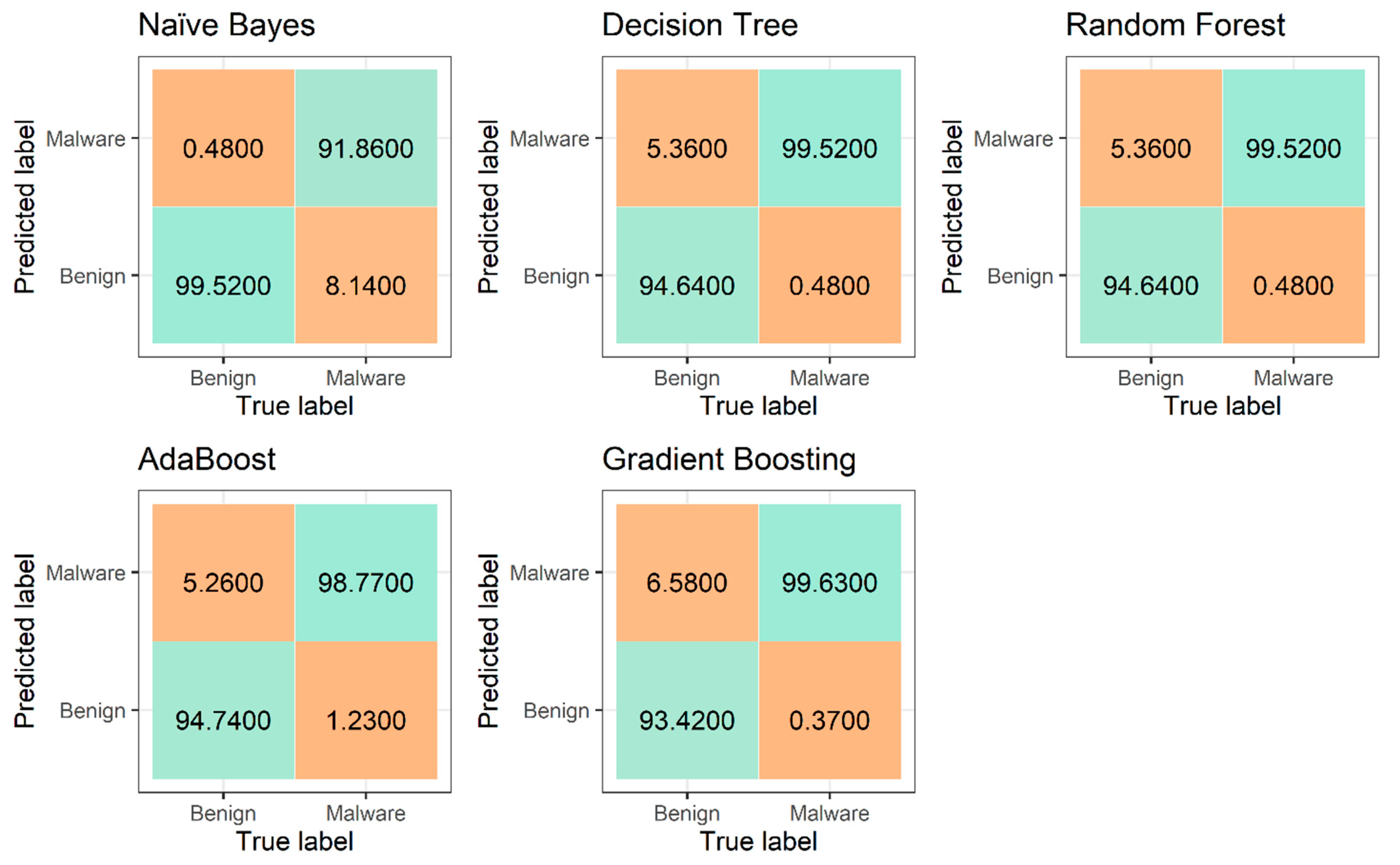
The results achieved from using baseline machine learning methods are presented in Table 3, while their confusion matrices are given in Figure 4. The best results were the false positive and false negative rates of 2.13% and 0.31%, respectively, obtained by the RF model. The accuracy of 99.24% and F1 score of 0.98 indicate that RF classified instances of each of the two classes quite well. For comparison, the accuracy of the random guess classifier on this dataset was 61.9%, whereas the accuracy of the zero rule classifier was 74.4%.
4.3. Results of Neural Network Models
To select the first-stage classifiers, first, we performed an ablation study to find the best Dense-1, Dense-2, and 1D-CNN models considering their performance for different settings of their hyperparameters. Note that in all experiments we used sparse categorical cross-entropy loss and Adam optimizer. Eighty percent of the data was used for training and 20% for testing. The results are shown in Table 4, Table 5 and Table 6. We trained Dense-1 and Dense-2 models for 200 epochs, while the 1D-CNN models were trained for 50 epochs.
4.4. Results of Ensemble Classification
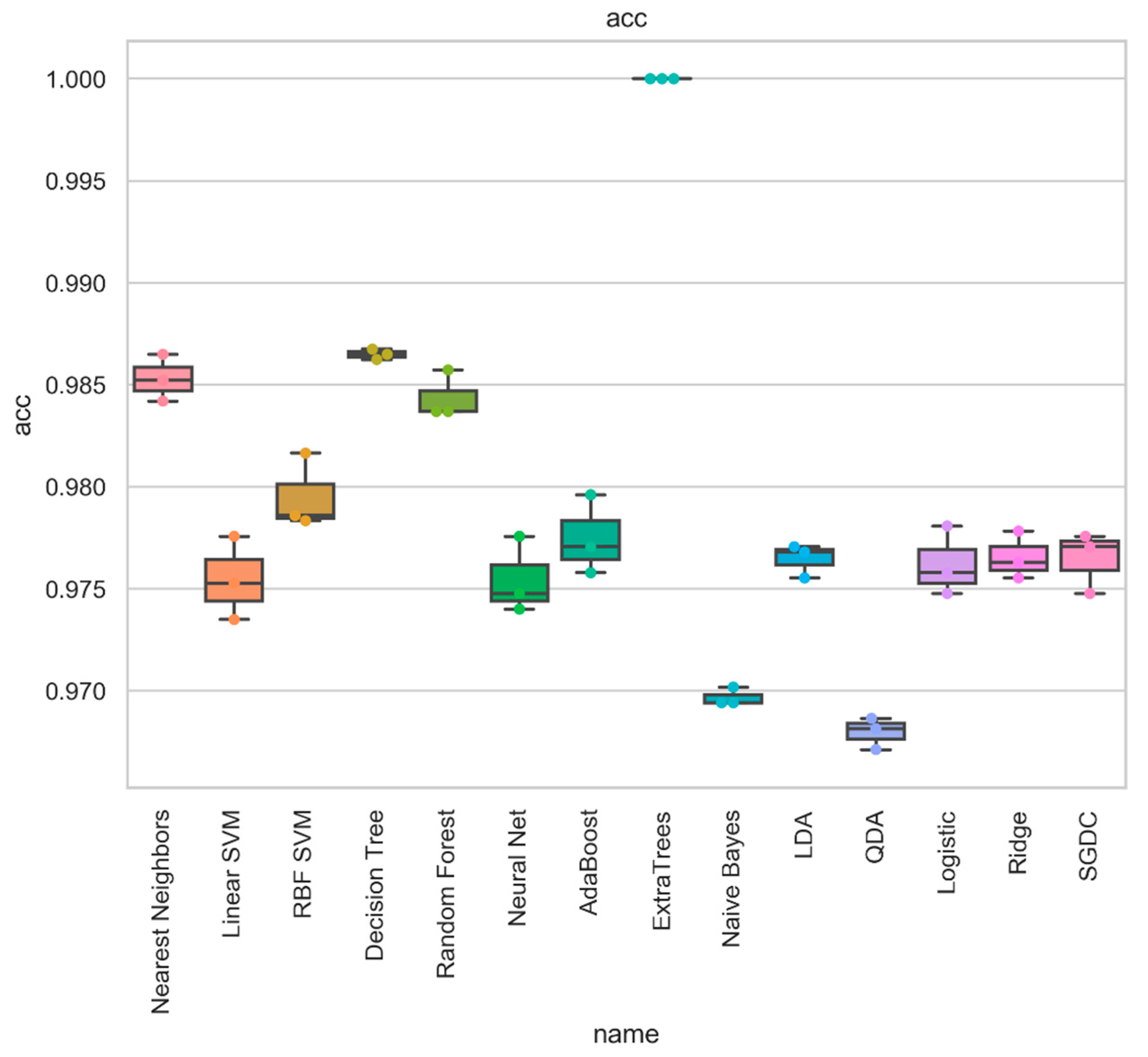
Based on the presented ablation study, we selected two Dense-1 (with 35 and 50 neurons) models, two Dense-2 (with (40;40) and (40;50) neurons) models, and 3 1D-CNN ((20;60), (60;40), (60;60)) models as first-stage classifiers based on their higher performance results. We performed classification with several last-stage classifiers. For KNN, the number of nearest neighbors was set to 3. For linear SVM, C was set to 0.025. For RBF SVM, the C parameter was set to 1, and gamma was set to 2. For DT and RF, the max depth was set to 5. The results are given in Table 7. In all experiments, 10-fold cross-validation was used, where the training fold was constructed by selecting 80% of samples, while 20% were used for the testing fold.
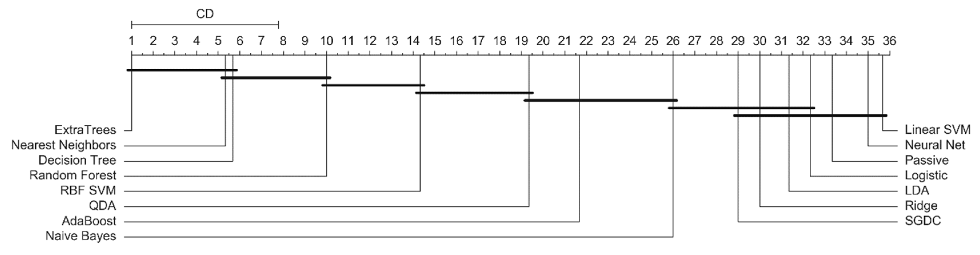
4.5. Statistical Analysis
To analyze the results statistically, we adopted the nonparametric Friedman test and post hoc Nemenyi test. The testing results are the critical difference (CD) diagrams presented in Figure 8, Figure 9 and Figure 10. If the difference between the mean ranks of the final-stage classifiers was smaller than the CD, then it was not statistically significant. The results of the Nemenyi test again show that the ExtraTrees final-stage classifier allowed achieving the best performance; however, DT and KNN classifiers presented statistically similar performance.
4.6. Comparison with Previous Work
We compare the results of our experiments with some of the previous work on classifying benign and malware files in Table 8. Note that the methods applied on different malware datasets are compared. In the same dataset, the previous best result was achieved in [49] using XGBoost with an accuracy of 98.62%.
5. Conclusions
There is a rise in demand for intelligent methods that recognize new malware cases because the current methods are tedious and error-prone. This study explored various machine learning classifiers and neural network models, which are artificial intelligence methods that can be used for detecting malware. We proposed an ensemble learning-based framework with neural networks used as first-stage classifiers and explored 15 machine learning models as final-stage classifiers. Five different machine learning algorithms were used for comparison as baseline models. We performed our experiments on a dataset containing Windows Portable Executable (PE) malware and benign files. The results obtained indicate that the ensemble of fully connected dense ANN and 1-D CNN models with ExtraTrees as a final-stage classifier achieved the best accuracy value for the classification process, outperforming other methods.
Most of the known malware recognition methods concentrate on featuring engineering techniques to improve detection accuracy; the advantage of our deep learning-based approach is the end-to-end learning process without the need for manual feature engineering to achieve high malware recognition performance. Thus, ensemble learning techniques can be adopted as intelligent techniques for malware detection and classification. However, the proposed framework is limited to supervised learning, which required both benign and malicious malware to be identified and labeled by experts. In the real-world setting, some malicious code may not be identified and thus the neural network cannot be trained on recognizing it. This raises the need for developing unsupervised ensemble learning frameworks for malware recognition.
Future work will perform the study of explainable artificial intelligence (XAI) techniques to interpret the results of deep learning models for malware recognition to provide valuable insights for researchers in malware analysis. We also plan to conduct additional experiments with larger datasets to validate the proposed framework.
Author Contributions
Conceptualization, N.A.A., S.M., and R.D.; methodology, S.M. and R.D.; software, N.A.A., O.E.O., J.O., and R.D.; validation, N.A.A., S.M., and R.D.; formal analysis, N.A.A. and R.D.; investigation, N.A.A., O.E.O., S.M., J.O., and R.D.; resources, N.A.A. and S.M.; writing—original draft preparation, N.A.A., O.E.O., and J.O.; writing—review and editing, S.M. and R.D.; visualization, N.A.A. and R.D.; supervision, S.M. All authors have read and agreed to the published version of the manuscript.
Funding
This research received no external funding.
Institutional Review Board Statement
Not applicable.
Informed Consent Statement
Not applicable.
Data Availability Statement
The dataset is available from https://www.kaggle.com/amauricio/pe-files-malwares (accessed on 10 February 2021).
Conflicts of Interest
The authors declare no conflict of interest.
References
- International Telecommunication Union. Statistics. Available online: https://www.itu.int/en/ITU-D/Statistics/Pages/publications/yb2018.aspx (accessed on 20 November 2019).
- Namanya, A.P.; Cullen, A.; Awan, I.U.; Disso, J.P. The World of Malware: An Overview. In Proceedings of the IEEE 6th International Conference on Future Internet of Things and Cloud (FiCloud 2018), Barcelona, Spain, 6–8 August 2018; pp. 420–427. [Google Scholar] [CrossRef]
- Gilbert, D.; Mateu, C.; Planes, J. The rise of machine learning for detection and classification of malware: Research developments, trends and challenges. J. Netw. Comput. Appl. 2020, 153, 102526. [Google Scholar] [CrossRef]
- Subairu, S.O.; Alhassan, J.; Misra, S.; Abayomi-Alli, O.; Ahuja, R.; Damasevicius, R.; Maskeliunas, R. An experimental approach to unravel effects of malware on system network interface. In Advances in Data Sciences, Security and Applications; Lecture Notes in Electrical Engineering; Springer: Singapore, 2020; Volume 612, pp. 225–235. [Google Scholar] [CrossRef]
- Azeez, N.A.; Salaudeen, B.B.; Misra, S.; Damasevicius, R.; Maskeliunas, R. Identifying phishing attacks in communication networks using URL consistency features. Int. J. Electron. Secur. Digit. Forensics 2020, 12, 200–213. [Google Scholar] [CrossRef]
- Yong, B.; Wei, W.; Li, K.; Shen, J.; Zhou, Q.; Wozniak, M.; Damaševičius, R. Ensemble machine learning approaches for webshell detection in internet of things environments. Trans. Emerg. Telecommun. Technol. 2020. [Google Scholar] [CrossRef]
- Wei, W.; Woźniak, M.; Damaševičius, R.; Fan, X.; Li, Y. Algorithm research of known-plaintext attack on double random phase mask based on WSNs. J. Internet Technol. 2019, 20, 39–48. [Google Scholar] [CrossRef]
- Boukhtouta, A.; Mokhov, S.A.; Lakhdari, N.-E.; Debbabi, M.; Paquet, J. Network malware classification comparison using dpi and flow packet headers. J. Comput. Virol. Hacking Tech. 2016, 12, 69–100. [Google Scholar] [CrossRef]
- Zatloukal, J.Z. Malware Detection Based on Multiple PE Headers Identification and Optimization for Specific Types of Files. J. Adv. Eng. Comput. 2017, 1, 153–161. [Google Scholar] [CrossRef] [Green Version]
- Odusami, M.; Abayomi-Alli, O.; Misra, S.; Shobayo, O.; Damasevicius, R.; Maskeliunas, R. Android malware detection: A survey. In Applied Informatics. ICAI 2018; Springer: Cham, Switzerland, 2018; Volume 942, pp. 255–266. [Google Scholar] [CrossRef]
- Gardiner, J.; Nagaraja, S. On the security of machine learning in malware detection: A survey. ACM Comput. Surv. 2016, 49, 1–39. [Google Scholar] [CrossRef] [Green Version]
- Ye, Y.; Li, T.; Adjeroh, D.; Iyengar, S.S. A survey on malware detection using data mining techniques. ACM Comput. Surv. 2017, 50, 1–40. [Google Scholar] [CrossRef]
- Souri, A.; Hosseini, R. A state-of-the-art survey of malware detection approaches using data mining techniques. Hum. Centric Comput. Inf. Sci. 2018, 8, 3. [Google Scholar] [CrossRef]
- Ucci, D.; Aniello, L.; Baldoni, R. Survey of machine learning techniques for malware analysis. Comput. Secur. 2019, 81, 123–147. [Google Scholar] [CrossRef] [Green Version]
- Sathyanarayan, V.S.; Kohli, P.; Bruhadeshwar, B. Signature Generation and Detection of Malware Families. In Information Security and Privacy, Proceedings of the Australasian Conference on Information Security and Privacy, ACISP 2008, Wollongong, Australia, 7–9 July 2008; Mu, Y., Susilo, W., Seberry, J., Eds.; Lecture Notes in Computer, Science; Springer: Berlin/Heidelberg, Germany, 2008; Volume 5107, pp. 336–349. [Google Scholar]
- Zhong, W.; Gu, F. A multi-level deep learning system for malware detection. Expert Syst. Appl. 2019, 133, 151–162. [Google Scholar] [CrossRef]
- Vinayakumar, R.; Alazab, M.; Soman, K.P.; Poornachandran, P.; Venkatraman, S. Robust intelligent malware detection using deep learning. IEEE Access 2019, 7, 46717–46738. [Google Scholar] [CrossRef]
- Venkatraman, S.; Alazab, M.; Vinayakumar, R. A hybrid deep learning image-based analysis for effective malware detection. J. Inf. Secur. Appl. 2019, 47, 377–389. [Google Scholar] [CrossRef]
- Lu, T.; Du, Y.; Ouyang, L.; Chen, Q.; Wang, X. Android malware detection based on a hybrid deep learning model. Secur. Commun. Netw. 2020. [Google Scholar] [CrossRef]
- Yoo, S.; Kim, S.; Kim, S.; Kang, B.B. AI-HydRa: Advanced hybrid approach using random forest and deep learning for malware classification. Inf. Sci. 2021, 546, 420–435. [Google Scholar] [CrossRef]
- Nisa, M.; Shah, J.H.; Kanwal, S.; Raza, M.; Khan, M.A.; Damaševičius, R.; Blažauskas, T. Hybrid malware classification method using segmentation-based fractal texture analysis and deep convolution neural network features. Appl. Sci. 2020, 10, 4966. [Google Scholar] [CrossRef]
- Bazrafshan, Z.; Hashemi, H.; Fard, S.M.H.; Hamzeh, A. A survey on heuristic malware detection techniques. In Proceedings of the 5th Conference on Information and Knowledge Technology (IKT), Shiraz, Iran, 28–30 May 2013; pp. 113–120. [Google Scholar]
- Rathore, H.; Agarwal, S.; Sahay, S.; Sewak, M. Malware Detection using Machine Learning and Deep Learning. In Proceedings of the International Conference of Big Data Analytics, Goa, India, 17–20 December 2019; Springer: Cham, Switzerland, 2019; pp. 402–411. [Google Scholar]
- Lee, Y.-S.; Lee, J.-U.; Soh, W.-Y. Trend of Malware Detection Using Deep Learning. In Proceedings of the 2nd International Conference on Education and Multimedia Technology, Okinawa, Japan, 2–4 July 2018; pp. 102–106. [Google Scholar]
- Pluskal, O. Behavioural malware detection using efficient SVM implementation. In Proceedings of the Conference on Research in Adaptive and Convergent Systems—RACS, Prague, Czech Republic, 9–12 October 2015; pp. 296–301. [Google Scholar] [CrossRef]
- Cakir, B.; Dogdu, E. Malware classification using deep learning methods. In Proceedings of the ACMSE 2018 Conference on—ACMSE ’18, Richmond, KY, USA, 29–31 March 2018. [Google Scholar] [CrossRef]
- Ren, Z.; Wu, H.; Ning, Q.; Hussain, I.; Chen, B. End-to-end malware detection for android IoT devices using deep learning. Ad Hoc Netw. 2020, 101, 102098. [Google Scholar] [CrossRef]
- Yuxin, D.; Siyi, Z. Malware detection based on deep learning algorithm. Neural Comput. Appl. 2019, 31, 461–472. [Google Scholar] [CrossRef]
- Pei, X.; Yu, L.; Tian, S. AMalNet: A deep learning framework based on graph convolutional networks for malware detection. Comput. Secur. 2020, 93, 101792. [Google Scholar] [CrossRef]
- Čeponis, D.; Goranin, N. Investigation of dual-flow deep learning models LSTM-FCN and GRU-FCN efficiency against single-flow CNN models for the host-based intrusion and malware detection task on univariate times series data. Appl. Sci. 2020, 10, 2373. [Google Scholar] [CrossRef] [Green Version]
- Huang, X.; Ma, L.; Yang, W.; Zhong, Y. A method for windows malware detection based on deep learning. J. Signal Process. Syst. 2021, 93, 265–273. [Google Scholar] [CrossRef]
- Abiodun, O.I.; Kiru, M.U.; Jantan, A.; Omolara, A.E.; Dada, K.V.; Umar, A.M.; Linus, O.U.; Arshad, H.; Kazaure, A.A.; Gana, U. Comprehensive Review of Artificial Neural Network Applications to Pattern Recognition. IEEE Access 2019, 7, 158820–158846. [Google Scholar] [CrossRef]
- Dai, Y.; Li, H.; Qian, Y.; Yang, R.; Zheng, M. SMASH: A malware detection method based on multi-feature ensemble learning. IEEE Access 2019, 7, 112588–112597. [Google Scholar] [CrossRef]
- Khasawneh, K.N.; Ozsoy, M.; Donovick, C.; Abu-Ghazaleh, N.; Ponomarev, D. EnsembleHMD: Accurate hardware malware detectors with specialized ensemble classifiers. IEEE Trans. Dependable Secur. Comput. 2018, 17, 620–633. [Google Scholar] [CrossRef] [Green Version]
- Li, D.; Li, Q. Adversarial deep ensemble: Evasion attacks and defenses for malware detection. IEEE Trans. Inf. Forensics Secur. 2020, 15, 3886–3900. [Google Scholar] [CrossRef]
- Xue, D.; Li, J.; Wu, W.; Tian, Q.; Wang, J. Homology analysis of malware based on ensemble learning and multifeatures. PLoS ONE 2019, 14, e0211373. [Google Scholar] [CrossRef] [PubMed]
- Zhang, J.; Gao, C.; Gong, L.; Gu, Z.; Man, D.; Yang, W.; Li, W. Malware detection based on multi-level and dynamic multi-feature using ensemble learning at hypervisor. Mobile Netw. Appl. 2020. [Google Scholar] [CrossRef]
- Galar, M.; Fernandez, A.; Barrenechea, E.; Bustince, H.; Herrera, F. A review on ensembles for the class imbalance problem: Bagging-, boosting-, and hybrid-based approaches. IEEE Trans. Syst. Man Cybern. Part C Appl. Rev. 2012, 42, 463–484. [Google Scholar] [CrossRef]
- Sagi, O.; Rokach, L. Ensemble learning: A survey. Wiley Interdiscip. Rev. Data Min. Knowl. Discov. 2018, 8. [Google Scholar] [CrossRef]
- Basu, I. Malware detection based on source data using data mining: A survey. Am. J. Adv. Comput. 2016, 3, 18–37. [Google Scholar]
- Zhang, H. The optimality of naive bayes. In Proceedings of the Seventeenth International Florida Artificial Intelligence Research Society Conference, FLAIRS 2004, Miami Beach, FL, USA, 12–14 May 2004; AAAI Press: Menlo Park, CA, USA, 2004; Volume 2, pp. 562–567. [Google Scholar]
- Quinlan, J.R. Induction of decision trees. Mach. Learn. 1986, 1, 81–106. [Google Scholar] [CrossRef] [Green Version]
- Breiman, L. Random forests. Mach. Learn. 2001, 45, 5–32. [Google Scholar] [CrossRef] [Green Version]
- Rätsch, G.; Onoda, T.; Müller, K.R. Regularizing AdaBoost. In Advances in Neural Information Processing Systems; MIT Press: Cambrigde, MA, USA, 1999; pp. 564–570. [Google Scholar]
- Friedman, J.H. Greedy function approximation: A gradient boosting machine. Ann. Stat. 2001, 29, 1189–1232. [Google Scholar] [CrossRef]
- Van der Laan, M.J.; Polley, E.C.; Hubbard, A.E. Super Learner. Stat. Appl. Genet. Mol. Biol. 2007, 6. [Google Scholar] [CrossRef] [PubMed]
- Geurts, P.; Ernst, D.; Wehenkel, L. Extremely Randomized Trees. Mach. Learn. 2006, 63, 3–42. [Google Scholar] [CrossRef] [Green Version]
- Crammer, K.; Dekel, O.; Keshet, J.; Shalev-Shwartz, S.; Singer, Y. Online Passive-Aggressive Algorithms. J. Mach. Learn. Res. 2006, 7, 551–585. [Google Scholar]
- Azmee, A.B.M.; Protim, P.; Aosaful, M.; Dutta, O.; Iqbal, M. Performance Analysis of Machine Learning Classifiers for Detecting PE Malware. Int. J. Adv. Comput. Sci. Appl. 2020, 11. [Google Scholar] [CrossRef] [Green Version]
- Yuan, Z.; Lu, Y.; Xue, Y. Droiddetector: Android malware characterization and detection using deep learning. Tsinghua Sci. Technol. 2016, 21, 114–123. [Google Scholar] [CrossRef]
- McLaughlin, N.; Martinez del Rincon, J.; Kang, B.; Yerima, S.; Miller, P.; Sezer, S.; Safaei, Y.; Trickel, E.; Zhao, Z.; Doupe, A.; et al. Deep android malware detection. In Proceedings of the Seventh ACM Conference on Data and Application Security and Privacy, CODASPY 2017, Scottsdale, AZ, USA, 22–24 March 2017; pp. 301–308. [Google Scholar]
- Karbab, E.B.; Debbabi, M.; Derhab, A.; Mouheb, D. Android malware detection using deep learning on api method sequences. arXiv 2017, arXiv:1712.08996. [Google Scholar]
- Hou, S.; Saas, A.; Ye, Y.; Chen, L. DroidDelver: An Android Malware Detection System Using Deep Belief Network Based on API Call Blocks. In Web-Age Information Management; Song, S., Tong, Y., Eds.; Lecture Notes in Computer Science; Springer: Cham, Switzerland, 2016; Volume 9998. [Google Scholar] [CrossRef]
- Hou, S.; Saas, A.; Chen, L.; Ye, Y.; Bourlai, T. Deep neural networks for automatic android malware detection. In Proceedings of the 2017 IEEE/ACM International Conference on Advances in Social Networks Analysis and Mining, Sydney, Australia, 13 July–3 August 2017; pp. 803–810. [Google Scholar]
- Raff, E.; Barker, J.; Sylvester, J.; Brandon, R.; Catanzaro, B.; Nicholas, C.K. Malware detection by eating a whole EXE. In Proceedings of the Workshops of the Thirty-Second AAAI Conference on Artificial Intelligence, New Orleans, LA, USA, 2–7 February 2018; pp. 268–276. [Google Scholar]
- Krčál, M.; Švec, O.; Bálek, M.; Jašek, O. Deep convolutional malware classifiers can learn from raw executables and labels only. In Proceedings of the 6th International Conference on Learning Representations, ICLR 2018, Vancouver, BC, Canada, 30 April–3 May 2018. [Google Scholar]
Figure 1.
Overview of the proposed malware recognition framework.

Figure 2.
Scheme of ensemble classification.

Figure 3.
Architectures of first-stage classifiers: (a) Dense-1 network architecture with 10 neurons in a single hidden layer, (b) Dense-2 network architecture with 20 neurons in a first hidden layer and 10 neurons in a second hidden layer, (c) 1D-CNN network architecture with 20 filters in the convolutional layers, and 30 neurons in the final fully connected layer.

Figure 4.
Confusion matrices of baseline machine learning methods.

Figure 5.
Comparison of performance of ensemble model by final-stage classifier: accuracy.

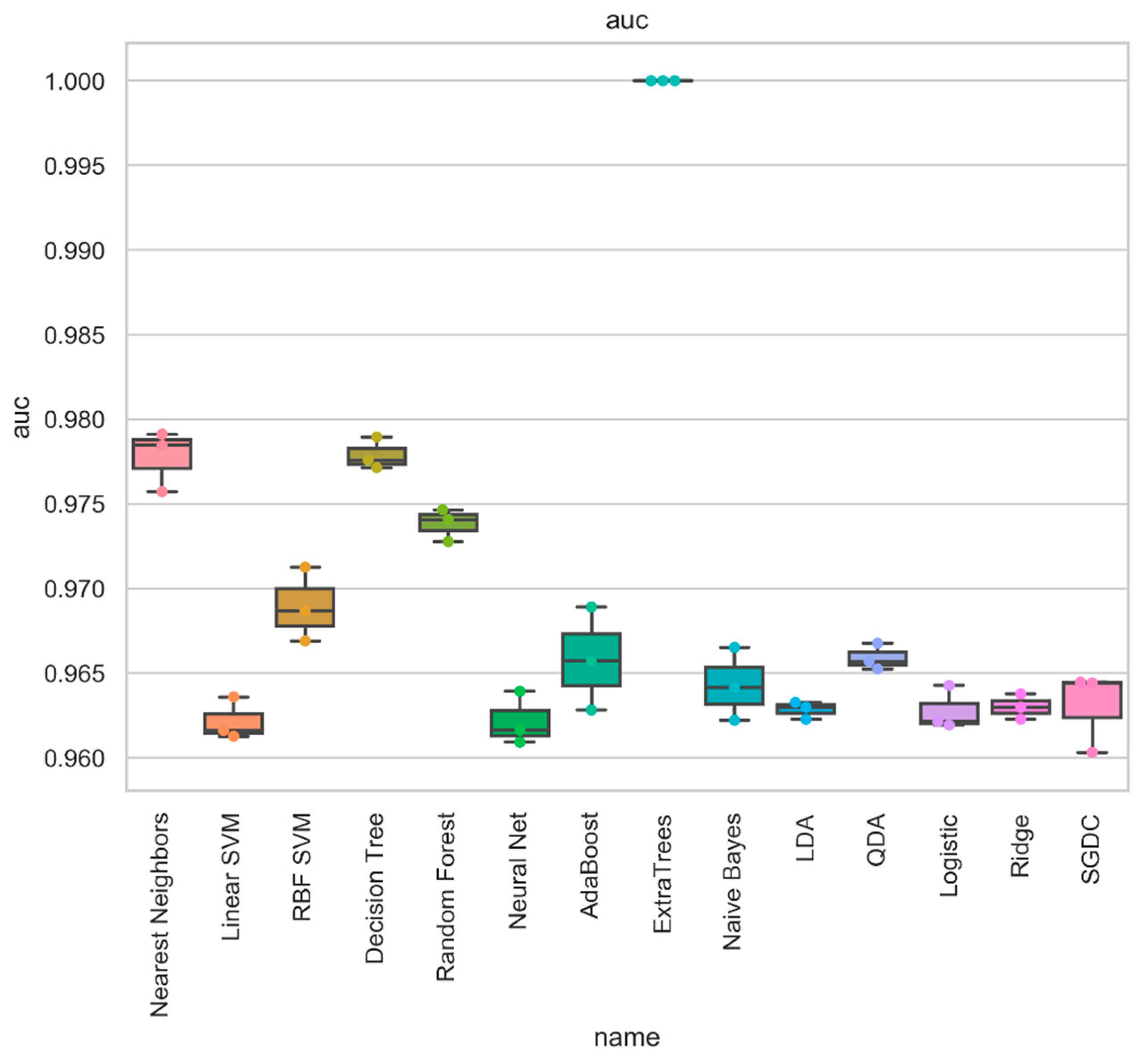
Figure 6.
Comparison of performance of ensemble model by final-stage classifier: Area under Curve.

Figure 7.
Comparison of performance of ensemble model by final-stage classifier: F1-score.

Figure 8.
Comparison of mean ranks of final-stage classifiers based on their accuracy performance.

Figure 9.
Comparison of mean ranks of final-stage classifiers based on their AUC performance.

Figure 10.
Comparison of mean ranks of final-stage classifiers based on their F1-score performance.


Table 1.
Model configuration of neural network with their parameters.
| Dense-1 | Dense-2 | 1D-CNN 1 |
|---|---|---|
| A—number of neurons in 1st hidden layer | A—number of neurons in 1st hidden layer B—number of neurons in 2nd hidden layer | F—number of filters in convolutional layers N—number of neurons in the dense layer |
| Input layer of 55 × 1 features | ||
| 1 FC layer (A neurons) | 1 FC layer (A neurons) | 2 Conv1D layers (F 2 × 2 filters) |
| PReLU 2 | PReLU | Max-pooling layer |
| Dropout layer (p = 0.3) | Dropout layer (p = 0.3) | 2 Conv1D layers (F 2 × 2 filters) |
| 1 FC layer (N neurons) | 1 FC layer (A neurons) | Max-pooling layer |
| Softmax output layer | PReLU | 1 FC layer (N neurons) |
| Dropout layer (p = 0.3) | Dropout layer (p = 0.5) | |
| 1 FC layer (B neurons) | 1 FC layer (2 neurons) | |
| Softmax output layer | Softmax output layer | |
1 1D-CNN—one-dimensional convolutional neural network. 2 PReLU—parametric rectified linear unit.
Table 2.
Summary of performance measures calculated using true positive (TP), false positive (FP), true negative (TN), and false-negative (FN) values.
Table 2.
Summary of performance measures calculated using true positive (TP), false positive (FP), true negative (TN), and false-negative (FN) values.
| Performance Measure | Calculation |
|---|---|
| False Positive Rate (FPR) (also specificity) | |
| True Positive Rate (TPR) (also sensitivity and recall) | |
| False Negative Rate (FNR) | |
| True Negative Rate (TNR) | |
| Precision | |
| F-score | |
| Accuracy | |
| Matthews Correlation Coefficient (MCC) |
Here, is the sum of correctly classified data samples, is the total number of data samples, is classifier with inputs , and are the outputs.
Table 3.
Summary of results of machine learning models.
| Performance Measure | Naïve Bayes | Decision Trees | Random Forest | AdaBoost | Gradient Boosting |
|---|---|---|---|---|---|
| Accuracy | 32.53% | 98.29% | 99.24% | 98.06% | 98.06% |
| Error | 67.47% | 1.71% | 0.76% | 1.94% | 1.94% |
| FPR | 99.52 | 5.36% | 2.13% | 5.26% | 6.58% |
| TPR | 8.14% | 99.52% | 99.69% | 98.77% | 99.63% |
| FNR | 91.86% | 0.48% | 0.31% | 1.23% | 0.37% |
| TNR | 0.48% | 94.64% | 97.87% | 94.74% | 93.42% |
| Precision | 0.28 | 0.99 | 0.99 | 0.96 | 0.99 |
| Recall | 0.99 | 0.95 | 0.98 | 0.95 | 0.93 |
| F-measure | 0.44 | 0.97 | 0.98 | 0.96 | 0.96 |
Table 4.
Deep learning results with a different number of neurons in the hidden layer of the Dense-1 model. Best results are given in bold.
Table 4.
Deep learning results with a different number of neurons in the hidden layer of the Dense-1 model. Best results are given in bold.
| No. of Neurons in 1st Layer | Acc | Prec | Rec | Spec | FPR | FNR | F1 | AUC | MCC | Kappa |
|---|---|---|---|---|---|---|---|---|---|---|
| 5 | 0.968 | 0.968 | 0.968 | 0.968 | 0.068 | 0.02 | 0.968 | 0.956 | 0.915 | 0.915 |
| 10 | 0.97 | 0.97 | 0.97 | 0.97 | 0.065 | 0.018 | 0.97 | 0.959 | 0.921 | 0.921 |
| 15 | 0.978 | 0.978 | 0.978 | 0.978 | 0.054 | 0.011 | 0.978 | 0.967 | 0.942 | 0.942 |
| 20 | 0.98 | 0.98 | 0.98 | 0.98 | 0.054 | 0.009 | 0.98 | 0.968 | 0.945 | 0.945 |
| 25 | 0.978 | 0.978 | 0.978 | 0.978 | 0.056 | 0.011 | 0.978 | 0.967 | 0.941 | 0.941 |
| 30 | 0.979 | 0.979 | 0.979 | 0.979 | 0.051 | 0.011 | 0.979 | 0.969 | 0.944 | 0.944 |
| 35 | 0.981 | 0.981 | 0.981 | 0.981 | 0.053 | 0.008 | 0.981 | 0.969 | 0.948 | 0.948 |
| 40 | 0.98 | 0.98 | 0.98 | 0.98 | 0.047 | 0.011 | 0.98 | 0.971 | 0.946 | 0.946 |
| 45 | 0.98 | 0.98 | 0.98 | 0.98 | 0.047 | 0.011 | 0.98 | 0.971 | 0.947 | 0.946 |
| 50 | 0.983 | 0.983 | 0.983 | 0.983 | 0.043 | 0.009 | 0.983 | 0.974 | 0.953 | 0.953 |
Acc—Accuracy. Prec—Precision. Rec—Recall. Spec—Specificity. F1—F1-score. AUC—Area Under Curve.
Table 5.
Deep learning results with a different number of neurons in the hidden layers of the Dense-2 model. Best results are given in bold.
Table 5.
Deep learning results with a different number of neurons in the hidden layers of the Dense-2 model. Best results are given in bold.
| No. of Neurons in 1st Layer | No. of Neurons in 2nd Layer | Acc | Prec | Rec | Spec | FPR | FNR | F1 | AUC | MCC | Kappa |
|---|---|---|---|---|---|---|---|---|---|---|---|
| 10 | 10 | 0.977 | 0.977 | 0.977 | 0.977 | 0.048 | 0.014 | 0.977 | 0.969 | 0.939 | 0.939 |
| 10 | 20 | 0.979 | 0.979 | 0.979 | 0.979 | 0.052 | 0.011 | 0.979 | 0.968 | 0.943 | 0.943 |
| 10 | 30 | 0.979 | 0.979 | 0.979 | 0.979 | 0.057 | 0.008 | 0.979 | 0.967 | 0.944 | 0.944 |
| 10 | 40 | 0.979 | 0.979 | 0.979 | 0.979 | 0.059 | 0.008 | 0.979 | 0.967 | 0.944 | 0.943 |
| 10 | 50 | 0.982 | 0.982 | 0.982 | 0.982 | 0.048 | 0.008 | 0.982 | 0.972 | 0.952 | 0.952 |
| 20 | 10 | 0.980 | 0.980 | 0.980 | 0.980 | 0.052 | 0.010 | 0.980 | 0.969 | 0.945 | 0.945 |
| 20 | 20 | 0.980 | 0.980 | 0.980 | 0.980 | 0.049 | 0.010 | 0.980 | 0.970 | 0.946 | 0.946 |
| 20 | 30 | 0.984 | 0.984 | 0.984 | 0.984 | 0.041 | 0.007 | 0.984 | 0.976 | 0.957 | 0.957 |
| 20 | 40 | 0.983 | 0.983 | 0.983 | 0.983 | 0.042 | 0.009 | 0.983 | 0.974 | 0.953 | 0.953 |
| 20 | 50 | 0.984 | 0.984 | 0.984 | 0.984 | 0.046 | 0.006 | 0.984 | 0.974 | 0.957 | 0.957 |
| 30 | 10 | 0.981 | 0.981 | 0.981 | 0.981 | 0.043 | 0.011 | 0.981 | 0.973 | 0.950 | 0.950 |
| 30 | 20 | 0.983 | 0.983 | 0.983 | 0.983 | 0.047 | 0.007 | 0.983 | 0.973 | 0.955 | 0.955 |
| 30 | 30 | 0.983 | 0.983 | 0.983 | 0.983 | 0.045 | 0.007 | 0.983 | 0.974 | 0.955 | 0.955 |
| 30 | 40 | 0.982 | 0.982 | 0.982 | 0.982 | 0.051 | 0.006 | 0.982 | 0.971 | 0.953 | 0.952 |
| 30 | 50 | 0.983 | 0.983 | 0.983 | 0.983 | 0.042 | 0.008 | 0.983 | 0.975 | 0.955 | 0.955 |
| 40 | 10 | 0.983 | 0.983 | 0.983 | 0.983 | 0.040 | 0.010 | 0.983 | 0.975 | 0.953 | 0.953 |
| 40 | 20 | 0.984 | 0.984 | 0.984 | 0.984 | 0.038 | 0.008 | 0.984 | 0.977 | 0.958 | 0.958 |
| 40 | 30 | 0.983 | 0.983 | 0.983 | 0.983 | 0.050 | 0.006 | 0.983 | 0.972 | 0.953 | 0.953 |
| 40 | 40 | 0.988 | 0.988 | 0.988 | 0.988 | 0.036 | 0.005 | 0.988 | 0.980 | 0.966 | 0.966 |
| 40 | 50 | 0.987 | 0.987 | 0.987 | 0.987 | 0.040 | 0.004 | 0.987 | 0.978 | 0.964 | 0.964 |
| 50 | 10 | 0.984 | 0.984 | 0.984 | 0.984 | 0.044 | 0.006 | 0.984 | 0.975 | 0.957 | 0.957 |
| 50 | 20 | 0.983 | 0.983 | 0.983 | 0.983 | 0.047 | 0.007 | 0.983 | 0.973 | 0.953 | 0.953 |
| 50 | 30 | 0.985 | 0.985 | 0.985 | 0.985 | 0.042 | 0.005 | 0.985 | 0.976 | 0.961 | 0.961 |
| 50 | 40 | 0.986 | 0.986 | 0.986 | 0.986 | 0.036 | 0.007 | 0.986 | 0.979 | 0.962 | 0.962 |
| 50 | 50 | 0.984 | 0.984 | 0.984 | 0.984 | 0.044 | 0.006 | 0.984 | 0.975 | 0.958 | 0.958 |
Table 6.
Deep learning results with a different number of filters in convolutional layers and neurons in the final fully-connected layer of the 1D-CNN model. Best results are given in bold.
Table 6.
Deep learning results with a different number of filters in convolutional layers and neurons in the final fully-connected layer of the 1D-CNN model. Best results are given in bold.
| No. of Filters | No. of Neurons | Acc | Prec | Rec | Spec | FPR | FNR | F1 | AUC | MCC | Kappa |
|---|---|---|---|---|---|---|---|---|---|---|---|
| 20 | 20 | 0.970 | 0.970 | 0.970 | 0.970 | 0.063 | 0.019 | 0.970 | 0.959 | 0.920 | 0.920 |
| 20 | 40 | 0.973 | 0.973 | 0.973 | 0.973 | 0.051 | 0.018 | 0.973 | 0.965 | 0.929 | 0.929 |
| 20 | 60 | 0.977 | 0.977 | 0.977 | 0.977 | 0.054 | 0.012 | 0.977 | 0.967 | 0.939 | 0.939 |
| 40 | 20 | 0.976 | 0.976 | 0.976 | 0.976 | 0.052 | 0.014 | 0.976 | 0.967 | 0.936 | 0.936 |
| 40 | 40 | 0.975 | 0.975 | 0.975 | 0.975 | 0.063 | 0.013 | 0.975 | 0.962 | 0.931 | 0.931 |
| 40 | 60 | 0.976 | 0.976 | 0.976 | 0.976 | 0.047 | 0.016 | 0.976 | 0.968 | 0.936 | 0.936 |
| 60 | 20 | 0.977 | 0.977 | 0.977 | 0.977 | 0.044 | 0.016 | 0.977 | 0.970 | 0.938 | 0.938 |
| 60 | 40 | 0.978 | 0.978 | 0.978 | 0.978 | 0.045 | 0.015 | 0.978 | 0.970 | 0.940 | 0.940 |
| 60 | 60 | 0.977 | 0.977 | 0.977 | 0.977 | 0.047 | 0.015 | 0.977 | 0.969 | 0.939 | 0.939 |
Table 7.
Average ensemble learning results from 10-fold cross-validation. Best values are shown in bold.
Table 7.
Average ensemble learning results from 10-fold cross-validation. Best values are shown in bold.
| Metalearner | Acc | Prec | Rec | Spec | FPR | FNR | F1 | AUC | MCC | Kappa |
|---|---|---|---|---|---|---|---|---|---|---|
| Nearest Neighbors | 0.986 | 0.986 | 0.986 | 0.986 | 0.034 | 0.007 | 0.986 | 0.979 | 0.963 | 0.963 |
| Linear SVM | 0.979 | 0.979 | 0.979 | 0.979 | 0.056 | 0.009 | 0.979 | 0.967 | 0.944 | 0.943 |
| RBF SVM | 0.982 | 0.982 | 0.982 | 0.982 | 0.048 | 0.008 | 0.982 | 0.972 | 0.952 | 0.952 |
| Decision Tree | 0.989 | 0.989 | 0.989 | 0.989 | 0.037 | 0.003 | 0.989 | 0.98 | 0.969 | 0.969 |
| Random Forest | 0.984 | 0.984 | 0.984 | 0.984 | 0.044 | 0.007 | 0.984 | 0.975 | 0.957 | 0.957 |
| Neural Net | 0.979 | 0.979 | 0.979 | 0.979 | 0.059 | 0.009 | 0.979 | 0.966 | 0.942 | 0.942 |
| AdaBoost | 0.982 | 0.982 | 0.982 | 0.982 | 0.044 | 0.009 | 0.982 | 0.973 | 0.952 | 0.952 |
| ExtraTrees | 1 | 1 | 1 | 1 | 0 | 0 | 1 | 1 | 1 | 1 |
| Naïve Bayes | 0.972 | 0.972 | 0.972 | 0.972 | 0.044 | 0.023 | 0.972 | 0.967 | 0.926 | 0.925 |
| LDA | 0.98 | 0.98 | 0.98 | 0.98 | 0.05 | 0.009 | 0.98 | 0.97 | 0.947 | 0.947 |
| QDA | 0.973 | 0.973 | 0.973 | 0.973 | 0.037 | 0.024 | 0.973 | 0.969 | 0.928 | 0.928 |
| Logistic | 0.981 | 0.981 | 0.981 | 0.981 | 0.05 | 0.009 | 0.981 | 0.97 | 0.948 | 0.948 |
| Passive | 0.978 | 0.978 | 0.978 | 0.978 | 0.07 | 0.006 | 0.978 | 0.962 | 0.941 | 0.94 |
| Ridge | 0.981 | 0.981 | 0.981 | 0.981 | 0.05 | 0.009 | 0.981 | 0.97 | 0.948 | 0.948 |
| SGDC | 0.979 | 0.979 | 0.979 | 0.979 | 0.039 | 0.015 | 0.979 | 0.973 | 0.944 | 0.944 |
SVM—Support Vector Machine. RBF—Radial Basis Function. LDA—Linear Discriminant Analysis. QDA—Quadratic Discriminant Analysis. SGDC—Stochastic Gradient Descent Classifier.
Table 8.
Comparisons of with other existing deep learning approaches.
| Reference | Benign | Malware | Acc. | Prec. | Recall | F-Score |
|---|---|---|---|---|---|---|
| Yuan et al. (2016) [50] | 880 | 880 | 96.76 | 96.78 | 96.76 | 96.76 |
| McLaughlin et al. (2017) [51] | 863 | 1260 | 98 | 99 | 95 | 97 |
| Karbab et al. (2017) [52] | 37,627 | 20,089 | N/A | 96.29 | 96.29 | 96.29 |
| Hou et al. (2016) [53] | 1500 | 1500 | 93.68 | 93.96 | 93.36 | 93.68 |
| Hou et al. (2017) [54] | 2500 | 2500 | 96.66 | 96.55 | 96.76 | 96.66 |
| Raff et al. (2018) [55] | 1,000,020 | 1,011,766 | 96.41 | n/a | n/a | 89.02 |
| Krčál et al. (2018) [56] | 20 mln. (total) | 97.56 | n/a | n/a | 90.71 | |
| Azmee et al. (2020) [49] | 5012 | 14,599 | 98.6 | 96.3 | 99 | n/a |
| This paper (2020) | 5012 | 14,599 | 100.0 | 100.0 | 100.0 | 100.0 |
Publisher’s Note: MDPI stays neutral with regard to jurisdictional claims in published maps and institutional affiliations. |
© 2021 by the authors. Licensee MDPI, Basel, Switzerland. This article is an open access article distributed under the terms and conditions of the Creative Commons Attribution (CC BY) license (http://creativecommons.org/licenses/by/4.0/).
Share and Cite
MDPI and ACS Style
Azeez, N.A.; Odufuwa, O.E.; Misra, S.; Oluranti, J.; Damaševičius, R. Windows PE Malware Detection Using Ensemble Learning. Informatics 2021, 8, 10. https://0-doi-org.brum.beds.ac.uk/10.3390/informatics8010010
AMA Style
Azeez NA, Odufuwa OE, Misra S, Oluranti J, Damaševičius R. Windows PE Malware Detection Using Ensemble Learning. Informatics. 2021; 8(1):10. https://0-doi-org.brum.beds.ac.uk/10.3390/informatics8010010
Chicago/Turabian StyleAzeez, Nureni Ayofe, Oluwanifise Ebunoluwa Odufuwa, Sanjay Misra, Jonathan Oluranti, and Robertas Damaševičius. 2021. "Windows PE Malware Detection Using Ensemble Learning" Informatics 8, no. 1: 10. https://0-doi-org.brum.beds.ac.uk/10.3390/informatics8010010
Note that from the first issue of 2016, this journal uses article numbers instead of page numbers. See further details here.