
Hybrid ELM and MARS-Based Prediction Model for Bearing Capacity of Shallow Foundation

 , , ,
, , , 
Abstract
:1. Introduction
2. Details of AI-Based Models Used
2.1. MARS
- (a)
- Constructive phase.
- (b)
- Pruning phase.
- (c)
- Selection of optimum MARS.
2.2. ELM
- It avoids a number of issues that are difficult to deal with in traditional methods, such as halting criteria, learning rate, learning epochs, and local minimums.
- In most circumstances, it can provide better generalized performance than backpropagation (BP) since ELM is a one-pass learning technique that does not require re-iteration.
- It may be used to activate practically any nonlinear function.
2.3. PSO
2.4. EO
2.5. Regression Optimization
3. Details of Dataset
4. Research Methodology
5. Results and Discussion
5.1. Configuration of the Models
5.2. Performance Parameters
5.3. Rank Analysis
5.4. Error Matrix
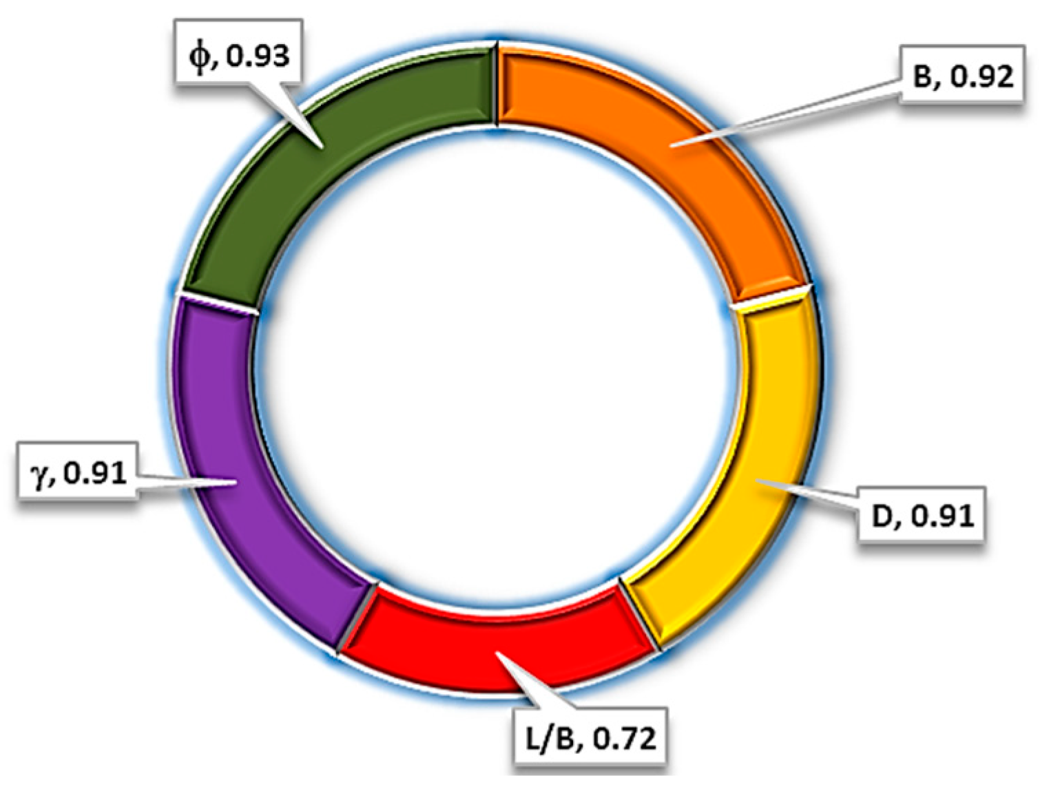
5.5. Sensitivity Analysis
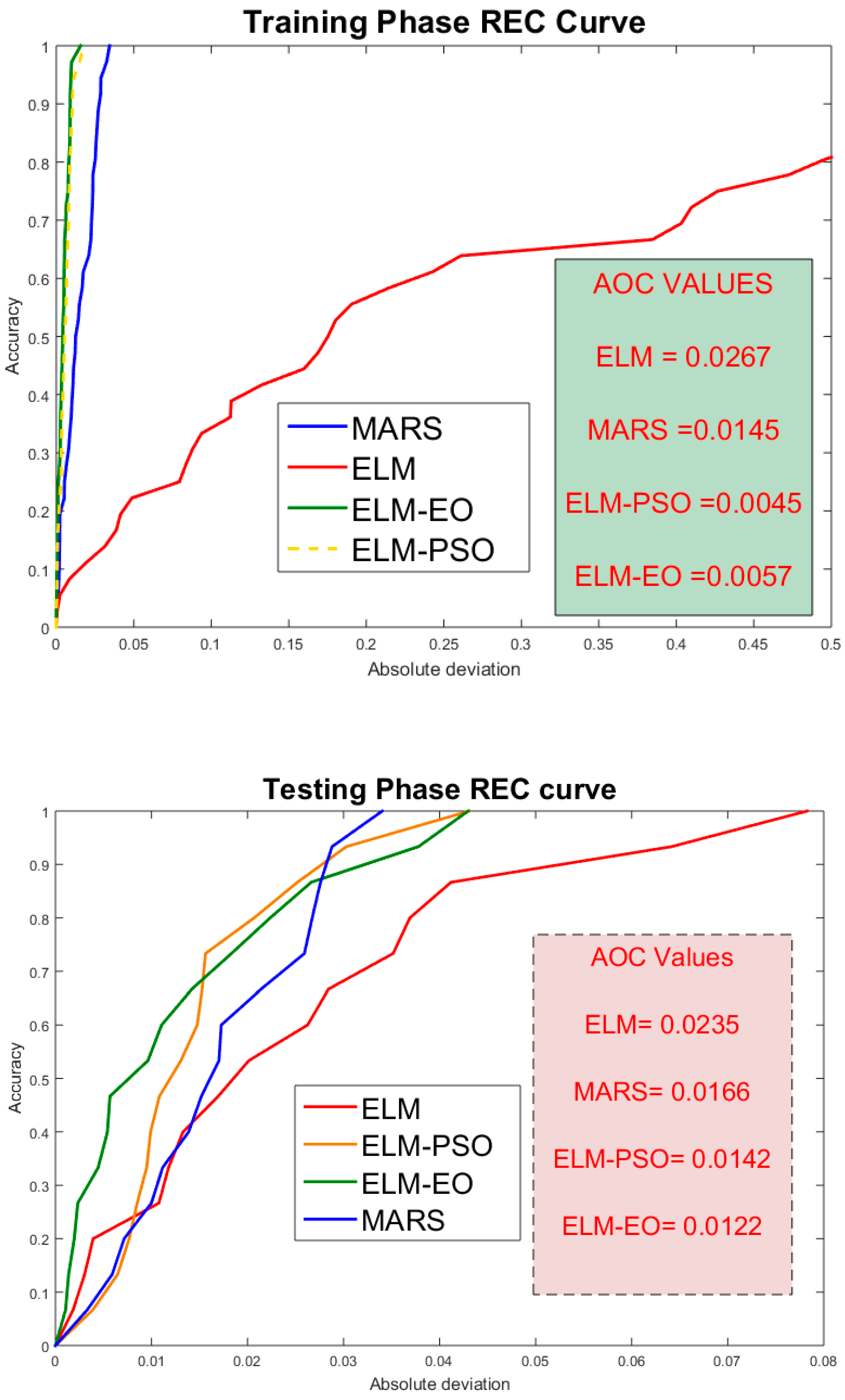
5.6. REC Curves
6. Conclusions
Author Contributions
Funding
Data Availability Statement
Conflicts of Interest
References
- Bowles, J.E. Foundation Analysis and Design, 4th ed.; McGraw-Hill Education: New York, NY, USA, 1988; p. 1004. [Google Scholar]
- Cerato, A.B.; Lutenegger, A.J. Scale Effects of Shallow Foundation Bearing Capacity on Granular Material. J. Geotech. Geoenviron. Eng. 2007, 133, 1192–1202. [Google Scholar] [CrossRef]
- Fukushima, H.I.; Nishimoto, S.; Tomisawa, K. Scale Effect of Spread Foundation Loading Tests Using Various Size Plates; Independent Administrative Institution Civil Engineering Research Institute for Cold Region: Hokkaido, Japan, 2005. [Google Scholar]
- Terzaghi, K. Theoretical Soil Mechanics; John Wiley & Sons, Inc.: Hoboken, NJ, USA, 1943. [Google Scholar]
- Meyerhof, G.G. Some Recent Research on the Bearing Capacity of Foundations. Can. Geotech. J. 1963, 1, 16–26. [Google Scholar] [CrossRef]
- Vesic, A.S. Analysis of Ultimate Loads of Shallow Foundations. ASCE J. Soil Mech. Found. Div. 1973, 99, 45–73. [Google Scholar] [CrossRef]
- Aksoy, H.S.; Gör, M.; İnal, E. A New Design Chart for Estimating Friction Angle between Soil and Pile Materials. Geomech. Eng. 2016, 10, 315. [Google Scholar] [CrossRef]
- Kalinli, A.; Acar, M.C.; Gündüz, Z. New Approaches to Determine the Ultimate Bearing Capacity of Shallow Foundations Based on Artificial Neural Networks and Ant Colony Optimization. Eng. Geol. 2011, 117, 29–38. [Google Scholar] [CrossRef]
- Momeni, E.; Nazir, R.; Jahed Armaghani, D.; Maizir, H. Prediction of Pile Bearing Capacity Using a Hybrid Genetic Algorithm-Based ANN. Meas. J. Int. Meas. Confed. 2014, 57, 122–131. [Google Scholar] [CrossRef]
- Kutter, B.L.; Abghari, A.; Cheney, J.A. Strength Parameters for Bearing Capacity of Sand. J. Geotech. Eng. 1988, 114, 491–498. [Google Scholar] [CrossRef]
- Van Baars, S. Numerical Check of the Meyerhof Bearing Capacity Equation for Shallow Foundations. Innov. Infrastruct. Solut. 2017, 31, 9. [Google Scholar] [CrossRef]
- Rybak, J.; Król, M. Limitations and Risk Related to Static Capacity Testing of Piles-“unfortunate Case” Studies. In Proceedings of the MATEC Web of Conferences, Online, 23 February 2018; Juhásová Šenitková, I., Ed.; EDP Sciences: Les Ulis, France, 2018; Volume 146, p. 02006. [Google Scholar]
- Farooq, F.; Ahmed, W.; Akbar, A.; Aslam, F.; Alyousef, R. Predictive Modeling for Sustainable High-Performance Concrete from Industrial Wastes: A Comparison and Optimization of Models Using Ensemble Learners. J. Clean. Prod. 2021, 292, 126032. [Google Scholar] [CrossRef]
- Farooq, F.; Czarnecki, S.; Niewiadomski, P.; Aslam, F.; Alabduljabbar, H.; Ostrowski, K.A.; Śliwa-Wieczorek, K.; Nowobilski, T.; Malazdrewicz, S. A Comparative Study for the Prediction of the Compressive Strength of Self-Compacting Concrete Modified with Fly Ash. Materials 2021, 14, 4934. [Google Scholar] [CrossRef]
- Javed, M.F.; Amin, M.N.; Shah, M.I.; Khan, K.; Iftikhar, B.; Farooq, F.; Aslam, F.; Alyousef, R.; Alabduljabbar, H. Applications of Gene Expression Programming and Regression Techniques for Estimating Compressive Strength of Bagasse Ash Based Concrete. Crystals 2020, 10, 737. [Google Scholar] [CrossRef]
- Khan, M.A.; Farooq, F.; Javed, M.F.; Zafar, A.; Ostrowski, K.A.; Aslam, F.; Malazdrewicz, S.; Maślak, M. Simulation of Depth of Wear of Eco-Friendly Concrete Using Machine Learning Based Computational Approaches. Materials 2021, 15, 58. [Google Scholar] [CrossRef] [PubMed]
- Song, H.; Ahmad, A.; Farooq, F.; Ostrowski, K.A.; Maślak, M.; Czarnecki, S.; Aslam, F. Predicting the Compressive Strength of Concrete with Fly Ash Admixture Using Machine Learning Algorithms. Constr. Build. Mater. 2021, 308, 125021. [Google Scholar] [CrossRef]
- Ray, R.; Kumar, D.; Samui, P.; Roy, L.B.; Goh, A.T.C.; Zhang, W. Application of Soft Computing Techniques for Shallow Foundation Reliability in Geotechnical Engineering. Geosci. Front. 2021, 12, 375–383. [Google Scholar] [CrossRef]
- Debnath, S.; Sultana, P. Prediction of Settlement of Shallow Foundation on Cohesionless Soil Using Artificial Neural Network. In Proceedings of the 7th Indian Young Geotechnical Engineers Conference; Springer: Singapore, 2022; pp. 477–486. [Google Scholar] [CrossRef]
- Samui, P. Application of Statistical Learning Algorithms to Ultimate Bearing Capacity of Shallow Foundation on Cohesionless Soil. Int. J. Numer. Anal. Methods Geomech. 2012, 36, 100–110. [Google Scholar] [CrossRef]
- Bagińska, M.; Srokosz, P.E. The Optimal ANN Model for Predicting Bearing Capacity of Shallow Foundations Trained on Scarce Data. KSCE J. Civ. Eng. 2018, 23, 130–137. [Google Scholar] [CrossRef] [Green Version]
- Padmini, D.; Ilamparuthi, K.; Sudheer, K.P. Ultimate Bearing Capacity Prediction of Shallow Foundations on Cohesionless Soils Using Neurofuzzy Models. Comput. Geotech. 2008, 35, 33–46. [Google Scholar] [CrossRef]
- Ahmad, M.; Ahmad, F.; Wróblewski, P.; Al-Mansob, R.A.; Olczak, P.; Kamiński, P.; Safdar, M.; Rai, P. Prediction of Ultimate Bearing Capacity of Shallow Foundations on Cohesionless Soils: A Gaussian Process Regression Approach. Appl. Sci. 2021, 11, 10317. [Google Scholar] [CrossRef]
- Huang, G.-B.; Kheong Siew, C.; Zhu, Q.-Y.; Siew, C.-K. Extreme Learning Machine: A New Learning Scheme of Feedforward Neural Networks Sentence Level Sentiment Analysis View Project Neural Networks View Project Extreme Learning Machine: A New Learning Scheme of Feedforward Neural Networks. In Proceedings of the 2004 IEEE International Joint Conference on Neural Networks, Budapest, Hungary, 25–29 July 2004. [Google Scholar] [CrossRef]
- Liu, Z.; Shao, J.; Xu, W.; Chen, H.; Zhang, Y. An Extreme Learning Machine Approach for Slope Stability Evaluation and Prediction. Nat. Hazards 2014, 73, 787–804. [Google Scholar] [CrossRef]
- Samui, P.; Kim, D.; Jagan, J.; Roy, S.S. Determination of Uplift Capacity of Suction Caisson Using Gaussian Process Regression, Minimax Probability Machine Regression and Extreme Learning Machine. Iran. J. Sci. Technol. Trans. Civ. Eng. 2019, 43, 651–657. [Google Scholar] [CrossRef]
- Samui, P. Application of Artificial Intelligence in Geo-Engineering. In Springer Series in Geomechanics and Geoengineering; Springer: Amsterdam, The Netherlands, 2019; pp. 30–44. [Google Scholar] [CrossRef]
- Ghani, S.; Kumari, S.; Choudhary, A.K.; Jha, J.N. Experimental and Computational Response of Strip Footing Resting on Prestressed Geotextile-Reinforced Industrial Waste. Innov. Infrastruct. Solut. 2021, 62, 98. [Google Scholar] [CrossRef]
- Kang, F.; Li, J.-S.; Wang, Y.; Li, J. Extreme Learning Machine-Based Surrogate Model for Analyzing System Reliability of Soil Slopes. Eur. J. Environ. Civ. Eng. 2017, 21, 1341–1362. [Google Scholar] [CrossRef]
- Khaleel, F.; Hameed, M.M.; Khaleel, D.; AlOmar, M.K. Applying an Efficient AI Approach for the Prediction of Bearing Capacity of Shallow Foundations; Springer: Cham, Switzerland, 2022; pp. 310–323. [Google Scholar] [CrossRef]
- Kardani, N.; Bardhan, A.; Samui, P.; Nazem, M.; Zhou, A.; Armaghani, D.J. A Novel Technique Based on the Improved Firefly Algorithm Coupled with Extreme Learning Machine (ELM-IFF) for Predicting the Thermal Conductivity of Soil. Eng. Comput. 2021, 1–20. [Google Scholar] [CrossRef]
- Bardhan, A.; GuhaRay, A.; Gupta, S.; Pradhan, B.; Gokceoglu, C. A Novel Integrated Approach of ELM and Modified Equilibrium Optimizer for Predicting Soil Compression Index of Subgrade Layer of Dedicated Freight Corridor. Transp. Geotech. 2022, 32, 100678. [Google Scholar] [CrossRef]
- Kardani, N.; Bardhan, A.; Roy, B.; Samui, P.; Nazem, M.; Armaghani, D.J.; Zhou, A. A Novel Improved Harris Hawks Optimization Algorithm Coupled with ELM for Predicting Permeability of Tight Carbonates. Eng. Comput. 2021, 1–24. [Google Scholar] [CrossRef]
- Gör, M. Analyzing the Bearing Capacity of Shallow Foundations on Two-Layered Soil Using Two Novel Cosmology-Based Optimization Techniques. Smart Struct. Syst. 2022, 29, 513. [Google Scholar] [CrossRef]
- Moayedi, H.; Gör, M.; Kok Foong, L.; Bahiraei, M. Imperialist Competitive Algorithm Hybridized with Multilayer Perceptron to Predict the Load-Settlement of Square Footing on Layered Soils. Measurement 2021, 172, 108837. [Google Scholar] [CrossRef]
- Jing, Z. Study on Deformation Law of Foundation Pit by Multifractal Detrended Fluctuation Analysis and Extreme Learning Machine Improved by Particle Swarm Optimization. J. Yangtze River Sci. Res. Inst. 2019, 36, 53. [Google Scholar] [CrossRef]
- Li, W.; Li, B.; Guo, H.; Fang, Y.; Qiao, F.; Zhou, S. The Ecg Signal Classification Based on Ensemble Learning of Pso-Elm Algorithm. Neural Netw. World 2020, 30, 265–279. [Google Scholar] [CrossRef]
- Zeng, J.; Roy, B.; Kumar, D.; Mohammed, A.S.; Armaghani, D.J.; Zhou, J.; Mohamad, E.T. Proposing Several Hybrid PSO-Extreme Learning Machine Techniques to Predict TBM Performance. Eng. Comput. 2021, 1, 1–17. [Google Scholar] [CrossRef]
- Chen, F.; Sun, X.; Wei, D.; Tang, Y. Tradeoff Strategy between Exploration and Exploitation for PSO. Proc. 2011 7th Int. Conf. Nat. Comput. ICNC 2011, 3, 1216–1222. [Google Scholar] [CrossRef]
- Grimaldi, E.A.; Grimaccia, F.; Mussetta, M.; Zich, R.E. PSO as an Effective Learning Algorithm for Neural Network Applications. In Proceedings of the ICCEA 2004. 2004 3rd International Conference on Computational Electromagnetics and its Applications, Beijing, China, 1–4 November 2004; pp. 557–560. [Google Scholar] [CrossRef]
- Askarzadeh, A.; Rezazadeh, A. Artificial Bee Swarm Optimization Algorithm for Parameters Identification of Solar Cell Models. Appl. Energy 2013, 102, 943–949. [Google Scholar] [CrossRef]
- Faramarzi, A.; Heidarinejad, M.; Stephens, B.; Mirjalili, S. Equilibrium Optimizer: A Novel Optimization Algorithm. Knowl.-Based Syst. 2020, 191, 105190. [Google Scholar] [CrossRef]
- Kardani, N.; Bardhan, A.; Gupta, S.; Samui, P.; Nazem, M.; Zhang, Y.; Zhou, A. Predicting Permeability of Tight Carbonates Using a Hybrid Machine Learning Approach of Modified Equilibrium Optimizer and Extreme Learning Machine. Acta Geotech. 2021, 17, 1239–1255. [Google Scholar] [CrossRef]
- Samui, P. Determination of Ultimate Capacity of Driven Piles in Cohesionless Soil: A Multivariate Adaptive Regression Spline Approach. Int. J. Numer. Anal. Methods Geomech. 2012, 36, 1434–1439. [Google Scholar] [CrossRef]
- Zhang, W.; Wu, C. Machine Learning Predictive Models for Pile Drivability: An Evaluation of Random Forest Regression and Multivariate Adaptive Regression Splines. In Springer Series in Geomechanics and Geoengineering; Springer: Cham, Switzerland, 2020. [Google Scholar]
- Samui, P.; Kim, D. Least Square Support Vector Machine and Multivariate Adaptive Regression Spline for Modeling Lateral Load Capacity of Piles. Neural Comput. Appl. 2013, 23, 1123–1127. [Google Scholar] [CrossRef]
- Luat, N.V.; Nguyen, V.Q.; Lee, S.; Woo, S.; Lee, K. An Evolutionary Hybrid Optimization of MARS Model in Predicting Settlement of Shallow Foundations on Sandy Soils. Geomech. Eng. 2020, 21, 583–598. [Google Scholar] [CrossRef]
- Dong, J.; Zhu, Y.; Jia, X.; Shao, M.; Han, X.; Qiao, J.; Bai, C.; Tang, X. Nation-Scale Reference Evapotranspiration Estimation by Using Deep Learning and Classical Machine Learning Models in China. J. Hydrol. 2022, 604, 127207. [Google Scholar] [CrossRef]
- Rahgoshay, M.; Feiznia, S.; Arian, M.; Hashemi, S.A.A. Simulation of Daily Suspended Sediment Load Using an Improved Model of Support Vector Machine and Genetic Algorithms and Particle Swarm. Arab. J. Geosci. 2019, 12, 227. [Google Scholar] [CrossRef]
- Zheng, G.; Zhang, W.; Zhou, H.; Yang, P. Multivariate Adaptive Regression Splines Model for Prediction of the Liquefaction-Induced Settlement of Shallow Foundations. Soil Dyn. Earthq. Eng. 2020, 132, 106097. [Google Scholar] [CrossRef]
- Friedman, J.H. Multivariate Adaptive Regression Splines. Ann. Stat. 1991, 19, 1–67. [Google Scholar] [CrossRef]
- Kumar, V.; Himanshu, N.; Burman, A. Rock Slope Analysis with Nonlinear Hoek–Brown Criterion Incorporating Equivalent Mohr–Coulomb Parameters. Geotech. Geol. Eng. 2019, 37, 4741–4757. [Google Scholar] [CrossRef]
- Seifi, A.; Ehteram, M.; Singh, V.P.; Mosavi, A. Modeling and Uncertainty Analysis of Groundwater Level Using Six Evolutionary Optimization Algorithms Hybridized with ANFIS, SVM, and ANN. Sustainability 2020, 12, 4023. [Google Scholar] [CrossRef]
- Eberhart, R.C.; Shi, Y. Comparison between Genetic Algorithms and Particle Swarm Optimization. In Evolutionary Programming VII; Poroto Saravanam, W.N., Waagen, D., Eiben, A.E., Eds.; Springer: Berlin/Heidelberg, Germany, 1998; pp. 611–616. [Google Scholar]
- Shi, Y.; Eberhart, R.C. Empirical Study of Particle Swarm Optimization. In Proceedings of the 1999 Congress on Evolutionary Computation-CEC99 (Cat. No. 99TH8406), Washington, DC, USA, 6–9 July 1999; pp. 1945–1950. [Google Scholar]
- Samui, P.; Sitharam, T.G. Site Characterization Model Using Artificial Neural Network and Kriging. Int. J. Geomech. 2010, 10, 171–180. [Google Scholar] [CrossRef]
- Legates, D.R.; Mccabe, G.J. A Refined Index of Model Performance: A Rejoinder. Int. J. Climatol. 2013, 33, 1053–1056. [Google Scholar] [CrossRef]
- Moriasi, D.N.; Arnold, J.G.; Van Liew, M.W.; Bingner, R.L.; Harmel, R.D.; Veith, T.L. Model Evaluation Guidelines for Systematic Quantification of Accuracy in Watershed Simulations. Trans. ASABE 2007, 50, 885–900. [Google Scholar] [CrossRef]
- Willmott, C.J. On the Evaluation of Model Performance in Physical Geography. In Spatial Statistics and Models; Springer: Cham, Switzerland, 1984. [Google Scholar]
- Kumar, S.; Rai, B.; Biswas, R.; Samui, P.; Kim, D. Prediction of Rapid Chloride Permeability of Self-Compacting Concrete Using Multivariate Adaptive Regression Spline and Minimax Probability Machine Regression. J. Build. Eng. 2020, 32, 101490. [Google Scholar] [CrossRef]
- Biswas, R.; Samui, P.; Rai, B. Determination of Compressive Strength Using Relevance Vector Machine and Emotional Neural Network. Asian J. Civ. Eng. 2019, 20, 1109–1118. [Google Scholar] [CrossRef]
- Biswas, R.; Rai, B.; Samui, P.; Roy, S.S. Estimating Concrete Compressive Strength Using MARS, LSSVM and GP. Eng. J. 2020, 24, 41–52. [Google Scholar] [CrossRef]
- Biswas, R.; Bardhan, A.; Samui, P.; Rai, B.; Nayak, S.; Armaghani, D.J. Efficient Soft Computing Techniques for the Prediction of Compressive Strength of Geopolymer Concrete. Comput. Concr. 2021, 28, 221–232. [Google Scholar] [CrossRef]


| B (m) | D (m) | L/B (-) | γ (KN/m2) | φ (°) | Q (KPa) | |
|---|---|---|---|---|---|---|
| Mean | 0.11 | 0.08 | 3.92 | 16.45 | 38.95 | 192.84 |
| Minimum | 0.06 | 0.03 | 1.00 | 15.70 | 34.00 | 58.50 |
| Maximum | 0.15 | 0.15 | 6.00 | 17.10 | 42.50 | 423.60 |
| Standard Error | 0.01 | 0.01 | 0.35 | 0.07 | 0.44 | 13.18 |
| Standard Deviation | 0.04 | 0.04 | 2.47 | 0.50 | 3.11 | 94.13 |
| Sample Variance | 0.00 | 0.00 | 6.09 | 0.25 | 9.67 | 8860.48 |
| Kurtosis | −1.55 | −0.82 | −1.94 | −1.28 | −1.21 | −0.38 |
| Skewness | −0.03 | 0.61 | −0.37 | −0.22 | −0.45 | 0.65 |
| Range | 0.09 | 0.12 | 5.00 | 1.40 | 8.50 | 365.10 |
| Parameters | MARS-L |
|---|---|
| GCV penalty per knot | 0 |
| Cubic modelling | 0 (No) |
| Self-interactions | 1 (No) |
| Maximum interactions | 2 |
| Prune | 1 (true) |
| No. of in the final model | 15 |
| SL.NO | Basic Function | Equation |
|---|---|---|
| 1 | BF1 | max(0, φ − 0.352) |
| 2 | BF2 | max(0, 0.352 − φ) |
| 3 | BF3 | BF1 × max(0, D − 0.380) |
| 4 | BF4 | Bf1 × max(0, 0.380 − D) |
| 5 | BF5 | max(0, B − 0.379) |
| 6 | BF6 | max(0, 0.379 − B) |
| 7 | BF7 | BF5 × max(0, γ − 0.57) |
| 8 | BF8 | max(0, D − 0.53) |
| 9 | BF9 | max(0, 0.53 − D) |
| Parameters | |||||
|---|---|---|---|---|---|
| ELM | 25 | ||||
| ELM-PSO | 50 | 25 | 100 | −1 | +1 |
| ELM-EO | 50 | 25 | 100 | −1 | +1 |
| Parameters | Ideal Value | Parameters | Ideal Value |
|---|---|---|---|
| VAF | 100 | RMSE | 0 |
| R2 | 1 | WMAPE | 0 |
| PI | 2 | MAE | 0 |
| WI | 1 | MBE | 0 |
| Adj. R2 | 1 | NMBE | 0 |
| NS | 1 | LMI | 0 |
| RSR | 0 | Bias | 1 |
| Model Statistical Parameters | ELM | ELM-EO | ELM-PSO | MARS | ELM | ELM-EO | ELM-PSO | MARS |
|---|---|---|---|---|---|---|---|---|
| Testing Performance | Training Performance | |||||||
| WMAPE | 0.0797 | 0.0306 | 0.0441 | 0.0498 | 0.0543 | 0.0030 | 0.0127 | 0.0396 |
| RMSE | 0.0558 | 0.0170 | 0.0186 | 0.0199 | 0.0248 | 0.0014 | 0.0060 | 0.0180 |
| VAF | 93.921 | 99.3963 | 99.3155 | 99.3155 | 99.1566 | 99.9973 | 99.951 | 99.5517 |
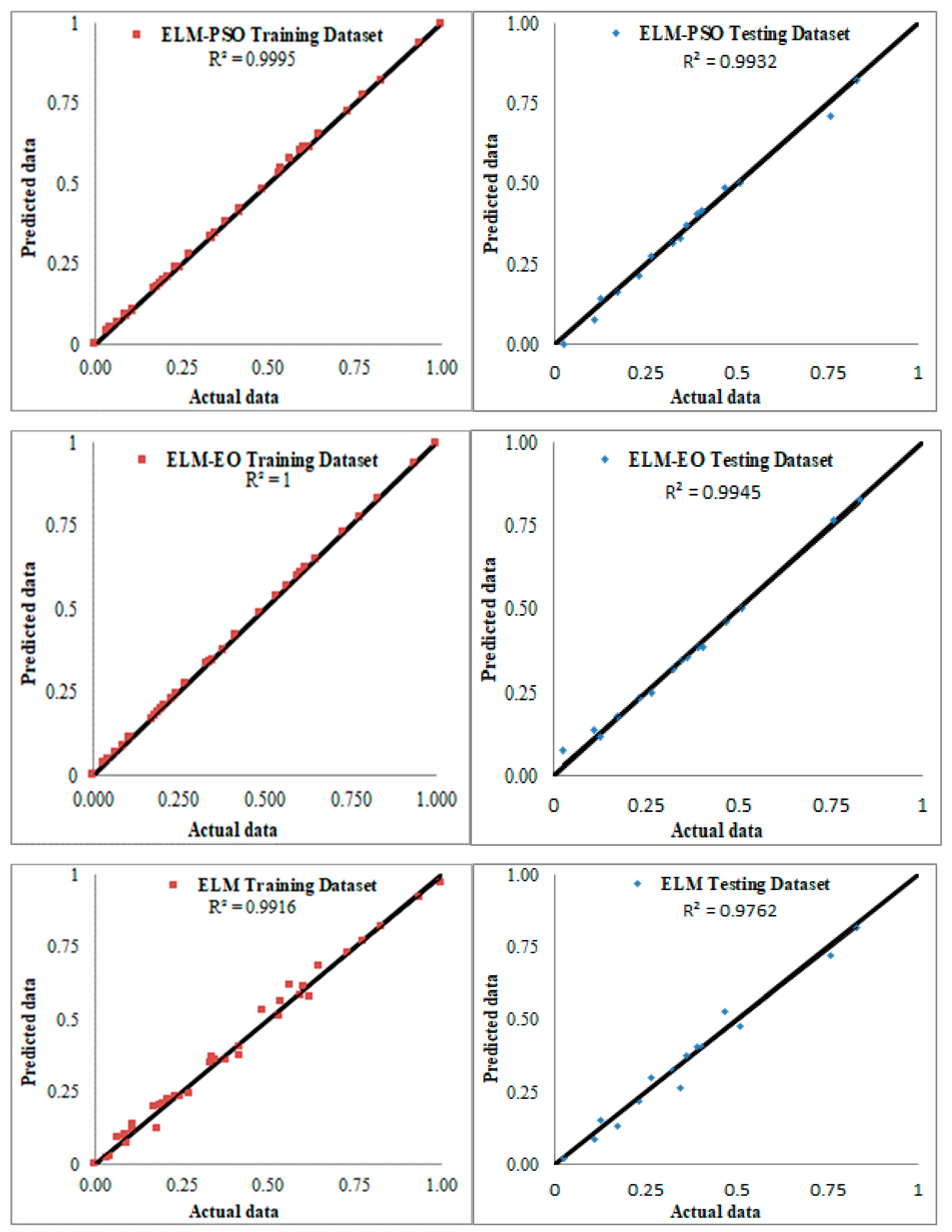
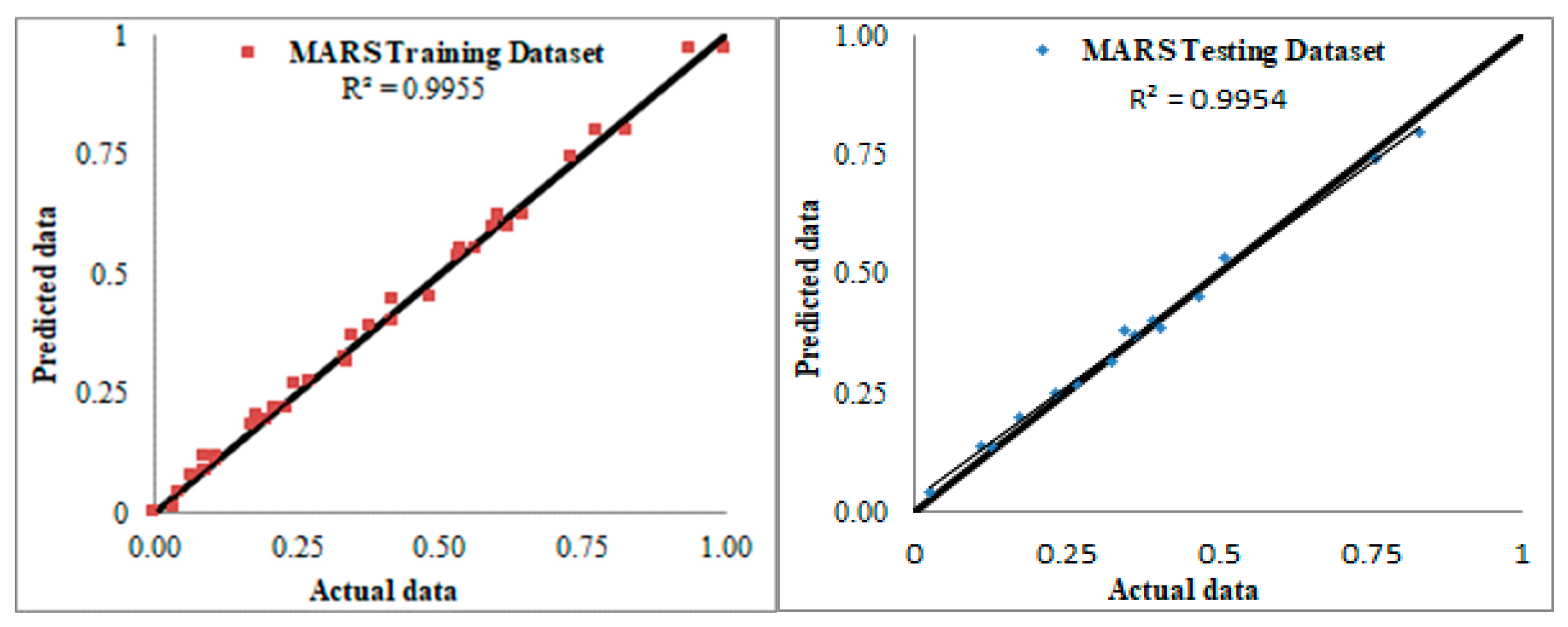
| R2 | 0.9425 | 0.9945 | 0.9932 | 0.9954 | 0.9915 | 0.9999 | 0.9995 | 0.9955 |
| Adj. R2 | 0.9413 | 0.9872 | 0.9840 | 0.9946 | 0.9910 | 0.9999 | 0.9993 | 0.9952 |
| NS | 0.9386 | 0.9938 | 0.9926 | 0.9916 | 0.9915 | 0.9999 | 0.9995 | 0.9955 |
| PI | 1.8247 | 1.9641 | 1.9586 | 1.9673 | 1.9578 | 1.9985 | 1.9930 | 1.9727 |
| RSR | 0.2477 | 0.0785 | 0.0858 | 0.0916 | 0.0919 | 0.0052 | 0.02200 | 0.0669 |
| Bias | 1.0237 | 1.1431 | 0.9178 | 1.0876 | 0.9723 | 0.9731 | 0.9799 | 0.9383 |
| NMBE | −1.0848 | 0.6977 | 1.205 | 1.8913 | 0.1616 | 0.0087 | 0.04750 | 0.1163 |
| WI | 0.9830 | 0.9984 | 0.9982 | 0.9978 | 0.9979 | 0.9999 | 0.9998 | 0.9988 |
| MAE | 0.0398 | 0.01088 | 0.0157 | 0.0177 | 0.0202 | 0.0012 | 0.0048 | 0.0150 |
| MBE | −0.0054 | 0.00248 | −0.0049 | 0.0067 | 0.0006 | 3.24 × 10⁻⁵ | 0.00018 | 0.00044 |
| LMI | 0.7823 | 0.93410 | 0.9052 | 0.8929 | 0.9114 | 0.9950 | 0.9791 | 0.9343 |
| Model Statistical Parameters | ELM | ELM-EO | ELM-PSO | MARS | ELM | ELM-EO | ELM-PSO | MARS | |
|---|---|---|---|---|---|---|---|---|---|
| Testing Performance | Training Performance | ||||||||
| WMAPE | Value | 0.0797 | 0.0306 | 0.0441 | 0.0498 | 0.0543 | 0.0030 | 0.0127 | 0.0396 |
| Score | 1 | 4 | 3 | 2 | 1 | 4 | 3 | 2 | |
| RMSE | Value | 0.0558 | 0.0170 | 0.0186 | 0.0199 | 0.0248 | 0.0014 | 0.0060 | 0.0180 |
| Score | 1 | 4 | 3 | 3 | 1 | 4 | 3 | 3 | |
| VAF | Value | 93.921 | 99.3963 | 99.3155 | 99.3155 | 99.1566 | 99.9973 | 99.951 | 99.5517 |
| Score | 1 | 4 | 3 | 3 | 1 | 4 | 3 | 3 | |
| R2 | Value | 0.9425 | 0.9945 | 0.9932 | 0.9954 | 0.9915 | 0.9999 | 0.9995 | 0.9955 |
| Score | 1 | 3 | 2 | 4 | 1 | 4 | 3 | 2 | |
| Adj. R2 | Value | 0.9413 | 0.9872 | 0.9840 | 0.9946 | 0.9910 | 0.9999 | 0.9993 | 0.9952 |
| Score | 1 | 3 | 2 | 4 | 1 | 4 | 3 | 2 | |
| NS | Value | 0.9386 | 0.9938 | 0.9926 | 0.9916 | 0.9915 | 0.9999 | 0.9995 | 0.9955 |
| Score | 1 | 4 | 3 | 2 | 1 | 4 | 3 | 2 | |
| PI | Value | 1.8247 | 1.9641 | 1.9586 | 1.9673 | 1.9578 | 1.9985 | 1.9930 | 1.9727 |
| Score | 1 | 3 | 2 | 4 | 1 | 4 | 3 | 2 | |
| RSR | Value | 0.2477 | 0.0785 | 0.0858 | 0.0916 | 0.0919 | 0.0052 | 0.02200 | 0.0669 |
| Score | 1 | 4 | 3 | 2 | 1 | 4 | 3 | 2 | |
| Bias | Value | 1.0237 | 1.1431 | 0.9178 | 1.0876 | 0.9723 | 0.9731 | 0.9799 | 0.9383 |
| Score | 2 | 3 | 1 | 3 | 2 | 3 | 4 | 1 | |
| NMBE | Value | −1.0848 | 0.6977 | 12.0509 | 1.8913 | 0.1616 | 0.0087 | 0.04750 | 0.1163 |
| Score | 1 | 2 | 4 | 3 | 4 | 1 | 2 | 3 | |
| WI | Value | 0.9830 | 0.9984 | 0.9982 | 0.9978 | 0.9979 | 0.9999 | 0.9998 | 0.9988 |
| Score | 1 | 4 | 3 | 2 | 1 | 4 | 3 | 2 | |
| MAE | Value | 0.0398 | 0.01088 | 0.0157 | 0.0177 | 0.0202 | 0.0012 | 0.0048 | 0.0150 |
| Score | 1 | 4 | 3 | 2 | 1 | 4 | 3 | 2 | |
| MBE | Value | −0.0054 | 0.00248 | −0.0049 | 0.0067 | 0.0006 | 3.24 × 10⁻⁵ | 0.00018 | 0.00044 |
| Score | 4 | 2 | 3 | 1 | 1 | 4 | 3 | 2 | |
| LMI | Value | 0.7823 | 0.93410 | 0.9052 | 0.8929 | 0.9114 | 0.9950 | 0.9791 | 0.9343 |
| Score | 1 | 4 | 3 | 2 | 1 | 4 | 3 | 2 | |
| Total | 18 | 49 | 38 | 37 | 18 | 52 | 42 | 30 | |
Publisher’s Note: MDPI stays neutral with regard to jurisdictional claims in published maps and institutional affiliations. |
© 2022 by the authors. Licensee MDPI, Basel, Switzerland. This article is an open access article distributed under the terms and conditions of the Creative Commons Attribution (CC BY) license (https://creativecommons.org/licenses/by/4.0/).
Share and Cite
Kumar, M.; Kumar, V.; Biswas, R.; Samui, P.; Kaloop, M.R.; Alzara, M.; Yosri, A.M. Hybrid ELM and MARS-Based Prediction Model for Bearing Capacity of Shallow Foundation. Processes 2022, 10, 1013. https://0-doi-org.brum.beds.ac.uk/10.3390/pr10051013
Kumar M, Kumar V, Biswas R, Samui P, Kaloop MR, Alzara M, Yosri AM. Hybrid ELM and MARS-Based Prediction Model for Bearing Capacity of Shallow Foundation. Processes. 2022; 10(5):1013. https://0-doi-org.brum.beds.ac.uk/10.3390/pr10051013
Chicago/Turabian StyleKumar, Manish, Vinay Kumar, Rahul Biswas, Pijush Samui, Mosbeh R. Kaloop, Majed Alzara, and Ahmed M. Yosri. 2022. "Hybrid ELM and MARS-Based Prediction Model for Bearing Capacity of Shallow Foundation" Processes 10, no. 5: 1013. https://0-doi-org.brum.beds.ac.uk/10.3390/pr10051013