Interval-Valued Pythagorean Fuzzy Similarity Measure-Based Complex Proportional Assessment Method for Waste-to-Energy Technology Selection

Abstract

This study introduces an integrated decision-making methodology to choose the best “waste-to-energy (WTE)” technology for “municipal solid waste (MSW)” treatment under the “interval-valued Pythagorean fuzzy sets (IPFSs)”. In this line, first, a new similarity measure is developed for IPFSs. To show the utility of the developed similarity measure, a comparison is presented with some extant similarity measures. Next, a weighting procedure based on the presented similarity measures is proposed to obtain the criteria weight. Second, an integrated approach called the “interval-valued Pythagorean fuzzy-complex proportional assessment (IPF-COPRAS)” is introduced using the similarity measure, linear programming model and the “complex proportional assessment (COPRAS)” method. Furthermore, a case study of WTE technologies selection for MSW treatment is taken to illustrate the applicability and usefulness of the presented IPF-COPRAS method. The comparative study is made to show the strength and stability of the presented methodology. Based on the results, the most important criteria are “greenhouse gas (GHG)” emissions (P3), microbial inactivation efficacy (P7), air emissions avoidance (P9) and public acceptance (P10) with the weight/significance degrees of 0.200, 0.100, 0.100 and 0.100, respectively. The evaluation results show that the most appropriate WTE technology for MSW treatment is plasma arc gasification (H4) with a maximum utility degree of 0.717 followed by anaerobic digestion (H7) with a utility degree of 0.656 over various considered criteria, which will assist with reducing the amount of waste and GHG emissions and also minimize and maintain the costs of landfills.

1. Introductions

From a global perception, urban regions have been proliferating because of accelerating population growth. Consequently, waste generation is increasing, which is taking into account water and air pollutions, and environmental deterioration. Severe ecological issues arise from several industrial and domestic solid wastes, mainly within urban societies [1,2]. India is fast growing from an agricultural-based country to an industrial and services-based nation. Approximately 31.2% of the population is currently living in urban regions. More than 377 million urban citizens live in 7935 villages/cities [3]. India has diverse climatic and geographic provinces (tropical wet and dry, subtropical humid) and four seasons (winter, summer, rain and autumn). Therefore, the people living in the shared zones have various waste generation and consumption patterns. Nevertheless, no actual process has been analyzed yet to examine provincial and geographical-precise waste generation prototypes for urban areas. Thus, this study relies on the limited information available according to the research accomplished by “Central Pollution Control Board (CPCB)”, New Delhi; “Central Institute of Plastics Engineering and Technology (CIPET)”, Chennai and “Federation of Indian Chambers of Commerce and Industry (FICCI)”, New Delhi [3,4].

The “municipal solid waste (MSW)” is a specific type of waste stemming from households, and it can comprise industrial and commercial wastes. At present, around 2.01 billion metric tons of MSW are generated yearly worldwide. The worldwide annual MSW production rate is expected to grow up to 2.59 “billion metric tons (BMTs)” by 2030 to 3.40 BMTs by 2050 [5,6]. This significant growth in MSW production is recognized as a consequence of diverse aspects, containing economic development, population growth, industrial expansion, urban development and relocation from rural to urban [6,7]. Accompanied by the filling up of waste capacities, the MSW composition is appealing, because it is more heterogeneous and multifaceted due to the expansion of advance economies that are vastly based on user lifestyle [8,9].

The heterogeneity and intricacy of MSW combination are causing excessive difficulty in the sustainable disposal of this enormous quantity of waste that causes several economic damages and shapes severe impacts on the atmosphere and human health [10,11]. It is documented that diverse income level groups produce diverse types of waste compositions and amounts [5,12]. The yearly MSW production growth rate for low to high-income nations has been projected as 2–3% to 3.2–4.5%, respectively [9]. This change among the MSW production growth rates of diverse income groups revealed that the nations with superior purchasing power produce more waste as emerging nations are quickly moving toward industrialization [6]. Regarding the waste collection, high-income nations produce the majority of dry waste, comprising papers, plastics, glasses, metals and others, which is relatively easy to recycle. In contrast, approximately 50% of the MSW production in low-income nations is biological waste, which is more challenging to handle [5]. Worldwide energy requirement has also increased with the multiple increased plight of MSW production and its sustainable management.

Around the world, power generation and transport sectors are two major energy-intensive regions all over the world. The majority of energy requirements in these regions are met by costly fossil fuels [13]. In addition, these “conventional energy resources (CERs)” are quickly diminishing and intimidating energy security worldwide [14,15]. Alternatively, the employment of “renewable energy resources (RESs)” for heat, power, and diverse forms of biofuels generation has reached higher significance in nationwide and worldwide energy plans [12]. Using MSW as an energy source can decrease the severe environmental effects of inappropriate waste management performance and fossil-based electricity power generation [16]. “Waste-to-energy (WTE)” plants can transform this economical and readily accessible RES into useful energy. Consequently, WTE can potentially ensure worldwide energy security by compensating for the dominance of fossil fuels in the global energy region [17]. The word ‘WTE’ describes treating the waste for energy retrieval in heat and electric or other fuels in different states. A variety of WTE procedures are accessible to generate such a different way of end-products from the multifaceted composed feedstock, i.e., “MSW” [12,18].

Assessment of an optimal WTE technology is an intricate “multi-criteria decision-making (MCDM)” procedure that contains various factors, for instance, “waste quality and quantity (WQQ)”, environmental, technological and economic aspects [1,12,19]. The assessment of the most desirable WTE technology recognized saves time and money and helps reduce the negative consequences on the environment [1,19]. Since selecting WTE technology option(s) for the conversion of waste into energy is a complicated decision-making problem, strategic decisions are vital for the efficient assessment and management of these sustainable energy schemes [12,20]. This paper develops an integrated MCDM method that accounts for uncertainty in decision making. In this regard, uncertainties in all steps, which are basically lacking in the preceding literature, were treated in this study. Uncertainty generally occurs in data collection, the data itself, and the evaluation procedure [21]. In this paper, uncertainty in data collection is reduced by conducting the questionnaires between the researchers, experts, and specialists. The interval-values Pythagorean fuzzy sets (IPFSs) are also applied to decrease data uncertainty. Furthermore, an integrated decision-making framework is utilized to address uncertainties related to the evaluation procedure. The combination of different assessment frameworks can help researchers find more accurate outcomes.

To deal with imprecise or uncertain information/data, Zadeh [22] pioneered the concept of “fuzzy sets (FSs)”. Afterwards, Atanassov [23] put forward the idea of “intuitionistic fuzzy sets (IFSs)”, which is related to each object of discourse set not only acquiring a “belongingness degree (BD)” but also “non-belongingness degree (NBD)” such that their sum is less than or equal to one. Consequently, IFSs are proved as a more valuable tool than FSs. The “interval-valued intuitionistic fuzzy sets (IIFSs)” theory was developed by Atanassov and Gargov [24] for treating the ambiguity in data and fuzziness in “decision expert’s (DE’s)” opinions in practical MCDM problems. In the theory of IIFS, both the BD and the NBD of an object are considered and taken in the form of interval values instead of exact numbers. Consequently, there is a substantial requirement to explore more productive and appropriate mathematical approaches utilizing the IIFSs successively to better handle MCDM problems with the high degrees of uncertainty and ambiguity.

Nonetheless, in various actual circumstances, the addition of BD and NBD to an element fulfilled and presented by a DE may be greater than one, whereas their squares addition is $\le 1$. As a result, IFSs fail to tackle such a situation. In order to conquer such situations, Yager [25] commenced the theory of “Pythagorean fuzzy sets (PFSs)” in which the squares sum of BD and NBD is $\le 1$. Therefore, the notion of PFS is considered as a more reliable tool to handle the practical MCDM problems with uncertain information [25]. PFS theory has been explored from several perspectives, including aggregation operators [26,27], decision-making technologies [28,29,30], and information measures [31,32].

Afterwards, the theory of “interval-valued Pythagorean fuzzy sets (IPFSs)” has been introduced by Peng and Yang [33]. As a generalization of PFSs and IIFSs, the IPFSs have wide applications in the discipline of MCDM, such as in emerging sustainable community-based tourism [34] and hospital-based post-acute care assessment [35]. Liang et al. [36] presented the maximizing deviation approach using an IPF-aggregation operator in order to deal with practical MCDM problems. The Bonferroni mean operator [37] and Einstein operator [38] for IPFSs were developed to aggregate the IPFSs for handling the group decision-making problems. In a study, numerous score and accuracy degrees of IPFSs were proposed by Garg [39] for addressing some comparative concerns to solve the MCDM problems. Chen [40] proposed a novel IPF “elimination et choix taduisant la realité (ELECTRE)” method by applying a risk assignment model for solving a financial decision-making problem under an IPFS environment. Peng and Li [41] developed novel IPF operators and established models to solve emergency problems. He et al. [34] designed an IPF information-based model for sustainable community-based tourism. Al-Barakati et al. [42] discussed the work in two folds. Firstly, they reviewed various RESs potential and then proposed an integrated method with the “weighted aggregated sum product assessment (WASPAS)” model and similarity measure for prioritizing the RESs on IPFSs.

Meanwhile, the “complex proportional assessment (COPRAS)” framework, presented by Zavadskas et al. [43], is the MCDM approach, which establishes an outcome and the ratio to the “ideal solution (IS)” and the “anti-ideal solution (AIS)”, and thus, it can be obtained as a compromising model. Recently, the COPRAS approach has been applied under IFSs [44], “picture fuzzy sets (PiFSs)” [45], interval-valued intuitionistic fuzzy sets (IIFSs) [46], “hesitant fuzzy sets (HFSs)” [47], “probabilistic hesitant fuzzy sets (PHFSs)” [48], “Pythagorean fuzzy sets (PFSs)” [49] and “single-valued neutrosophic sets (SVNSs)” [50] to tackle real-life decision-making applications. Furthermore, Roozbahani et al. [51] presented an integrated model by combining “fuzzy sets (FSs)” and a gray COPRAS model for treating the realistic MCDM problem. Mishra et al. [52] developed the idea of “interval-valued hesitant Fermatean fuzzy sets (IVHFFSs)”. Then, they extended the conventional COPRAS methodology to choose the “desalination technology (DT)” for treating the feed water on IVHFFSs. Rani et al. [53] proposed an approach by combining the “criteria interaction through inter-criteria correlation (CRITIC)” and the COPRAS methods to assess and rank the “sustainable community-based tourism (SCBT)” location problem.

Motivation and Novelty

With the rapid growth of the economy, increasing complexity, and society’s continuous progress, MCDM problems have become progressively complex with their noticeable uncertainty and fuzziness of human behavior. Consequently, in the MCDM process, unlike the proper representation of “crisp (precise) numbers (CNs)”, the representation of input parameters in terms of interval values is more appropriate in the recent decision-making settings. Inspired by this notion, the present work is focused on the IPFS environment. The concept of IPFSs is an extension of PFSs [33,34,35]. IPFSs are three-dimensional, and their BD, NBD and “hesitation degree (HD)” are given by an interval within [0, 1]. In the meantime, the only condition is that the squares sum of respective upper bounds of BD and NBD is $\le 1$. On the other hand, to obtain the similarity degree between elements, the measure of similarity is extensively applied information measures in various disciplines and a vital tool in data analysis, decision analysis, medical treatment, and others. As the “similarity measure (SM)” has extensively been implemented in real-life problems, therefore, the SM-based weighting procedure is developed to obtain the weights of criteria. It is observed from the extant research that there is no study to extend the classical COPRAS to the IPF-COPRAS approach to evaluate and prioritize WTE technology for MSW management over various criteria. Thus, in this study, we have developed the IPF-similarity measure-based COPRAS method and implemented it to waste-to-energy technology selection for MSW treatment under IPFSs. Finally, to evaluate the criteria weights, a “linear programming model (LP-model)” is constructed based on similarity measures for IPFSs. The primary contributions stemming from this work are as follows:

-

This study proposes a new IPF similarity measure to evade the shortcomings of existing measures. Furthermore, we utilize it to compute the criteria weights for the waste-to-energy technology selection problem.

-

Corresponding to Liu and Wang [54] for IFSs, we develop a procedure under IPFSs to evaluate the DEs’ weights. In addition, a similarity measure-based LP-model is developed to assess the criteria weights.

-

To illustrate the WTE technology selection for MSW treatment with qualitative and quantitative criteria, an extended COPRAS method is introduced under IPFSs. Subsequently, a problem of waste-to-energy technology assessment is taken to exemplify the usefulness and stability of the proposed ones.

The organization of the paper is discussed as Section 2 elucidates some basic ideas about the IPFSs. Section 3 discusses a novel similarity measure for IPFSs with their properties. Section 4 proposes an IPF-COPRAS methodology based on similarity measures within the IPFSs setting. Section 5 reveals an application of WTE technology selection for the MSW treatment problem and compares the developed approach with existing ones. Finally, concluding remarks are in Section 6.

2. Basic Concepts

In this section, the elementary conceptions of PFSs, IPFSs and IPF similarity measures are discussed.

Definition 1

([25]). A PFS $\overline{\mathrm{A}}$ on a fixed set $\mathsf{\Theta }=\hspace{0.17em}\left\{z_1,\hspace{0.17em}{z}_2,\hspace{0.17em}\dots ,\hspace{0.17em}{z}_n\right\}$ is described as

$$\overline{\mathrm{A}}\hspace{0.17em}=\hspace{0.17em}\left\{\langle z_i,\hspace{0.17em}\overline{\mathrm{A}}\left({\mathsf{\mu }}_{\overline{\mathrm{A}}}(z_i),\hspace{0.17em}{\mathsf{\nu }}_{\overline{\mathrm{A}}}(z_i)\right)\rangle |\hspace{0.17em}{z}_i\hspace{0.17em}\in \hspace{0.17em}\mathsf{\Theta }\right\},$$

where ${\mathsf{\mu }}_{\overline{\mathrm{A}}}\hspace{0.17em}:\hspace{0.17em}\mathsf{\Theta }\hspace{0.17em}\to \hspace{0.17em}\left[0,\hspace{0.17em}1\right]$ and ${\mathsf{\nu }}_{\overline{\mathrm{A}}}\hspace{0.17em}:\hspace{0.17em}\mathsf{\Theta }\hspace{0.17em}\to \hspace{0.17em}\left[0,\hspace{0.17em}1\right]$ exemplify the BD and NBD of an element $z_i\hspace{0.17em}\in \hspace{0.17em}\mathsf{\Theta }$ to $\overline{\mathrm{A}},$ respectively, satisfying $0\hspace{0.17em}\le \hspace{0.17em}{\left({\mathsf{\mu }}_{\overline{\mathrm{A}}}\left(z_i\right)\right)}^2\hspace{0.17em}+\hspace{0.17em}{\left({\mathsf{\nu }}_{\overline{\mathrm{A}}}\left(z_i\right)\right)}^2\hspace{0.17em}\le \hspace{0.17em}1.$ For each $z_i\hspace{0.17em}\in \hspace{0.17em}\mathsf{\Theta },$ the hesitancy degree is defined by ${\mathsf{\pi }}_{\overline{\mathrm{A}}}(z_i)\hspace{0.17em}=\hspace{0.17em}\sqrt{1\hspace{0.17em}-\hspace{0.17em}{\mathsf{\mu }}_{\overline{\mathrm{A}}}^2(z_i)\hspace{0.17em}-\hspace{0.17em}{\mathsf{\nu }}_{\overline{\mathrm{A}}}^2(z_i)\hspace{0.17em}}.$ The notion of “Pythagorean fuzzy number (PFN)” is denoted by $\overline{\mathsf{\alpha }}\hspace{0.17em}=\hspace{0.17em}\left({\mathsf{\mu }}_{\overline{\mathsf{\alpha }}},\hspace{0.17em}{\mathsf{\nu }}_{\overline{\mathsf{\alpha }}}\right)$ which satisfies ${\mathsf{\mu }}_{\overline{\mathsf{\alpha }}},\hspace{0.17em}{\mathsf{\nu }}_{\overline{\mathsf{\alpha }}}\hspace{0.17em}\in \hspace{0.17em}\left[0,\hspace{0.17em}1\right]$ and $0\hspace{0.17em}\le \hspace{0.17em}{\mathsf{\mu }}_{\overline{\mathsf{\alpha }}}^2\hspace{0.17em}+\hspace{0.17em}{\mathsf{\nu }}_{\overline{\mathsf{\alpha }}}^2\hspace{0.17em}\le \hspace{0.17em}1$ [55].

Definition 2

([56]). Consider $\mathsf{\Theta }=\hspace{0.17em}\left\{z_1,\hspace{0.17em}{z}_2,\hspace{0.17em}\dots ,\hspace{0.17em}{z}_n\right\}$ is a fixed set and $Int\left[0,\hspace{0.17em}1\right]$ signifies the collection of all closed subintervals of $\left[0,\hspace{0.17em}1\right].$ Mathematically, an IPFS K in $\mathsf{\Theta }$ is defined by

$$K\hspace{0.17em}=\hspace{0.17em}\left\{\langle z_i,\hspace{0.17em}\left[{\mathsf{\mu }}_K^{-}(z_i),\hspace{0.17em}{\mathsf{\mu }}_K^{+}(z_i)\right],\hspace{0.17em}\left[{\mathsf{\nu }}_K^{-}(z_i),\hspace{0.17em}{\mathsf{\nu }}_K^{+}(z_i)\right]\rangle \hspace{0.17em}:\hspace{0.17em}{z}_i\hspace{0.17em}\in \hspace{0.17em}\mathsf{\Theta }\right\},$$

where $0\hspace{0.17em}\le {\mathsf{\mu }}_K^{-}(z_i)\hspace{0.17em}\le \hspace{0.17em}{\mathsf{\mu }}_K^{+}(z_i)\hspace{0.17em}\le 1,$ $0\hspace{0.17em}\le {\mathsf{\nu }}_K^{-}(z_i)\hspace{0.17em}\le \hspace{0.17em}{\mathsf{\nu }}_K^{+}(z_i)\hspace{0.17em}\le 1$ and $0\le {\left({\mathsf{\mu }}_K^{+}(z_i)\hspace{0.17em}\right)}^2+\hspace{0.17em}\hspace{0.17em}{\left({\mathsf{\nu }}_K^{+}(z_i)\right)}^2\le 1.$ Here, ${\mathsf{\mu }}_K(z_i)\hspace{0.17em}=\hspace{0.17em}\left[{\mathsf{\mu }}_K^{-}(z_i),\hspace{0.17em}{\mathsf{\mu }}_K^{+}(z_i)\right]$ and ${\mathsf{\nu }}_K(z_i)\hspace{0.17em}=\hspace{0.17em}\left[{\mathsf{\nu }}_K^{-}(z_i),\hspace{0.17em}{\mathsf{\nu }}_K^{+}(z_i)\right]$ define the BD and NBD of an element $z_i$ to $\mathsf{\Theta },$ respectively. There are two special cases of IPFS (see Figure 1). (i) An IPFS is changed to an IIFS if $0\le {\mathsf{\mu }}_K^{+}(z_i)+\hspace{0.17em}\hspace{0.17em}{\mathsf{\nu }}_K^{+}(z_i)\hspace{0.17em}\le 1.$ (ii) An IPFS is transformed to a PFS if ${\mathsf{\mu }}_K^{-}\left(z_i\right)\hspace{0.17em}=\hspace{0.17em}{\mathsf{\mu }}_K^{+}\left(z_i\right)$ and ${\mathsf{\nu }}_K^{-}\left(z_i\right)\hspace{0.17em}=\hspace{0.17em}{\mathsf{\nu }}_K^{+}\left(z_i\right).$

The function ${\mathsf{\pi }}_K\left(z_i\right)\hspace{0.17em}=\hspace{0.17em}\left[{\mathsf{\pi }}_K^{-}(z_i),\hspace{0.17em}{\mathsf{\pi }}_K^{+}(z_i)\right]$ represents the hesitancy degree of $z_i$ to K, wherein ${\mathsf{\pi }}_K^{-}(z_i)\hspace{0.17em}=\hspace{0.17em}\sqrt{1\hspace{0.17em}-\hspace{0.17em}{\left({\mathsf{\mu }}_K^{+}(z_i)\right)}^2\hspace{0.17em}-\hspace{0.17em}{\left({\mathsf{\nu }}_K^{+}(z_i)\right)}^2\hspace{0.17em}}$ and ${\mathsf{\pi }}_K^{+}(z_i)\hspace{0.17em}=\hspace{0.17em}\sqrt{1\hspace{0.17em}-\hspace{0.17em}{\left({\mathsf{\mu }}_K^{-}(z_i)\right)}^2\hspace{0.17em}-\hspace{0.17em}{\left({\mathsf{\nu }}_K^{-}(z_i)\right)}^2\hspace{0.17em}}\hspace{0.17em}.$ For simplicity, the “interval-valued Pythagorean fuzzy number (IPFN)” is denoted by $\mathsf{\alpha }\hspace{0.17em}=\hspace{0.17em}\left(\left[{\mathsf{\mu }}_{\mathsf{\alpha }}^{-},\hspace{0.17em}{\mathsf{\mu }}_{\mathsf{\alpha }}^{+}\right],\hspace{0.17em}\left[{\mathsf{\nu }}_{\mathsf{\alpha }}^{-},\hspace{0.17em}{\mathsf{\nu }}_{\mathsf{\alpha }}^{+}\right]\right)$, which fulfills $0\le {\left(b_{\mathsf{\alpha }}^{+}\right)}^2+\hspace{0.17em}\hspace{0.17em}{\left(n_{\mathsf{\alpha }}^{+}\right)}^2\le 1.$

Definition 3

([56]). Let ${\mathsf{\alpha }}_1\hspace{0.17em}=\hspace{0.17em}\hspace{0.17em}\left(\left[{\mathsf{\mu }}_{{\mathsf{\alpha }}_1}^{-},\hspace{0.17em}{\mathsf{\mu }}_{{\mathsf{\alpha }}_1}^{+}\right],\hspace{0.17em}\left[{\mathsf{\nu }}_{{\mathsf{\alpha }}_1}^{-},\hspace{0.17em}{\mathsf{\nu }}_{{\mathsf{\alpha }}_1}^{+}\right]\right),$ ${\mathsf{\alpha }}_2\hspace{0.17em}=\hspace{0.17em}\hspace{0.17em}\left(\left[{\mathsf{\mu }}_{{\mathsf{\alpha }}_2}^{-},\hspace{0.17em}{\mathsf{\mu }}_{{\mathsf{\alpha }}_2}^{+}\right],\hspace{0.17em}\left[{\mathsf{\nu }}_{{\mathsf{\alpha }}_2}^{-},\hspace{0.17em}{\mathsf{\nu }}_{{\mathsf{\alpha }}_2}^{+}\right]\right)$ and ${\mathsf{\alpha }}_3\hspace{0.17em}=\hspace{0.17em}\hspace{0.17em}\left(\left[{\mathsf{\mu }}_{{\mathsf{\alpha }}_3}^{-},\hspace{0.17em}{\mathsf{\mu }}_{{\mathsf{\alpha }}_3}^{+}\right],\hspace{0.17em}\left[{\mathsf{\nu }}_{{\mathsf{\alpha }}_3}^{-},\hspace{0.17em}{\mathsf{\nu }}_{{\mathsf{\alpha }}_3}^{+}\right]\right)$ be the IPFNs. Then, some fundamental operations are defined as

$$\begin{array}{c}{\mathsf{\alpha }}_1\hspace{0.17em}\oplus \hspace{0.17em}{\mathsf{\alpha }}_2\hspace{0.17em}=\hspace{0.17em}\left([\sqrt{{\left({\mathsf{\mu }}_{{\mathsf{\alpha }}_1}^{-}\right)}^2\hspace{0.17em}+\hspace{0.17em}{\left({\mathsf{\mu }}_{{\mathsf{\alpha }}_2}^{-}\right)}^2\hspace{0.17em}-\hspace{0.17em}{\left({\mathsf{\mu }}_{{\mathsf{\alpha }}_1}^{-}\right)}^2\hspace{0.17em}{\left({\mathsf{\mu }}_{{\mathsf{\alpha }}_2}^{-}\right)}^2},\hspace{0.17em}\sqrt{{\left({\mathsf{\mu }}_{{\mathsf{\alpha }}_1}^{+}\right)}^2\hspace{0.17em}+\hspace{0.17em}{\left({\mathsf{\mu }}_{{\mathsf{\alpha }}_2}^{+}\right)}^2\hspace{0.17em}-\hspace{0.17em}{\left({\mathsf{\mu }}_{{\mathsf{\alpha }}_1}^{+}\right)}^2\hspace{0.17em}{\left({\mathsf{\mu }}_{{\mathsf{\alpha }}_2}^{+}\right)}^2}],\hspace{0.17em}\hspace{0.17em}\left[{\mathsf{\nu }}_{{\mathsf{\alpha }}_1}^{-}\hspace{0.17em}{\mathsf{\nu }}_{{\mathsf{\alpha }}_2}^{-},\hspace{0.17em}\hspace{0.17em}{\mathsf{\nu }}_{{\mathsf{\alpha }}_1}^{+}\hspace{0.17em}{\mathsf{\nu }}_{{\mathsf{\alpha }}_2}^{+}\right]\right),\hfill \\ {\mathsf{\alpha }}_1\hspace{0.17em}\otimes \hspace{0.17em}{\mathsf{\alpha }}_2\hspace{0.17em}=\hspace{0.17em}\left(\left[{\mathsf{\mu }}_{{\mathsf{\alpha }}_1}^{-}\hspace{0.17em}{\mathsf{\mu }}_{{\mathsf{\alpha }}_2}^{-},\hspace{0.17em}\hspace{0.17em}{\mathsf{\mu }}_{{\mathsf{\alpha }}_1}^{+}\hspace{0.17em}{\mathsf{\mu }}_{{\mathsf{\alpha }}_2}^{+}\right],\hspace{0.17em}[\sqrt{{\left({\mathsf{\nu }}_{{\mathsf{\alpha }}_1}^{-}\right)}^2\hspace{0.17em}+\hspace{0.17em}{\left({\mathsf{\nu }}_{{\mathsf{\alpha }}_2}^{-}\right)}^2\hspace{0.17em}-\hspace{0.17em}{\left({\mathsf{\nu }}_{{\mathsf{\alpha }}_1}^{-}\right)}^2\hspace{0.17em}{\left({\mathsf{\nu }}_{{\mathsf{\alpha }}_2}^{-}\right)}^2},\hspace{0.17em}\hspace{0.17em}\sqrt{{\left({\mathsf{\nu }}_{{\mathsf{\alpha }}_1}^{+}\right)}^2\hspace{0.17em}+\hspace{0.17em}{\left({\mathsf{\nu }}_{{\mathsf{\alpha }}_2}^{+}\right)}^2\hspace{0.17em}-\hspace{0.17em}{\left({\mathsf{\nu }}_{{\mathsf{\alpha }}_1}^{+}\right)}^2\hspace{0.17em}{\left({\mathsf{\nu }}_{{\mathsf{\alpha }}_2}^{+}\right)}^2}]\right),\hfill \\ \lambda \hspace{0.17em}{\mathsf{\alpha }}_1\hspace{0.17em}=\hspace{0.17em}\left([\sqrt{1-\hspace{0.17em}{\left(1\hspace{0.17em}-\hspace{0.17em}{\left({\mathsf{\mu }}_{{\mathsf{\alpha }}_1}^{-}\right)}^2\right)}^{\lambda }},\hspace{0.17em}\sqrt{1-\hspace{0.17em}{\left(1\hspace{0.17em}-\hspace{0.17em}{\left({\mathsf{\mu }}_{{\mathsf{\alpha }}_1}^{+}\right)}^2\right)}^{\lambda }}],\hspace{0.17em}\left[{\left({\mathsf{\nu }}_{{\mathsf{\alpha }}_1}^{-}\right)}^{\lambda },\hspace{0.17em}\hspace{0.17em}{\left({\mathsf{\nu }}_{{\mathsf{\alpha }}_1}^{+}\right)}^{\lambda }\right]\right),\hfill \\ {\left({\mathsf{\alpha }}_1\right)}^{\lambda }\hspace{0.17em}=\hspace{0.17em}\left(\left[{\left({\mathsf{\mu }}_{{\mathsf{\alpha }}_1}^{-}\right)}^{\lambda },\hspace{0.17em}{\left({\mathsf{\mu }}_{{\mathsf{\alpha }}_1}^{-}\right)}^{\lambda }\right],\hspace{0.17em}\hspace{0.17em}[\sqrt{1-\hspace{0.17em}{\left(1\hspace{0.17em}-\hspace{0.17em}{\left({\mathsf{\nu }}_{{\mathsf{\alpha }}_1}^{-}\right)}^2\right)}^{\lambda }},\hspace{0.17em}\sqrt{1-\hspace{0.17em}{\left(1\hspace{0.17em}-\hspace{0.17em}{\left({\mathsf{\nu }}_{{\mathsf{\alpha }}_1}^{+}\right)}^2\right)}^{\lambda }}]\right),{\left({\mathsf{\alpha }}_1\right)}^c\hspace{0.17em}=\hspace{0.17em}\left(\left[{\mathsf{\nu }}_{{\mathsf{\alpha }}_1}^{-},\hspace{0.17em}{\mathsf{\nu }}_{{\mathsf{\alpha }}_1}^{+}\right],\hspace{0.17em}\left[{\mathsf{\mu }}_{{\mathsf{\alpha }}_1}^{-},\hspace{0.17em}{\mathsf{\mu }}_{{\mathsf{\alpha }}_1}^{+}\right]\right).\hfill \end{array}$$

Definition 4

([33]). Assume $\mathsf{\alpha }\hspace{0.17em}=\hspace{0.17em}\hspace{0.17em}\left(\left[{\mathsf{\mu }}_{\mathsf{\alpha }}^{-},\hspace{0.17em}{\mathsf{\mu }}_{\mathsf{\alpha }}^{+}\right],\hspace{0.17em}\left[{\mathsf{\nu }}_{\mathsf{\alpha }}^{-},\hspace{0.17em}{\mathsf{\nu }}_{\mathsf{\alpha }}^{+}\right]\right)$ is an IPFN. Then

$$\mathbb{S}\left(\mathsf{\alpha }\right)=\frac{1}{2}\left({\left({\mathsf{\mu }}_{\mathsf{\alpha }}^{-}\right)}^2\hspace{0.17em}+\hspace{0.17em}{\left({\mathsf{\mu }}_{\mathsf{\alpha }}^{+}\right)}^2\hspace{0.17em}-\hspace{0.17em}{\left({\mathsf{\nu }}_{\mathsf{\alpha }}^{-}\right)}^2-{\left({\mathsf{\nu }}_{\mathsf{\alpha }}^{+}\right)}^2\right)$$

and

$$\hslash \left(\mathsf{\alpha }\right)=\frac{1}{2}\left({\left({\mathsf{\mu }}_{\mathsf{\alpha }}^{-}\right)}^2\hspace{0.17em}+\hspace{0.17em}{\left({\mathsf{\mu }}_{\mathsf{\alpha }}^{+}\right)}^2\hspace{0.17em}+\hspace{0.17em}{\left({\mathsf{\nu }}_{\mathsf{\alpha }}^{-}\right)}^2+{\left({\mathsf{\nu }}_{\mathsf{\alpha }}^{+}\right)}^2\right),$$

(1)

are given as the score and accuracy values of an IPFN $\mathsf{\alpha },$ respectively, where $\mathbb{S}\left(\mathsf{\alpha }\right)\in \left[-1,1\right]$ and $\hslash \left(\mathsf{\alpha }\right)\in \left[0,1\right]$.

For any two IPFNs, the ranking principle using the score and accuracy functions and are defined by

(a)

If $\mathbb{S}\left({\mathsf{\alpha }}_1\right)<\mathbb{S}\left({\mathsf{\alpha }}_2\right)$ then ${\mathsf{\alpha }}_1\hspace{0.17em}<{\mathsf{\alpha }}_2,$

(b)

If $\mathbb{S}\left({\mathsf{\alpha }}_1\right)>\mathbb{S}\left({\mathsf{\alpha }}_2\right)$ then ${\mathsf{\alpha }}_1\hspace{0.17em}<{\mathsf{\alpha }}_2,$

(c)

If $\mathbb{S}\left({\mathsf{\alpha }}_1\right)=\mathbb{S}\left({\mathsf{\alpha }}_2\right)$ then

• If $\hslash \left({\mathsf{\alpha }}_1\right)<\hslash \left({\mathsf{\alpha }}_2\right)$ then ${\mathsf{\alpha }}_1\hspace{0.17em}<{\mathsf{\alpha }}_2,$
• If $\hslash \left({\mathsf{\alpha }}_1\right)>\hslash \left({\mathsf{\alpha }}_2\right)$ then ${\mathsf{\alpha }}_1\hspace{0.17em}<{\mathsf{\alpha }}_2,$
• If $\hslash \left({\mathsf{\alpha }}_1\right)=\hslash \left({\mathsf{\alpha }}_2\right)$ then ${\mathsf{\alpha }}_1\hspace{0.17em}<{\mathsf{\alpha }}_2.$

Definition 5

([57]). Consider $\mathsf{\alpha }\hspace{0.17em}=\hspace{0.17em}\hspace{0.17em}\left(\left[{\mathsf{\mu }}_{\mathsf{\alpha }}^{-},\hspace{0.17em}{\mathsf{\mu }}_{\mathsf{\alpha }}^{+}\right],\hspace{0.17em}\left[{\mathsf{\nu }}_{\mathsf{\alpha }}^{-},\hspace{0.17em}{\mathsf{\nu }}_{\mathsf{\alpha }}^{+}\right]\right)$ being an IPFN. Then

$${\mathbb{S}}^{*}\left(\mathsf{\alpha }\right)=\frac{\left({\left({\mathsf{\mu }}_{\mathsf{\alpha }}^{-}\right)}^2-\hspace{0.17em}{\left({\mathsf{\nu }}_{\mathsf{\alpha }}^{-}\right)}^2\hspace{0.17em}\right)\left(1+\sqrt{1-{\left({\mathsf{\mu }}_{\mathsf{\alpha }}^{-}\right)}^2-\hspace{0.17em}{\left({\mathsf{\nu }}_{\mathsf{\alpha }}^{-}\right)}^2}\right)+\hspace{0.17em}\left({\left({\mathsf{\mu }}_{\mathsf{\alpha }}^{+}\right)}^2\hspace{0.17em}-{\left({\mathsf{\nu }}_{\mathsf{\alpha }}^{+}\right)}^2\right)\left(1+\sqrt{1-{\left({\mathsf{\mu }}_{\mathsf{\alpha }}^{+}\right)}^2-\hspace{0.17em}{\left({\mathsf{\nu }}_{\mathsf{\alpha }}^{+}\right)}^2}\right)}{2},$$

(2)

is said to be an improved score function of IPFN $\mathsf{\alpha }$ and ${\mathbb{S}}^{*}\left(\mathsf{\alpha }\right)\in \left[-1,1\right].$

Definition 6

([56]). Let ${\mathsf{\alpha }}_1\hspace{0.17em}=\hspace{0.17em}\left(\left[{\mathsf{\mu }}_{{\mathsf{\alpha }}_1}^{-},\hspace{0.17em}{\mathsf{\mu }}_{{\mathsf{\alpha }}_1}^{+}\right],\hspace{0.17em}\left[{\mathsf{\nu }}_{{\mathsf{\alpha }}_1}^{-},\hspace{0.17em}{\mathsf{\nu }}_{{\mathsf{\alpha }}_1}^{+}\right]\right)$ and ${\mathsf{\alpha }}_2\hspace{0.17em}=\hspace{0.17em}\left(\left[{\mathsf{\mu }}_{{\mathsf{\alpha }}_2}^{-},\hspace{0.17em}{\mathsf{\mu }}_{{\mathsf{\alpha }}_2}^{+}\right],\hspace{0.17em}\left[{\mathsf{\nu }}_{{\mathsf{\alpha }}_2}^{-},\hspace{0.17em}{\mathsf{\nu }}_{{\mathsf{\alpha }}_2}^{+}\right]\right)$ be two IPFNs. Then, the following relations are satisfied:

${\mathsf{\alpha }}_1\hspace{0.17em}=\hspace{0.17em}{\mathsf{\alpha }}_2$ if and only if ${\mathsf{\mu }}_{{\mathsf{\alpha }}_1}^{-}=\hspace{0.17em}{\mathsf{\mu }}_{{\mathsf{\alpha }}_2}^{-},$ ${\mathsf{\mu }}_{{\mathsf{\alpha }}_1}^{+}=\hspace{0.17em}{\mathsf{\mu }}_{{\mathsf{\alpha }}_2}^{+},$ ${\mathsf{\nu }}_{{\mathsf{\alpha }}_1}^{-}=\hspace{0.17em}{\mathsf{\nu }}_{{\mathsf{\alpha }}_2}^{-}$ and ${\mathsf{\nu }}_{{\mathsf{\alpha }}_1}^{+}=\hspace{0.17em}{\mathsf{\nu }}_{{\mathsf{\alpha }}_2}^{+}.$

${\mathsf{\alpha }}_1\hspace{0.17em}\prec \hspace{0.17em}\hspace{0.17em}{\mathsf{\alpha }}_2$ if and only if ${\mathsf{\mu }}_{{\mathsf{\alpha }}_1}^{-}\le \hspace{0.17em}\hspace{0.17em}{\mathsf{\mu }}_{{\mathsf{\alpha }}_2}^{-},$ ${\mathsf{\mu }}_{{\mathsf{\alpha }}_1}^{+}\le \hspace{0.17em}{\mathsf{\mu }}_{{\mathsf{\alpha }}_2}^{+},$ ${\mathsf{\nu }}_{{\mathsf{\alpha }}_1}^{-}\ge \hspace{0.17em}\hspace{0.17em}{\mathsf{\nu }}_{{\mathsf{\alpha }}_2}^{-}$ and ${\mathsf{\nu }}_{{\mathsf{\alpha }}_1}^{+}\ge \hspace{0.17em}\hspace{0.17em}{\mathsf{\nu }}_{{\mathsf{\alpha }}_2}^{+}.$

Definition 7

([56]). An IPF similarity measure $S\hspace{0.17em}:\hspace{0.17em}IPFSs\left(\mathsf{\Theta }\right)\hspace{0.17em}\times \hspace{0.17em}IPFSs\left(\mathsf{\Theta }\right)\to ℝ$ is a real-valued mapping that fulfills the given axioms as

(S1)$0\le S\left(K,\hspace{0.17em}L\right)\hspace{0.17em}\le 1\hspace{0.17em};\hspace{0.17em}\hspace{0.17em}\forall \hspace{0.17em}K,\hspace{0.17em}L\in IPFSs\left(\mathsf{\Theta }\right),$

(S2)$S\left(K,\hspace{0.17em}L\right)=1$if and only if$K=L\hspace{0.17em};\hspace{0.17em}\hspace{0.17em}\hspace{0.17em}\forall \hspace{0.17em}K,\hspace{0.17em}L\in IPFSs\left(\mathsf{\Theta }\right),$

(S3)$S\left(K,\hspace{0.17em}L\right)=S\left(L,\hspace{0.17em}K\right)\hspace{0.17em};\hspace{0.17em}\forall \hspace{0.17em}K,\hspace{0.17em}L\in IPFSs\left(\mathsf{\Theta }\right),$

(S4)$S\left(K,\hspace{0.17em}{K}^c\right)=0$if and only if$\mathrm{A}$is a crisp set,

(S5) If$K\subseteq \hspace{0.17em}L\subseteq \hspace{0.17em}M,$then$S\left(K,\hspace{0.17em}M\right)\le S\left(K,\hspace{0.17em}L\right)$and$S\left(K,\hspace{0.17em}M\right)\le S\left(L,\hspace{0.17em}M\right)\hspace{0.17em};$$\forall \hspace{0.17em}K,\hspace{0.17em}L,\hspace{0.17em}M\in IPFSs\left(\mathsf{\Theta }\right).$

3. Proposed Similarity Measure for IPFSs

The “Similarity Measure (SM)” is a very significant aspect for assessing the uncertain information. In FS theory, the concept of similarity measure describes the closeness degree between two FSs. Firstly, Zhang [56] initiated the concept of “Pythagorean Fuzzy SM (PF-SM)” and employed it to cope with the practical applications. Peng et al. [58] extended novel entropy, distance and similarity measures to solve the problems that arise in image segmentation and disease diagnosis. Later on, many research efforts have been made in the context of PF-SMs [31,59,60,61,62]. Further, Biswas and Sarkar [63] proposed a point operator based IPF-SMs using a weighted Minkowski distance of IPFNs and “IPF point operators (IPFPOs)” [33]. Peng and Li [41] developed novel similarity, distance and entropy measures for IPFSs and utilized them to discuss the “Weighted Discrimination-Based Approximation (WDBA)” model. Rani and Mishra [64] proposed a “combined compromise solution (CoCoSo)” model with the similarity measure on the “single-valued neutrosophic sets (SVNSs)”, and then, they applied it to treat the “waste electrical and electronics equipment (WEEE)” recycling partner selection problem. Mishra et al. [65] introduced the similarity measure-based “additive ratio assessment (ARAS)” model on SVNSs for assessing and prioritizing the sustainable “electric vehicle charging station (EVCS)” sites. Ünver et al. [66] developed various similarity measures using the Choquet integral for “spherical fuzzy sets (SFSs)”. They also performed these measures in pattern recognition problems to observe a comparative assessment of the proposed ones with some existing similarity measures.

In the current section, we propose new SM for IPFSs and further apply it in the development of the COPRAS method within the IPFSs setting.

Let $K,L\hspace{0.17em}\in IPFSs(\mathsf{\Theta }).$ Then, a new “interval-valued Pythagorean fuzzy similarity measure (IPF-SM)” is defined as

$$S_1(K,\hspace{0.17em}L)=1-\frac{1-\exp \left[-\frac{1}{4n}{\displaystyle \sum _{i=1}^n\left(\begin{array}{l}\left|{\mathsf{\mu }}_K^{-2}\left(z_i\right)\hspace{0.17em}-\hspace{0.17em}{\mathsf{\mu }}_L^{-2}\left(z_i\right)\right|+\left|{\mathsf{\mu }}_K^{+2}\left(z_i\right)\hspace{0.17em}-\hspace{0.17em}{\mathsf{\mu }}_L^{+2}\left(z_i\right)\right|\hspace{0.17em}\hspace{0.17em}\\ \hspace{0.17em}+\left|{\mathsf{\nu }}_K^{-2}\left(z_i\right)\hspace{0.17em}-\hspace{0.17em}{\mathsf{\nu }}_L^{-2}\left(z_i\right)\right|+\left|{\mathsf{\nu }}_K^{+2}\left(z_i\right)\hspace{0.17em}-\hspace{0.17em}{\mathsf{\nu }}_L^{+2}\left(z_i\right)\right|\\ \hspace{0.17em}\hspace{0.17em}\hspace{0.17em}+\left|{\mathsf{\pi }}_K^{-2}\left(z_i\right)\hspace{0.17em}-\hspace{0.17em}{\mathsf{\pi }}_L^{-2}\left(z_i\right)\right|+\left|{\mathsf{\pi }}_K^{+2}\left(z_i\right)\hspace{0.17em}-\hspace{0.17em}{\mathsf{\pi }}_L^{+2}\left(z_i\right)\right|\end{array}\right)}\right]}{1-\exp (-1)}.$$

(3)

Lemma 1.

If$g\left(\gamma \right)=1-\frac{1-\exp \left(-\gamma \right)}{1-\exp \left(-1\right)},$then$\underset{\gamma \in \left[0,\hspace{0.17em}n\right]}{\max }g\left(\gamma \right)=g\left(0\right)=1$and$\underset{\gamma \in \left[0,\hspace{0.17em}n\right]}{\min }g\left(\gamma \right)=g\left(n\right)=0.$

Proof. 

Since $g^{\prime }\left(\gamma \right)=-\frac{\exp \left(-\gamma \right)}{1-\exp \left(-1\right)}<0,\hspace{0.17em}\hspace{0.17em}\forall \hspace{0.17em}\gamma \in \left[0,\hspace{0.17em}\hspace{0.17em}n\right],$ therefore, $g\left(\gamma \right)$ is decreasing in $[0,\hspace{0.17em}n].$ □

Theorem 1.

The measure$S_1(K,\hspace{0.17em}L),$defined in Equation (3), is a valid IPF-similarity measure.

Proof. 

To prove this, we have to validate the axioms (S1)–(S5) of Definition 7.

(S1). For $K,L\hspace{0.17em}\in IPFSs\left(\mathsf{\Theta }\right),$

$$\gamma \hspace{0.17em}=\hspace{0.17em}\frac{1}{4n}{\displaystyle \sum _{i=1}^n\left(\begin{array}{l}\left|{\mathsf{\mu }}_K^{-2}\left(z_i\right)\hspace{0.17em}-\hspace{0.17em}{\mathsf{\mu }}_L^{-2}\left(z_i\right)\right|+\left|{\mathsf{\mu }}_K^{+2}\left(z_i\right)\hspace{0.17em}-\hspace{0.17em}{\mathsf{\mu }}_L^{+2}\left(z_i\right)\right|\hspace{0.17em}\hspace{0.17em}+\left|{\mathsf{\nu }}_K^{-2}\left(z_i\right)\hspace{0.17em}-\hspace{0.17em}{\mathsf{\nu }}_L^{-2}\left(z_i\right)\right|\\ +\left|{\mathsf{\nu }}_K^{+2}\left(z_i\right)\hspace{0.17em}-\hspace{0.17em}{\mathsf{\nu }}_L^{+2}\left(z_i\right)\right|+\left|{\mathsf{\pi }}_K^{-2}\left(z_i\right)\hspace{0.17em}-\hspace{0.17em}{\mathsf{\pi }}_L^{-2}\left(z_i\right)\right|+\left|{\mathsf{\pi }}_K^{+2}\left(z_i\right)\hspace{0.17em}-\hspace{0.17em}{\mathsf{\pi }}_L^{+2}\left(z_i\right)\right|\end{array}\right)}.$$

Since $\mathsf{\beta }\hspace{0.17em}\in \hspace{0.17em}\left[0,\hspace{0.17em}n\right],$ thus, $S_1\left(K,\hspace{0.17em}L\right)\hspace{0.17em}=\hspace{0.17em}g\left(\gamma \right).$ From Lemma 1, we obtain $0\hspace{0.17em}\le \hspace{0.17em}Si{m}_1\left(K,\hspace{0.17em}L\right)\hspace{0.17em}\le \hspace{0.17em}1.$

(S2). From Equation (3), if $K\hspace{0.17em}=\hspace{0.17em}L,$ then $S_1\left(K,\hspace{0.17em}L\right)\hspace{0.17em}=1.$ Conversely, let $S_1\left(K,\hspace{0.17em}L\right)\hspace{0.17em}=1.$

Conversely, let $S_1\left(K,\hspace{0.17em}L\right)\hspace{0.17em}=1.$ Then, from Equation (3), we obtain

$$1-\frac{1-\exp \left[-\frac{1}{4n}{\displaystyle \sum _{i=1}^n\left(\begin{array}{l}\left|{\mathsf{\mu }}_K^{-2}\left(z_i\right)\hspace{0.17em}-\hspace{0.17em}{\mathsf{\mu }}_L^{-2}\left(z_i\right)\right|+\left|{\mathsf{\mu }}_K^{+2}\left(z_i\right)\hspace{0.17em}-\hspace{0.17em}{\mathsf{\mu }}_L^{+2}\left(z_i\right)\right|\hspace{0.17em}\hspace{0.17em}\\ \hspace{0.17em}+\left|{\mathsf{\nu }}_K^{-2}\left(z_i\right)\hspace{0.17em}-\hspace{0.17em}{\mathsf{\nu }}_L^{-2}\left(z_i\right)\right|+\left|{\mathsf{\nu }}_K^{+2}\left(z_i\right)\hspace{0.17em}-\hspace{0.17em}{\mathsf{\nu }}_L^{+2}\left(z_i\right)\right|\\ \hspace{0.17em}\hspace{0.17em}\hspace{0.17em}+\left|{\mathsf{\pi }}_K^{-2}\left(z_i\right)\hspace{0.17em}-\hspace{0.17em}{\mathsf{\pi }}_L^{-2}\left(z_i\right)\right|+\left|{\mathsf{\pi }}_K^{+2}\left(z_i\right)\hspace{0.17em}-\hspace{0.17em}{\mathsf{\pi }}_L^{+2}\left(z_i\right)\right|\end{array}\right)}\right]}{1-\exp (-1)}=1,\hspace{0.17em}\hspace{0.17em}\forall \hspace{0.17em}{z}_i\hspace{0.17em}\in \hspace{0.17em}\mathsf{\Theta }.$$

It implies that

$$\left(\begin{array}{l}\left|{\mathsf{\mu }}_K^{-2}\left(z_i\right)\hspace{0.17em}-\hspace{0.17em}{\mathsf{\mu }}_L^{-2}\left(z_i\right)\right|+\left|{\mathsf{\mu }}_K^{+2}\left(z_i\right)\hspace{0.17em}-\hspace{0.17em}{\mathsf{\mu }}_L^{+2}\left(z_i\right)\right|\hspace{0.17em}\hspace{0.17em}+\left|{\mathsf{\nu }}_K^{-2}\left(z_i\right)\hspace{0.17em}-\hspace{0.17em}{\mathsf{\nu }}_L^{-2}\left(z_i\right)\right|\\ +\left|{\mathsf{\nu }}_K^{+2}\left(z_i\right)\hspace{0.17em}-\hspace{0.17em}{\mathsf{\nu }}_L^{+2}\left(z_i\right)\right|+\left|{\mathsf{\pi }}_K^{-2}\left(z_i\right)\hspace{0.17em}-\hspace{0.17em}{\mathsf{\pi }}_L^{-2}\left(z_i\right)\right|+\left|{\mathsf{\pi }}_K^{+2}\left(z_i\right)\hspace{0.17em}-\hspace{0.17em}{\mathsf{\pi }}_L^{+2}\left(z_i\right)\right|\end{array}\right)=\hspace{0.17em}0.$$

Thus, ${\mathsf{\mu }}_K^{-}\left(z_i\right)=\hspace{0.17em}{\mathsf{\mu }}_L^{-}\left(z_i\right),{\mathsf{\mu }}_K^{+}\left(z_i\right)=\hspace{0.17em}{\mathsf{\mu }}_L^{+}\left(z_i\right),\hspace{0.17em}{\mathsf{\nu }}_K^{-}\left(z_i\right)=\hspace{0.17em}{\mathsf{\nu }}_L^{-}\left(z_i\right),{\mathsf{\nu }}_K^{+}\left(z_i\right)=\hspace{0.17em}{\mathsf{\nu }}_L^{+}\left(z_i\right).$

Hence, $K\hspace{0.17em}=\hspace{0.17em}L.$

(S3)–(S4). Both axioms are straightforward from Equation (3).

(S5). Let $K\hspace{0.17em}\subseteq \hspace{0.17em}L\hspace{0.17em}\subseteq \hspace{0.17em}M,$ then ${\mathsf{\mu }}_K^{-2}\left(z_i\right)\hspace{0.17em}\le \hspace{0.17em}{\mathsf{\mu }}_L^{-2}\left(z_i\right)\hspace{0.17em}\le \hspace{0.17em}{\mathsf{\mu }}_M^{-2}\left(z_i\right),$ ${\mathsf{\mu }}_K^{+2}\left(z_i\right)\hspace{0.17em}\le \hspace{0.17em}{\mathsf{\mu }}_L^{+2}\left(z_i\right)\hspace{0.17em}\le \hspace{0.17em}{\mathsf{\mu }}_M^{+2}\left(z_i\right),$ ${\mathsf{\nu }}_K^{-2}\left(z_i\right)\hspace{0.17em}\ge \hspace{0.17em}{\mathsf{\nu }}_L^{-2}\left(z_i\right)\hspace{0.17em}\ge \hspace{0.17em}{\mathsf{\nu }}_M^{-2}\left(z_i\right),\hspace{0.17em}$ and ${\mathsf{\nu }}_K^{+2}\left(z_i\right)\hspace{0.17em}\ge \hspace{0.17em}{\mathsf{\nu }}_L^{+2}\left(z_i\right)\hspace{0.17em}\ge \hspace{0.17em}{\mathsf{\nu }}_M^{+2}\left(z_i\right),\hspace{0.17em}\forall \hspace{0.17em}{z}_i\hspace{0.17em}\in \hspace{0.17em}\mathsf{\Theta }.$

Then,

$${\gamma }_1\hspace{0.17em}=\hspace{0.17em}\frac{1}{4n}{\displaystyle \sum _{i=1}^n\left(\begin{array}{l}\left|{\mathsf{\mu }}_K^{-2}\left(z_i\right)\hspace{0.17em}-\hspace{0.17em}{\mathsf{\mu }}_L^{-2}\left(z_i\right)\right|+\left|{\mathsf{\mu }}_K^{+2}\left(z_i\right)\hspace{0.17em}-\hspace{0.17em}{\mathsf{\mu }}_L^{+2}\left(z_i\right)\right|\hspace{0.17em}\hspace{0.17em}+\left|{\mathsf{\nu }}_K^{-2}\left(z_i\right)\hspace{0.17em}-\hspace{0.17em}{\mathsf{\nu }}_L^{-2}\left(z_i\right)\right|\\ +\left|{\mathsf{\nu }}_K^{+2}\left(z_i\right)\hspace{0.17em}-\hspace{0.17em}{\mathsf{\nu }}_L^{+2}\left(z_i\right)\right|+\left|{\mathsf{\pi }}_K^{-2}\left(z_i\right)\hspace{0.17em}-\hspace{0.17em}{\mathsf{\pi }}_L^{-2}\left(z_i\right)\right|+\left|{\mathsf{\pi }}_K^{+2}\left(z_i\right)\hspace{0.17em}-\hspace{0.17em}{\mathsf{\pi }}_L^{+2}\left(z_i\right)\right|\end{array}\right)}$$

$$\le \hspace{0.17em}{\gamma }_2\hspace{0.17em}=\hspace{0.17em}\frac{1}{4n}{\displaystyle \sum _{i=1}^n\left(\begin{array}{l}\left|{\mathsf{\mu }}_K^{-2}\left(z_i\right)\hspace{0.17em}-\hspace{0.17em}{\mathsf{\mu }}_M^{-2}\left(z_i\right)\right|+\left|{\mathsf{\mu }}_K^{+2}\left(z_i\right)\hspace{0.17em}-\hspace{0.17em}{\mathsf{\mu }}_M^{+2}\left(z_i\right)\right|\hspace{0.17em}\hspace{0.17em}+\left|{\mathsf{\nu }}_K^{-2}\left(z_i\right)\hspace{0.17em}-\hspace{0.17em}{\mathsf{\nu }}_M^{-2}\left(z_i\right)\right|\\ +\left|{\mathsf{\nu }}_K^{+2}\left(z_i\right)\hspace{0.17em}-\hspace{0.17em}{\mathsf{\nu }}_M^{+2}\left(z_i\right)\right|+\left|{\mathsf{\pi }}_K^{-2}\left(z_i\right)\hspace{0.17em}-\hspace{0.17em}{\mathsf{\pi }}_M^{-2}\left(z_i\right)\right|+\left|{\mathsf{\pi }}_K^{+2}\left(z_i\right)\hspace{0.17em}-\hspace{0.17em}{\mathsf{\pi }}_M^{+2}\left(z_i\right)\right|\end{array}\right),}\forall \hspace{0.17em}{z}_i\hspace{0.17em}\in \hspace{0.17em}\mathsf{\Theta }.$$

Therefore, by Lemma 1, we obtain $S_1\left(K,\hspace{0.17em}L\right)\hspace{0.17em}=\hspace{0.17em}g\left({\gamma }_1\right)\ge \hspace{0.17em}\hspace{0.17em}g\left({\gamma }_2\right)\hspace{0.17em}=\hspace{0.17em}{S}_1\left(K,\hspace{0.17em}M\right).$ Similarly, we can verify that $S_1\left(L,\hspace{0.17em}M\right)\hspace{0.17em}\ge \hspace{0.17em}{S}_1\left(K,\hspace{0.17em}M\right).$ [Proved] □

Moreover, a new IPF-SM is discussed using the association of $S_1\left(K,\hspace{0.17em}L\right)$ and a lattice. In general, a lattice of a non-empty set is a hierarchical system generated by the “partial order sets (POSETs)”. In a lattice, each pair of elements must contain a supremum and an infimum. Now, let $K,L\hspace{0.17em}\in IPFSs(\mathsf{\Theta }).$ Then, the proposed IPF similarity measure is presented as

$$S_2\left(K,\hspace{0.17em}L\right)=\sqrt{S_1\left(K,\hspace{0.17em}{P}_{KL}\right)\times S_1\left(L,P_{KL}\right)}, \mathrm{where} P_{KL}=K\cup \hspace{0.17em}L.$$

(4)

Theorem 2.

The measure$S_2(K,\hspace{0.17em}L),$defined in Equation (4), is a valid IPF similarity measure.

Proof. (S1).

It is straightforward, so that we have omitted the proof.

(S2). Consider $K,\hspace{0.17em}L\in IPFSs\left(\mathsf{\Theta }\right)$ and $K=\hspace{0.17em}L.$ Given that $P_{KL}=K\hspace{0.17em}\cup L,$ this implies that $K=L=P_{KL}$ and so, $S_1\left(K,\hspace{0.17em}L\right)$ fulfills the axiom (S₂). Thus, $S_2\left(K,\hspace{0.17em}L\right)=1.$ Conversely, let $S_2\left(K,\hspace{0.17em}L\right)=1,$ that means that $S_1(K,P_{KL})=$$S_1(L,P_{KL})=1,$ where $P_{KL}=K\hspace{0.17em}\cup L$ and $S_1(K,\hspace{0.17em}L)$ satisfies (S₂). Thus, $K=\hspace{0.17em}L=P_{KL}.$ Hence, measure $S_2(K,\hspace{0.17em}L)$ satisfies (S₂).

(S₃)–(S₄): Both are straightforward from Equation (4).

(S₅): Suppose $K,\hspace{0.17em}L,M\in IPFSs\left(\mathsf{\Theta }\right)$ and $K\subseteq L\subseteq M.$ Then. $K\cup L=L,$ $K\cup M=M$ and $L\cup M=M.$

Now,

$$S_2(K,\hspace{0.17em}M)=\sqrt{S_1\left(K,\hspace{0.17em}{P}_{KM}\right)\times S_1\left(M,\hspace{0.17em}{P}_{KM}\right)}.$$

It implies that

$$S_2\left(K,\hspace{0.17em}M\right)=\sqrt{S_1\left(K,\hspace{0.17em}M\right)\times S_1\left(M,\hspace{0.17em}M\right)}.$$

Thus,

$$S_2\left(K,\hspace{0.17em}M\right)=\sqrt{S_1\left(K,\hspace{0.17em}M\right)}.$$

(5)

Similarly, we can verify that

$$S_2(K,\hspace{0.17em}L)=\sqrt{S_1\left(K,\hspace{0.17em}L\right)}.$$

(6)

Since $S_1\left(K,\hspace{0.17em}M\right)$ holds (S₅), i.e., $S_1\left(K,\hspace{0.17em}L\right)\ge S_1\left(K,\hspace{0.17em}M\right).$ Consequently, from Equation (5) and Equation (6), we obtain $S_2\left(K,\hspace{0.17em}L\right)\ge S_2\left(K,\hspace{0.17em}M\right).$ In a similar line, we can show that $S_2\left(L,\hspace{0.17em}M\right)\ge \hspace{0.17em}{S}_2\left(K,\hspace{0.17em}M\right).$ [Proved] □

Comparison with Existing SMs

Here, a comparative study between the introduced IPF-SM $S_2\left(K,L\right)$ and the existing measures [56,67] has been discussed to explore the benefits of the introduced IPF-SM in the form of distance measure. The extant SMs based on the combination of the Hausdorff, Euclidean, and Hamming distances on IPFNs have been illustrated as follows:

$$\begin{array}{c}\hfill S_H\left(K,\hspace{0.17em}L\right)=1-D_H\left(K,\hspace{0.17em}L\right)=1-\frac{1}{4}(\left|{\mathsf{\mu }}_K^{-}\left(z_i\right)-\hspace{0.17em}{\mathsf{\mu }}_L^{-}\left(z_i\right)\right|+\left|{\mathsf{\mu }}_K^{+}\left(z_i\right)-\hspace{0.17em}{\mathsf{\mu }}_L^{+}\left(z_i\right)\right|\hfill \\ \hfill +\left|{\mathsf{\nu }}_K^{-}\left(z_i\right)-{\mathsf{\nu }}_L^{-}\left(z_i\right)\right|+\left|{\mathsf{\nu }}_K^{+}\left(z_i\right)-\hspace{0.17em}{\mathsf{\nu }}_L^{+}\left(z_i\right)\right|).\hfill \end{array}$$

(7)

$$S_E\left(K,\hspace{0.17em}L\right)=1-D_E\left(K,\hspace{0.17em}L\right)=1-\sqrt{\frac{1}{4}\left(\begin{array}{l}{\left({\mathsf{\mu }}_K^{-}\left(z_i\right)-{\mathsf{\mu }}_L^{-}\left(z_i\right)\right)}^2+{\left({\mathsf{\mu }}_K^{+}\left(z_i\right)-{\mathsf{\mu }}_L^{+}\left(z_i\right)\right)}^2\\ \hspace{0.17em}\hspace{0.17em}\hspace{0.17em}+{\left({\mathsf{\nu }}_K^{-}\left(z_i\right)-{\mathsf{\nu }}_L^{-}\left(z_i\right)\right)}^2+{\left({\mathsf{\nu }}_K^{+}\left(z_i\right)-{\mathsf{\nu }}_L^{+}\left(z_i\right)\right)}^2\end{array}\right)}.$$

(8)

$$S_{HH}\left(K,\hspace{0.17em}L\right)=1-D_{HH}\left(K,\hspace{0.17em}L\right)=1-\max \left(\begin{array}{l}\left|{\mathsf{\mu }}_K^{-}\left(z_i\right)-{\mathsf{\mu }}_L^{-}\left(z_i\right)\right|,\hspace{0.17em}\left|{\mathsf{\mu }}_K^{+}\left(z_i\right)-{\mathsf{\mu }}_L^{+}\left(z_i\right)\right|,\\ \hspace{0.17em}\hspace{0.17em}\hspace{0.17em}\hspace{0.17em}\left|{\mathsf{\nu }}_K^{-}\left(z_i\right)-{\mathsf{\nu }}_L^{-}\left(z_i\right)\right|,\hspace{0.17em}\left|{\mathsf{\nu }}_K^{+}\left(z_i\right)-{\mathsf{\nu }}_L^{+}\left(z_i\right)\right|\end{array}\right).$$

(9)

$$S_{HE}\left(K,\hspace{0.17em}L\right)=1-D_{HE}\left(K,\hspace{0.17em}L\right)=1-\sqrt{\max \left(\begin{array}{l}{\left({\mathsf{\mu }}_K^{-}\left(z_i\right)-{\mathsf{\mu }}_L^{-}\left(z_i\right)\right)}^2,\hspace{0.17em}{\left({\mathsf{\mu }}_K^{+}\left(z_i\right)-{\mathsf{\mu }}_L^{+}\left(z_i\right)\right)}^2,\\ \hspace{0.17em}\hspace{0.17em}\hspace{0.17em}\hspace{0.17em}{\left({\mathsf{\nu }}_K^{-}\left(z_i\right)-{\mathsf{\nu }}_L^{-}\left(z_i\right)\right)}^2,\hspace{0.17em}{\left({\mathsf{\nu }}_K^{+}\left(z_i\right)-{\mathsf{\nu }}_L^{+}\left(z_i\right)\right)}^2\end{array}\right)}.$$

(10)

$$S_Z\left(K,\hspace{0.17em}L\right)=1-D_Z\left(K,\hspace{0.17em}L\right)=1-\frac{1}{4}\left(\begin{array}{l}\left|{\left({\mathsf{\mu }}_K^{-}\left(z_i\right)\right)}^2-{\left({\mathsf{\mu }}_L^{-}\left(z_i\right)\right)}^2\right|+\left|{\left({\mathsf{\mu }}_K^{+}\left(z_i\right)\right)}^2-{\left({\mathsf{\mu }}_L^{+}\left(z_i\right)\right)}^2\right|\\ \hspace{0.17em}+\left|{\left({\mathsf{\nu }}_K^{-}\left(z_i\right)\right)}^2-{\left({\mathsf{\nu }}_L^{-}\left(z_i\right)\right)}^2\right|+\left|{\left({\mathsf{\nu }}_K^{+}\left(z_i\right)\right)}^2-{\left({\mathsf{\nu }}_L^{+}\left(z_i\right)\right)}^2\right|\\ \hspace{0.17em}\hspace{0.17em}\hspace{0.17em}+\left|{\left({\mathsf{\pi }}_K^{-}\left(z_i\right)\right)}^2-{\left({\mathsf{\pi }}_L^{-}\left(z_i\right)\right)}^2\right|+\left|{\left({\mathsf{\pi }}_K^{+}\left(z_i\right)\right)}^2-{\left({\mathsf{\pi }}_L^{+}\left(z_i\right)\right)}^2\right|\end{array}\right).$$

(11)

Here,

Table 1. Comparison results of introduced IPF-SM with extant ones.

K L	${\mathit{S}}_{\mathit{H}}\left(\mathit{K},\hspace{0.17em}\mathit{L}\right)$	${\mathit{S}}_{\mathit{E}}\left(\mathit{K},\hspace{0.17em}\mathit{L}\right)$	${\mathit{S}}_{\mathit{H}\mathit{H}}\left(\mathit{K},\hspace{0.17em}\mathit{L}\right)$	${\mathit{S}}_{\mathit{H}\mathit{E}}\left(\mathit{K},\hspace{0.17em}\mathit{L}\right)$	${\mathit{S}}_{\mathit{Z}}\left(\mathit{K},\hspace{0.17em}\mathit{L}\right)$	${\mathit{S}}_2\left(\mathit{K},\hspace{0.17em}\mathit{L}\right)$
$\left(\left[0.26,0.36\right],\left[0.26,0.36\right]\right)$$\left(\left[0.36,0.46\right],\left[0.36,0.46\right]\right)$	0.9	0.9	0.9	0.9	0.8854	0.9119
$\left(\left[0.26,0.36\right],\left[0.36,0.46\right]\right)$$\left(\left[0.36,0.46\right],\left[0.26,0.36\right]\right)$	0.9	0.9	0.9	0.9	0.928	0.9425
$\left(\left[1.00,1.00\right],\left[0.00,0.00\right]\right)$$\left(\left[0.00,0.00\right],\left[1.00,1.00\right]\right)$	0.0	0.0	0.0	0.0	0.0	0.0
$\left(\left[1.00,1.00\right],\left[0.00,0.00\right]\right)$$\left(\left[0.00,0.00\right],\left[0.00,0.00\right]\right)$	0.5	0.2929	0.0	0.0	0.0	0.3133
$\left(\left[0.50,0.0\right],\left[0.50,0.50\right]\right)$$\left(\left[0.00,0.00\right],\left[0.00,0.00\right]\right)$	0.5	0.5	0.5	0.5	0.6036	0.7155
$\left(\left[0.36,0.46\right],\left[0.16,0.26\right]\right)$$\left(\left[0.46,0.56\right],\left[0.26,0.36\right]\right)$	0.9	0.9	0.9	0.9	0.8848	0.9113
$\left(\left[0.36,0.46\right],\left[0.16,0.26\right]\right)$$\left(\left[0.46,0.56\right],\left[0.16,0.26\right]\right)$	0.95	0.9293	0.9	0.9	0.9270	0.9427

Note: “Bold” symbolizes an unreasonable result that means counter-intuitive cases.

demonstrates a comparison of similarity measures for IPFSs with different counter-intuitive examples.

Existing SMs ($S_H,S_E,S_{HH}$ and $S_{HE}$) fall short of discriminating positive change from negative change. For example, $S_H\left(K,\hspace{0.17em}L\right)=0.9$ and $S_H\left(K_1,L_1\right)=0.9;$ $S_E\left(K,\hspace{0.17em}L\right)=0.9$ and $S_E\left(K_1,L_1\right)=0.9;$ $S_{HH}\left(K,\hspace{0.17em}L\right)=0.9;$ $S_{HH}\left(K_1,L_1\right)=0.9;$ $S_{HE}\left(K,\hspace{0.17em}L\right)=0.9;$ and $S_{HH}\left(K_1,\hspace{0.17em}{L}_1\right)=0.9;$ when K = ([0.26, 0.36], [0.26, 0.36]); L = ([0.36, 0.46], [0.36, 0.46]); K₁ = ([0.26, 0.36], [0.36; 0.46]) and L₁ = ([0.36, 0.46], [0.26, 0.36]). Alternatively, the proposed SM S₂ can efficiently discriminate positive from negative changes on account of $S_2\left(K,\hspace{0.17em}L\right)=0.9119$ and $S_2\left(K_1,\hspace{0.17em}{L}_1\right)=0.9425$ in the same example. Additionally, another counter-intuitive case will occur in which $S_H\left(K,\hspace{0.17em}L\right)=0.5$ and $S_H\left(K_1,\hspace{0.17em}{L}_1\right)=0.5$ are equal if K = ([1.0, 1.0], [0.0, 0.0]); L = ([0.0, 0.0], [0.0, 0.0]). For IPFNs, K₁ = ([0.5, 0.5], [0.5, 0.5]); L₁ = ([0.0, 0.0], [0.0, 0.0]), the SMs $S_Z\left(K,\hspace{0.17em}L\right)=0.6036,$ $S_2\left(K,\hspace{0.17em}L\right)=0.7155$ and remaining extant SMs have counter-intuitive cases because other extant SMs do not contain the third parameter of IPFNs that means hesitancy or indeterminacy degree. Furthermore, the existing ones except the above have presented different outcomes, which are more rational.

Next, it is evident that the postulate of IPF-SM (S4) is not fulfilled by $S_{HH},S_{HE}$ and $S_Z.$ It means that only the third row for all SMs is equal to 0.

Finally, the last counter-intuitive state occurs when K = ([0.36, 0.46], [0.16, 0.26]); L = ([0.46, 0.56], [0.26, 0.36]); K₁ = ([0.46, 0.56], [0.16, 0.26]), since IPFNs K, L and K₁ are ranked as $K_1\succ L\succ K$ by Definition 5. Moreover, $S_{HH}\left(K,\hspace{0.17em}L\right)=S_{HH}\left(L,K_1\right)=0.9$ and $S_{HE}\left(K,\hspace{0.17em}L\right)=$$S_{HE}\left(L,K_1\right)=0.9$ are not reasonable. Hence, to investigate all the counter-intuitive cases, the SMs $S_Z\left(K,\hspace{0.17em}L\right)$ and $S_2$ is only one that validates the mentioned counter-intuitive cases, as depicted in Table 1.

4. IPF-COPRAS Methodology for MCDM Problems

In this section, the traditional COPRAS method is generalized to handle the MCDM problems on IPFSs, in which the criterion weight information is entirely unknown. The notions and operational laws of the IPFNs, IPF-SM and score function are employed to develop the IPF-COPRAS approach. The procedure of the IPF-COPRAS methodology is shown in Figure 2.

Step 1: Build the “IPF decision matrix (IPF-DM)”.

For an MCDM problem, assume that there is a set of s alternatives $H=\hspace{0.17em}\left\{H_1,\hspace{0.17em}{H}_2,\hspace{0.17em}\dots ,\hspace{0.17em}{H}_s\right\}$ assessed by t criteria $P=\hspace{0.17em}\left\{P_1,\hspace{0.17em}{P}_2,\hspace{0.17em}\dots ,\hspace{0.17em}{P}_t\right\}.$ The evaluation information of each alternative is given by IPFNs ${\mathsf{\delta }}_{ij}=\hspace{0.17em}\langle \left[{\mathsf{\mu }}_{ij}^{-},\hspace{0.17em}{\mathsf{\mu }}_{ij}^{+}\right],\hspace{0.17em}\left[{\mathsf{\nu }}_{ij}^{-},\hspace{0.17em}{\mathsf{\nu }}_{ij}^{+}\right]\rangle \hspace{0.17em};\hspace{0.17em}i\hspace{0.17em}=\hspace{0.17em}1\left(1\right)\hspace{0.17em}s;\hspace{0.17em}j\hspace{0.17em}=\hspace{0.17em}1\left(1\right)\hspace{0.17em}t.$ Thus, the IPF-DM can be formulated as

$$\begin{array}{l}\hspace{0.17em}\hspace{0.17em}\hspace{0.17em}\hspace{0.17em}\begin{array}{cccc}\hspace{0.17em}\hspace{0.17em}\hspace{0.17em}\hspace{0.17em}\hspace{0.17em}\hspace{0.17em}\hspace{0.17em}\hspace{0.17em}\hspace{0.17em}\hspace{0.17em}\hspace{0.17em}\hspace{0.17em}\hspace{0.17em}\hspace{0.17em}\hspace{0.17em}\hspace{0.17em}\hspace{0.17em}\hspace{0.17em}\hspace{0.17em}\hspace{0.17em}\hspace{0.17em}{P}_1& \hspace{0.17em}\hspace{0.17em}{P}_2& \hspace{0.17em}\cdots & \hspace{0.17em}{P}_t\end{array}\\ Z={\left(Z_{ij}\right)}_{s\times t}\hspace{0.17em}=\begin{array}{c}{H}_1\\ H_2\\ ⋮\\ H_s\end{array}\left[\begin{array}{cccc}{\mathsf{\delta }}_{11}& {\mathsf{\delta }}_{12}& \cdots & {\mathsf{\delta }}_{1t}\\ {\mathsf{\delta }}_{21}& {\mathsf{\delta }}_{22}& \cdots & {\mathsf{\delta }}_{2t}\\ ⋮& ⋮& \ddots & ⋮\\ {\mathsf{\delta }}_{s1}& {\mathsf{\delta }}_{s1}& \cdots & {\mathsf{\delta }}_{st}\end{array}\hspace{0.17em}\right].\end{array}$$

(12)

Step 2: Compute the DEs’ weights.

To reveal their relative significance in the MCDM process, we extend a procedure to calculate the numeric DEs’ weight as follows:

$${\mathsf{\varpi }}_k=\frac{\left({\left({\mathsf{\mu }}_k^{-}\right)}^2+{\left({\mathsf{\mu }}_k^{+}\right)}^2\right)\left(2+\sqrt{1-{\left({\mathsf{\mu }}_k^{-}\right)}^2-{\left({\mathsf{\nu }}_k^{-}\right)}^2}+\sqrt{1-{\left({\mathsf{\mu }}_k^{+}\right)}^2-{\left({\mathsf{\nu }}_k^{+}\right)}^2}\right)}{{\displaystyle \sum _{k=1}^{\ell }\left(\left({\left({\mathsf{\mu }}_k^{-}\right)}^2+{\left({\mathsf{\mu }}_k^{+}\right)}^2\right)\left(2+\sqrt{1-{\left({\mathsf{\mu }}_k^{-}\right)}^2-{\left({\mathsf{\nu }}_k^{-}\right)}^2}+\sqrt{1-{\left({\mathsf{\mu }}_k^{+}\right)}^2-{\left({\mathsf{\nu }}_k^{+}\right)}^2}\right)\right)}}.$$

(13)

Here, ${\mathsf{\varpi }}_k\hspace{0.17em}\ge \hspace{0.17em}0$ and ${\displaystyle \sum _{k\hspace{0.17em}=1}^{\ell }{\mathsf{\varpi }}_k\hspace{0.17em}=\hspace{0.17em}1.}$

Step 3: Compute the “aggregated IPF-DM (A-IPF-DM)”.

To create the A-IPF-DM, all single IPF-DMs need to be combined into single matrix in accordance with the DEs’ opinions. In this regard, “IPF-weighted averaging operator (IPFWAO)” is applied and obtained $\stackrel{⌢}{\mathrm{Z}}={\left({\stackrel{⌢}{\mathsf{\delta }}}_{ij}\right)}_{m\hspace{0.17em}\times \hspace{0.17em}n},$ such that

$${\stackrel{⌢}{\mathsf{\delta }}}_{ij}=\hspace{0.17em}\left(\left[\sqrt{1-{\displaystyle \prod _{k=\hspace{0.17em}1}^{\ell }{\left(1-\hspace{0.17em}{\left({\mathsf{\mu }}_{ij}^{-}\right)}_k^2\right)}^{{\mathsf{\varpi }}_k}}}\hspace{0.17em},\hspace{0.17em}\sqrt{1-{\displaystyle \prod _{k=\hspace{0.17em}1}^{\ell }{\left(1-\hspace{0.17em}{\left({\mathsf{\mu }}_{ij}^{+}\right)}_k^2\right)}^{{\mathsf{\varpi }}_k}}}\right],\hspace{0.17em}\left[{\displaystyle \prod _{k=1}^{\ell }{\left({\left({\mathsf{\nu }}_{ij}^{-}\right)}_k\right)}^{{\mathsf{\varpi }}_k}},\hspace{0.17em}{\displaystyle \prod _{k=1}^{\ell }{\left({\left({\mathsf{\nu }}_{ij}^{+}\right)}_k\right)}^{{\mathsf{\varpi }}_k}}\right]\right).$$

(14)

Step 4: Obtain the criteria weights.

The procedural steps for the computation of criteria weights are given by

Step 4a: The “IPF-ideal solution (IPF-IS)” and the “IPF-anti-ideal solution (IPF-A-IS)” are calculated by

$${\mathsf{\Psi }}^{+}\hspace{0.17em}=\hspace{0.17em}\hspace{0.17em}\{\begin{array}{l}\left(\left[{\max }_{i\hspace{0.17em}=1}^s\hspace{0.17em}{\mathsf{\mu }}_{ij}^{-},\hspace{0.17em}{\max }_{i\hspace{0.17em}=1}^s\hspace{0.17em}{\mathsf{\mu }}_{ij}^{+}\right],\hspace{0.17em}\hspace{0.17em}\left[{\min }_{i\hspace{0.17em}=1}^s\hspace{0.17em}{\mathsf{\nu }}_{ij}^{-},\hspace{0.17em}{\min }_{i\hspace{0.17em}=1}^s\hspace{0.17em}{\mathsf{\nu }}_{ij}^{+}\right]\right)\hspace{0.17em}\hspace{0.17em}\hspace{0.17em}\mathrm{if}\hspace{0.17em}{P}_j\hspace{0.17em}\in \hspace{0.17em}{P}_b,\\ \left(\left[{\min }_{i\hspace{0.17em}=1}^s\hspace{0.17em}{\mathsf{\mu }}_{ij}^{-},\hspace{0.17em}{\min }_{i\hspace{0.17em}=1}^s\hspace{0.17em}{\mathsf{\mu }}_{ij}^{+}\right],\hspace{0.17em}\left[{\max }_{i\hspace{0.17em}=1}^s\hspace{0.17em}{\mathsf{\nu }}_{ij}^{-},\hspace{0.17em}{\max }_{i\hspace{0.17em}=1}^s\hspace{0.17em}{\mathsf{\nu }}_{ij}^{+}\right]\right)\hspace{0.17em}\hspace{0.17em}\hspace{0.17em}\mathrm{if}\hspace{0.17em}{P}_j\hspace{0.17em}\in \hspace{0.17em}{P}_n.\hspace{0.17em}\end{array}\hspace{0.17em}\hspace{0.17em}$$

(15)

and

$${\mathsf{\Psi }}^{-}\hspace{0.17em}=\hspace{0.17em}\hspace{0.17em}\{\begin{array}{l}\left(\left[{\min }_{i\hspace{0.17em}=1}^s\hspace{0.17em}{\mathsf{\mu }}_{ij}^{-},\hspace{0.17em}{\min }_{i\hspace{0.17em}=1}^s\hspace{0.17em}{\mathsf{\mu }}_{ij}^{+}\right],\hspace{0.17em}\left[{\max }_{i\hspace{0.17em}=1}^s\hspace{0.17em}{\mathsf{\nu }}_{ij}^{-},\hspace{0.17em}{\max }_{i\hspace{0.17em}=1}^s\hspace{0.17em}{\mathsf{\nu }}_{ij}^{+}\right]\right)\hspace{0.17em}\hspace{0.17em}\hspace{0.17em}\mathrm{if}\hspace{0.17em}{P}_j\hspace{0.17em}\in \hspace{0.17em}{P}_b,\\ \left(\left[{\max }_{i\hspace{0.17em}=1}^s\hspace{0.17em}{\mathsf{\mu }}_{ij}^{-},\hspace{0.17em}{\max }_{i\hspace{0.17em}=1}^s\hspace{0.17em}{\mathsf{\mu }}_{ij}^{+}\right],\hspace{0.17em}\left[{\min }_{i\hspace{0.17em}=1}^s\hspace{0.17em}{\mathsf{\nu }}_{ij}^{-},\hspace{0.17em}{\min }_{i\hspace{0.17em}=1}^s\hspace{0.17em}{\mathsf{\nu }}_{ij}^{+}\right]\right)\hspace{0.17em}\hspace{0.17em}\hspace{0.17em}\mathrm{if}\hspace{0.17em}{P}_j\hspace{0.17em}\in \hspace{0.17em}{P}_n.\hspace{0.17em}\end{array}\hspace{0.17em}\hspace{0.17em}\hspace{0.17em}\hspace{0.17em}$$

(16)

Again, from Equation (15) and Equation (16), we obtain

$${\mathsf{\Psi }}^{+}\hspace{0.17em}=\hspace{0.17em}\hspace{0.17em}\left(\left[u_j^{+},\hspace{0.17em}\hspace{0.17em}{v}_j^{+}\right],\hspace{0.17em}\left[c_j^{+},\hspace{0.17em}{d}_j^{+}\right]\hspace{0.17em}\right) \mathrm{and} {\mathsf{\Psi }}^{-}\hspace{0.17em}=\hspace{0.17em}\hspace{0.17em}\left(\left[u_j^{-},\hspace{0.17em}{v}_j^{-}\right],\hspace{0.17em}\left[c_j^{-},\hspace{0.17em}{d}_j^{-}\right]\hspace{0.17em}\right),\hspace{0.17em}\hspace{0.17em}\hspace{0.17em}j\hspace{0.17em}=\hspace{0.17em}1\left(1\right)t.$$

The HDs can be defined according to the ${\mathsf{\Psi }}^{+}$ and ${\mathsf{\Psi }}^{-}$ as

$$[e_j^{+},\hspace{0.17em}{f}_j^{+}]=\hspace{0.17em}\left[\sqrt{1\hspace{0.17em}-\hspace{0.17em}{\left(v_j^{+}\right)}^2\hspace{0.17em}-\hspace{0.17em}{\left(d_j^{+}\right)}^2},\hspace{0.17em}\sqrt{1\hspace{0.17em}-\hspace{0.17em}{\left(u_j^{+}\right)}^2\hspace{0.17em}-\hspace{0.17em}{\left(c_j^{+}\right)}^2}\right],$$

(17)

$$[e_j^{-},\hspace{0.17em}{f}_j^{-}]=\hspace{0.17em}\left[\sqrt{1\hspace{0.17em}-\hspace{0.17em}{\left(v_j^{-}\right)}^2\hspace{0.17em}-\hspace{0.17em}{\left(d_j^{-}\right)}^2},\hspace{0.17em}\sqrt{1\hspace{0.17em}-\hspace{0.17em}{\left(u_j^{-}\right)}^2\hspace{0.17em}-\hspace{0.17em}{\left(c_j^{-}\right)}^2}\right].$$

(18)

Step 4b: From Equation (1), we evaluate the similarity degree $S_i^{+}$ between the elements at the ith row of the decision matrix $\overline{\tilde{S}}\hspace{0.17em}=\hspace{0.17em}{\left({\zeta }_{ij}\right)}_{s\hspace{0.17em}\times \hspace{0.17em}t}=\hspace{0.17em}{\left(\left[{\mathsf{\mu }}_{ij}^{-},\hspace{0.17em}{\mathsf{\mu }}_{ij}^{+}\right],\hspace{0.17em}\left[{\mathsf{\nu }}_{ij}^{-},\hspace{0.17em}{\mathsf{\nu }}_{ij}^{+}\right]\right)}_{s\hspace{0.17em}\times \hspace{0.17em}t}$ and the elements in the IPF-IS ${\mathsf{\Psi }}^{+},$ which as

$$S_i^{+}=\sqrt{S_1\left({\stackrel{⌢}{\mathsf{\delta }}}_{ij},\hspace{0.17em}{P}_{{\stackrel{⌢}{\mathsf{\delta }}}_{ij}{\mathsf{\psi }}^{+}}\right)\times S_1\left({\mathsf{\psi }}^{+},P_{{\stackrel{⌢}{\mathsf{\delta }}}_{ij}{\mathsf{\psi }}^{+}}\right)},$$

(19)

where $P_{{\stackrel{⌢}{\mathsf{\delta }}}_{ij}{\mathsf{\psi }}^{+}}={\stackrel{⌢}{\mathsf{\delta }}}_{ij}\cup {\mathsf{\psi }}^{+}$ and $S_i^{+}\hspace{0.17em}\in \hspace{0.17em}\left[0,\hspace{0.17em}1\right];\hspace{0.17em}\hspace{0.17em}i\hspace{0.17em}=\hspace{0.17em}1,\hspace{0.17em}2,\hspace{0.17em}\dots ,\hspace{0.17em}s.$

Similarly, we evaluate the similarity degree $S_i^{-}$ between the elements at the ith row of the decision matrix $\overline{\tilde{S}}\hspace{0.17em}=\hspace{0.17em}{\left({\zeta }_{ij}\right)}_{s\hspace{0.17em}\times \hspace{0.17em}t}=\hspace{0.17em}{\left(\left[b_{ij}^{-},\hspace{0.17em}{b}_{ij}^{+}\right],\hspace{0.17em}\left[n_{ij}^{-},\hspace{0.17em}{n}_{ij}^{+}\right]\right)}_{s\hspace{0.17em}\times \hspace{0.17em}t}$ and the elements in the IPF-AIS ${\mathsf{\Psi }}^{-},$ which as

$$S_i^{-}=\sqrt{S_1\left({\stackrel{⌢}{\mathsf{\delta }}}_{ij},\hspace{0.17em}{P}_{{\stackrel{⌢}{\mathsf{\delta }}}_{ij}{\mathsf{\psi }}^{-}}\right)\times S_1\left({\mathsf{\psi }}^{-},P_{{\stackrel{⌢}{\mathsf{\delta }}}_{ij}{\mathsf{\psi }}^{-}}\right)},$$

(20)

where $P_{{\stackrel{⌢}{\mathsf{\delta }}}_{ij}{\mathsf{\psi }}^{-}}={\stackrel{⌢}{\mathsf{\delta }}}_{ij}\cup {\mathsf{\psi }}^{-}$ and $S_i^{+}\hspace{0.17em}\in \hspace{0.17em}\left[0,\hspace{0.17em}1\right];\hspace{0.17em}\hspace{0.17em}i\hspace{0.17em}=\hspace{0.17em}1,\hspace{0.17em}2,\hspace{0.17em}\dots ,\hspace{0.17em}s.$

Step 4c: Construct the “linear programming model (LP-model)”, as shown below:

$$\max \hspace{0.17em}T\hspace{0.17em}=\hspace{0.17em}{\displaystyle \sum _{i\hspace{0.17em}=\hspace{0.17em}1}^s\left(S_i^{+}\hspace{0.17em}-\hspace{0.17em}{S}_i^{-}\right)},$$

(21)

subject to ${\mathsf{\mu }}_j^{-}\hspace{0.17em}\le \hspace{0.17em}{w}_j^{*}\hspace{0.17em}\le \hspace{0.17em}1-\hspace{0.17em}{\mathsf{\nu }}_j^{+},\hspace{0.17em}\hspace{0.17em}{w}_j^{*}\hspace{0.17em}\in \hspace{0.17em}\left[0,\hspace{0.17em}1\right],\hspace{0.17em}\hspace{0.17em}\hspace{0.17em}j\hspace{0.17em}=\hspace{0.17em}1\left(1\right)\hspace{0.17em}t.$

The feasible region of the LP-model is closed and bounded, and hence, an optimal solution exists. Simplifying the LP-model given in Equation (21), we evaluate the optimal weights $w_1^{*},\hspace{0.17em}{w}_2^{*},\hspace{0.17em}\dots ,\hspace{0.17em}{w}_t^{*}$ of criteria $P_1,\hspace{0.17em}{P}_2,\hspace{0.17em}\dots ,\hspace{0.17em}{P}_t,$ respectively, such that the objective function $T$ is maximal.

Step 5: Estimate the ratings for benefit-type and cost-type criteria.

In the IPF-COPRAS approach, each alternative is estimated with its sums maximizing the criteria, ${\wp }_i,$ as measured to benefit-type and minimizing the criteria, ${\Im }_i,$ as deemed to cost-type, and these are calculated as follows:

$${\wp }_i=\underset{j=1}{\overset{r}{\oplus }}\hspace{0.17em}{w}_j\hspace{0.17em}{\zeta }_{ij},\hspace{0.17em}\hspace{0.17em}\hspace{0.17em}\hspace{0.17em}i=1\left(1\right)s.$$

(22)

$${\Im }_i=\underset{j=r+1}{\overset{t}{\oplus }}\hspace{0.17em}{w}_j\hspace{0.17em}\hspace{0.17em}{\zeta }_{ij},\hspace{0.17em}\hspace{0.17em}\hspace{0.17em}i=1\left(1\right)s.$$

(23)

Here, r and t are the number of benefit-type and whole criteria, respectively. $w_j$ is the criteria weight estimated by Equation (21).

Step 6: Determine the “relative degree (RD)”.

The RD of the ith option is determined by

$${\ell }_i={\mathbb{S}}^{*}\left({\wp }_i\right)+\frac{\underset{i}{\min }{\mathbb{S}}^{*}\left({\Im }_i\right){\displaystyle \sum _{i=1}^s{\mathbb{S}}^{*}\left({\Im }_i\right)}}{{\mathbb{S}}^{*}\left({\Im }_i\right){\displaystyle \sum _{i=1}^s\frac{\underset{i}{\min }{\mathbb{S}}^{*}\left({\Im }_i\right)}{{\mathbb{S}}^{*}\left({\Im }_i\right)}}},\hspace{0.17em}\hspace{0.17em}i=1\left(1\right)s.$$

(24)

In Equation (24), ${\mathbb{S}}^{*}\left({\wp }_i\right)$ and ${\mathbb{S}}^{*}\left({\Im }_i\right)$ symbolize the score values of ${\wp }_i$ and ${\Im }_i,$ respectively.

Another form of Equation (24) is

$${\ell }_i={\mathbb{S}}^{*}\left({\wp }_i\right)+\frac{{\displaystyle \sum _{i=1}^s{\mathbb{S}}^{*}\left({\Im }_i\right)}}{{\mathbb{S}}^{*}\left({\wp }_i\right){\displaystyle \sum _{i=1}^s\frac{1}{{\mathbb{S}}^{*}\left({\Im }_i\right)}}},\hspace{0.17em}\hspace{0.17em}i=1\left(1\right)s.$$

(25)

Step 7: Find the preference ranking of each option.

The alternative with highest RD has been considered as a higher priority rating, and it is considered as the best one as follows:

$$H^{*}=\left\{H_i|\underset{i}{\max \hspace{0.17em}\hspace{0.17em}{\ell }_i}\right\},\hspace{0.17em}\hspace{0.17em}i=1\left(1\right)s.$$

(26)

Step 8: Determine the “utility degree (UD)” of each alternative.

The UD ${\mathsf{\vartheta }}_i$ of each option is computed as follows:

$${\mathsf{\vartheta }}_i=\frac{{\ell }_i}{\hspace{0.17em}\hspace{0.17em}{\ell }_{\max }}\times 100\hspace{0.17em}\%,\hspace{0.17em}\hspace{0.17em}i=1\left(1\right)s,$$

where ${\ell }_i$ and ${\ell }_{\max }$ are the RD presented by Equation (25).

The proposed IPF-COPRAS technique allows us to obtain the straight and comparative assurance of the RD and UD of alternatives over the criteria.

5. Waste-to-Energy Technologies Selection Problem

Here, the developed IPF-COPRAS methodology is implemented to solve an illustrative case of selecting the best process for MSW treatment in India, which expresses the practicality and applicability of the present methodology. In this respect, a group of four DEs $D=\hspace{0.17em}\left\{D_1,\hspace{0.17em}{D}_2,\hspace{0.17em}{D}_3,\hspace{0.17em}{D}_4\right\}$ is formed to find a suitable MSW treatment alternative in India. The team of decision experts begins their work with expectations and a description of the assessment criteria. Thus, several sources have been studied to recognize aspects and criteria for MSW treatment alternatives [1,3,12,20,68,69]. Eight representative alternative scenarios of WTE technology for MSW treatment were investigated, and they are “Incineration (H₁)”, “Gasification (H₂)”, “Pyrolysis (H₃)”, “Plasma arc gasification (H₄)”, “Thermal de-polymerization (H₅)”, “Hydrothermal carbonization (H₆)”, “Anaerobic digestion (H₇)”, and “Fermentation (H₈)”. These eight alternatives are assessed based on twelve different criteria, which are given in

Table 2. Assessment criteria for the WTE technology selection for MSW treatment.

Criteria Dimension	Criteria	Type	Alternatives
Quantitative criteria	Treatment cost (P1)	Cost
	Disposal cost (P2)	Cost
	GHG emissions (P3)	Benefit	Incineration (H1)
	Reduction in volume (P4)	Benefit	Gasification (H2)
	Water use (P5)	Benefit	Pyrolysis (H3)
	Pathogen inactivation (P6)	Benefit	Plasma arc gasification (H4)
Qualitative criteria	Microbial inactivation efficacy (P7)	Benefit	Thermal de-polymerization(H5)
	Types of waste treated (P8)	Benefit	Hydrothermal carbonization (H6)
	Air emissions avoidance (P9)	Benefit	Anaerobic digestion (H7)
	Public acceptance (P10)	Benefit	Fermentation (H8)
	Treatment effectiveness (P11)	Benefit
	Ease of operation (P12)	Benefit

and Figure 3. In the present study, the DEs give the assessment values of the treatment options in terms of IPFNs concerning the referred 12 criteria. In this line, we discuss the procedure for the implementation of the proposed IPF-COPRAS model:

Table 3. Performance ratings of alternatives in terms of linguistic values.

Linguistic Values	IPFNs
Perfectly Good (PG/PH)	([0.90, 0.95], [0.05, 0.10])
Very Good (VG/VH)	([0.80, 0.90], [0.20, 0.35])
Good (G/H)	([0.65, 0.80], [0.40, 0.50])
Moderate Good (MG/MH)	([0.50, 0.65], [0.50, 0.60])
Fair (F/H)	([0.40, 0.50], [0.60, 0.70])
Moderate Low (ML)	([0.30, 0.40], [0.70, 0.80])
Low (L)	([0.20, 0.30], [0.80, 0.85])
Very low (VL)	([0.10, 0.20], [0.85, 0.90])
Very low (VVL)	([0.05, 0.10], [0.90, 0.95])

presents the performance ratings of MSW treatment alternatives adopted from Al-Barakati et al. [42], He et al. [34] and Yanmaz et al. [70] in the form of IPFNs to predict the weight value of the assessment criteria in form of “Linguistic Values (LVs)”.

Table 4. Assessment of DEs’ weight.

DEs	D1	D2	D3	D4
IPFNs	([0.65, 0.80], [0.40, 0.50])	([0.50, 0.65], [0.50, 0.60])	([0.40, 0.50], [0.60, 0.70])	([0.30, 0.40], [0.70, 0.80])
Weights	0.4284	0.2890	0.1778	0.1048

depicts the DE’s weight in accordance with Table 3.

Table 5. LVs of WTE technology for MSW treatment method selection with respect to DEs.

	H1	H2	H3	H4	H5	H6	H7	H8
P1	(L,VL,L,L)	(ML,L,L,ML)	(F,ML,L,F)	(F,MG,F,G)	(ML,M,M,MG)	(MG,F,ML,L)	(L,VL,VL,VL)	(VL,L,L,VL)
P2	(F,F,ML,L)	(VL,M,ML,M)	(MG,ML,M,ML)	(ML,M,ML,L)	(MG,ML,L,M)	(L,M,ML,ML)	(L,L,VL,VL)	(L,ML,ML, ML)
P3	(F,MG,MG,G)	(G,MG,F,G)	(ML,MG,MG,G)	(VG,M,VG,G)	(G,F,MG,G)	(VG,F,MG,G)	(MG,F,F,F)	(L,F,G,G)
P4	(F,MG,F,G)	(MG,F,G,G)	(G,F,MG,G)	(VG,VG,VG,G)	(ML,MG,MG,G)	(G,MG,MG,G)	(G,MG,G,ML)	(MG,MG,G,ML)
P5	(MG,F,F,G)	(VG,F,F,MG)	(F,G,G,MG)	(G,MG,F,G)	(MG,F,L,G)	(G,ML,F,G)	(G,VG,VG,G)	(G,G,ML,ML)
P6	(G,MG,G,ML)	(MG,MG,G,M)	(G,VG,VG,ML)	(G,F,MG,MG)	(F,MG,F,MG)	(F,F,ML,G)	(F,F,F,G)	(VG,ML,G,G)
P7	(F,MG,G,MG)	(MG,MG,VG,ML)	(G,MG,G,ML)	(M,ML,G,MG)	(F,MG,G,G)	(F,MG,G,ML)	(F,MG,G,VG)	(MG,MG,VG,MG)
P8	(F,MG,G,L)	(MG,F,VG,ML)	(G,G,L,MG)	(G,VG,G,ML)	(MG,G,G,L)	(MG,G,G,MG)	(G,L,G,ML)	(M,L,G,G)
P9	(MG,M,G,M)	(VL,ML,L,MG)	(M,L,MG,ML)	(VH,VH,H,H)	(VH,H,M,MG)	(VH,L,MH,ML)	(VH,VH,H,ML)	(ML,MG,G,G)
P10	(G,MG.F,H)	(F,F,G,G)	(F,F,G,H)	(G,VG,F,L)	(VG,G,MG,M)	VG,G,MG,MG)	(F,MG,G,G)	(MG,F,VG,G)
P11	(F,MG,MG,G)	(G,MG,G,L)	(G,ML,MG,L)	(VG,MG,VG,MG)	(G,F,MG,ML)	(G,MG,G,ML)	(G,G,G,ML)	(F,VG,G,L)
P12	(F,MG,F,G)	(MG,F,G,F)	(G,F,MG,G)	(VG,L,VG,ML)	(G,MG,ML,MG)	(G,G,ML,ML)	(MG,G,G,ML)	(G,VG,F,F)

explains the evaluation values of MSW options concerning the criteria based on DEs’ opinions.

Table 6. A-IPF-DM of WTE technology for MSW treatment alternatives.

	H1	H2	H3	H4	H5	H6	H7	H8
P1	([0.177, 0.275], [0.814, 0.864])	([0.259, 0.358], [0.745, 0.823])	([0.346, 0.445], [0.660, 0.753])	([0.467, 0.597], [0.546, 0.646])	([0.375, 0.484], [0.629, 0.729])	([0.421, 0.549], [0.588, 0.685])	([0.152, 0.248], [0.782, 0.856])	([0.155, 0.252], [0.826, 0.876])
P2	([0.369, 0.468], [0.636, 0.732])	([0.293, 0.386], [0.716, 0.798])	([0.417, 0.547], [0.590, 0.691])	([0.325, 0.425], [0.679, 0.775])	([0.402, 0.532], [0.611, 0.705])	([0.300, 0.398], [0.709, 0.790])	([0.178, 0.276], [0.814, 0.864])	([0.263, 0.362], [0.741, 0.821])
P3	([0.484, 0.621], [0.528, 0.629])	([0.578, 0.728], [0.459, 0.560])	([0.455, 0.596], [0.564, 0.666])	([0.719, 0.835], [0.295, 0.444])	([0.571, 0.718], [0.468, 0.569])	([0.670, 0.795], [0.348, 0.489])	([0.447, 0.574], [0.555, 0.655])	([0.447, 0.581], [0.605, 0.692])
P4	([0.467, 0.597], [0.546, 0.646])	([0.529, 0.675], [0.495, 0.596])	([0.571, 0.718], [0.468, 0.569])	([0.788, 0.893], [0.215, 0.363])	([0.455, 0.596], [0.564, 0.666])	([0.590, 0.742], [0.444, 0.544])	([0.589, 0.741], [0.452, 0.554])	([0.519, 0.669], [0.498, 0.599])
P5	([0.480, 0.616], [0.532, 0.633])	([0.650, 0.771], [0.368, 0.512])	([0.551, 0.694], [0.487, 0.589])	([0.578, 0.728], [0.459, 0.560])	([0.461, 0.598], [0.560, 0.655])	([0.544, 0.690], [0.505, 0.608])	([0.733, 0.856], [0.289, 0.423])	([0.586, 0.737], [0.469, 0.571])
P6	([0.589, 0.741], [0.452, 0.554])	([0.525, 0.674], [0.490, 0.590])	([0.717, 0.841], [0.307, 0.445])	([0.554, 0.701], [0.479, 0.580])	([0.443, 0.569], [0.558, 0.659])	([0.425, 0.540], [0.591, 0.692])	([0.439, 0.553], [0.575, 0.676])	([0.680, 0.806], [0.349, 0.492])
P7	([0.498, 0.637], [0.520, 0.621])	([0.573, 0.712], [0.440, 0.562])	([0.589, 0.741], [0.452, 0.554])	([0.453, 0.582], [0.573, 0.674])	([0.518, 0.659], [0.508, 0.609])	([0.483, 0.618], [0.538, 0.640])	([0.551, 0.687], [0.472, 0.586])	([0.585, 0.725], [0.425, 0.545])
P8	([0.478, 0.614], [0.546, 0.644])	([0.553, 0.684], [0.464, 0.587])	([0.592, 0.744], [0.463, 0.560])	([0.687, 0.820], [0.347, 0.474])	([0.565, 0.717], [0.473, 0.572])	([0.580, 0.733], [0.451, 0.551])	([0.546, 0.697], [0.518, 0.612])	([0.463, 0.596], [0.581, 0.673])
P9	([0.501, 0.641], [0.516, 0.617])	([0.258, 0.364], [0.752, 0.825])	([0.370, 0.484], [0.641, 0.731])	([0.767, 0.879], [0.243, 0.387])	([0.694, 0.820], [0.327, 0.464])	([0.628, 0.754], [0.408, 0.552])	([0.754, 0.867], [0.258, 0.407])	([0.493, 0.638], [0.542, 0.645])
P10	([0.578, 0.728], [0.459, 0.560])	([0.494, 0.625], [0.535, 0.637])	([0.494, 0.625], [0.535, 0.637])	([0.657, 0.790], [0.378, 0.506])	([0.697, 0.824], [0.323, 0.459])	([0.702, 0.829], [0.317, 0.452])	([0.518, 0.659], [0.508, 0.609])	([0.582, 0.717], [0.437, 0.559])
P11	([0.484, 0.621], [0.528, 0.629])	([0.586, 0.738], [0.459, 0.557])	([0.522, 0.670], [0.526, 0.625])	([0.721, 0.840], [0.287, 0.433])	([0.541, 0.686], [0.496, 0.598])	([0.589, 0.741], [0.452, 0.554])	([0.628, 0.779], [0.424, 0.525])	([0.613, 0.740], [0.419, 0.551])
P12	([0.467, 0.597], [0.546, 0.646])	([0.501, 0.641], [0.516, 0.617])	([0.571, 0.718], [0.468, 0.569])	([0.688, 0.807], [0.340, 0.493])	([0.553, 0.704], [0.482, 0.584])	([0.586, 0.737], [0.469, 0.571])	([0.568, 0.720], [0.467, 0.568])	([0.663, 0.795], [0.367, 0.496])

presents the A-IPF-DM using Equation (14) and Table 5.

To calculate the criteria’s weights, the IPF-IS and IPF-A-IS for MSW treatment alternatives are given in

Table 7. IPF-IS and IPF-A-IS WTE technology for MSW treatment alternatives.

Criteria	${\mathbf{\Psi }}^{+}$	${\mathbf{\Psi }}^{-}$
P1	([0.152, 0.248], [0.826, 0.876])	([0.467, 0.597], [0.546, 0.646])
P2	([0.178, 0.276], [0.814, 0.864])	([0.417, 0.547], [0.590, 0.691])
P3	([0.719, 0.835], [0.295, 0.444])	([0.447, 0.574], [0.605, 0.692])
P4	([0.788, 0.893], [0.215, 0.363])	([0.455, 0.596], [0.564, 0.666])
P5	([0.733, 0.856], [0.289, 0.423])	([0.461, 0.598], [0.560, 0.655])
P6	([0.717, 0.841], [0.307, 0.445])	([0.425, 0.540], [0.591, 0.692])
P7	([0.589, 0.741], [0.425, 0.545])	([0.453, 0.582], [0.573, 0.674])
P8	([0.687, 0.820], [0.347, 0.474])	([0.463, 0.596], [0.581, 0.673])
P9	([0.767, 0.879], [0.243, 0.387])	([0.258, 0.364], [0.752, 0.825])
P10	([0.702, 0.829], [0.317, 0.452])	([0.494, 0.625], [0.535, 0.637])
P11	([0.721, 0.840], [0.287, 0.433])	([0.484, 0.621], [0.528, 0.629])
P12	([0.688, 0.807], [0.340, 0.493])	([0.467, 0.597], [0.546, 0.646])

using Equations (15) and (16).

Based on Equation (21), we construct the LP model as follows:

$$\begin{array}{l}\max \hspace{0.17em}T=\hspace{0.17em}0.0598w_1-0.0517w_2-0.1093w_3-0.2748w_4-0.1019w_5-0.0879w_6\\ \hspace{0.17em}\hspace{0.17em}\hspace{0.17em}\hspace{0.17em}\hspace{0.17em}\hspace{0.17em}\hspace{0.17em}\hspace{0.17em}\hspace{0.17em}\hspace{0.17em}+0.0168w_7-0.0448w_8+0.2709w_9-0.0223w_{10}-0.0156w_{11}-0.0016w_{12}\end{array}$$

$$\mathrm{s}. \mathrm{t}. ℂ=\{\begin{array}{l}\hspace{0.17em}0.05\le w_1<0.09,\hspace{0.17em}0.07\le w_2<0.10,\hspace{0.17em}0.2<w_3\le 0.25,0.04\le w_4<0.08,\\ 0.08\le w_5<0.10,\hspace{0.17em}\hspace{0.17em}0.01<w_6\le 0.06,\hspace{0.17em}0.10\le w_7<0.14,0.08<w_8\le 0.12,\hspace{0.17em}\\ 0.07<w_9\le 0.12,\hspace{0.17em}0.1<w_{10}\le 0.12,\hspace{0.17em}0.09<w_{11}\le 0.13,\hspace{0.17em}0.08<w_{12}\le 0.11,\hspace{0.17em}\hspace{0.17em}\\ w_j\ge 0,\hspace{0.17em}\hspace{0.17em}{\displaystyle \sum _{j=1}^{12}{w}_j=1,\hspace{0.17em}\hspace{0.17em}j=1\left(1\right)12.}\end{array}$$

(27)

After solving the model (27), the criteria weights are estimated and presented in Figure 4.

$$\begin{array}{l}{w}_1=0.05,\hspace{0.17em}{w}_2=0.07,w_3=0.20,w_4=0.04,w_5=0.08,\hspace{0.17em}\hspace{0.17em}{w}_6=0.01,\\ w_7=0.10,w_8=0.08,w_9=0.10,w_{10}=0.10,\hspace{0.17em}\hspace{0.17em}{w}_{11}=0.09,w_{12}=0.08.\end{array}$$

(28)

Using (22)–(26), the assessment ratings of ${\wp }_i,$ ${\mathbb{S}}^{*}\left({\wp }_i\right),$ ${\Im }_i,$ ${\mathbb{S}}^{*}\left({\Im }_i\right),$ ${\ell }_i$ and ${\mathsf{\vartheta }}_i$ of $H_i\hspace{0.17em}\left(i=\hspace{0.17em}1\left(1\right)\hspace{0.17em}8\right)$ are calculated with regard to the referred criteria $P_j\hspace{0.17em}\left(j=\hspace{0.17em}1\left(1\right)\hspace{0.17em}12\right)$ given in

Table 8. The evaluation results of the IPF-COPRAS approach.

Options	${\mathbf{\wp }}_{\mathit{i}}$	${\mathbb{S}}^{*}\left({\mathbf{\wp }}_{\mathit{i}}\right)$	${\mathbf{\Im }}_{\mathit{i}}$	${\mathbb{S}}^{*}\left({\mathbf{\Im }}_{\mathit{i}}\right)$	${\mathit{\ell }}_{\mathit{i}}$	${\mathbf{\vartheta }}_{\mathit{i}}$	Ranking
H1	([0.471, 0.607], [0.563, 0.658])	0.477	([0.108, 0.145], [0.959, 0.971])	0.043	0.522	72.774	8
H2	([0.514, 0.651], [0.533, 0.637])	0.520	([0.099, 0.134], [0.963, 0.975])	0.038	0.571	79.593	6
H3	([0.493, 0.634], [0.559, 0.655])	0.494	([0.140, 0.188], [0.944, 0.961])	0.060	0.526	73.369	7
H4	([0.654, 0.781], [0.386, 0.523])	0.685	([0.141, 0.188], [0.944, 0.961])	0.060	0.717	100.00	1
H5	([0.552, 0.693], [0.496, 0.603])	0.567	([0.140, 0.190], [0.944, 0.961])	0.061	0.599	83.474	4
H6	([0.583, 0.720], [0.465, 0.583])	0.602	([0.127, 0.172], [0.951, 0.965])	0.053	0.638	89.020	3
H7	([0.563, 0.701], [0.485, 0.597])	0.579	([0.058, 0.093], [0.974, 0.982])	0.025	0.656	91.506	2
H8	([0.521, 0.657], [0.532, 0.638])	0.523	([0.079, 0.114], [0.970, 0.980])	0.030	0.587	81.902	5

. Hence, plasma arc gasification $\left(H_4\right)\hspace{0.17em}$ is the best WTE technology for MSW treatment.

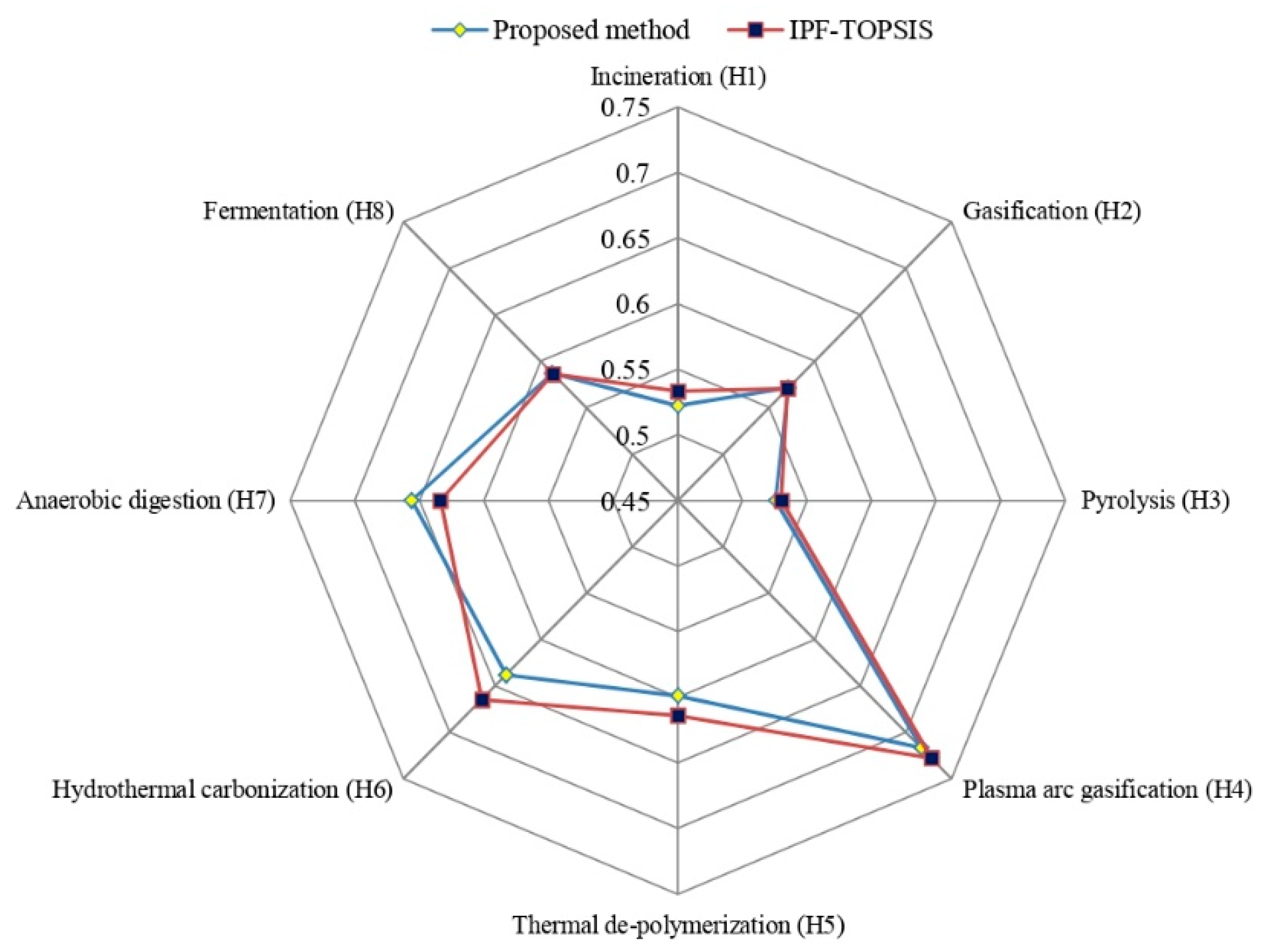
Comparison with Existing Methods

In the current part of the study, we discuss a comparison between the presented method and the extant IPF-TOPSIS model [57] for solving MCDM problems under IPFS context.

• IPF-TOPSIS Approach

Steps 1–4: Follow the steps of the IPF-COPRAS method.

Step 5: Obtain the “normalized A-IPF-DM (N-A-IPF-DM)”.

The N-A-IPF-DM $\mathbb{Q}={\left[{\varsigma }_{ij}\right]}_{s\hspace{0.17em}\times \hspace{0.17em}t}$ is assessed from $\stackrel{⌢}{Z}={\left({\stackrel{⌢}{\mathsf{\delta }}}_{ij}\right)}_{s\hspace{0.17em}\times \hspace{0.17em}t},$ is given by

$${\varsigma }_{ij}=\{\begin{array}{l}{\stackrel{⌢}{\mathsf{\delta }}}_{ij}=\hspace{0.17em}{\left(\left[{\mathsf{\mu }}_{ij}^{-},\hspace{0.17em}{\mathsf{\mu }}_{ij}^{+}\right],\hspace{0.17em}\left[{\mathsf{\nu }}_{ij}^{-},\hspace{0.17em}{\mathsf{\nu }}_{ij}^{+}\right]\right)}_{s\hspace{0.17em}\times \hspace{0.17em}t},\hspace{0.17em}\hspace{0.17em}\hspace{0.17em}\hspace{0.17em}\hspace{0.17em}\hspace{0.17em}\hspace{0.17em}\hspace{0.17em}\hspace{0.17em}\hspace{0.17em}\mathrm{for}\hspace{0.17em}\hspace{0.17em}\mathrm{benefit}\hspace{0.17em}\hspace{0.17em}\mathrm{criterion},\\ {\left({\stackrel{⌢}{\mathsf{\delta }}}_{ij}\right)}^c={\left(\left[{\mathsf{\nu }}_{ij}^{-},\hspace{0.17em}{\mathsf{\nu }}_{ij}^{+}\right],\hspace{0.17em}\hspace{0.17em}\left[{\mathsf{\mu }}_{ij}^{-},\hspace{0.17em}{\mathsf{\mu }}_{ij}^{+}\right]\right)}_{s\hspace{0.17em}\times \hspace{0.17em}t},\hspace{0.17em}\hspace{0.17em}\mathrm{for}\hspace{0.17em}\hspace{0.17em}\cos \mathrm{t}\hspace{0.17em}\hspace{0.17em}\mathrm{criterion}.\end{array}$$

(29)

Step 6: Calculate the discriminations of each alternative from “interval-valued Pythagorean fuzzy-ideal solution (IPF-IS)” and “interval-valued Pythagorean fuzzy-anti ideal solution (IPF-A-IS)”.

Here, the interval-valued BD and NBD of IPF-IS are defined as 1 and 0, and they are given as follows ${\theta }^{+}={\langle \left[1,1\right],\left[0,0\right]\rangle }_{1\times t}.$ Similarly, IPF-A-IS is as follows ${\theta }^{-}={\langle \left[0,0\right],\hspace{0.17em}\hspace{0.17em}\left[1,1\right]\rangle }_{1\times n}.$

To obtain the diverse alternative(s) $H_i:i=1\left(1\right)s,$ compute the distance measures by

$$d\left(H_i,\hspace{0.17em}{\theta }^{+}\right)=\sqrt{{\displaystyle \sum _{j=1}^n{\left\{w_j{\left(\mathbb{S}\left({\theta }^{+}\right)-\mathbb{S}\left({\varsigma }_{ij}\right)\right)}^2\right\}}^2}},$$

(30)

and

$$d\left(H_i,\hspace{0.17em}{\theta }^{-}\right)=\sqrt{{\displaystyle \sum _{j=1}^n{\left\{w_j{\left(\mathbb{S}\left({\varsigma }_{ij}\right)-\mathbb{S}\left({\theta }^{-}\right)\right)}^2\right\}}^2}},$$

(31)

Step 7: Compute the “closeness index (CI)”.

The CI of an alternative is determined by

$$ℂ\left(H_i\right)=\frac{d\left(H_i,\hspace{0.17em}{\theta }^{-}\right)}{d\left(H_i,\hspace{0.17em}{\theta }^{-}\right)+d\left(H_i,\hspace{0.17em}{\theta }^{+}\right)},\hspace{0.17em}i=1\left(1\right)s.$$

(32)

Step 8: Determine the prioritization of the options.

Corresponding to the preference ranking of $ℂ\left(H_i\right):i=1\left(1\right)s,$ we prioritize the options, and thus, we obtain the most appropriate candidate(s).

Through the use of Table 6 and Equation (29), the N-A-IPF-DM is evaluated and given in

Table 9. The N-A-IPF-DM of WTE technology for MSW treatment alternatives.

	H1	H2	H3	H4	H5	H6	H7	H8
P1	([0.814,0.864], [0.177, 0.275])	([0.745, 0.823], [0.259, 0.358])	([0.660,0.753], [0.346, 0.445])	([0.546, 0.646], [0.467, 0.597])	([0.629, 0.729], [0.375, 0.484])	([0.588, 0.685], [0.421, 0.549])	([0.782, 0.856], [0.152, 0.248])	([0.826, 0.876], [0.155, 0.252])
P2	([0.636,0.732], [0.369, 0.468])	([0.716, 0.798], [0.293, 0.386])	([0.590,0.691], [0.417, 0.547])	([0.679, 0.775], [0.325, 0.425])	([0.611, 0.705], [0.402, 0.532])	([0.709, 0.790], [0.300, 0.398])	([0.814, 0.864], [0.178, 0.276])	([0.741, 0.821], [0.263, 0.362])
P3	([0.484,0.621], [0.528, 0.629])	([0.578, 0.728], [0.459, 0.560])	([0.455,0.596], [0.564, 0.666])	([0.719, 0.835], [0.295, 0.444])	([0.571, 0.718], [0.468, 0.569])	([0.670, 0.795], [0.348, 0.489])	([0.447, 0.574], [0.555, 0.655])	([0.447, 0.581], [0.605, 0.692])
P4	([0.467,0.597], [0.546, 0.646])	([0.529, 0.675], [0.495, 0.596])	([0.571,0.718], [0.468, 0.569])	([0.788, 0.893], [0.215, 0.363])	([0.455, 0.596], [0.564, 0.666])	([0.590, 0.742], [0.444, 0.544])	([0.589, 0.741], [0.452, 0.554])	([0.519, 0.669], [0.498, 0.599])
P5	([0.480,0.616], [0.532, 0.633])	([0.650, 0.771], [0.368, 0.512])	([0.551,0.694], [0.487, 0.589])	([0.578, 0.728], [0.459, 0.560])	([0.461, 0.598], [0.560, 0.655])	([0.544, 0.690], [0.505, 0.608])	([0.733, 0.856], [0.289, 0.423])	([0.586, 0.737], [0.469, 0.571])
P6	([0.589,0.741], [0.452, 0.554])	([0.525, 0.674], [0.490, 0.590])	([0.717,0.841], [0.307, 0.445])	([0.554, 0.701], [0.479, 0.580])	([0.443, 0.569], [0.558, 0.659])	([0.425, 0.540], [0.591, 0.692])	([0.439, 0.553], [0.575, 0.676])	([0.680, 0.806], [0.349, 0.492])
P7	([0.498,0.637], [0.520, 0.621])	([0.573, 0.712], [0.440, 0.562])	([0.589,0.741], [0.452, 0.554])	([0.453, 0.582], [0.573, 0.674])	([0.518, 0.659], [0.508, 0.609])	([0.483, 0.618], [0.538, 0.640])	([0.551, 0.687], [0.472, 0.586])	([0.585, 0.725], [0.425, 0.545])
P8	([0.478,0.614], [0.546, 0.644])	([0.553, 0.684], [0.464, 0.587])	([0.592,0.744], [0.463, 0.560])	([0.687, 0.820], [0.347, 0.474])	([0.565, 0.717], [0.473, 0.572])	([0.580, 0.733], [0.451, 0.551])	([0.546, 0.697], [0.518, 0.612])	([0.463, 0.596], [0.581, 0.673])
P9	([0.501,0.641], [0.516, 0.617])	([0.258, 0.364], [0.752, 0.825])	([0.370,0.484], [0.641, 0.731])	([0.767, 0.879], [0.243, 0.387])	([0.694, 0.820], [0.327, 0.464])	([0.628, 0.754], [0.408, 0.552])	([0.754, 0.867], [0.258, 0.407])	([0.493, 0.638], [0.542, 0.645])
P10	([0.578,0.728], [0.459, 0.560])	([0.494, 0.625], [0.535, 0.637])	([0.494,0.625], [0.535, 0.637])	([0.657, 0.790], [0.378, 0.506])	([0.697, 0.824], [0.323, 0.459])	([0.702, 0.829], [0.317, 0.452])	([0.518, 0.659], [0.508, 0.609])	([0.582, 0.717], [0.437, 0.559])
P11	([0.484,0.621], [0.528, 0.629])	([0.586, 0.738], [0.459, 0.557])	([0.522,0.670], [0.526, 0.625])	([0.721, 0.840], [0.287, 0.433])	([0.541, 0.686], [0.496, 0.598])	([0.589, 0.741], [0.452, 0.554])	([0.628, 0.779], [0.424, 0.525])	([0.613, 0.740], [0.419, 0.551])
P12	([0.467,0.597], [0.546, 0.646])	([0.501, 0.641], [0.516, 0.617])	([0.571,0.718], [0.468, 0.569])	([0.688, 0.807], [0.340, 0.493])	([0.553, 0.704], [0.482, 0.584])	([0.586, 0.737], [0.469, 0.571])	([0.568, 0.720], [0.467, 0.568])	([0.663, 0.795], [0.367, 0.496])

. Now, the overall outcomes of the IPF-TOPSIS are given in

Table 10. Ranking orders of IPF-TOPSIS for MSW treatment alternatives.

Options				Ranking
H1	1.3637	1.5584	0.5333	7
H2	1.3052	1.7313	0.5702	6
H3	1.3731	1.5504	0.5303	8
H4	0.8129	2.1736	0.7278	1
H5	1.1240	1.7870	0.6139	4
H6	0.9754	1.9340	0.6647	2
H7	1.1169	1.9328	0.6338	3
H8	1.2431	1.7621	0.5864	5

.

The comparative results shown in Table 10 demonstrate that the most optimal WTE technology for MSW treatment option is $H_4$, and ranking orders obtained by the proposed IPF-COPRAS model show great conformity with the IPF-TOPSIS [57] approach. As compared with the IPF-TOPSIS (Garg, 2017) approach, the ranking order is $H_4\succ H_6\succ H_7\succ H_5\succ H_8\succ H_2\succ H_1\succ H_3,$ whereas compared with the IPF-COPRAS method, the ranking order is $H_4\succ H_7\succ H_6\succ H_5\succ H_8\succ H_2\succ H_3\succ H_1.$ From Table 8 and Table 10, it is observed that the alternative plasma arc gasification $\left(H_4\right)$ has the highest UD in all the approaches.

As per the comparative study, the developed IPF-COPRAS approach has the following merits over the existing ones, as given in Figure 5:

−

In our approach, the weights of DEs are found with the help of the proposed formula based on Liu and Wang [54], ensuring a more accurate individual significance degree of DEs. Next, the optimal criteria weights in our methodology are obtained through the proposed similarity measure and LP optimization method, which results in outcomes that are more precise and optimal weights, unlike the arbitrarily chosen criteria’s weights by decision-makers in Garg [57].

−

In [57], the alternatives are prioritized using the relative closeness coefficient between the overall value of the alternative and the ideal alternative. In the IPF-COPRAS method, the benefit and the cost criteria are both considered. Considering that both the benefit and cost criteria with complex proportions contain more precise data than both the benefit criteria or cost criteria. Meanwhile, it increases the reliability of initial data and the precision of results as well.

−

In [57], the distance is calculated between the overall attribute value of an alternative and the IVP-IS ${\mathsf{\vartheta }}^{+}={\langle \left[1,1\right],\left[0,0\right]\rangle }_{1\times n}$ and the IPF-AIS ${\mathsf{\vartheta }}^{-}={\langle \left[0,0\right],\hspace{0.17em}\hspace{0.17em}\left[1,1\right]\rangle }_{1\times n}$ to define the CI of each alternative on the given attributes. The IPF-IS and IPF-AIS may be treated as benchmarks against which the performance of the alternatives on each attribute is evaluated. Note that these benchmarks are too unrealistic to be achieved in practice. On the other hand, the COPRAS approach assumes both concerns of criteria according to the complex proportional evaluation, which holds more precise information than diverse existing methods basically considering the beneficial or non-beneficial attributes. Thus, in the process, the benchmarks are obtained on IPF-IS, IPF-AIS, similarity measure and compromise solution, which are more realistic in the sense that the decision-maker knows not only about the best and worst performance of alternatives on the given attributes but also a relative comparison of the performances among them.

−

When the number of criteria or options becomes very large, the IPF-COPRAS approach has more operability than the IPF-TOPSIS. In the IPF-COPRAS approach, there is no requirement to obtain the IPF-IS and the IPF-A-IS. The decision outcomes can be obtained through processing the realistic information, which allows the IPF-COPRAS approach to apply more intricate and realistic MCDM problems.

6. Conclusions

The present study introduces an “interval-valued Pythagorean fuzzy-complex proportional assessment (IPF-COPRAS)” method for assessing the “waste-to-energy (WTE)” technologies for “municipal solid waste (MSW)” treatment. This method is based on “similarity measure (SM)”, a linear programming model and the “complex proportional assessment (COPRAS)” approach within “interval-valued Pythagorean fuzzy sets (IPFSs)”. First, a novel formula has been introduced to estimate the “decision expert’s (DE’s)” weight. Second, in order to depict the criteria weights, a novel SM has been developed for “interval-valued Pythagorean fuzzy sets”. A comparison with extant similarity measures has been made to show the utility of the proposed similarity IPF-SM. A linear programming model has been developed using the proposed similarity measure to compute the criteria’s weights. In addition, a case study of WTE selection technologies for MSW treatment has been taken to show the feasibility of the presented IPF-COPRAS method. A comparison with extant method has been given to verify the outcomes found by the presented methodology. Thus, to handle with the “multi-criteria decision-making (MCDM)” problems, the IPF-COPRAS method provides an easy procedure of calculation with efficient and precise outcomes. Based on the analysis, the considered criteria are categorized in two dimensions, namely qualitative and quantitative dimensions. The most important criteria for selecting the appropriate WTE technology for MSW treatment are “greenhouse gas (GHG)” emissions, microbial inactivation efficacy, air emissions avoidance and public acceptance with the significance degree of 0.200 and 0.100, respectively. The evaluation results showed that the most appropriate WTE technology for MSW treatment is plasma arc gasification with a maximum utility degree of 0.717 followed by anaerobic digestion with a utility degree of 0.656 based on the identified criteria, which will assist with reducing the amount of waste and GHG emissions as well as minimizing and maintaining the costs of landfills.

The certain limitations of the developed framework are important to be aware of. A practical difficulty is that decision experts must be trained with the preference style to properly utilize the flexibility and potential of IPFSs. In the following, we present the limitations of the introduced decision-making methodology. (a) An objective weighting procedure is applied to obtain the significance weight value of criteria that is determined from the decision matrices and is derived according to the knowledge presented by experts. (b) As the waste-to-energy technology selection problem becomes increasingly serious, more dimensions of sustainability should be considered in waste-to-energy technology assessment. Furthermore, the developed methodology will be extended to “intuitionistic fuzzy hypersoft sets”, “complex spherical fuzzy N-soft sets” and “semiring-valued fuzzy sets”.

The MSW management is a concern for the environmental engineers, township developers and the local community due to its increasing amount and limited land resources. This leads to the objective whereby most of the latest efforts concentrate on “zero waste” and/or “zero landfilling”, which is indeed expensive [71] for less economy. Around 55% capacity on MSW landfills can be reduced using the “refuse derived fuel (RDF)” in the cement firms. It is a better choice for the eco-friendly disposal and for improving its energy potential, but it has area restrictions. The comprehensive procedure of MSW management is not viable for the small local community because of a lack of financial supports [72]. Hence, developing nations should find area-specific solutions to their concerns [73] in the MSW management. The application of a “plasma gasification process (PGP)” in “waste-to-energy” relieves the pressure on distressed landfills and provides an environmentally benign procedure of disposing MSW [74]. The MSW is considered as a “renewable energy source”, and the “plasma gasification technology” is one of the leading-edge procedures available to harness this energy.

In the recent past, the “United States (US)” government officially stated the MSW as a “renewable source of energy”, and power generation with the use of MSW is considered green power and capable for all suitable incentives. The elucidation is described as “Prescription for the planet: the painless remedy for our energy & environmental crises” [74]. Plasma technology purports to be an economic and ample source of energy as well as a reliable source of power. Viewing to various implementations of the plasma gasification procedure, the profit potential of plasma conversion is tremendous [74]. Private firms could construct facilities in developing nations, and it would naturally be in their financial best interest to create the garbage collection infrastructure to assist their business; indirectly, the collection process will be upgraded. This is an impeccable niche for the oil firms. Plasma converters characterize the ultimate in recycling, building virtually 100% of the waste a household usually generates into usable and even valuable end products [74]. There would be no requirement to have two garbage pickups every week, one for trash and one for recyclables that societies have become accustomed to separating. The plasma gasification procedure of MSW has all the qualities of implementation; while there are several divergences among scientists and policy-makers on these concerns, there is, however, agreement that option sources of energy that are sustainable, environmentally friendly and locally accessible must be the best alternative.

The sustainability of any MSW management scheme depends on various factors [75]; however, the most significant one is the will of the people/society to change the extant procedure and create something better. The acceptance of latest technologies has to be taken into account as well as the selection of a waste management system. However, for any MSW management to be successful, the government or firms should step up and take the vital initiatives. Although financial restraints are a part of the scheme, the government can make a proper and sincere assurance for eradicating garbage from the planet. There is a requirement to create environmental awareness and change the behavior of people/societies regarding waste for sustainable waste management organizations. Now, the government and societies of India are trying to take several actions concerning MSW management and to produce energy from waste.

References

1. Qazi, W.A.; Abushammala, M.F.M.; Azam, M.H. Multi-criteria decision analysis of waste-to-energy technologies for municipal solid waste management in Sultanate of Oman. Waste Manag. Res. 2018, 36, 594–605. [Google Scholar] [CrossRef] [PubMed]
2. Hereher, M.E.; Al-Awadhi, T.; Mansour, S.A. Assessment of the optimized sanitary landfill sites in Muscat, Oman. Egypt. J. Remote Sens. Space Sci. 2019, 23, 355–362. [Google Scholar] [CrossRef]
3. Joshi, R.; Ahmed, S. Status and challenges of municipal solid waste management in India: A review. Cogent Environ. Sci. 2016, 2, 1139434. [Google Scholar] [CrossRef]
4. Dutta, A.; Jinsart, W. Waste generation and management status in the fast-expanding Indian cities: A review. J. Air Waste Manag. Assoc. 2020, 70, 491–503. [Google Scholar] [CrossRef]
5. Kaza, S.; Yao, L.; Bhad-Tata, P.; Woerden, F.V. What a Waste 2.0: A Global Snapshot of Solid Waste 2050; The World Bank: Washington, DC, USA, 2018. [Google Scholar] [CrossRef]
6. Mayer, F.; Bhandari, R.; Gäth, S. Critical review on life cycle assessment of conventional and innovative waste-to-energy technologies. Sci. Tot. Environ. 2019, 672, 708–721. [Google Scholar] [CrossRef] [PubMed]
7. Moya, D.; Aldás, C.; López, G.; Kaparaju, P. Municipal solid waste as a valuable renewable energy resource: A worldwide opportunity of energy recovery by using waste-to-energy technologies. Energy Proc. 2017, 134, 286–295. [Google Scholar] [CrossRef]
8. Tsui, T.; Wong, J.W.C. A critical review: Emerging bioeconomy and waste-to-energy technologies for sustainable municipal solid waste management. Waste Dispos. Sustain. Energy 2019, 1, 151–167. [Google Scholar] [CrossRef] [Green Version]
9. Yadav, P.; Samadder, S.R. A global prospective of income distribution and its effect on life cycle assessment of municipal solid waste management: A review. Environ. Sci. Pollut. Res. 2017, 24, 9123–9141. [Google Scholar] [CrossRef] [Green Version]
10. D’Adamo, I.; Gastaldi, M.; Rosa, P. Recycling of end-of-life vehicles: Assessing trends and performances in Europe. Technol. Forecast. Soc. Chang. 2020, 152, 119887. [Google Scholar] [CrossRef]
11. Noya, I.; Inglezakis, V.; González-García, S.; Katsou, E.; Feijoo, G.; Moreira, M.T. Comparative environmental assessment of alternative waste management strategies in developing regions: A case study in Kazakhstan. Waste Manag. Res. 2018, 36, 689–697. [Google Scholar] [CrossRef]
12. Farooq, A.; Haputta, P.; Silalertruksa, T.; Gheewala, S.H. Framework for the Selection of Suitable Waste to Energy Technologies for a Sustainable Municipal Solid Waste Management System. Front. Sustain. 2021, 2, 27. [Google Scholar] [CrossRef]
13. Farooq, A.; Bangviwat, A.; Gheewala, S. Life cycle cost analysis of ethanol production from sugarcane molasses for gasoline substitution as transportation fuel in Pakistan. J. Sustain. Energy Environ. 2020, 11, 49–59. [Google Scholar]
14. Giri, B.C.; Dey, S. Game theoretic models for a closed-loop supply chain with stochastic demand and backup supplier under dual channel recycling. Decis. Mak. Appl. Manag. Eng. 2020, 3, 108–125. [Google Scholar] [CrossRef]
15. Badi, I.; Abdulshahed, A.; Shetwan, A.; Eltayeb, W. Evaluation of solid waste treatment methods in Libya by using the analytic hierarchy process. Decis. Mak. Appl. Manag. Eng. 2019, 2, 19–35. [Google Scholar] [CrossRef]
16. Ayodele, T.R.; Ogunjuyigbe, A.S.O.; Alao, M.A. Life cycle assessment of waste-to-energy (WtE) technologies for electricity generation using municipal solid waste in Nigeria. Appl. Energy 2017, 201, 200–218. [Google Scholar] [CrossRef]
17. Khan, I.; Kabir, Z. Waste-to-energy generation technologies and the developing economies: A multi-criteria analysis for sustainability assessment. Renew. Energy 2020, 150, 320–333. [Google Scholar] [CrossRef]
18. Beyene, H.D.; Werkneh, A.A.; Ambaye, T.G. Current updates on waste to energy (WtE) technologies: A review. Renew. Energy Focus. 2018, 24, 1–11. [Google Scholar] [CrossRef]
19. Kurbatova, A.; Abu-Qdais, H.A. Using multi-criteria decision analysis to select waste to energy technology for a mega city: The case of Moscow. Sustainability 2020, 12, 9828. [Google Scholar] [CrossRef]
20. Kumar, A.; Agrawal, A. Recent trends in solid waste management status, challenges, and potential for the future Indian cities—A review. Curr. Res. Environ. Sustain. 2020, 2, 100011. [Google Scholar] [CrossRef]
21. Ali, Z.; Mahmood, T.; Ullah, K.; Khan, Q. Einstein Geometric Aggregation Operators using a Novel Complex Interval-valued Pythagorean Fuzzy Setting with Application in Green Supplier Chain Management. Rep. Mech. Eng. 2021, 2, 105–134. [Google Scholar] [CrossRef]
22. Zadeh, L.A. Fuzzy sets. Inf. Control. 1965, 8, 338–353. [Google Scholar] [CrossRef] [Green Version]
23. Atanassov, K.T. Intuitionistic fuzzy sets. Fuzzy Sets Syst. 1986, 20, 87–96. [Google Scholar] [CrossRef]
24. Atanassov, K.; Gargov, G. Interval valued intuitionistic fuzzy sets. Fuzzy Sets Syst. 1989, 31, 343–349. [Google Scholar] [CrossRef]
25. Yager, R.R. Pythagorean membership grades in multicriteria decision making. IEEE Trans. Fuzzy Syst. 2014, 22, 958–965. [Google Scholar] [CrossRef]
26. Ashraf, A.; Ullah, K.; Hussain, A.; Bari, M. Interval-Valued Picture Fuzzy Maclaurin Symmetric Mean Operator with application in Multiple Attribute Decision-Making. Rep. Mech. Eng. 2022, 3, 301–317. [Google Scholar] [CrossRef]
27. Mahmood, T.; Ali, Z. Analysis of Maclaurin Symmetric Mean Operators for Managing Complex Interval-valued q-Rung Orthopair Fuzzy Setting and Their Applications: MSM Operators for Managing CIVq-ROFS. J. Comput. Cogn. Eng. 2022, 1–18. [Google Scholar] [CrossRef]
28. Bakioglu, G.; Atahan, A.O. AHP integrated TOPSIS and VIKOR methods with Pythagorean fuzzy sets to prioritize risks in self-driving vehicles. Appl. Soft Comput. 2021, 99, 106948. [Google Scholar] [CrossRef]
29. Liu, P.; Rani, P.; Mishra, A.R. A novel Pythagorean fuzzy combined compromise solution framework for the assessment of medical waste treatment technology. J. Clean. Prod. 2021, 292, 126047. [Google Scholar] [CrossRef]
30. Khan, R.; Ullah, K.; Pamucar, D.; Bari, M. Performance Measure Using a Multi-Attribute Decision Making Approach Based on Complex T-Spherical Fuzzy Power Aggregation Operators. J. Comput. Cogn. Eng. 2022, 1–9. [Google Scholar] [CrossRef]
31. Firozja, M.A.; Agheli, B.; Jamkhaneh, E.B. A new similarity measure for Pythagorean fuzzy sets. Complex Intell. Syst. 2020, 6, 67–74. [Google Scholar] [CrossRef] [Green Version]
32. Rani, P.; Mishra, A.R.; Pardasani, K.R.; Mardani, A.; Liao, H.; Streimikiene, D. A novel VIKOR approach based on entropy and divergence measures of Pythagorean fuzzy sets to evaluate renewable energy technologies in India. J. Clean. Prod. 2019, 239, 117936. [Google Scholar] [CrossRef]
33. Peng, X.; Yang, Y. Fundamental properties of interval-valued Pythagorean fuzzy aggregation operators. Int. J. Intell. Syst. 2016, 31, 444–487. [Google Scholar] [CrossRef]
34. He, J.; Huang, Z.; Mishra, A.R.; Alrasheedi, M. Developing a new framework for conceptualizing the emerging sustainable community-based tourism using an extended interval-valued Pythagorean fuzzy SWARA-MULTIMOORA. Technol. Forecast. Soc. Change 2021, 171, 120955. [Google Scholar] [CrossRef]
35. Chen, T.Y. A novel VIKOR method with an application to multiple criteria decision analysis for hospital-based post-acute care within a highly complex uncertain environment. Neural Comput. Appl. 2019, 31, 3969–3999. [Google Scholar] [CrossRef]
36. Liang, W.; Zhang, X.; Liu, M. The maximizing deviation method based on interval-valued Pythagorean fuzzy weighted aggregating operator for multiple criteria group decision analysis. Discrete Dyn. Nat. Soc. 2015, 2015, 746572. [Google Scholar] [CrossRef]
37. Liang, D.; Darko, A.P.; Xu, Z.; Quan, W. The linear assignment method for multicriteria group decision making based on interval-valued Pythagorean fuzzy Bonferroni mean. Int. J. Intell. Syst. 2018, 33, 2101–2138. [Google Scholar] [CrossRef]
38. Rahman, K.; Abdullah, S.; Khan, M. Some interval-valued Pythagorean fuzzy Einstein weighted averaging aggregation operators and their application to group decision making. J. Intell. Syst. 2020, 29, 393–408. [Google Scholar] [CrossRef]
39. Garg, H. A linear programming method based on an improved score function for interval-valued Pythagorean fuzzy numbers and its application to decision-making. Int. J. Uncertain. Fuzziness Knowl.-Based Syst. 2018, 26, 67–80. [Google Scholar] [CrossRef]
40. Chen, T.Y. An interval-valued Pythagorean fuzzy outranking method with a closeness-based assignment model for multiple criteria decision making. Int. J. Intell. Syst. 2018, 33, 126–168. [Google Scholar] [CrossRef]
41. Peng, X.; Li, W. Algorithms for interval-valued Pythagorean fuzzy sets in emergency decision making based on multiparametric similarity measures and WDBA. IEEE Access 2019, 7, 7419–7441. [Google Scholar] [CrossRef]
42. Al-Barakati, A.; Mishra, A.R.; Mardani, A.; Rani, P. An extended interval-valued Pythagorean fuzzy WASPAS method based on new similarity measures to evaluate the renewable energy sources. Appl. Soft Comput. 2022, 120, 108689. [Google Scholar] [CrossRef]
43. Zavadskas, E.K.; Kaklauskas, A.; Sarka, V. The new method of multicriteria complex proportional assessment of projects. Technol. Econ. Dev. Econ. 1994, 1, 131–139. [Google Scholar]
44. Kumari, R.; Mishra, A.R. Multi-criteria COPRAS method based on parametric measures for intuitionistic fuzzy sets: Application of green supplier selection. Iran. J. Sci. Technol. Trans. Electr. Eng. 2020, 44, 1645–1662. [Google Scholar] [CrossRef]
45. Lu, J.; Zhang, S.; Wu, J.; Wei, Y. COPRAS method for multiple attribute group decision making under picture fuzzy environment and their application to green supplier selection. Technol. Econ. Dev. Econ. 2021, 27, 369–385. [Google Scholar] [CrossRef]
46. Mishra, A.R.; Rani, P.; Mardani, A.; Pardasani, K.R.; Govindan, K.; Alrasheedi, M. Healthcare evaluation in hazardous waste recycling using novel interval-valued intuitionistic fuzzy information based on complex proportional assessment method. Comput. Ind. Eng. 2020, 139, 106140. [Google Scholar] [CrossRef]
47. Mishra, A.R.; Rani, P.; Pardasani, K.R. Multiple-criteria decision-making for service quality selection based on Shapley COPRAS method under hesitant fuzzy sets. Granul. Comput. 2019, 4, 435–449. [Google Scholar] [CrossRef]
48. Krishankumar, R.; Garg, H.; Arun, K.; Saha, A.; Ravichandran, K.S.; Kar, S. An integrated decision-making COPRAS approach to probabilistic hesitant fuzzy set information. Complex Intell. Syst. 2021, 7, 2281–2298. [Google Scholar] [CrossRef]
49. Rani, P.; Mishra, A.R.; Mardani, A. An extended Pythagorean fuzzy complex proportional assessment approach with new entropy and score function: Application in pharmacological therapy selection for type-2 diabetes. Appl. Soft Comput. 2020, 94, 106441. [Google Scholar] [CrossRef]
50. Hezam, I.M.; Mishra, A.R.; Krishankumar, R.; Ravichandran, K.S.; Kar, S.; Pamucar, D.S. A single-valued neutrosophic decision framework for the assessment of sustainable transport investment projects based on discrimination measure. Manag. Decis. 2022. [Google Scholar] [CrossRef]
51. Roozbahini, A.; Ghased, H.; Shahedany, M.H. Inter-basin water transfer planning with grey COPRAS and fuzzy COPRAS techniques: A case study in Iranian Central Plateau. Sci. Total Environ. 2020, 726, 138499. [Google Scholar] [CrossRef]
52. Mishra, A.R.; Liu, P.; Rani, P. COPRAS method based on interval-valued hesitant Fermatean fuzzy sets and its application in selecting desalination technology. Appl. Soft Comput. 2022, 119, 108570. [Google Scholar] [CrossRef]
53. Rani, P.; Mishra, A.R.; Deveci, M.; Antucheviciene, J. New complex proportional assessment approach using Einstein aggregation operators and improved score function for interval-valued Fermatean fuzzy sets. Comput. Ind. Eng. 2022, 169, 108165. [Google Scholar] [CrossRef]
54. Liu, H.W.; Wang, G.J. Multi-criteria decision-making methods based on intuitionistic fuzzy sets. Eur. J. Oper. Res. 2007, 179, 220–233. [Google Scholar] [CrossRef]
55. Zhang, X.; Xu, Z. Extension of TOPSIS to multiple criteria decision making with Pythagorean fuzzy sets. Int. J. Intell. Syst. 2014, 29, 1061–1078. [Google Scholar] [CrossRef]
56. Zhang, X.L. A Novel Approach Based on Similarity Measure for Pythagorean Fuzzy Multiple Criteria Group Decision Making. Int. J. Intell. Syst. 2016, 31, 593–611. [Google Scholar] [CrossRef]
57. Garg, H. A novel improved accuracy function for interval valued Pythagorean fuzzy sets and its applications in the decision-making process. Int. J. Intell. Syst. 2017, 32, 1247–1260. [Google Scholar] [CrossRef]
58. Peng, X.D.; Yuan, H.Y.; Yang, Y. Pythagorean Fuzzy Information Measures and their Applications. Int. J. Intell. Syst. 2017, 32, 991–1029. [Google Scholar] [CrossRef]
59. Zhang, Q.; Hu, J.; Feng, J.; Liu, A. Multiple criteria decision making method based on the new similarity measures of Pythagorean fuzzy set. J. Intell. Fuzzy Syst. 2020, 39, 809–820. [Google Scholar] [CrossRef]
60. Mishra, A.R.; Rani, P.; Prajapati, R.S. Multi-criteria weighted aggregated sum product assessment method for sustainable biomass crop selection problem using single-valued neutrosophic sets. Appl. Soft Comput. 2021, 113, 108038. [Google Scholar] [CrossRef]
61. Ejegwa, P.A.; Agbetayo, J.M. Similarity-Distance Decision-Making Technique and its Applications via Intuitionistic Fuzzy Pairs. J. Comput. Cogn. Eng. 2022, 1–7. [Google Scholar] [CrossRef]
62. Mishra, A.R.; Rani, P.; Saha, A.; Hezam, I.M.; Pamucar, D.; Marinovic, M.; Pandey, K. Assessing the Adaptation of Internet of Things (IoT) Barriers for Smart Cities’ Waste Management Using Fermatean Fuzzy Combined Compromise Solution Approach. IEEE Access 2022, 10, 37109–37130. [Google Scholar] [CrossRef]
63. Biswas, A.; Sarkar, B. Interval-valued Pythagorean fuzzy TODIM approach through point operator-based similarity measures for multicriteria group decision making. Kybernetes 2019, 48, 496–519. [Google Scholar] [CrossRef]
64. Rani, P.; Mishra, A.R. Novel Single-Valued Neutrosophic Combined Compromise Solution Approach for Sustainable Waste Electrical and Electronics Equipment Recycling Partner Selection. IEEE Trans. Eng. Manag. 2020, 1–15. [Google Scholar] [CrossRef]
65. Mishra, A.R.; Rani, P.; Saha, A. Single-valued neutrosophic similarity measure-based additive ratio assessment framework for optimal site selection of electric vehicle charging station. Int. J. Intell. Syst. 2021, 36, 5573–5604. [Google Scholar] [CrossRef]
66. Ünver, M.; Olgun, M.; Türkarslan, E. Cosine and cotangent similarity measures based on choquet integral for spherical fuzzy sets and applications to pattern recognition. J. Comput. Cogn. Eng. 2022, 1, 21–31. [Google Scholar] [CrossRef]
67. Wang, Y.W. Interval-valued Pythagorean fuzzy TOPSIS method and its application in student recommendation. Math. Prac. Theor. 2018, 48, 108–117. [Google Scholar]
68. Soltani, A.; Sadiq, R.; Hewage, K. Selecting sustainable waste-to-energy technologies for municipal solid waste treatment: A game theory approach for group decision-making. J. Clean. Prod. 2016, 113, 388–399. [Google Scholar] [CrossRef]
69. Kumar, A.; Samadder, S.R. A review on technological options of waste to energy for effective management of municipal solid waste. Waste Manag. 2017, 69, 407–422. [Google Scholar] [CrossRef]
70. Yanmaz, O.; Turgut, Y.; Can, E.N.; Kahraman, C. Interval-valued Pythagorean fuzzy EDAS method: An application to car selection problem. J. Intell. Fuzzy Syst. 2020, 38, 4061–4077. [Google Scholar] [CrossRef]
71. Shekder, A.V. Sustainable solid waste management: An integrated approach for Asian countries. Waste Manag. 2009, 29, 1438–1448. [Google Scholar] [CrossRef]
72. Kumar, S.; Bhattacharyya, J.K.; Vaidya, A.N.; Chakrabarti, T.; Devotta, S.; Akolkar, A.B. Assessment of the status of municipal solid waste management in metro cities, state capitals, class I cities, and class II towns in India: An insight. Waste Manag. 2009, 29, 883–895. [Google Scholar] [CrossRef] [PubMed]
73. Henry, R.K.; Yongsheng, Z.; Jun, D. Country report, Municipal solid waste management challenges in developing countries—Kenyan case study. Waste Manag. 2006, 26, 92–100. [Google Scholar] [CrossRef] [PubMed]
74. Blees, T. Prescription for the Planet: The Painless Remedy for Our Energy and Environmental Crises; Charleston, S.C., Ed.; The Library of Congress: Washington, DC, USA, 2008; ISBN 1-4196-5582-5. ISBN-13 9781419655821; control number: 2008905155. [Google Scholar]
75. Gupta, M.; Srivastava, M.; Agrahari, S.K.; Detwal, P. Waste to energy technologies in India: A review. J. Energy Environ. Sustain. 2018, 6, 29–35. [Google Scholar] [CrossRef]
Figure 1. Geometrical representations of IF/IIFNs and PF/IPFNs with spaces of (a) IFNs and PFNs, (b) IIFNs and IPFNs.
Processes 10 01015 g001
Figure 2. Performance structure of the proposed IPF-COPRAS approach.
Processes 10 01015 g002
Figure 3. Hierarchical structure of WTE technology for MSW treatment assessment.
Processes 10 01015 g003
Figure 4. Criteria weight of WTE technology for MSW treatment assessment.
Processes 10 01015 g004
Figure 5. Comparison of utility degree/closeness index of each for MSW treatment.
Processes 10 01015 g005