Integration of an Absorption Chiller to a Process Applying the Pinch Analysis Approach

Nemet, Andreja; Kravanja, Zdravko; Bogataj, Miloš

doi:10.3390/pr10051028

Open AccessFeature PaperArticle

Integration of an Absorption Chiller to a Process Applying the Pinch Analysis Approach

by

Andreja Nemet

,

Zdravko Kravanja

and

Miloš Bogataj

^*

Faculty of Chemistry and Chemical Engineering, University of Maribor, SI-2000 Maribor, Slovenia

^*

Author to whom correspondence should be addressed.

Processes 2022, 10(5), 1028; https://0-doi-org.brum.beds.ac.uk/10.3390/pr10051028

Submission received: 5 April 2022 / Revised: 16 May 2022 / Accepted: 18 May 2022 / Published: 21 May 2022

(This article belongs to the Special Issue Tools, Approaches and Modeling for Energy System Design Increasing Economic and Environmental Sustainability)

Download

Browse Figures

Versions Notes

Abstract

:

In addition to the consumption of hot utilities, there is also a significant cost associated with the consumption of cold utilities when there is a high demand for cooling. A promising solution for cooling is an absorption chiller (AC), which uses heat instead of electricity for cooling. A thermodynamic approach for evaluating AC integrated with a process is presented in this work. A model for assessing the properties and duties of an AC cycle was developed. The integration of a combined process-AC system was evaluated using the Grand Composite Curve. Three different options of integration were analyzed: (i) above the Pinch, (ii) below the Pinch, and (iii) across the Pinch. AC represents the combined effect of a heat engine and a heat pump, as the generator together with the absorber and condenser has the function of a heat engine, while the evaporator combined with the absorber and condenser mimics the function of a heat pump. The comparison between the non-integrated and integrated process-AC systems has revealed that the proper placement of AC is across or below the Pinch and the improper is above the Pinch. If AC was entirely integrated below the Pinch, the integration would result in a complete (100%) reduction in the consumption of hot utility for the operation of AC. The most suitable placement of AC with double reduction of hot utility consumption and complete reduction of both hot and cold utility to operate AC is across the Pinch due to the pumping of heat through AC from below to above the Pinch.

Keywords:

absorption chiller; Pinch Analysis; heat integration; low-temperature heat

1. Introduction

Heat Integration is based on the idea of matching the heat demand with the heat surplus within comparable temperature intervals. In addition to heating, much attention is also paid to cooling demands, as these impose a significant cost on companies. An example of this is the food industry, where enormous amounts of refrigeration or freezing are required for food storage. In the UK, for example, the consumption of refrigeration in 2005 was 13.3 × 10⁹ kWh for the food and beverages industry, and 12.2 × 10⁹ kWh for the production of chemicals [1]. Instead of electricity-driven technologies, heat-driven technologies are receiving more and more attention. Nowadays, there are various types of heat-driven technologies, such as organic cycles, Kalina cycles, absorption refrigeration, and adsorption refrigeration. Different opportunities, namely the organic Rankine cycle, absorption chillers (AC), and absorption heat pumps, have been investigated for waste heat utilization from Total Site integration [2]. The presented methodology enables an evaluation of the cooling opportunities provided by the waste heat available after Total Site integration. Pátek and Klomfar [3] presented simple functions for the rapid evaluation of ammonia-water system properties that can be used for the estimation of absorption chilling properties. Sun [4] presented an approach for estimating thermodynamic data and creating a map of optimal designs to facilitate the simulation of the absorption refrigeration system. In [5], a comparison of the performance was evaluated of the NH₃-H₂O, NH₃-LiNO_3, and NH₃-NaSCN absorption refrigeration system. The author concluded that the ammonia-lithium nitrate and ammonia-sodium thiocyanate cycles are suitable alternatives to an ammonia-water absorption system. An overview of different types of generator-absorber heat exchanges can be found in [6]. The objective of this system is to improve the heat recovery within the absorption refrigeration system. Various authors studied the internal heat recovery of the absorption refrigeration cycle using Pinch Analysis (PA). Jawahar et al. [7] evaluated the thermodynamic properties of the NH₃-H₂O absorption refrigeration system, estimated the duties of the various units through simulation, and made a PA to establish a maximum internal heat recovery. A very similar approach was used by Du et al. [8], who used Grand Composite Curves (GCCs) and a modification of GCCs to evaluate heat recovery potential. There are many interesting applications of AC. An example would be utilizing waste heat generated by CPUs on a server blade from a data center to cool the other parts of the center [9]. There are also several studies that use solar energy as a heat source for a generator to cool a house [10], even in extremely hot weather [11]. An example of an installed absorption chilling driven by solar thermal energy and its operational experience can be found in [12]. Ghaebi et al. [13] proposed the integration of an AC with combined heat and power (CHP), resulting in a trigeneration system that combines heating, cooling, and power.

In addition to the numerous possible uses of absorption chilling, the two main problems with the introduction of absorption chilling should also be mentioned: (i) the large size of the cooling unit and (ii) the low coefficient of performance (COP) [14].

This paper can be seen as part of a series of papers dealing with the integration of various process equipment using the Pinch design principle. The principle is to place equipment that requires heating below the Pinch Point, and equipment releasing heat above the Pinch Point. Various rules of equipment placement have already been developed—for distillation columns [15], evaporators, heat pumps, and heat engines [16], exothermic and endothermic reactors [17], and, more recently, for compressors [18], compressors and expanders [19], and for pipe insulation [20]. In this work, the integration of absorption refrigeration with a process was evaluated using PA. The objective of the proposed methodology was to set targets and rules for the integration of an AC into the process and to provide favorable operating conditions of absorption chilling that maximize the mentioned integration. For this purpose, a model was developed for estimating the heat duties of units constituting the AC. The proper placement of AC, when integrated into the process, is evaluated, based on streams obtained from the developed model. The process alignment methodology to evaluate the potential of AC integration has been improved.

The paper is organized as follows: Section 2 presents the principle of absorption chilling and the derivation of streams for heat integration. This is followed by a description of the possible integration of AC into processes (Section 3) and the derivation of the rules for the appropriate placement of AC with respect to the Pinch. The presented theory is supported by case studies in Section 4. The main findings are listed in the Conclusions (Section 5). The thermodynamic model for AC cycle estimation is described in Appendix A.

2. Methods

2.1. Absorption Chilling

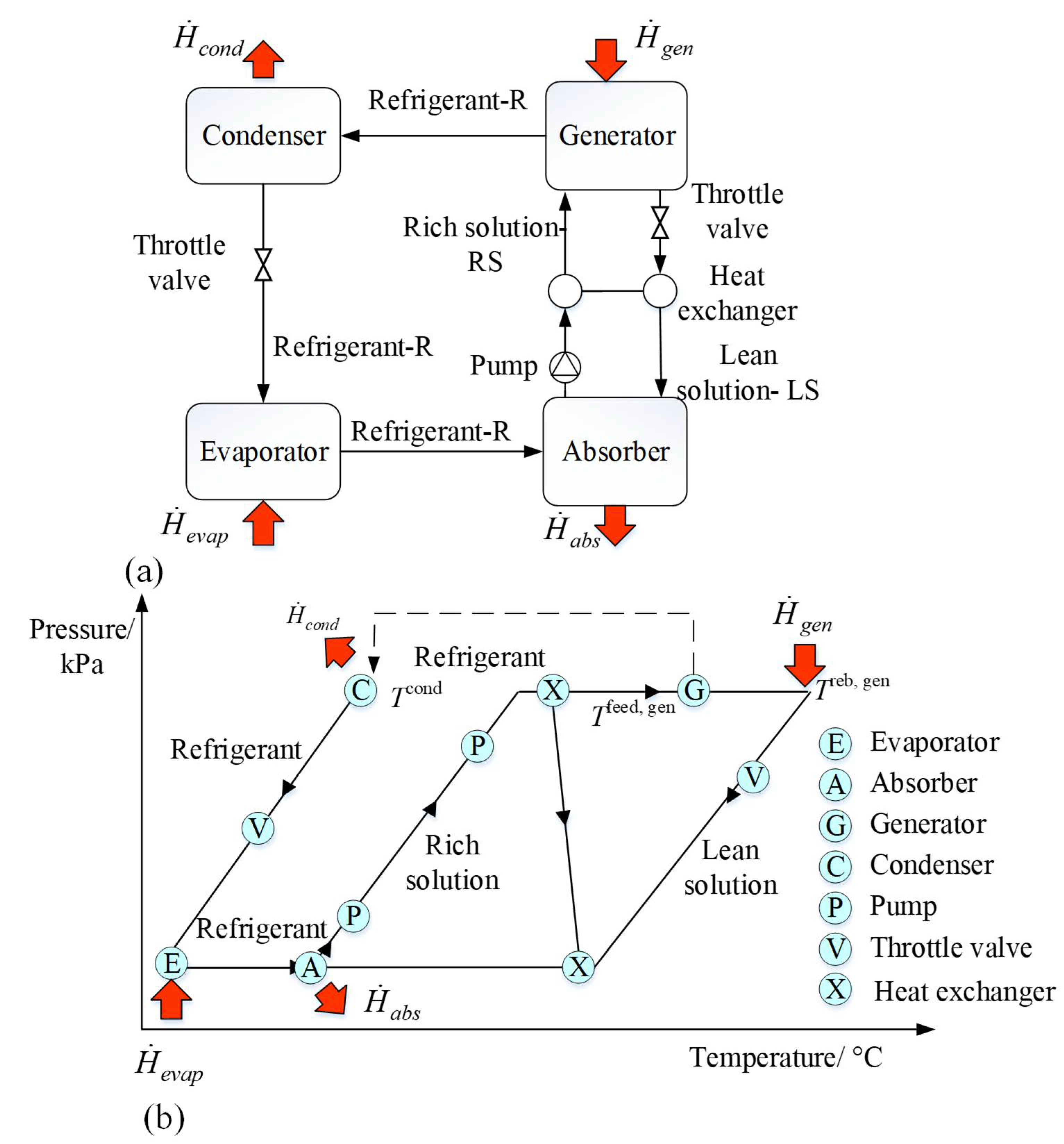
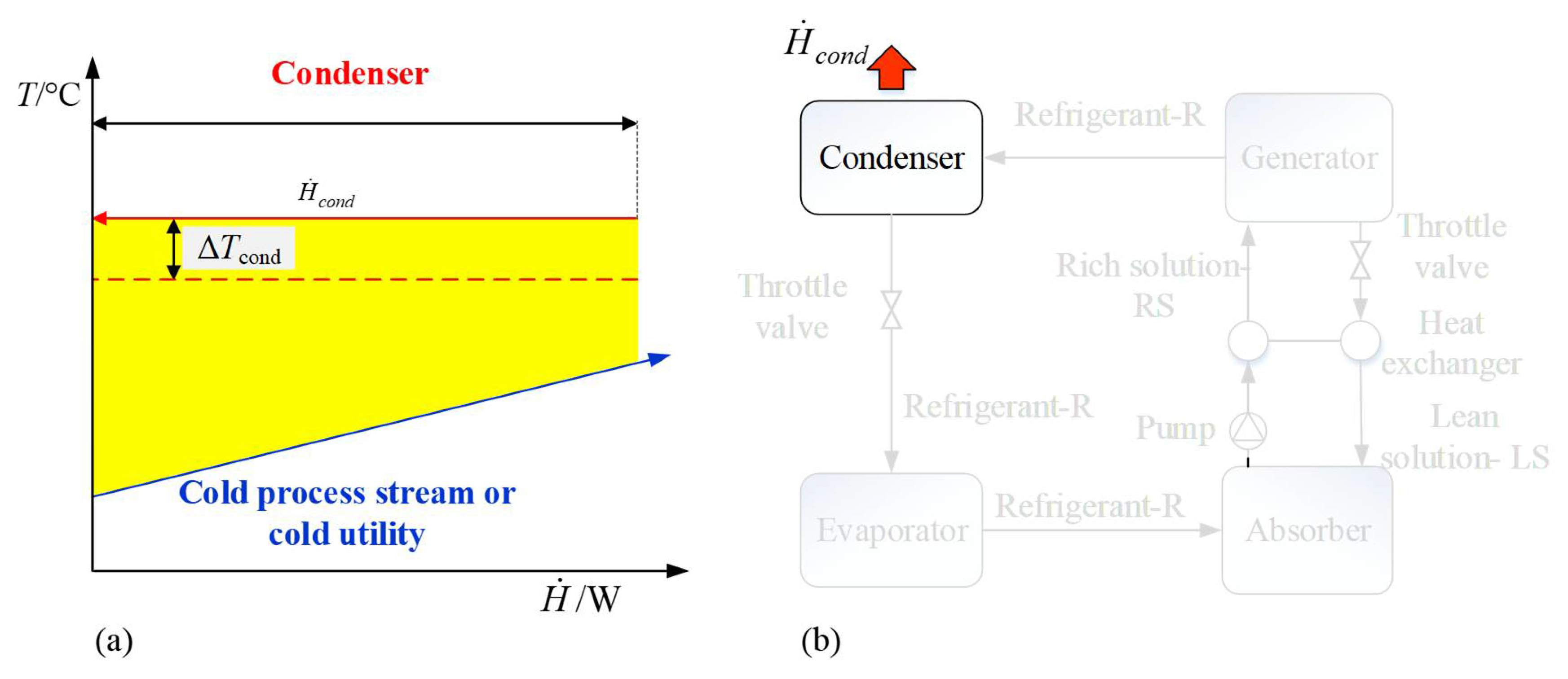
The aim of the work is to perform heat integration of AC with a process; therefore, an overview is given of the AC technology. The basic scheme for AC is presented in Figure 1a. AC consists of six main components: evaporator, absorber, pump, generator, throttle valve, and condenser. In addition, it is desirable to include a heat exchanger, to enable heat recovery within AC. The evaporator (freezer) draws heat from the area requiring cooling by evaporation at low temperature and pressure (evaporator (E) in Figure 1b). In the absorber, refrigerant from the evaporator is injected in the gas phase into a lean solution of refrigerant, producing a rich solution (absorber (A) in Figure 1b). The process is exothermic; therefore, heat should be transferred to an external cooler to maintain the required solubility. The process is presented with decreasing temperature, as the saturation temperature of the lean solution (inlet) is higher compared to the saturation temperature of the rich solution (Figure 1b). The pressure, and also the temperature of the rich solution, are increased by pumping (pump (P) in Figure 1b). The rich solution is fed into a generator at a certain feed temperature T^feed,gen (Figure 1b), where the refrigerant is evaporated from the solution under high pressure using an external heat source (generator (G) in Figure 1b). The temperature of the heat supplied from the external source should be above the temperature of the reboiler of the rectification/distillation column (generator) T^reb,gen. The remaining lean solution is fed back to the absorber. Thus, the absorber-generator forms a closed loop of lean and rich solutions. This closed-loop provides the opportunity for heat integration (heat exchanger (X) in Figure 1b) by transferring heat from the lean solution, leaving the generator with the rich solution that is sent to the generator (Figure 1a). The evaporated refrigerant is fed to the condenser to obtain a liquid phase (condenser (C) in Figure 1b). The temperature and pressure of the refrigerant are reduced by a throttle valve (throttle valve (V) in Figure 1b). The liquid refrigerant is sent to the evaporator closing the refrigerant circuit. The use of the absorber-generator offers the possibility of heat-driven cooling instead of a power-driven one.

2.2. Deriving the Representative Streams for Each Unit of Absorption Chilling

The main idea of this work is to integrate the AC with a process with maximum heat integration of the processes and the AC. A graphical representation of an AC was developed to enable the evaluation of the integration. The curves for representation of the AC components as streams are constructed as follows.

2.2.1. Evaporator

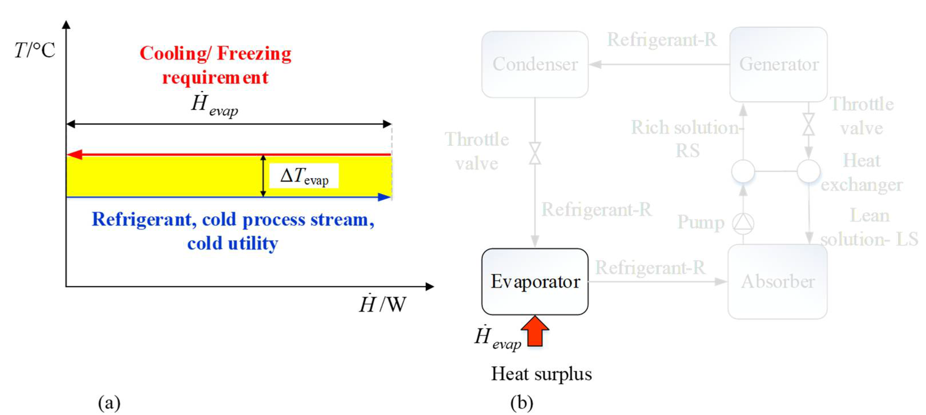
The refrigerator demand represents excess heat, which is a hot stream by definition in PA. The refrigerant should have a temperature below the required temperature of cooling to provide constant refrigeration. Therefore, to achieve feasible heat transfer, the temperature should be lowered by ΔT_min. The process of evaporation can be assumed isothermal because a phase change of one component with minimal impurities takes place. Therefore, the slope of the line is zero (Figure 2).

2.2.2. Absorber

Absorption is an exothermic process, so by definition excess heat in this component is represented as a hot stream in PA. A temperature gradient within the absorber was assumed, the temperature decreases from the equilibrium temperature of the lean solution composition to the equilibrium temperature of the rich solution composition at a given pressure. Since the cooler is usually built inside the spray tower, the temperature gradient is also reflected in the PA presentation. The excess heat from the absorption process is reduced by the preheating requirement of the refrigerant from the evaporator, so this dashed line is also included in the plot in Figure 3.

2.2.3. Rich and Lean Solutions

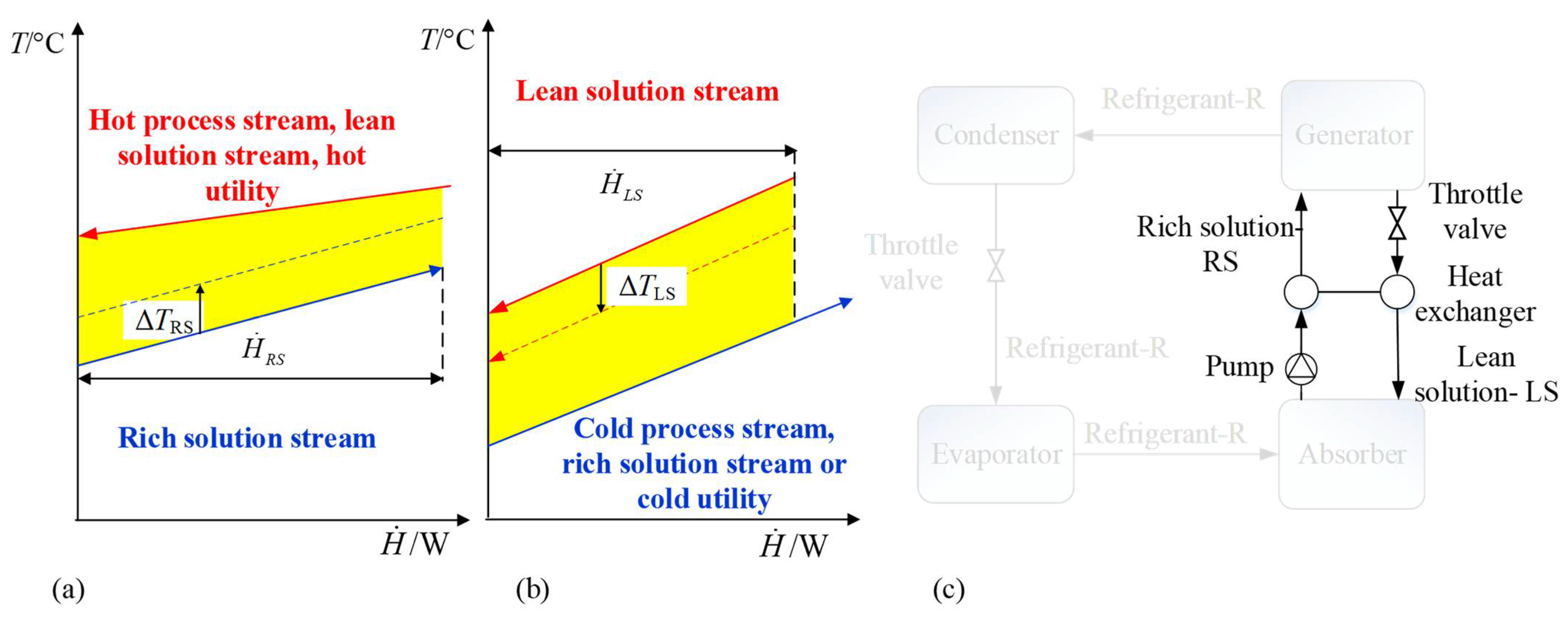
The rich solution is passed from the outlet of the lower temperature absorber to the feed tray of the higher temperature distillation column. It must be heated to reach a higher temperature; therefore, it is shown as a cold stream (Figure 4). The lean solution should be cooled down from the temperature at the bottom of the distillation column to the temperature at the inlet of the absorber, so it is represented as a hot stream. It can be seen that the rich solution stream can be heated, at least partially, with the excess heat from the lean solution stream.

2.2.4. Generator

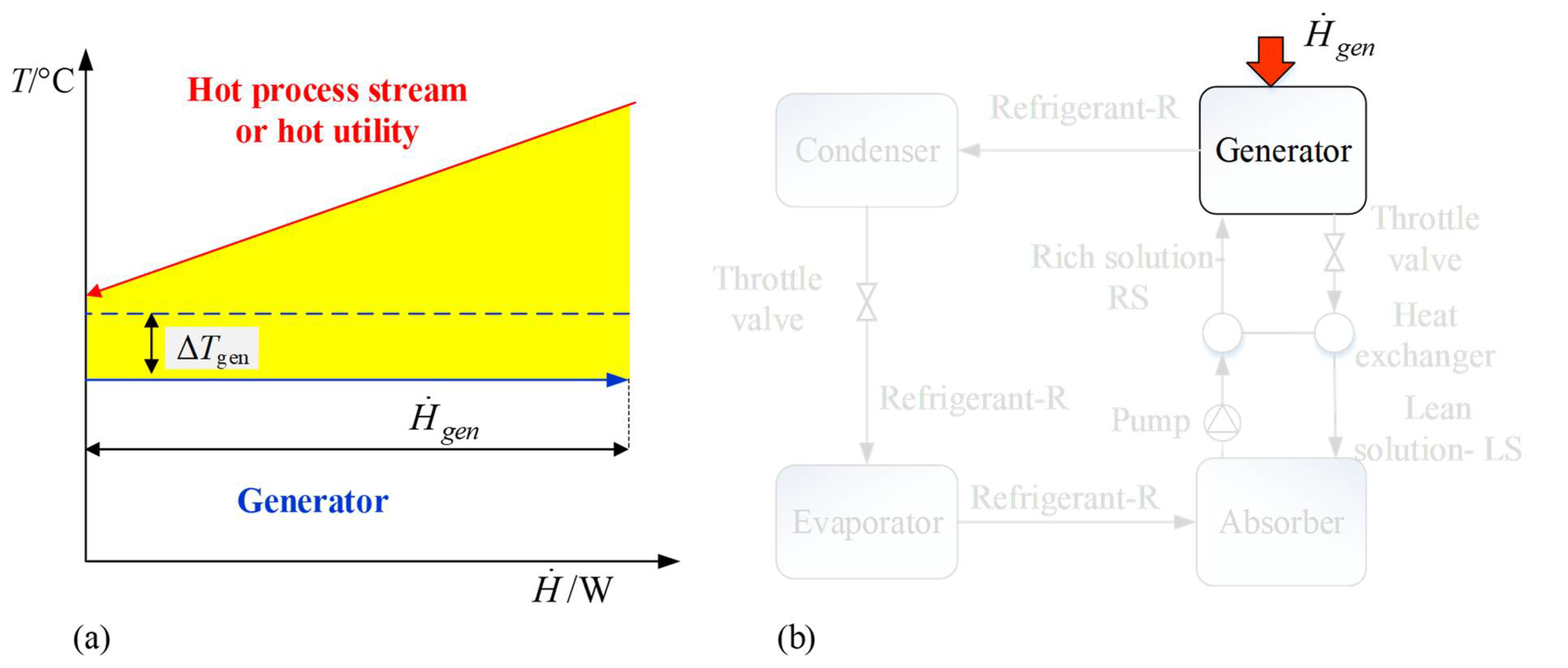
The evaporation of the refrigerant takes place in the generator. The generator line is shown as a straight line. Although the generator has a temperature gradient, the heat required is supplied only at the temperature of the reboiler, not for each tray of the distillation/rectification column separately (Figure 5).

2.2.5. Condenser

In the condenser, a phase change from vapor to liquid takes place in an exothermic process, which means excess heat. Therefore, the corresponding stream is represented as a hot stream (Figure 6). The condensation is assumed to be isothermal, and therefore, the line has no slope.

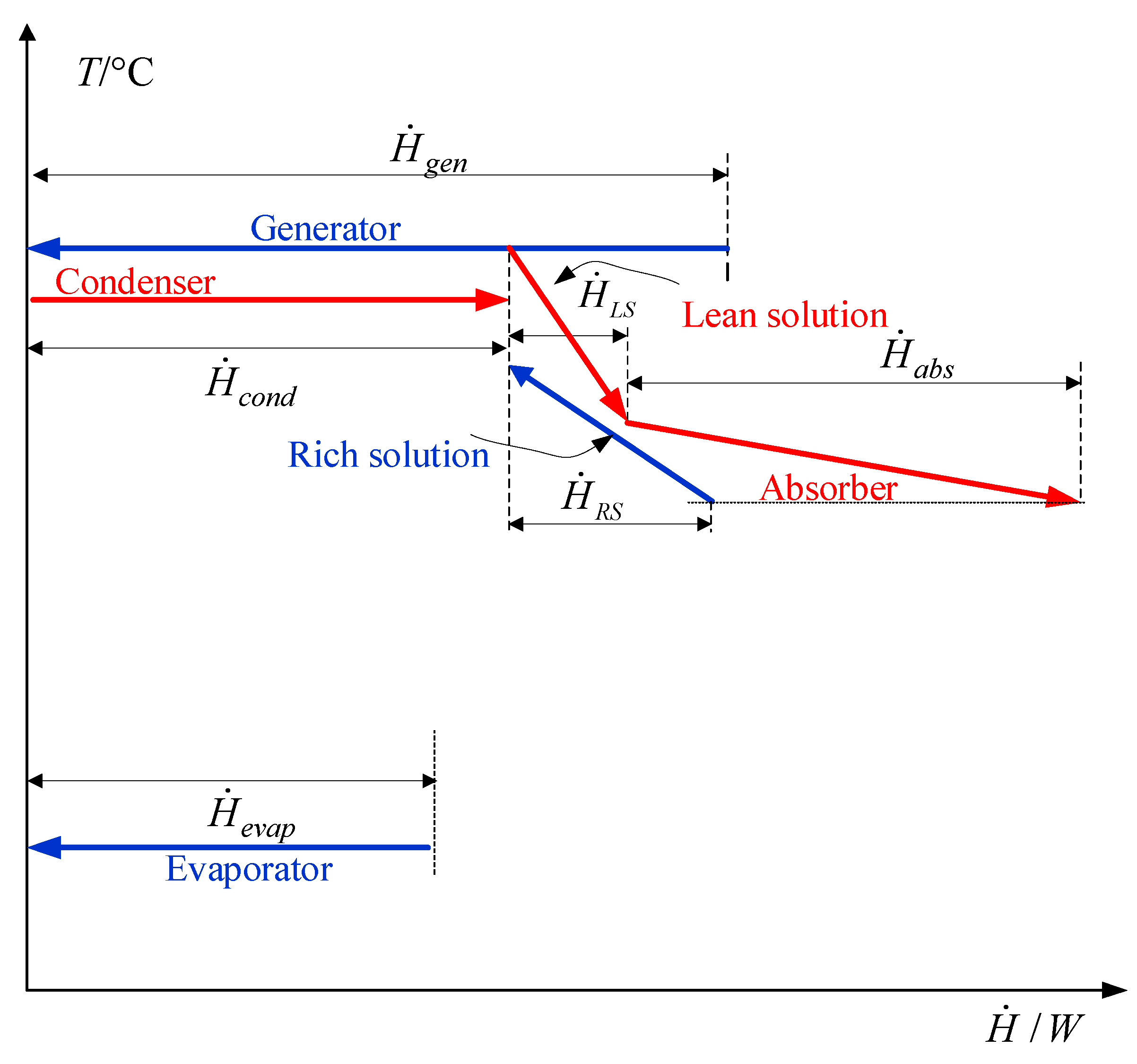
2.2.6. Overall Representation of Absorption Chilling

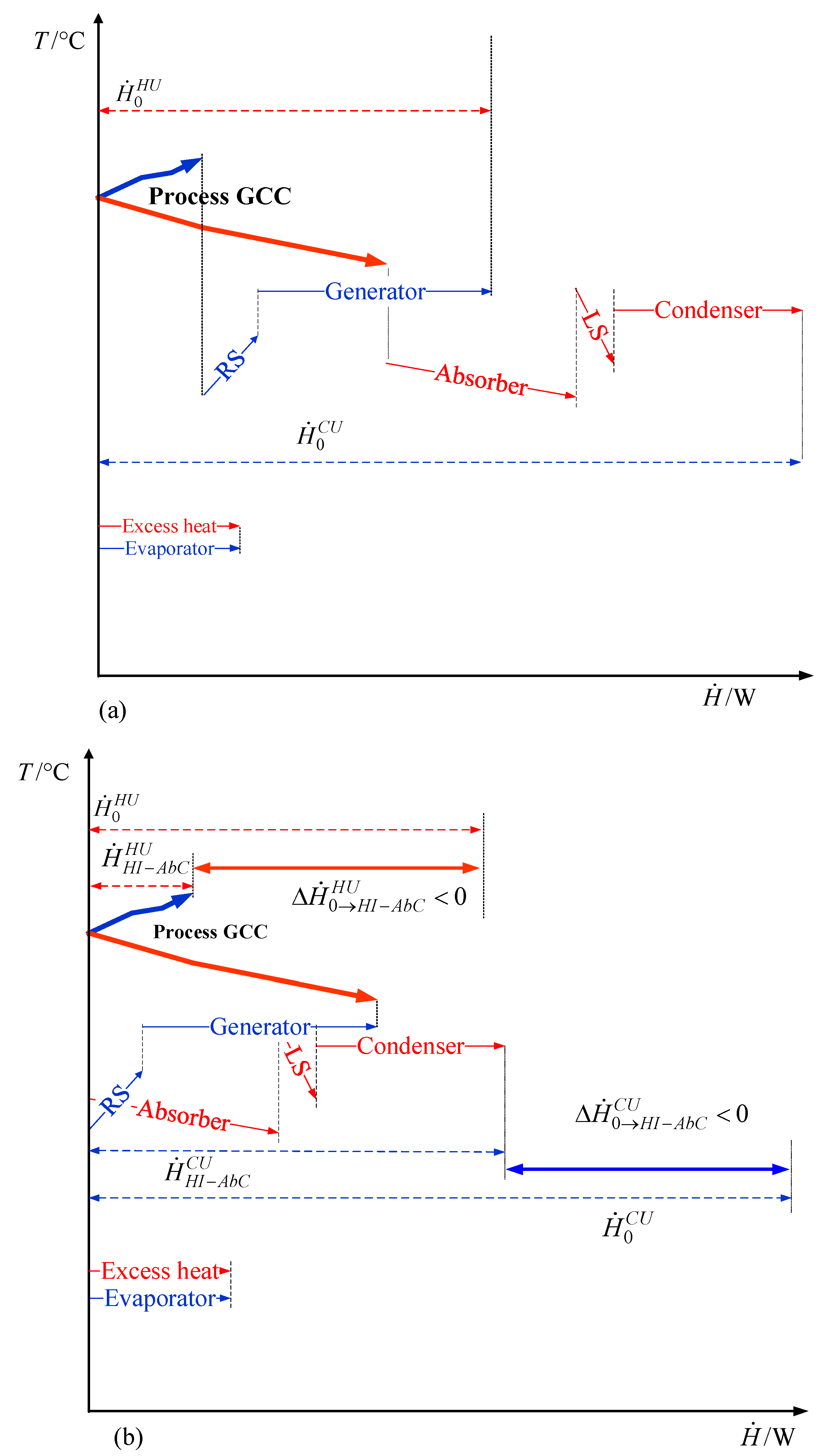
The overall representation of AC is given in Figure 7. It consists of the refrigerant, rich solution, and generator stream as cold streams, while condensation, absorption, and the lean solution stream are also shown as cold streams. The inlet temperature of the lean solution is equal to the temperature of the generator stream. The outlet temperature of the lean solution is equal to the inlet temperature of the absorption. The outlet temperature of the absorption is equal to the inlet temperature of the rich solution.

3. Integration of AC with a Process Using Pinch Analysis

Integration of AC with the process can be done by PA. PA is a thermodynamic method for improving energy efficiency through heat integration—matching of hot and cold streams with the aim of setting a target minimum consumption of hot and cold utility at a selected average minimum temperature difference. The GCC represents the total hot and cold utility demand in terms of quantity and temperature level. In this methodology, the Heat Recovery Pinch Point, or Pinch Point for short, represents a temperature above which there is only hot utility demand (heat sink), while below that temperature there is only cold utility demand (heat source). The integration of AC with the process can be performed after the streams representing AC have been identified.

The most convenient way is to overlay the derived streams with the GCC of the process and integrate them. The refrigeration requirement is already covered by the introduction of AC and is therefore not considered in the further integration. It should also be noted that the evaporator is an integral part of AC. It is therefore shown in the figures but not included in the integration analysis. Three different options for integrating AC with a process are discussed, namely (i) above the Pinch, (ii) below the Pinch, and (c) across the Pinch.

3.1. Integration above the Pinch

The full integration of AC above the Pinch is only hypothetical, since cooling above the Pinch, like any cooling, is forbidden. There would be no benefit to integrating AC fully above the Pinch. The heating and cooling requirements would be the same as if the AC operated alone.

3.2. Integration across the Pinch

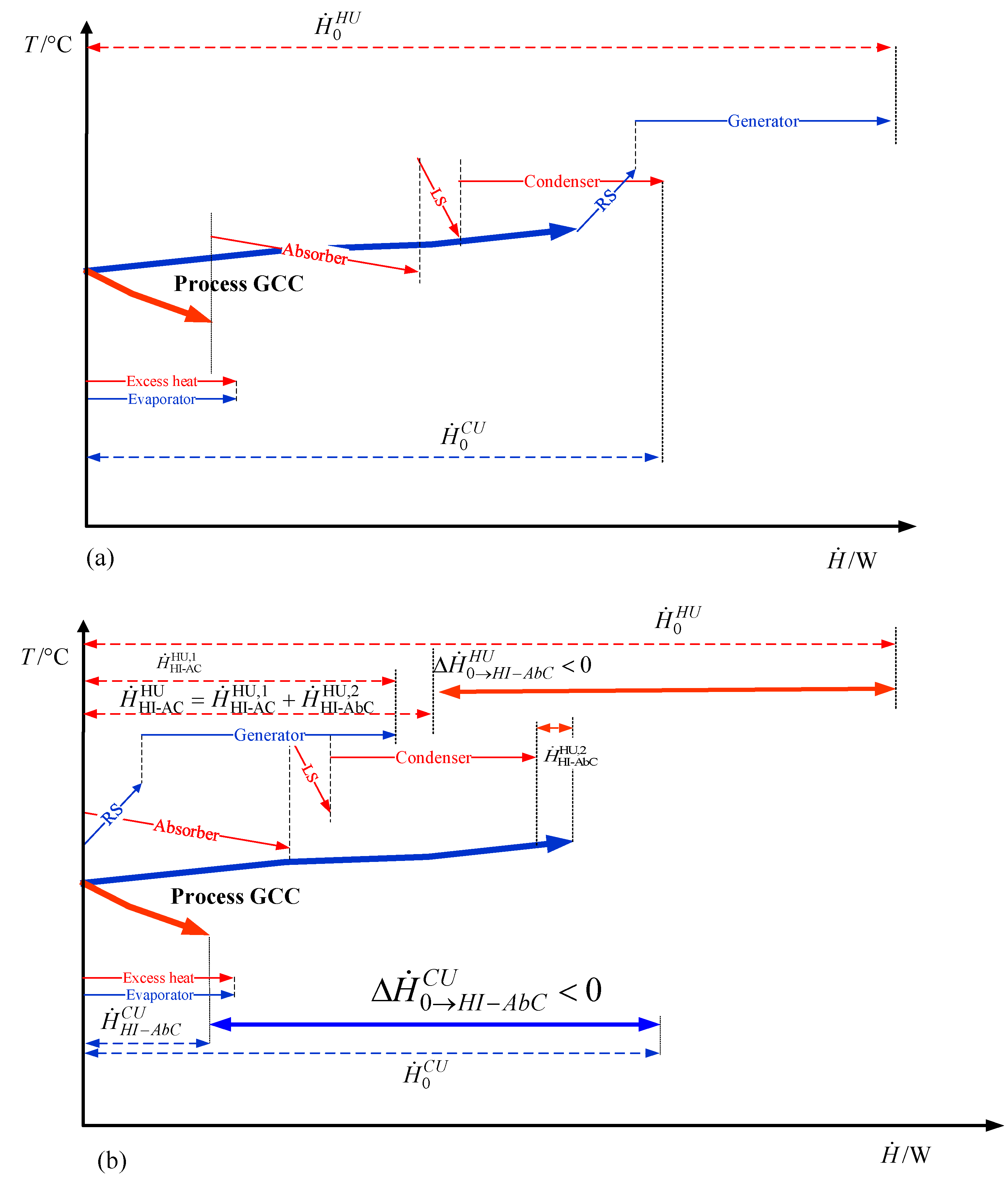
The integration of AC across the Pinch when heated for the generation of a refrigerant is supplied and all the heat from the AC is rejected above the Pinch, which is presented in Figure 8. As can be seen, the external utility is utilized for the generator and for heating the rich solution of the AC, while the condenser, absorber, and lean solution have a surplus of heat. The heat for the generator and rich solution can also be supplied from the hot process streams, if available, and the hot utility could be used for heating the cold process streams at higher temperatures. Since the heat from the refrigeration in the evaporator is “pumped” above the Pinch, the sum of heat surplus released from the AC above the Pinch is higher than the heat used for the generator and rich solution. Consequently, the consumption of external hot utility is decreased. As the AC is now performing the refrigeration, the consumption of external cold utility consumption is decreased as well. Therefore, it is advantageous to place the AC across the Pinch, so that the heat from the AC is removed entirely above the Pinch.

If the AC is integrated across the Pinch (Figure 9), so that most of the heat from the AC is dissipated below the Pinch, or if the process heat sink is small compared to the heat dissipated from the AC, the integration is poor. In this case, there is no benefit in integrating AC with the process as the consumption of both utilities remains the same as in the non-integrated case. Therefore, such integration across the Pinch is not advantageous.

3.3. Integration below the Pinch

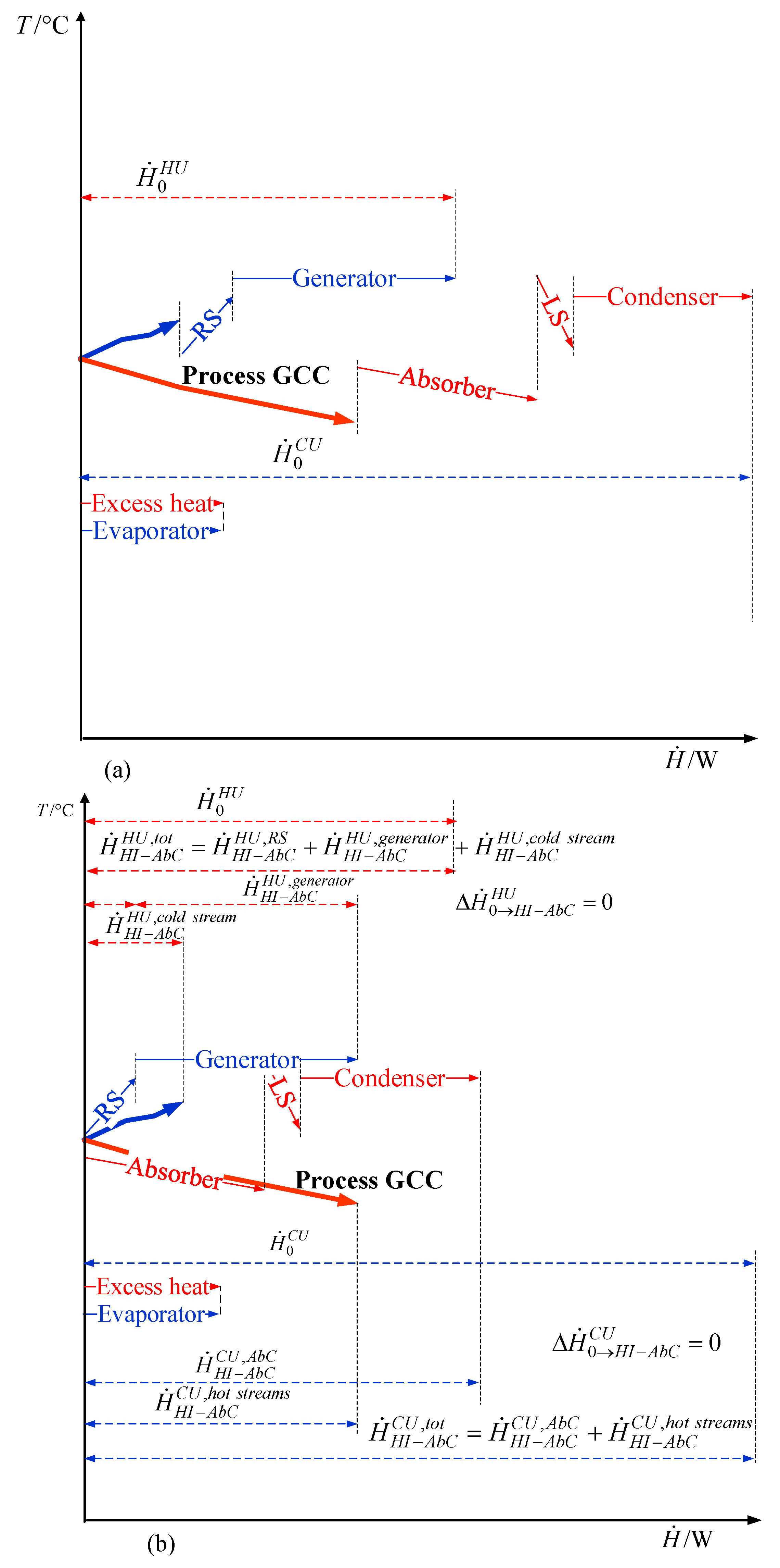
The integration of the AC below the Pinch Point is shown in Figure 10. As can be seen in this case, the consumption of hot utility is reduced as the heat demand of the rich solution and the generator is covered by the excess heat from the process (below the Pinch). For the same reason, cold utility consumption is also reduced. However, the excess heat from the absorber, lean solution, and condenser still need to be cooled by utilization of cold utility. Therefore, integrating AC below Pinch is reasonable, as both hot and cold utility consumptions are reduced.

3.4. Overall View of AC Integration with Process

Note that the combination of generator and condenser together with the absorber mimics a heat engine. It uses heat at a higher temperature and releases it at a lower one. On the other hand, the evaporator and absorber together with the condenser mimic a heat pump, where the heat at the lower temperature is consumed at the lower temperature, and by the work of the heat engine (generator + absorber, condenser) the heat is released at a higher temperature. Therefore, the highest utility reduction is achieved when the “heat engine” part is integrated above the Pinch and the “heat pump” part of the AC is integrated across the Pinch. A very good option for integration is also below the Pinch, as it takes advantage of the “heat engine” part of AC, while the “heat pump” part of AC remains neutral regarding hot and cold utility consumption.

4. Case Studies

The presented method for integration was tested by means of illustrative case studies. Two cases were tested: in one case, the integration was performed below the Pinch; in the other, all the heat was dissipated above the Pinch. In both cases, the cooling requirement was 1000 kW at 2 °C.

4.1. Case Study 1

The first case study presents an example of the integration of the AC below the Pinch Point. The input data for the process are presented in Table 1, while the parameters describing the AC are presented in Table 2. The derived streams from the AC can be seen in Table 3.

Note that utility consumption for the process alone was 2610 kW of hot utility and 5520 kW of cold utility, and for AC alone the generator and rich solution required 1116 kW of hot utility and the cooling of absorber, condenser, and lean solution needed 2115 kW of cold utility, giving a combined total consumption of 3720 kW of hot utility consumption and 7635 kW of cold utility for a nonintegrated case (Table 4). In the integrated case, the total hot utility consumption was reduced to 2610 kW, as the heat duty of the generator and the rich solution was covered by the excess process heat representing 1116 kW. The cold utility consumption was reduced by the same amount of heat, as the process cooling was partly covered by the heat requirement of AC. In this way, AC operates with a complete (100%) reduction of external hot utility and the reduction of total utility consumption corresponds to 30% for hot utility and 16% for cold utility.

Figure 11 presents the integration of the AC for case study 1. It is an example of when the AC is integrated entirely below the Pinch Point. As can be seen, it leads to lower cold utility consumption of the process by the heat needed for the generator (1116 kW).

4.2. Case Study 2

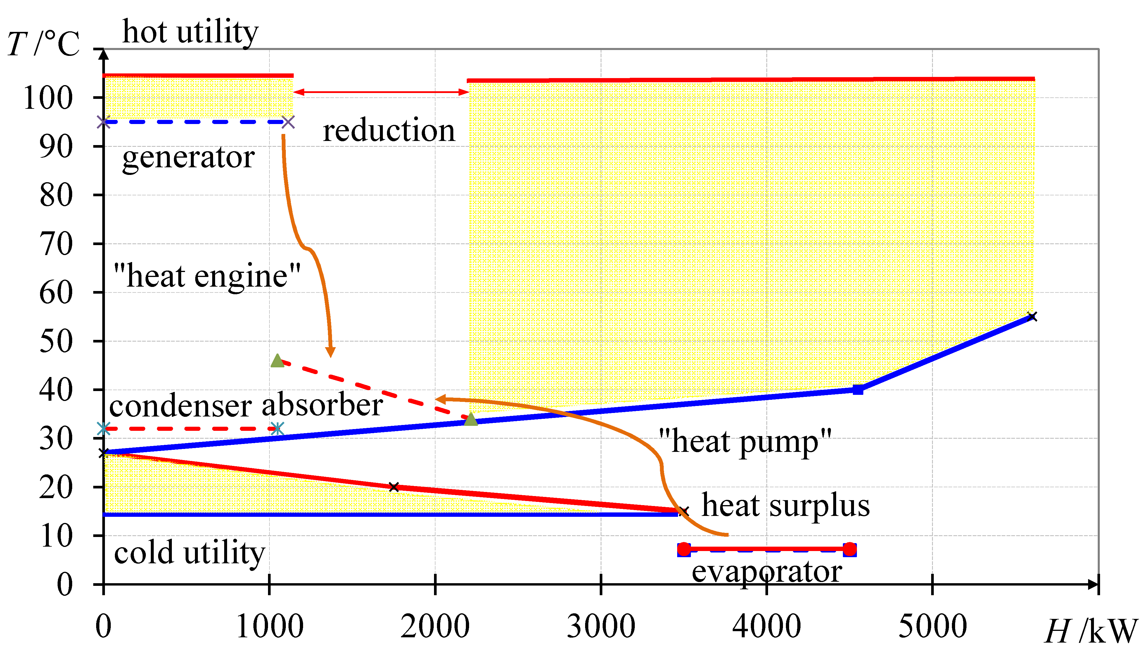
Case study 2 presents the integration of the AC across the Pinch, illustrating the combined effect of the heat pump and heat engine for the case of an AC. In this case study, the consumption of utilities for the process alone (Table 5) was 5600 kW for the hot utility and 3500 kW for the cold utility. For the AC alone (Table 6), the generator and rich solution would require 1238 kW of hot utility, and the cooling of absorber, condenser, and lean solution require 2238 kW. The total utility consumption for a non-integrated case was 6838 kW for the hot utility and 5768 kW for the cold utility. Table 7 presents the derived streams for AC.

The comparison of the non-integrated and integrated cases is present in Table 8. As can be seen, the integration of the AC across the Pinch led to the complete (100%) reduction of external hot and cold utilities to operate AC plus the partial reduction of hot utility for process due to pumping heat (1000 kW) through AC from below to above the Pinch. The corresponding reduction of total combined utility consumption was 33% for hot utility and 39% for cold utility.

The integration of the AC with the process is presented in Figure 12. It is evident that the generator still requires hot utility for its operation; however, it releases the same amount of the heat to the process heat sink above the Pinch with no net consumption of the external hot utility to operate AC. In addition, the hot utility consumption of the process is reduced by the effect of heat pump pumping the heat of the refrigeration from below to above the Pinch and given it off by the absorber and condenser. The reduction in the hot utility of the process thus corresponds to the pumped 1000 kW heat and the reduction in the total hot utility requirement corresponds to the sum of the heat given off by the condenser, absorber, and lean solution above the Pinch. Since the aforementioned units no longer need to be cooled, the cooling demand is reduced by the same amount. The cold utility requirement of the process remains the same in the integrated and non-integrated cases.

5. Conclusions

In heat integration, the AC can be represented as a combination of a heat engine and a heat pump. The main function of the heat engine is to use the heat at a higher temperature, convert it partially into work, and release the remaining heat at a lower temperature. On the other hand, the main function of a heat pump is to use part of the work to raise the temperature of the heat. In the AC heat pump, the heat is used to generate the work required to recover the refrigerant in the generator, while the remaining heat is rejected from the absorber, condenser, and lean solution. In this work, it is used to pump the heat from the refrigerator to higher temperature, rejecting it from the absorber, condenser, and lean solution.

The concept also supports the results obtained by studying the placement of the AC against the Pinch Point. Similar to heat engines, it is advantageous to integrate the AC across the Pinch, so that its “heat engine” is entirely above the Pinch, where both the supply of heat for the generator and the removal of heat above the Pinch occur. Similar to heat pumps, it is advantageous to locate the AC’s “heat pump” across the Pinch, where evaporation occurs below, and removal of the pumped heat occurs above the Pinch. Thus, integrating the AC across the Pinch Point has the dual benefit of reducing both heating and cooling consumption. Placing the AC below the Pinch Point is still beneficial because some of the excess heat below the pinch point that would otherwise be wasted is used to regenerate the refrigerant. Placing the AC above the Pinch, when the heat from the AC cannot be released or used above the Pinch, or placing the AC completely above the Pinch, is not practical, because in these cases, the demand for both heating and cooling energy would increase as if no heat integration had been performed.

Author Contributions

Conceptualization, A.N., Z.K. and M.B.; methodology, A.N. and Z.K.; writing—original draft preparation, A.N.; writing—review and editing, A.N., Z.K. and M.B.; visualization, A.N. All authors have read and agreed to the published version of the manuscript.

Funding

This research was funded by the Ministry of Education, Science and Sport of the Republic of Slovenia (OP20.03535) and the Slovenian Research Agency (P2-0414, J7-1816).

Institutional Review Board Statement

Not applicable.

Informed Consent Statement

Not applicable.

Data Availability Statement

Not applicable.

Conflicts of Interest

The authors declare no conflict of interest.

Nomenclature

Parameters
A, B	parameters for describing the relationship between pressure and temperature at certain compositions of NH₃ and H₂O
a, m, n	coefficients for heuristic calculations of temperature, specific heat, composition, etc.
$p_{abs}$	absorber pressure, Pa
$T^{evap}$	evaporation temperature, K
$x_{{NH}_{3}}^{ref}$	mole fraction of NH₃ in the refrigerant liquid phase
$x_{{NH}_{3}}^{RS}$	mole fraction of NH₃ in the rich solution
$x_{{NH}_{3}}^{LS}$	mole fraction of NH₃ in the lean solution
$w_{{NH}_{3}}^{LS}$	mass fraction of NH₃ in the lean solution
$w_{{NH}_{3}}^{RS}$	mass fraction of NH₃ in the rich solution
G	gravity, 9.81 m/s²
Variables
H	differential head, m
${\dot{H}}_{evap}$	enthalpy flow of evaporation, W
${\dot{H}}_{abs}$	enthalpy flow of absorption, W
${\dot{H}}_{preheat}^{ref, vap}$	enthalpy flow of preheating refrigerant from the evaporation outlet to the absorption inlet, W
${\dot{H}}_{abs}^{cool}$	enthalpy flow of cooling requirement (heat excess), W
${\dot{H}}_{gen}$	enthalpy flow of heat supplied to the generator, W
${\dot{H}}_{cond}$	enthalpy flow in the condenser, W
${\dot{H}}_{cond}^{R, liq}$	enthalpy flow in the liquid refrigerant in the condenser, W
${\dot{H}}_{evap}^{R, liq}$	enthalpy flow in the liquid refrigerant in the evaporator, W
${\dot{H}}_{evap}^{R, vap, in}$	enthalpy flow in the vapor refrigerant in the evaporator, W
$h_{T^{evap}}^{R, vap}$	specific heat of vapor at temperature of evaluation and certain refrigerant composition, J/g
$h_{T^{evap}}^{R, liq}$	specific heat of liquid at temperature of evaluation and certain refrigerant composition, J/g
$h_{T_{abs}^{in}}^{LS}$	specific heat of the lean solution at the absorber inlet temperature, J/g
$h_{T_{abs}^{out}}^{R S}$	specific heat of the rich solution at the absorber outlet temperature, J/g
$h_{T_{abs}^{out}}^{R, vap}$	specific heat of the refrigerant vapor at the absorber outlet temperature, J/g
$h_{T_{gen}^{reb}}^{LS}$	specific heat of the lean solution at the reboiler temperature $T_{gen}^{reb}$ , J/g
$h_{T^{cond}}^{R, vap}$	specific heat of the vapor of the refrigerant at the condenser temperature, J/g
$h_{T^{cond}}^{R, liq}$	specific heat of the liquid state of the refrigerant at $T^{cond}$ , J/g
$h_{T_{gen}^{feed}}^{RS}$	specific heat of the rich solution, at the feed temperature to the generator $T_{gen}^{feed}$ , J/g
P	shaft power of the pump, W
$p^{evap}$	evaporation pressure, Pa
$p^{gen}$	pressure in the generator, Pa
$q_{m, evap}^{R, vap, out}$	mass flowrate of the vapor at the outlet of the evaporator, g/s
$q_{m, evap}^{R, liq, in}$	mass flowrate of the liquid refrigerant at the inlet of the evaporator, g/s
$q_{m, evap}^{R, vap, in}$	mass flowrate of the vapor refrigerant at the inlet of the evaporator, g/s
$q_{m, cond}^{R, vap}$	mass flowrate of the vapor refrigerant in the condenser, g/s
$q_{m, cond}^{R, liq}$	mass flowrate of the liquid refrigerant in the condenser, g/s
$q_{m}^{LS}$	mass flowrate of the lean solution (liquid), g/s
$q_{m}^{RS}$	mass flowrate of the rich solution (liquid), g/s
$q_{m}^{R}$	mass flowrate of the refrigerant, g/s
SG	specific gravity of the fluid
$T_{p_{abs}, x^{RS}}^{RS}$	saturation temperature of rich solution at absorber pressure p_abs and certain molar fraction of NH₃ of the rich solution $x_{{NH}_{3}}^{RS}$ , K
$T_{abs}^{in}$	inlet temperature to the absorber, K
$T_{abs}^{out}$	outlet temperature from the absorber, K
$T^{cond}$	temperature of the condensation, K
$T_{gen}^{feed}$	feed temperature to the generator, K
$T_{gen}^{reb}$	reboiler temperature of the generator, K
$y_{p_{abs}, x_{{NH}_{3}}^{RS}}^{R}$	refrigerant molar fraction in the absorption
$ρ^{RS}$	density of the rich solution, g/m³
$ρ_{c}$	density at the critical point, g/m³
$ρ_{L}$	density of the pure liquid, g/m³
$τ$	reduced temperature complement to unity
$θ$	reduced temperature
Abbreviations
AC	Absorption chilling
PA	Pinch Analysis
GCC	Grand Composite Curve

Appendix A

Appendix A.1. Evaporator

The mass flowrate of the vapor at the outlet of the evaporator

q_{m, evap, out}^{R, vap, out}

is in balance with the mass flowrate of the liquid refrigerant

q_{m, evap}^{R, liq, in}

and refrigerant vapor

q_{m, evap}^{R, vap, in}

at the inlet of the evaporator.

q_{m, evap}^{R, vap, out} = q_{m, evap}^{R, liq} + q_{m, evap}^{R, vap, in}

(A1)

The amount of enthalpy flow of evaporation

{\dot{H}}_{evap}

is usually given by the refrigeration requirement. It can be determined by multiplication of the mass flowrate of liquid refrigerant

q_{m, evap}^{R, liq, in}

and the enthalpy difference between the specific heat of vapor

h_{T^{evap}}^{R, vap}

and liquid

h_{T^{evap}}^{R, liq}

at a certain temperature of evaporation. Thus, the mass flowrate of liquid refrigerant in the evaporator can be determined from Equation (A2).

{\dot{H}}_{evap} = q_{m, evap}^{R, liq} \cdot (h_{T^{evap}}^{R, vap} - h_{T^{evap}}^{R, liq})

(A2)

The temperature requirement T^evap of the evaporation process is also usually given by the refrigeration requirement. The required pressure p can be estimated from Equation (A3) (Sun, 1996) assuming a saturated mixture.

\log p^{evap} = A - \frac{B}{T^{evap}}

(A3)

The A and B are coefficients determined from Equations (A4) and (A5). The mole fraction of NH₃ in the refrigerant liquid phase

x_{{NH}_{3}}^{ref}

needs to be estimated for this purpose. It is assumed that the composition of the refrigerant in the liquid phase is similar to the one in the gas phase. This assumption can be made as the refrigerant is composed almost entirely of NH₃.

A = 7.44 - 1.767 \cdot x_{{NH}_{3}}^{ref} + 0.9823 \cdot {(x_{{NH}_{3}}^{ref})}^{2} + 0.3627 \cdot {(x_{{NH}_{3}}^{ref})}^{3},

(A4)

B = 2013.8 - 2155.7 \cdot x_{{NH}_{3}}^{ref} + 1540.9 \cdot {(x_{{NH}_{3}}^{ref})}^{2} - 194.7 \cdot {(x_{{NH}_{3}}^{ref})}^{3}

(A5)

Appendix A.2. Absorber

The mass balance of the absorber is presented in Equation (A6), indicating that sum of the mass balance of the lean solution

q_{m}^{LS}

and refrigerant

q_{m, evap, out}^{R, vap, out}

is in balance with the mass flowrate of the rich solution

q_{m}^{RS}

.

q_{m}^{LS} + q_{m, evap, out}^{R, vap, out} = q_{m}^{RS}

(A6)

The mass flow rate of the solution could be determined from the composition of both solutions. It should be noted that the molar fraction is, here, converted to mass fraction. The mass flowrate of only NH₃ can be determined from Equation (A7).

q_{m}^{LS} \cdot w_{{NH}_{3}}^{LS} + q_{m, evap, out}^{R, vap, out} \cdot w_{{NH}_{3}}^{LS} = q_{m}^{RS} \cdot w_{{NH}_{3}}^{RS}

(A7)

Equations (A6) and (A7) present a system of two equations with two unknowns, therefore, the mass flow rates of lean and rich solutions could be determined.

The absorption is assumed to be an isobaric process, and, despite the exothermic nature of absorption, it has a decreasing temperature, due to the higher temperature of the saturation of the lean solution compared to the rich solution. Therefore, a temperature decrease is necessary in order to obtain the required solubility at a certain pressure. The equilibrium temperature for the rich solution is presented in Equation (A8), while the lean solution calculation is made from Equation (A9). The coefficients of Equations (A8) and (A9) are presented in section Appendix A.7.

T_{p_{abs}, x_{{NH}_{3}}^{SS}}^{RS} = T_{0} \cdot \sum_{i = 1}^{14} a_{i} \cdot {(1 - x_{{NH}_{3}}^{RS})}^{m_{i}} \cdot {(\ln (\frac{p_{0}}{p_{abs}}))}^{n_{i}}

(A8)

T_{p_{abs}, x^{LS}}^{LS} = T_{0} \cdot \sum_{i = 1}^{14} a_{i} \cdot {(1 - x_{{NH}_{3}}^{LS})}^{m_{i}} \cdot {(\ln (\frac{p_{0}}{p_{abs}}))}^{n_{i}}

(A9)

The temperature of the lean solution, determined at the selected composition and selected pressure, was assumed to be the inlet temperature to the absorber

T_{abs}^{in}

, while, the temperature of the rich solution, at the same pressure and different composition, was the outlet temperature from the absorber

T_{abs}^{out}

. The amount of enthalpy flow released during absorption

{\dot{H}}_{abs}

can be determined as the sum of the specific heat of the lean solution at the absorber inlet temperature

h_{T_{abs}^{in}}^{LS}

multiplied by the mass flowrate of the lean solution

q_{m}^{LS}

, plus the specific heat of the refrigerant vapor at the absorber outlet temperature

h_{T_{abs}^{out}}^{R, vap}

multiplied by the mass flowrate of refrigerant

q_{m}^{R}

, subtracted by the specific heat of the rich solution at the absorber temperature

h_{T_{abs}^{out}}^{RS}

multiplied by the mass flowrate of the rich solution

q_{m}^{RS}

(Equation (A10)).

{\dot{H}}_{abs} = q_{m}^{LS} \cdot h_{T_{abs}^{in}}^{LS} + q_{m, evap}^{R, vap, out} \cdot h_{T_{abs}^{out}}^{R, vap} - q_{m}^{RS} \cdot h_{T_{abs}^{out}}^{RS}

(A10)

There is a pressure difference between the evaporation process and the absorption process. The pressure gradient is assumed to be covered by the sub-pressure created by the absorption process as the refrigeration vapor is dissolved in the lean solution. The temperature of the refrigerant is also increased. A part of the heat produced at absorption is utilized for these changes. The enthalpy flow of refrigerant preheating is determined as the difference between the specific enthalpy of vapor at the temperature of the absorber outlet and at the evaporation multiplied by the mass flowrate (Equation (A11)).

{\dot{H}}_{preheat}^{ref, vap} = q_{m, evap}^{R, vap, out} \cdot (h_{T_{abs}^{out}}^{R, vap} - h_{T^{evap}}^{R, vap})

(A11)

Therefore, the enthalpy flow of cooling requirement (heat excess) is the difference between the enthalpy flow of heat produced by absorption, reduced by that utilized for preheating.

{\dot{H}}_{abs}^{cool} = {\dot{H}}_{abs} - {\dot{H}}_{preheat}^{ref, vap}

(A12)

The relationship between the molar fraction of NH₃ in the vapor refrigerant and liquid phase in the rich solution can be described by the following Equation (A13). The coefficients for Equation (A13) are presented in section Appendix A.7.

y_{p_{abs}, x_{{NH}_{3}}^{RS}}^{R} = 1 - \exp [\ln (1 - x_{{NH}_{3}}^{RS}) {\sum_{i = 1}^{14} a_{i} (\frac{p_{abs}}{p_{0}})}^{m_{i}} {(x_{{NH}_{3}}^{RS})}^{n_{i} / 3}]

(A13)

Appendix A.3. Generator

The enthalpy flow requirement of the generator is determined from the heat and mass balances of the unit. In the generator, the rich solution mass flow

q_{m}^{RS}

is the sum of the mass flowrate of the lean solution

q_{m}^{LS}

and the mass flowrate of the refrigerant

q_{m, cond}^{R, vap}

(Equation (A14)).

q_{m}^{RS} = q_{m}^{LS} + q_{m, cond}^{R, vap}

(A14)

The purpose of the generator is to produce a refrigerant with a certain composition. This composition can be determined from Equation (A15) and should be similar to that obtained in the absorption process by Equation (A13).

y_{p_{gen}, x_{{NH}_{3}}^{LS}}^{R} = 1 - \exp [\ln (1 - x_{{NH}_{3}}^{LS}) {\sum_{i = 1}^{14} a_{i} (\frac{p_{gen}}{p_{0}})}^{m_{i}} {(x_{{NH}_{3}}^{LS})}^{n_{i} / 3}]

(A15)

At a certain temperature of the refrigerant outlet temperature from the generator, the required pressure is determined, in order to ensure the selected temperature is the temperature of saturation. For this purpose

\log p^{gen} = A - \frac{B}{T^{cond}}

(A16)

The A and B are coefficients determined from Equations (A17) and (A18). For this purpose, the mole fraction of NH₃ in the refrigerant liquid phase x is assumed to be similar to the vapor phase at the outlet (top) of the generator, as the content of the NH₃ is very high.

A = 7.44 - 1.767 \cdot x_{{NH}_{3}}^{ref} + 0.9823 \cdot {(x_{{NH}_{3}}^{ref})}^{2} + 0.3627 \cdot {(x_{{NH}_{3}}^{ref})}^{3}

(A17)

B = 2013.8 - 2155.7 \cdot x_{{NH}_{3}}^{ref} + 1540.9 \cdot {(x_{{NH}_{3}}^{ref})}^{2} - 194.7 \cdot {(x_{{NH}_{3}}^{ref})}^{3}

(A18)

The generator is, similarly to the absorber, assumed as an isobaric process. The feed temperature to the generator

T_{gen}^{feed}

is determined as the saturation temperature of the rich solution at the selected composition of the rich solution and the determined refrigerant pressure outlet. The reboiler temperature of the generator

T_{gen}^{reb}

is determined as the temperature of the lean solution at the selected composition and calculated pressure. The coefficients for Equations (A19) and (A20) are presented in section Appendix A.7.

T_{gen}^{feed} = T_{p_{gen}, x^{RS}}^{RS} = T_{0} \cdot \sum_{i = 1}^{14} a_{i} \cdot {(1 - x_{{NH}_{3}}^{RS})}^{m_{i}} \cdot {(\ln (\frac{p_{0}}{p_{gen}}))}^{n_{i}}

(A19)

T_{geb}^{reb} = T_{p_{gen}, x^{LS}}^{LS} = T_{0} \cdot \sum_{i = 1}^{14} a_{i} \cdot {(1 - x_{{NH}_{3}}^{WS})}^{m_{i}} \cdot {(\ln (\frac{p_{0}}{p_{gen}}))}^{n_{i}}

(A20)

The enthalpy balance is presented by Equation (A20). The enthalpy flow of generator

{\dot{H}}_{gen}

is the sum of the specific heat of the lean solution

h_{T_{gen}^{reb}}^{LS}

, at the reboiler temperature

T_{gen}^{reb}

, multiplied by the mass flowrate

q_{m}^{LS}

, plus the specific heat of vapor of the refrigerant

h_{T^{cond}}^{R, vap}

, at condenser temperature, multiplied by the mass flowrate

q_{m}^{R}

, subtracted by the specific heat of the rich solution

h_{T_{gen}^{feed}}^{RS}

, at the feed temperature to the generator

T_{gen}^{feed}

, multiplied by the mass flowrate

q_{m}^{RS}

.

{\dot{H}}_{gen} = q_{m}^{LS} \cdot h_{T_{gen}^{reb}}^{spec, RS} + q_{m, cond}^{R, vap} \cdot h_{T^{cond}}^{spec, vap} - q_{m}^{RS} \cdot h_{T_{gen}^{feed}}^{spec, RS}

(A21)

Appendix A.4. Condenser

The inlet vapor

q_{m, cond}^{R, vap}

and outlet liquid

q_{m, cond}^{R, liq}

mass flowrate at the condenser are equal (Equation (A22)).

q_{m, cond}^{R, vap} = q_{m, cond}^{R, liq}

(A22)

The condensation process was assumed to be isothermal at T^cond. It is the same selected temperature as used in the generator balance calculations. The enthalpy flow

{\dot{H}}_{cond}

in the condenser is calculated as the difference between the specific heat of the vapor and liquid state of the refrigerant at T^cond multiplied with the mass flowrate.

{\dot{H}}_{cond} = q_{m, cond}^{R, vap} \cdot (h_{T^{cond}}^{R, vap} - h_{T^{cond}}^{R, liq})

(A23)

Appendix A.5. Throttle Valve

A process of adiabatic expansion is performed by the throttle valve in order to reduce the temperature and pressure of the refrigerant to the required level for refrigeration. Within the process of cooling a certain amount of liquid refrigerant is evaporated, therefore, the mass flowrate of the liquid refrigerant passed from the condenser

q_{m, cond}^{R, liq}

is equal to the sum of the mass flowrate of liquid refrigerant

q_{m, evap}^{R, liq}

and mass flowrate of the vapor refrigerant

q_{m, evap}^{R, vap}

both at the evaporator inlet.

q_{m, cond}^{R, liq} = q_{m, evap}^{R, liq} + q_{m, evap}^{R, vap}

(A24)

The mass flow rate of the vapor refrigerant after expansion in the throttle valve can be determined by the enthalpy balance, as the process is adiabatic.

{\dot{H}}_{cond}^{R, liq} = {\dot{H}}_{evap}^{R, liq} + {\dot{H}}_{evap}^{R, vap, in}

(A25)

q_{m, cond}^{R, liq} \cdot h_{T_{cond}}^{R, liq} = q_{m, evap}^{R, liq} \cdot h_{T^{evap}}^{R, liq} + q_{m, evap}^{R, vap} \cdot h_{T^{evap}}^{R, vap}

(A26)

By combining Equations (A24) and (A26) the mass flow rate of evaporated refrigerant during the process of adiabatic expansion can be determined from Equation (A27).

q_{m, cond}^{R, liq} = \frac{h_{T^{evap}}^{R, vap} - h_{T^{cond}}^{R, liq}}{h_{T^{evap}}^{R, vap} - h_{T^{evap}}^{R, liq}} \cdot q_{m, evap}^{R, liq}

(A27)

Appendix A.6. Pump

The pump should be considered in order to increase pressure in the rich solution leaving the absorber that is pumped to the generator. The density of the media pumped should be estimated, in order to evaluate the power required for the pump (Equation (A28)). It is estimated as described in [21], where the liquid mixture is calculated as for a quasi-ideal mixture.

ρ^{RS} = x_{{NH}_{3}}^{RS} \cdot ρ_{{NH}_{3}, T_{{NH}_{3}}^{*}}^{RS} + (1 - x_{{NH}_{3}}^{RS}) \cdot ρ_{H_{2} O, T_{H_{2} O}^{*}}^{RS} + Δ ρ_{T_{m}^{\otimes}, x}

(A28)

The last term of the right-hand side of Equation (A28) is determined from Equation (A29).

Δ ρ_{T_{m}^{\otimes}, x} = (x_{{NH}_{3}}^{RS} (1 - x_{{NH}_{3}}^{RS}) - A \cdot {(x_{{NH}_{3}}^{RS})}^{2} (1 - x_{{NH}_{3}}^{RS})) ρ_{{NH}_{3}, T_{{NH}_{3}}^{*}}^{0.5} \cdot ρ_{{NH}_{3}, T_{{NH}_{3}}^{*}}^{0.5}

(A29)

In order to determine the “excess” density from an ideal one, the temperature

T_{m, x}^{\otimes}

should be determined by Equation (A30) in order to determine coefficient A as described in Equation (A31).

T_{m, x}^{\otimes} = \frac{T_{abs}^{out}}{T_{{c, H}_{2} O}}

(A30)

A = \sum_{i = 0}^{2} A_{1, i} \cdot {(T_{m, x}^{\otimes})}^{i} + \frac{\sum_{i = 0}^{2} A_{2, i} \cdot {(T_{m, x}^{\otimes})}^{i}}{x_{{NH}_{3}}^{RS}}

(A31)

where, A_1,i and A_2,i are the parameters presented in Table A1.

Table A1. Parameters for Equation (A31).

Stream	0	1	2
A₁	−2.41	8.31	−6.924
A₂	2.118	−4.05	4.443

The density of separate components could be estimated from Equation (A32).

\frac{ρ_{L}}{ρ_{c}} = \sum_{i = 0}^{6} A_{i} \cdot τ^{b_{i}}

(A32)

where ρ_c is the density at the critical point, A_i and b_i are the parameters presented in Table A2 for NH_3, and Table A3 for H₂O, τ is determined from Equation (A33) and Equation (A34).

Table A2. Parameters A_i and b_i for Equation (A32) for NH₃.

I	A	B
0	1	0
1	2.024913	0.33
2	0.840497	0.67
3	0.301559	1.67
4	−0.20927	5.33
5	−74.6025	14.33
6	4089.793	23.33

Table A3. Parameters A_i and b_i for Equation (A32) for H₂O.

I	A	B
0	1	0
1	1.993772	0.33
2	1.098521	0.67
3	−0.50945	1.67
4	−1.76191	5.33
5	−44.9005	14.33
6	−723,692	36.67

τ = 1 - θ

(A33)

θ = \frac{T_{m}}{T_{c, m}} = \frac{T_{{NH}_{3}}^{*}}{T_{{c, NH}_{3}}} = \frac{T_{H_{2} O}^{*}}{T_{{c, H}_{2} O}}

(A34)

The critical temperature of the mixture should be determined, in order to be able to determine the density of the mixture.

T_{c, m} = \sum_{i = 0}^{4} a_{i} {(x_{{NH}_{3}}^{RS})}^{i}

(A35)

where a_i is a parameter presented in Table A4.

Table A4. Parameter a_i for Equation (A35).

I	0	1	2	3	4
a_i	647.14	−199.822371	109.035522	−239.626217	88.689691

The pump capacity could be determined as can be seen in Equation (A36) [22], by multiplication of the mass flowrate

q_{m}^{RS}

with gravity g and differential head h divided by the pump’s efficiency

η

.

P = \frac{q_{m}^{RS} \cdot g \cdot h}{η}

(A36)

The differential head is determined from the pressure difference divided by the specific gravity SG of the fluid Equation (A37) [23].

h = \frac{10.197 \cdot Δ p}{S G}

(A37)

In Equation (A38) the calculated density of the solution is required, in order to determine the specific gravity SG [24].

S G = \frac{ρ_{solution}}{ρ_{H_{2} O, 4 ° C}}

(A38)

Appendix A.7. Specific Heat, Temperature, Pressure and Composition Relationships of the Solution

The specific heat of the refrigerant can be obtained from the Thermodynamic Tables for ammonia, under the assumption that the refrigerator fraction is 1. However, it is quite unrealistic to expect that it would be possible to generate pure refrigerant. Therefore, the specific heat was applied to an ammonia-water mixture. Simple calculations for an ammonia-water cycle were presented in [3]. They proposed the following correlation for the specific heat of an ammonia-water mixture as a vapor (Equation (A39)), where h₀ = 1000 kJ/kg and T₀ = 324 K, Y is the ammonia molar fraction in the gas phase of the ammonia-water mixture, T is the temperature of the mixture, a, m and n are the coefficients presented in Table A5.

h_{T, y}^{spec, gas} = h_{0} \cdot {\sum_{i = 1}^{17} a_{i} (1 - \frac{T}{T_{0}})}^{m_{i}} {(1 - y)}^{n_{i} / 4}

(A39)

The specific heat of an ammonia-water solution can be obtained similarly, as suggested in [3], where X is the mole fraction of ammonia in the liquid phase, h₀ is 100 kJ/kg and T₀ is 273.16 K. The coefficients a_i, m_i, and n_i are presented in Table A6.

h_{T, x}^{spec, liq} = h_{0} \cdot {\sum_{i = 1}^{16} a_{i} (\frac{T}{T_{0}} - 1)}^{m_{i}} x^{n_{i}}

(A40)

Table A5. Coefficients for Equation (A39) [3].

I	m_i	n_i	a_i
1	0	0	1.28827
2	1	0	0.125247
3	2	0	−2.08748
4	3	0	2.17696
5	0	2	2.35687
6	1	2	−8.86987
7	2	2	10.2635
8	3	2	−2.3744
9	0	3	−6.70515
10	1	3	16.4508
11	2	3	−9.36849
12	0	4	8.42254
13	1	4	−8.58807
14	0	5	−2.77049
15	4	6	−0.961248
16	2	7	0.988009
17	1	10	0.308482

Table A6. Coefficients for Equation (A40) [3].

I	m_i	n_i	a_i
1	0	1	−7.6108
2	0	4	25.6905
3	0	8	−247.092
4	0	9	325.952
5	0	12	−158.854
6	0	14	61.9084
7	1	0	11.4314
8	1	1	1.18157
9	2	1	2.84179
10	3	3	7.41609
11	5	3	891.844
12	5	4	−1613.09
13	5	5	622.106
14	6	2	−207.588
15	6	4	−6.87393
16	8	0	3.50716

The equilibrium temperature of vapor

T_{p, y}^{vap}

at certain pressure p, when the mole fraction of NH₃ in the gas phase is y, T₀ is 100 K, p₀ is 2 MPa, the coefficients a_i, m_i, and n_i are presented in Table A7 (Equation (A39)).

T_{p, y}^{vap} = T_{0} \cdot \sum_{i = 1}^{17} a_{i} \cdot {(1 - y)}^{m_{i} / 4} \cdot {(\ln (\frac{p_{0}}{p}))}^{n_{i}}

(A41)

The equilibrium temperature of liquid

T_{p, x}^{liq}

at certain pressure p, when the mole fraction of NH₃ in the liquid phase is x, T₀ is 100 K, p₀ is 2 MPa, the coefficients a_i, m_i, and n_i are presented in Table A8 (Equation (A40)).

T_{p, x}^{liq} = T_{0} \cdot \sum_{i = 1}^{14} a_{i} \cdot {(1 - x)}^{m_{i}} \cdot {(\ln (\frac{p_{0}}{p}))}^{n_{i}}

(A42)

Table A7. Coefficients for Equation (A41) [3].

I	m_i	n_i	a_i
1	0	0	3.24004
2	0	1	−0.03959
3	0	2	0.043562
4	0	3	−0.00219
5	1	0	−1.43526
6	1	1	1.05256
7	1	2	−0.07193
8	2	0	12.2362
9	2	1	−2.24368
10	3	0	−20.178
11	3	1	1.10834
12	4	0	100.1454
13	4	2	0.644312
14	5	0	−2.21246
15	5	2	−0.75627
16	6	0	−1.35529
17	7	2	0.183541

Table A8. Coefficients for Equation (A42) [3].

I	m_i	n_i	a_i
1	0	0	3.22302
2	0	1	−0.38421
3	0	2	0.046097
4	0	3	0.003789
5	0	4	0.000136
6	1	0	0.487855
7	1	1	−0.12011
8	1	2	0.010615
9	2	3	−0.00053
10	4	0	7.85041
11	5	0	−11.5941
12	5	1	−0.05232
13	6	0	4.89596
14	13	1	0.042106

The relationship between the compositions of the gas phase, indicated as a mole fraction in the vapor phase

y_{p, x}^{vap}

considering pressure p and mole fraction of NH₃ in the liquid phase X, can be described by Equation (A41). The coefficients for Equation (A41) are presented in Table A9, while p₀ is 2 MPa.

y_{p, x}^{vap} = 1 - \exp [\ln (1 - x) {\sum_{i = 1}^{14} a_{i} (\frac{p}{p_{0}})}^{m_{i}} x^{n_{i} / 3}]

(A43)

Table A9. Coefficients for Equation (A43) [3].

I	m_i	n_i	a_i
1	0	0	19.802202
2	0	1	−11.809267
3	0	6	27.747998
4	0	7	−28.863428
5	1	0	−59.161661
6	2	1	578.091305
7	2	2	−6.217367
8	3	2	−3421.98402
9	4	3	11,940.3127
10	5	4	−24,541.3777
11	6	5	29,159.1865
12	7	6	−18,478.229
13	7	7	23.481943
14	8	7	4803.10617

References

Hammond, G.; Norman, J. Heat recovery opportunities in UK industry. Appl. Energy 2014, 116, 387–397. [Google Scholar] [CrossRef] [Green Version]
Oluleye, G.; Jobson, M.; Smith, R.; Perry, S.J. Evaluating the potential of process sites for waste heat recovery. Appl. Energy 2016, 161, 627–646. [Google Scholar] [CrossRef]
Pátek, J.; Klomfar, J. Simple functions for fast calculations of selected thermodynamic properties of the ammonia-water system. Int. J. Refrig. 1995, 18, 228–234. [Google Scholar] [CrossRef]
Sun, D.-W. Thermodynamic design data and optimum design maps for absorption refrigeration systems. Appl. Therm. Eng. 1997, 17, 211–221. [Google Scholar] [CrossRef]
Sun, D.-W. Comparison of the performances of NH₃-H₂O, NH₃-LiNO₃ and NH₃-NaSCN absorption refrigeration systems. Energy Convers. Manag. 1998, 39, 357–368. [Google Scholar] [CrossRef]
Jawahar, C.; Saravanan, R. Generator absorber heat exchange based absorption cycle—A review. Renew. Sustain. Energy Rev. 2010, 14, 2372–2382. [Google Scholar] [CrossRef]
Jawahar, C.; Raja, B.; Saravanan, R. Thermodynamic studies on NH₃-H₂O absorption cooling system using pinch point approach. Int. J. Refrig. 2010, 33, 1377–1385. [Google Scholar] [CrossRef]
Du, S.; Wang, R.; Xia, Z. Optimal ammonia water absorption refrigeration cycle with maximum internal heat recovery derived from pinch technology. Energy 2014, 68, 862–869. [Google Scholar] [CrossRef]
Haywood, A.; Sherbeck, J.; Phelan, P.; Varsamopoulos, G.; Gupta, S.K.S. Thermodynamic feasibility of harvesting data center waste heat to drive an absorption chiller. Energy Convers. Manag. 2012, 58, 26–34. [Google Scholar] [CrossRef]
Sayadi, Z.; Thameur, N.B.; Bourouis, M.; Bellagi, A. Performance optimization of solar driven small-cooled absorption-diffusion chiller working with light hydrocarbons. Energy Convers. Manag. 2013, 74, 299–307. [Google Scholar] [CrossRef]
Kim, D.; Ferreira, C.I. Air-cooled LiBr-water absorption chillers for solar air conditioning in extremely hot weathers. Energy Convers. Manag. 2009, 50, 1018–1025. [Google Scholar] [CrossRef]
Weber, C.; Berger, M.; Mehling, F.; Heinrich, A.; Núñez, T. Solar cooling with water-ammonia absorption chillers and concentrating solar collector—Operational experience. Int. J. Refrig. 2014, 39, 57–76. [Google Scholar] [CrossRef]
Ghaebi, H.; Karimkashi, S.; Saidi, M. Integration of an absorption chiller in a total CHP site for utilizing its cooling production potential based on R-curve concept. Int. J. Refrig. 2012, 35, 1384–1392. [Google Scholar] [CrossRef]
Nikbakhti, R.; Wang, X.; Hussein, A.K.; Iranmanesh, A. Absorption cooling systems—Review of various techniques for energy performance enhancement. Alex. Eng. J. 2020, 59, 707–738. [Google Scholar] [CrossRef]
Linnhoff, B.; Dunford, H.; Smith, R. Heat integration of distillation columns into overall processes. Chem. Eng. Sci. 1983, 38, 1175–1188. [Google Scholar] [CrossRef]
Townsend, D.W.; Linnhoff, B. Heat and power networks in process design. Part II: Design procedure for equipment selection and process matching. AIChE J. 1983, 29, 748–771. [Google Scholar] [CrossRef]
Glavič, P.; Kravanja, Z.; Homšak, M. Heat integration of reactors—I. Criteria for the placement of reactors into process flowsheet. Chem. Eng. Sci. 1988, 43, 593–608. [Google Scholar] [CrossRef]
Fu, C.; Gundersen, T. Integrating compressors into heat exchanger networks above ambient temperature. AIChE J. 2015, 61, 3770–3785. [Google Scholar] [CrossRef]
Fu, C.; Gundersen, T. Correct integration of compressors and expanders in above ambient heat exchanger networks. Energy 2016, 116, 1282–1293. [Google Scholar] [CrossRef]
Wan Alwi, S.R.; Lee, C.K.M.; Lee, K.Y.; Abd Manan, Z.; Fraser, D.M. Targeting the maximum heat recovery for systems with heat losses and heat gains. Energy Convers. Manag. 2014, 87, 1098–1106. [Google Scholar] [CrossRef]
M. Conde Engineering. Thermophysical Properties of {NH₃+H₂O} Mixtures for the Industrial Design of Absorption Refrigeration Equipment. Available online: www.mrc-eng.com/Downloads/NH3%26H2O%20%20Props%20English.pdf (accessed on 4 May 2016).
Engineering Toolbox. Calculate Pump Hydraulic and Shaft Power. Available online: www.engineeringtoolbox.com/pumps-power-d_505.html (accessed on 10 May 2016).
Engineering Toolbox. Converting Pump Heat to Pressure and Vice Versa. Available online: www.engineeringtoolbox.com/pump-head-pressure-d_663.html (accessed on 10 May 2016).
Engineering Toolbox. Density, Specific Weight and Specific Gravity. Available online: www.engineeringtoolbox.com/density-specific-weight-gravity-d_290.html (accessed on 10 May 2016).

Figure 1. (a) Basic process scheme and (b) pressure-temperature diagram of AC.

Figure 2. (a) Heat integration of cooling represented by the composite curve of the evaporator and (b) presentation of evaporator as a part of AC cycle.

Figure 3. (a) Heat integration of the absorption process presented by a composite curve and (b) presentation of absorber as a part of AC cycle.

Figure 4. Heat integration of (a) rich and (b) lean solution represented by composite curve and (c) presentation of both, rich and lean, as a part of AC cycle.

Figure 5. (a) Heat integration of generator represented by a composite curve and (b) presentation of generator as a part of AC cycle.

Figure 6. (a) Heat integration of a condenser by a composite curve and (b) presentation of condenser as a part of AC cycle.

Figure 7. Overall graphical presentation of the AC.

Figure 8. (a) Non-integrated and (b) integrated case of AC-process system-integrating AC across the Pinch Point, rejecting heat above the Pinch.

Figure 9. (a) Non-integrated and (b) integrated case of AC-process system when process heat demand is small.

Figure 10. (a) Non-integrated and (b) integrated case of AC with process-integrating AC below the Pinch.

Figure 11. Integration of the AC for the process as case study 1.

Figure 12. Integration of the AC with the process for case study 2.

Table 1. Input data for process streams for case study 1.

Stream	T^IN/°C	T^OUT/°C	CP/kW °C⁻¹
Hot 1	95	80	60
Hot 2	92	60	150
Cold 1	95	110	30
Cold 2	82	95	180

Table 2. Input data for the AC for case study 1.

$T^{evap} / ° C$	$y_{{NH}_{3}}^{vap}$	$T^{ref} / ° C$	${\dot{H}}^{evap} / kW$	$p^{abs} / bar$	$x_{{NH}_{3}}^{LS}$	$x_{{NH}_{3}}^{LS}$
2	0.99	17	1000	4.347	0.45	0.54

Table 3. Derived streams from the AC for case study 1.

Stream	T^IN/°C	T^OUT/°C	$\dot{H} / kW$
Evaporator	2	2	1000
Absorber	48	34	1083
Generator	63	63	1110
Condenser	17	17	1021
rich solution	34	49	6
lean solution	63	48	11

Table 4. Comparison of integrated and non-integrated solution for case study 1.

	${\dot{H}}^{HU} / kW$	${\dot{H}}^{AC, HU} / kW$	$Total {\dot{H}}^{HU} / kW$	${\dot{H}}^{CU} / kW$	${\dot{H}}^{AC, CU} / kW$	$Total {\dot{H}}^{CU} / kW$
Non-integrated	2610	1116	3726	5520	2115	7635
Integrated	2610	0	2610	4404	2115	6519
Difference		−1116	−1116	−1116		−1116
Difference			30%			16%

Table 5. Input data for the process streams for case study 2.

Stream	T^IN/°C	T^OUT/°C	CP/kW °C⁻¹
Hot 1	25	20	100
Hot 2	32	20	250
Cold 1	35	50	70
Cold 2	22	35	350

Table 6. Input data for the AC for case study 2.

$T^{evap} / ° C$	$y_{{NH}_{3}}^{vap}$	$T^{ref} / ° C$	${\dot{H}}^{evap} / kW$	$p^{abs} / bar$	$x_{{NH}_{3}}^{LS}$	$x_{{NH}_{3}}^{LS}$
2	0.99	37	1000	4.347	0.43	0.50

Table 7. Derived stream from the AC for case study 2.

Stream	T^IN/°C	T^OUT/°C	CP/kW
evaporator	2.0	2.0	1000
absorber	48	21	1166
generator	90	90	1112
condenser	17	17	1050
rich solution	21	35	126
lean solution	63	48	22

Table 8. Comparison of integrated and non-integrated solution for case study 2.

	${\dot{H}}^{HU} / kW$	${\dot{H}}^{AC, HU} / kW$	$Total {\dot{H}}^{HU} / kW$	${\dot{H}}^{CU} / kW$	${\dot{H}}^{AC, CU} / kW$	Total ${\dot{H}}^{CU} / kW$
Non-integrated	5600	1238	6838	3500	2238	5738
Integrated	4600	0	4600	3500	0	3500
Difference	−1000	−1238	−2238		−2238	−2238
Difference			33%			39%

Publisher’s Note: MDPI stays neutral with regard to jurisdictional claims in published maps and institutional affiliations.

© 2022 by the authors. Licensee MDPI, Basel, Switzerland. This article is an open access article distributed under the terms and conditions of the Creative Commons Attribution (CC BY) license (https://creativecommons.org/licenses/by/4.0/).

Share and Cite

MDPI and ACS Style

Nemet, A.; Kravanja, Z.; Bogataj, M. Integration of an Absorption Chiller to a Process Applying the Pinch Analysis Approach. Processes 2022, 10, 1028. https://0-doi-org.brum.beds.ac.uk/10.3390/pr10051028

AMA Style

Nemet A, Kravanja Z, Bogataj M. Integration of an Absorption Chiller to a Process Applying the Pinch Analysis Approach. Processes. 2022; 10(5):1028. https://0-doi-org.brum.beds.ac.uk/10.3390/pr10051028

Chicago/Turabian Style

Nemet, Andreja, Zdravko Kravanja, and Miloš Bogataj. 2022. "Integration of an Absorption Chiller to a Process Applying the Pinch Analysis Approach" Processes 10, no. 5: 1028. https://0-doi-org.brum.beds.ac.uk/10.3390/pr10051028

Note that from the first issue of 2016, this journal uses article numbers instead of page numbers. See further details here.

Article Menu

Integration of an Absorption Chiller to a Process Applying the Pinch Analysis Approach

Abstract

1. Introduction

2. Methods

2.1. Absorption Chilling

2.2. Deriving the Representative Streams for Each Unit of Absorption Chilling

2.2.1. Evaporator

2.2.2. Absorber

2.2.3. Rich and Lean Solutions

2.2.4. Generator

2.2.5. Condenser

2.2.6. Overall Representation of Absorption Chilling

3. Integration of AC with a Process Using Pinch Analysis

3.1. Integration above the Pinch

3.2. Integration across the Pinch

3.3. Integration below the Pinch

3.4. Overall View of AC Integration with Process

4. Case Studies

4.1. Case Study 1

4.2. Case Study 2

5. Conclusions

Author Contributions

Funding

Institutional Review Board Statement

Informed Consent Statement

Data Availability Statement

Conflicts of Interest

Nomenclature

Appendix A

Appendix A.1. Evaporator

Appendix A.2. Absorber

Appendix A.3. Generator

Appendix A.4. Condenser

Appendix A.5. Throttle Valve

Appendix A.6. Pump

Appendix A.7. Specific Heat, Temperature, Pressure and Composition Relationships of the Solution

References

Share and Cite

Article Metrics

Article Access Statistics

Further Information

Guidelines

MDPI Initiatives

Follow MDPI