
Estimation Parameters of Soil Solute Transport Processes by Using the Electric Resistivity Method


1
School of Water Conservancy & Environment Engineering, Zhejiang University of Water Resources and Electric Power, Hangzhou 310018, China
2
Key Laboratory for Technology in Rural Water Management of Zhejiang Province, Hangzhou 310018, China
*
Author to whom correspondence should be addressed.
Processes 2022, 10(5), 975; https://0-doi-org.brum.beds.ac.uk/10.3390/pr10050975
Submission received: 15 April 2022
/
Revised: 10 May 2022
/
Accepted: 10 May 2022
/
Published: 13 May 2022
(This article belongs to the Special Issue Processes of Pollution Control and Resource Utilization)
Abstract
:Preferential solute transport is a common phenomenon in soil, and it is of great significance to accurately describe the mechanism of pollutant transport and water and soil environmental governance. However, the description of preferential solutes still relies on applying solute breakthrough curves for model parameters fitting. At present, most of the solute breakthrough curves are obtained indoors, and with some limitations. Therefore, this study established a method for securing solute breakthrough curves based on the electrical resistivity method. The research results show that the change in soil concentration during the tracer infiltration process can be captured by establishing the fitting relationship between soil resistivity and solute concentration. Then the solute breakthrough curve can be found. Through a time moment analysis, the difference between the breakthrough curve parameters obtained by the traditional method and the resistivity method is slight; the average error is less than 10%. On this basis, the sensitive response of the parameters of the “mobile–immobile” model to concentration was elucidated through different concentration tracer experiments, among which β and D are more sensitive, and w is less sensitive. The suitable tracer concentration range should be 50–120 mg/L. Therefore, the established method could obtain the breakthrough curves and describe the transport of preferential solutes at the field scale.
1. Instruction
Preferential flow is a common phenomenon of water and solute transport in soil, and the pollutants it carries can reach deep soil and aquifers [1,2,3]. Due to the short interaction time between preferential water and solutes and the soil matrix, soil pollutants cannot be wholly absorbed and degraded by the soil matrix, thus increasing the risk of polluting groundwater and affecting biological growth and human health [4,5]. Therefore, the transport mechanism of solutes in soil with preferential channels is key to comprehensively revealing the soil solute pollution transportation process and then providing schemes to protect soil and water security [6,7].
Many scholars [8,9,10,11] have detailed research on the mass flow, diffusion, and chemical coupling in soil solute transport. The soil convection–diffusion equation (Convection Dispersion Equation) proposed by Nielson et al. [12,13,14,15,16] is widely used in the numerical simulation of solute transport. The equation could give a good description of convection and dispersion in the process of solute transport under homogeneous conditions. However, due to its limited interpretation of the early breakthrough and trailing phenomena in breakthrough curves (BTCs), the mobile–immobile water model (MIM) can improve the effectiveness of the CDE equation in the physical and chemical non-equilibrium description of the solute transport process [17,18,19].
However, both the CDE and the MIM need to use the breakthrough curves for parameter estimation. The breakthrough curves are generally measured by an indoor saturated soil column test, which will disturb the soil, thereby affecting the accuracy and limiting the acquisition of field-scale parameters [20,21,22,23]. Therefore, the current methods still have gaps in obtaining regional-scale soil solute transport parameters. At present, it is urgent to break through the limitations of soil solute parameter acquisition, to solve the problem that the existing preferential flow model is only suitable for indoor soil column research and lay the foundation for the regional-scale preferential flow solute transport simulation. However, high-density electrical resistivity tomography (ERT) is a non-destructive detection method that has recently become widely used in acquiring soil moisture and solute transport parameters due to its flexible detection scale and suitability for three-dimensional dynamic monitoring [24,25,26]. Many scholars [27,28,29] have used the method to study water and solute transport parameters in soil and achieved fruitful results, laying a theoretical foundation for acquiring soil-water parameters. However, there is still insufficient data to support the use of this method to obtain field BTCs.
Consequently, this study intends to use ERT to get unsaturated solute breakthrough curves with a specially designed lysimeter. The purpose is to carry out a tentative analysis of the solute breakthrough curves in the field. This will provide a new method for the acquisition of soil solute transport parameters at the regional scale, thus making it possible to accurately describe soil solute transport. Since it is a field method for obtaining soil solute transport parameters, and is not affected by soil physical properties, it can be applied to various soil types worldwide. At the same time, in order to evaluate the accuracy of the obtained parameters, the characteristics of the MIM’s parameters are intended to be studied to provide data support for the description of the field-scale solute transport in the preferential flow.
2. Experimental Theory and Methods
2.1. Device Design and Experimental Scheme
The undisturbed soil of this experiment was collected in the Changhua River Basin, which is located at the source of the Qiantang River in Zhejiang Province. The primary soil type was paddy soil, the average proportion of silt, clay, and sand were 45.35%, 38.61%, and 16.04 respectively, and the preferential flow was developed [30]. The basin belongs to the subtropical monsoon climate zone, with four distinct seasons and uniform distribution of precipitation seasons. The annual precipitation is between 800 m and 1600 m. The yearly average temperature in this area is 15.3 degrees, the average yearly evaporation is 1150 mm, and the average annual rainfall is 1703.01 mm. According to the investigation, the thickness of the vadose zone is about 100 cm. Therefore, this study selected the area with developed channels (0–100 cm) as the primary research area [31].
The experiment was completed in a self-designed special lysimeter. The design of the lysimeter is shown in Figure 1. It was a cube with a length, width, and height of 1 m. It was reinforced with steel rings, and stainless steel was installed on the four sides. Sixty-four electrodes were installed on each surface, with 256 electrodes for the entire cube. All electrodes were connected to an E60DN resistivity meter (Geopen, China) using copper wires to measure soil electric resistivity. The top of the cube soil column related to a constant water head device as the upper boundary for infiltration under different water head conditions. To minimize the disturbance to the undisturbed soil, the lysimeter was directly inserted into the undisturbed soil in the field. The surrounding area was excavated. Then, the bottom plate of the lysimeter was inserted to maintain the integrity of the soil core.
To obtain the breakthrough curve of the soil and its spatial variation characteristics, the soil core was conceptually divided into four parts in this study. Each piece was installed with soil moisture sensors (TDR100, CAMPBELL) at 20 cm, 40 cm, 60 cm, and 80 cm from the soil surface to the bottom for collecting the initial soil moisture. In addition, four small vacuum pumps were installed at the bottom of each part, and the lower boundary condition with a certain suction was set during the experiment. Four vacuum pumps controlled four areas respectively; the vacuum pump was connected to the collection bottles, then the collected solution volume, concentration, and other parameters were determined in the laboratory.
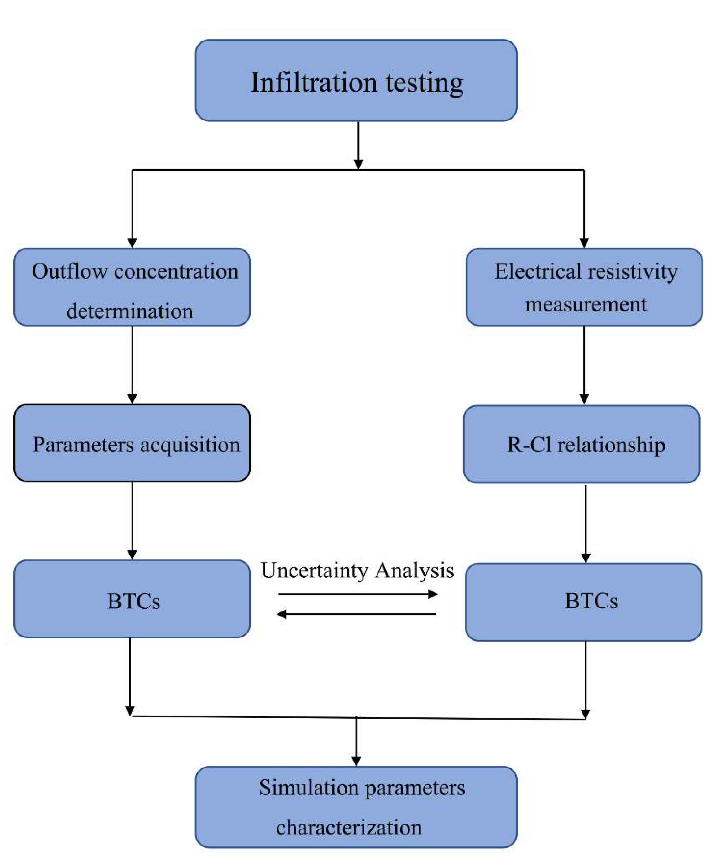
Soil samples were collected from the corresponding regions and brought back to the laboratory to obtain the soil’s physical parameters. The soil texture information is shown in Table 1 and was measured by laser particle sizer (S3500, Manufactured by Microtrac MRB). The soil texture differences in the four regions are apparent. The subregional parameter acquisition method can effectively capture the differences caused by soil heterogeneity, thereby laying a foundation for further description of soil preferential solute transport. The overall scheme of this experiment is shown in Figure 2, which is generally divided into two parts. The first part is establishing a BTCs acquisition scheme based on the electric resistivity method. During the solution infiltration test, the concentration and resistivity of the collected soil samples were measured and a relationship established to obtain BTCs. The other part is to collect solution samples through a specially designed vacuum pump device and use traditional methods to get BTCs. The primary purpose is to verify the feasibility of the established BTCs acquisition scheme based on the electrical resistivity method by comparing it with the traditional scheme. Consequently, the uncertainty analysis of the proposed project is carried out. The parameters of MIM are determined in terms of obtained BTCs, which provide theoretical support for the field application of the electric resistivity method to get the solute transport parameters of the vadose soil.
2.2. High-Density Electric Resistivity Tomography Method
As shown in Figure 1, the horizontal and vertical electrode distances were 14 cm; the electrodes were divided into eight columns on each face, 32 columns were engaged with the resistivity measurement using the dipole-dipole array; 62,496 measurements were conducted in total. To reduce the uncertainty of the measurement, the backward error analysis method was applied to estimate the error. By calculating the difference between the normal and back measurements, errors more significant than 15% were excluded from further calculation. Reasonable data were further calculated using the inversion method proposed by Lu et al. [32,33] to obtain the soil resistivity value. However, the process will not be discussed here due to space limitations. In addition, the resistivity of the soil samples was determined by the four-electrode method in the laboratory, and the chloride ion concentration was determined by the national standard method.
2.3. MIM Parameters Determination Using BTCs
The traditional convection–dispersion model cannot accurately describe the preferential flow. According to previous research, the “mobile–immobile model” (MIM) has certain advantages for describing soil solute transportation for preferential flow, which divides the soil into a moving water area (A) and a non-moving water area (B). There is no water exchange but solute diffusion between the two areas, and it only depends on the concentration difference between the two areas. Therefore, MIM was used to fit the obtained breakthrough curves. The dimensionless form of MIM can be described as [34]:
The initial condition is the given concentration boundary, and the upper boundary is:
The lower boundary is the fixed water head boundary in the above equations: C, Z, T are dimensionless concentration, depth, and time respectively; P is the peclet number; f is the proportion of the mobile water adsorption area; β is the proportion of the mobile water area; α is the mass exchange coefficient between the two areas; L is the length of the soil column; CA, CB are the dimensionless concentration values of the mobile water area and the immobile water area, respectively; kd is the adsorption coefficient; is the soil bulk density; Dm is the moving area dispersion coefficient; vm is the pore flow rate in the moving area; R is the resistance factor; v is the pore water flow rate; θ is the volumetric water content. There are D, P, R, β, and ω in the model that need to be fitted by BTCs. In this study, Levenberg–Marquart’s algorithm [35], widely used in nonlinear fitting, was used to fit the measured BTCs.
3. Results
3.1. Establishment of R-cl− Relationship
Determining the quantitative relationship between resistivity and tracer chloride ions is crucial for obtaining BTCs by the electrical resistivity method. In this study, samples were taken from four areas in the undisturbed soil core. The soil resistivity under different ion concentrations is measured in the laboratory, and the relationship was determined by the nonlinear fitting method. However, the initial water content of the soil has a significant impact on the relationship, so, referring to the actual initial water content of the soil, the resistivity and ion concentration under different initial water content was calibrated.
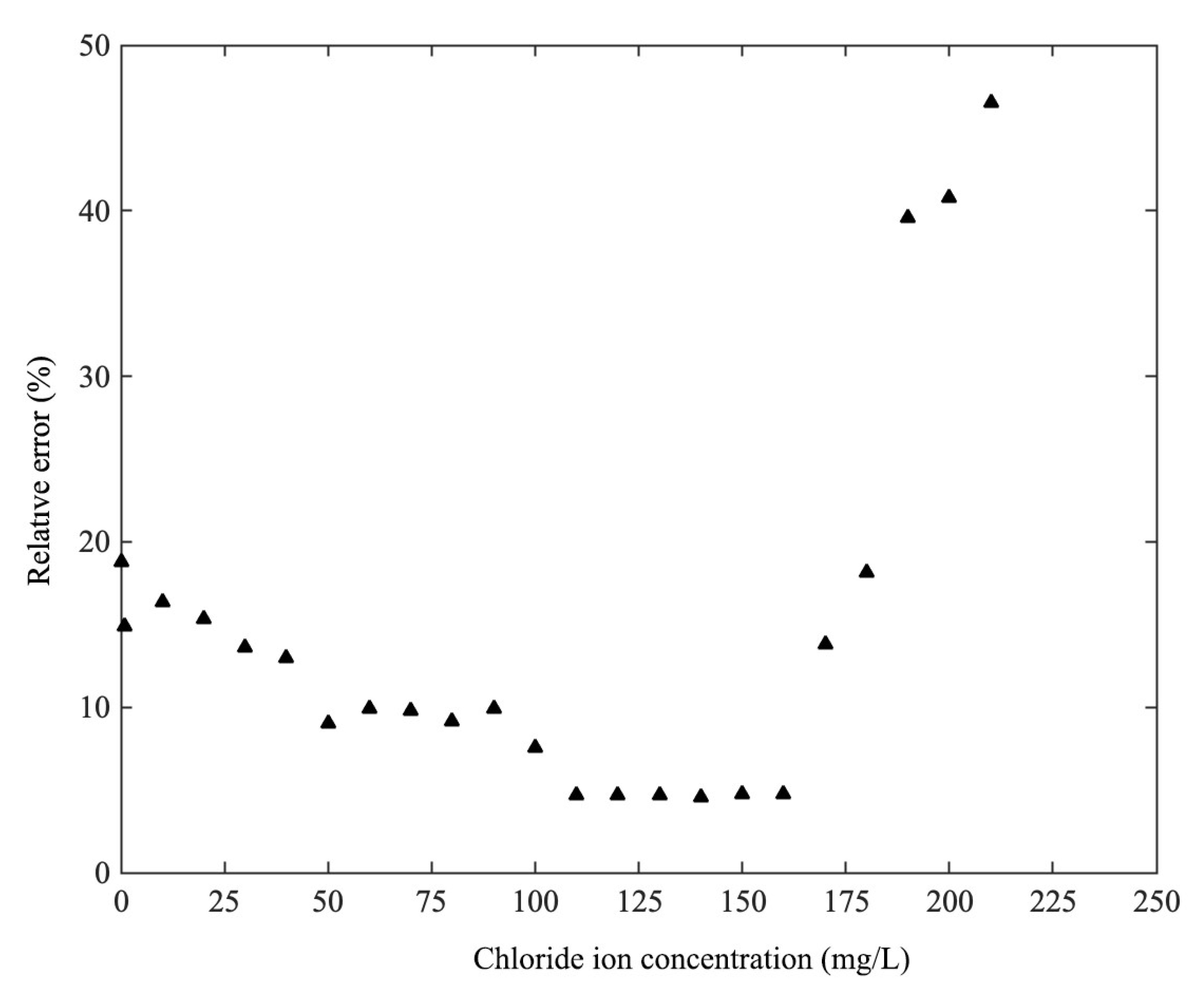
The initial soil content measured shows a small change. Figure 3 shows the calibrated relationship between resistivity and chloride ion concentration fitted by the power and exponential functions, respectively. According to the fitting results of the judgment parameter R2 and the Nash efficiency coefficient in Table 2, the power function is better than the exponential function. From the overall trend, the resistivity decreases with the increase of chloride ion concentration. This is because the electrical conductivity increases with the growth of chloride ions, which makes the resistivity tend to fall. In addition, due to the nonlinear relationship between resistivity and chloride ion concentration, the error distribution range based on the measured and simulated data was calculated. Figure 4 shows that when the chloride ion concentration is between 50–160 mg/L, the error between the measured value and the simulated value is small, less than 10%; when the ion concentration is less than 50 mg/L, the error is between 10–20%. However, when the ion concentration is greater than 160 mg/L, the relative error is significant, ranging from 20% to 60%. This is due to the error caused by the reduced sensitivity of the resistivity to high concentrations of chloride ions.
3.2. The Determination of the BTCs
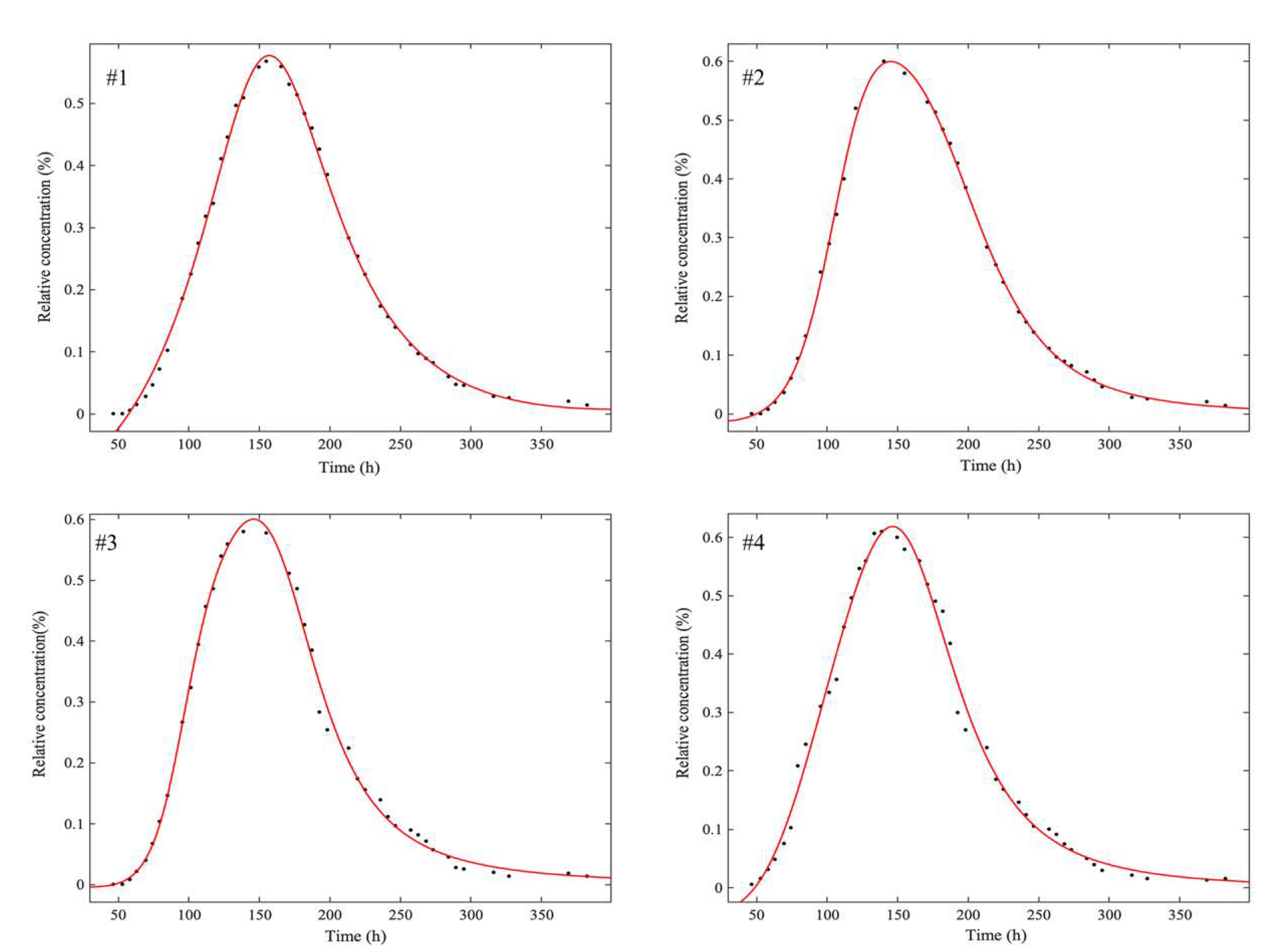
In this study, chloride ions with an initial concentration of 70 mg/L were used for infiltration experiments. According to the determined resistivity–chloride ion concentration relationship, the resistivity of the four regions of the soil column during the infiltration process was monitored, and the inversion calculation was carried out. The obtained resistivity value of each area at different times was converted to chloride ion concentration to estimate the breakthrough curve. Figure 5 shows the obtained BTCs for four regions determined by the ERT method. As shown, the MIM has a good fitting result for the breakthrough experimental data in which the correlation coefficients are greater than 0.9 while all R2 are above 0.8 in each site. Hence, the presented method could capture the front, peak, and tail features of the breakthrough process. Overall, the four regions show similar characteristics: single peak, asymmetry, and tailing. However, there are still some differences, such as the arrival time of peak concentration. The difference of peak concentration arrival time in sites 1, 3 and 4 is small, and site 2 reaches the peak concentration first. Thus, it can be inferred that there are preferential channels in the four regions, and certain heterogeneity happens in all sites. In addition, the BTCs concentration value obtained by the resistivity method is generally low, which may be due to the systematic nature of the resistivity measurement errors.
3.3. Parameter Characteristic Analysis of Breakthrough Curve
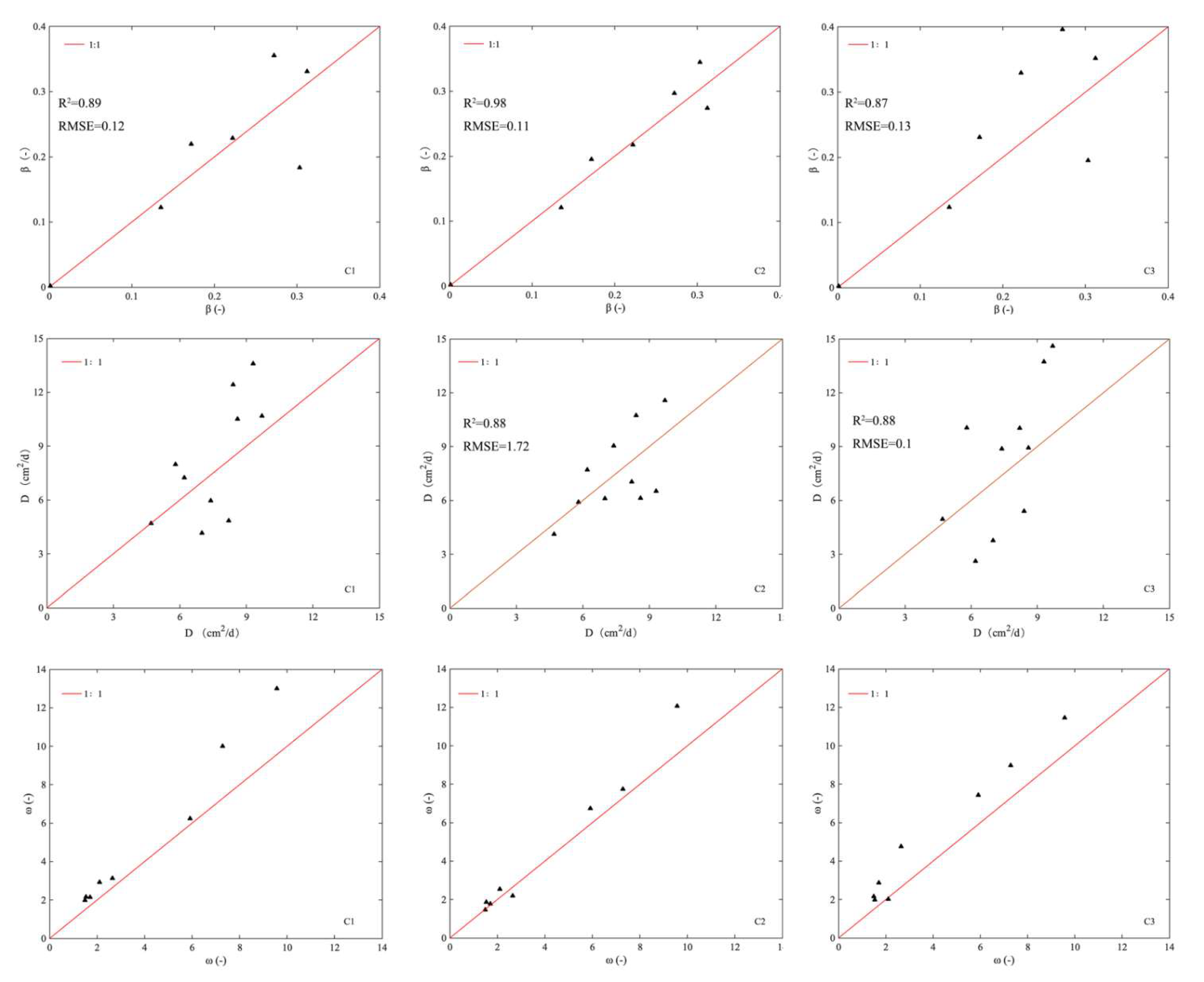
This study investigated the effect of different tracer concentrations on the fitting parameters of breakthrough curves. Figure 6 shows the dispersion parameters β, D, and w fitted by ERT and traditional methods at three different concentrations (concentration 1: 15 mg/L; concentration 2: 85 mg/L; concentration 3: 140 mg/L) respectively. The results show that parameter β is more sensitive to concentration, as the error of the low and medium concentration is relatively small, the R2 is a respective 0.89, 0.98, the RMSE is a respective 0.12, 0.11. The results also show that the data scatter degree is larger at the higher concentration, the R2 being 0.87 and the RMSE 0.13, where the parameter deviations obtained by the two methods were the smallest under the condition of medium concentration of tracer. This is caused by the difference in the sensitivity distribution of β to the concentration. The sensitivity of β is higher at medium and low concentrations, and the fitting value is relatively accurate.
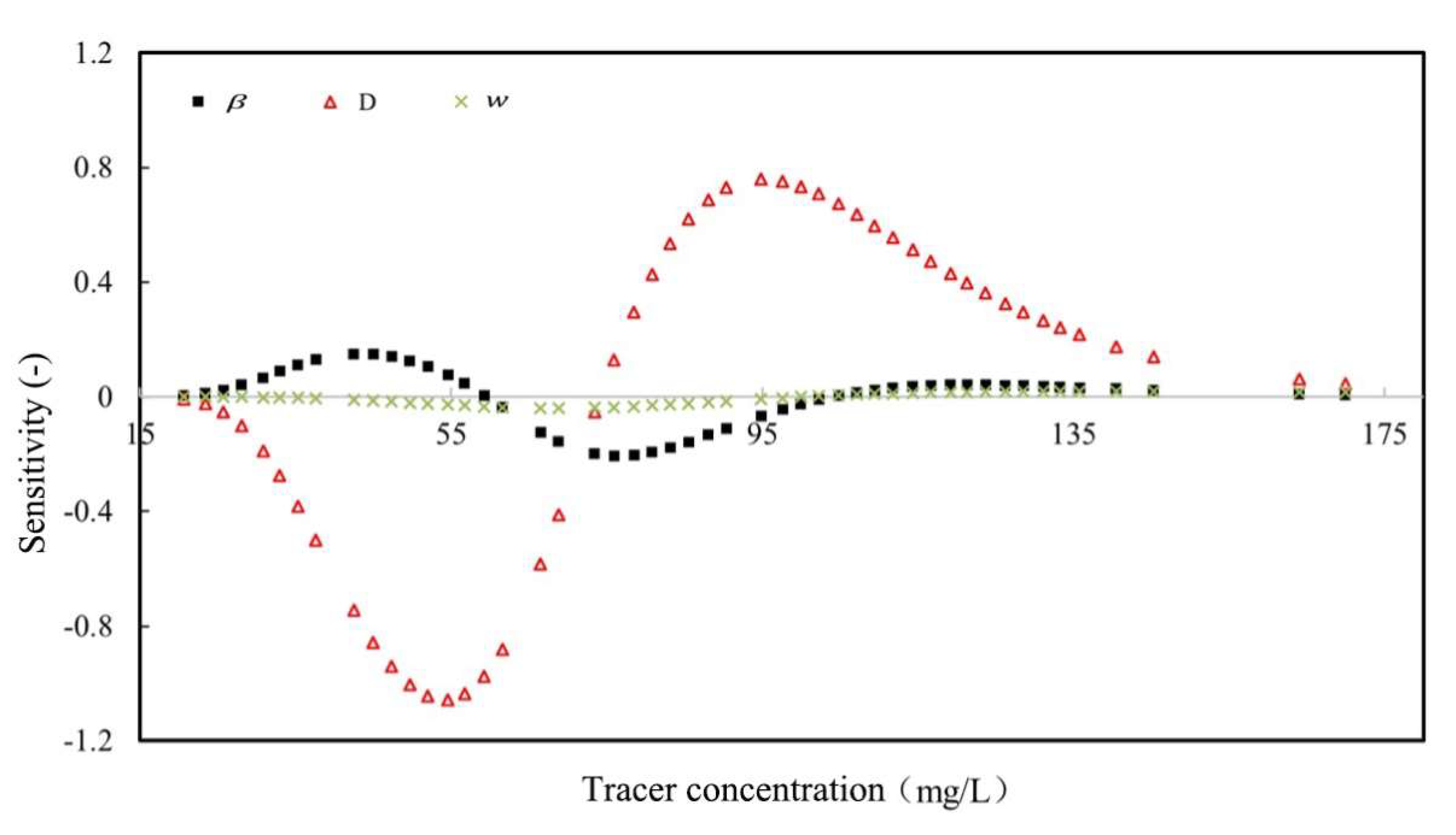
In contrast, the sensitivity to high concentration solutions is reduced, thus affecting the fitting accuracy. The dispersion D also showed similar variation characteristics, the most sensitive to concentration, with the most significant error at high concentration, with R2 of 0.86 and RMSE of 3.2. The low and medium concentration error was small, the medium concentration error was the smallest, and R2 was 0.92 with an RMSE of 1.72. The RMSE value of w at high concentration was 3.5, but the R2 values at three concentrations were more significant than 0.9, and the difference was slight. From the response results of the three parameters to the concentration, β and D were more sensitive to the change of concentration, and the sensitivity of medium and low concentrations was relatively high. w was less sensitive to changes in concentration, and the parameter fitting accuracy gap under different concentrations was small. According to the method proposed by [36], the sensitivity of parameters at different concentrations was calculated in this study, and the calculation results are shown in Figure 7. This result is also consistent with the results in Figure 6. D was the most sensitive to concentration, and the sensitivity value was the highest when the concentration was about 55 mg/L and 95 mg/L; β is the second; the most heightened sensitivity happens at concentrations around 35 mg/L and 70 mg/L; while the sensitivity of w to concentration ws poor which shows a slight difference with the change of concentration. This provides data support for selecting a reasonable concentration of tracer in the breakthrough curve acquisition experiment.
4. Discussion
Time moment analysis [37] is usually used to quantitatively describe the shape of BTCs and estimate solute transport parameters. This study used time moments to assess the gap between traditional and new methods. The time moment can be described as:
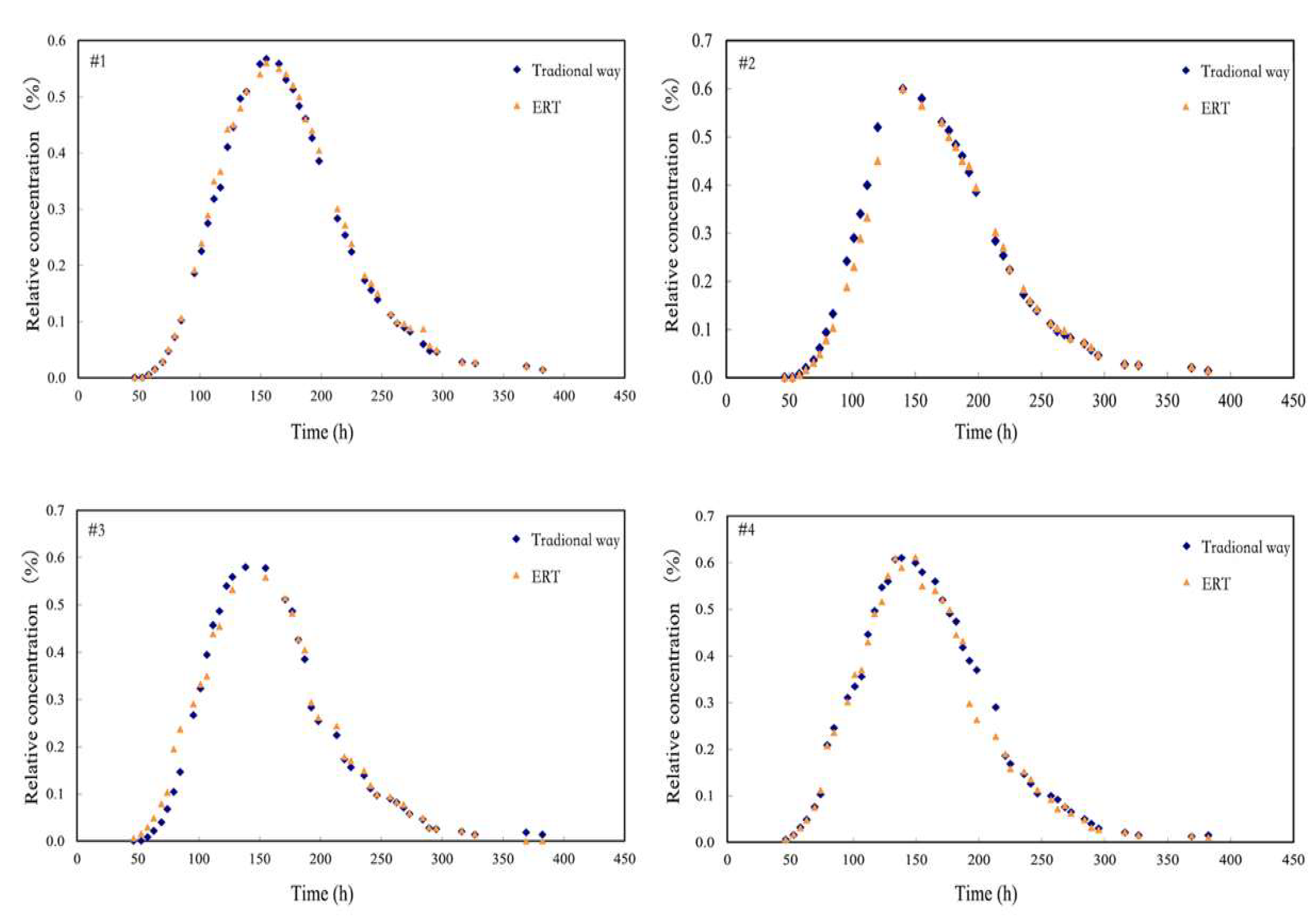
where Z is a dimensionless spatial coordinate; T is dimensionless time; C and C0 are solute concentration and input solute concentration respectively (M/L3); P is the order of the moment. Thus, the first-order standard moment represents the breakthrough time, the second-order center moment represents the average extension, while S represents the degree of symmetry of the breakthrough curve. In this study, time moments were used to calculate BTCs obtained by traditional methods [21] and ERT respectively, so as to obtain , , S. The soil breakthrough curves of different sites, obtained by using the traditional method and ERT, are shown in Figure 8. Table 3 presents the calculation results of the time moment of breakthrough curves for two different methods. From the value of S, which represents the degree of symmetry in Table 3, the variability of soil pores in No. 2 and No. 4 sites is higher than that in No. 1 and No. 3 sites.
It can be seen that the relative concentrations obtained in this series of experiments were all less than 1, which is more consistent with the results obtained by other scholars [38], mainly due to the presence of water in the soil, which has a specific dilution effect on the solution. Meanwhile, the measurement sensitivity is another contributor to the occurrence of low concentrations. Binley et al. [39] have pointed out that the low sensitivity of ERT away from the electrode led to the underestimation of the change of water, which they believed was the main reason for the mass balance error in the tracer experiment. However, in our experimental device design, we refer to the scheme of koestel et al. [40], so that the concentration deviation can be reduced to an acceptable range.
Compared with the traditional method, the first-order standard moment had an average error of 9.25%, a maximum error of 17%, and a minimum of 5%. The average error of the second-order central moment was 14.35%, the maximum error is 17.8%, and the minimum error was 9%; The average mistake of S was 5.4%, the maximum error was 10.6%, and the minimum error was 2.4%. The results show that the average errors were all less than 10%. The error of the coefficient S was the smallest, and the error of the second-order central moment was the largest, but the overall difference is negligible. According to previous studies [31], the more developed the macropores, the smaller the value of . Therefore, it can be inferred that the macropores in the No. 4 area were the most developed, and the breakthrough time was the shortest; the macropores in the No. 1 area were relatively less developed, and the breakthrough time was longer. represents the average extension of the curve; the more significant the value, the more advanced the macropores. The calculation results show that the value of in the No. 4 area was the largest. The preferential flow had a significant effect, which is highly consistent with the calculated value of .
In our experiment, it is found that the outflow concentration does not show a systematic change with the change of water supply head. This is similar to the conclusion obtained by Wehrer and Slater, [38]. Gomez et al. [41] has also pointed out that with the increase of water head, the development of finger flow may be increased, and the finger flow mainly moves laterally, which weakens the longitudinal flow and makes the resulting flow concentration show a decreasing trend. In addition, the relationship between resistivity and ion concentration established in this study adopts different fitting methods, so it is concluded that the fitting effect of power function is better, which is also confirmed by the research of Sheng et al. [42]. From the similar research carried out by relevant scholars [43,44,45], the fitting relationship between the two does not consider the physical mechanism in detail, which has a certain empirical nature. Therefore, more tests need to be carried out for different types of soil (water content, texture, and structure) in order to attempt different fitting schemes to establish a more accurate relationship between the two variables.
5. Conclusions
In this study, by establishing a fitting relationship between resistivity and tracer concentration, the concentration changes of soil tracer were captured, and the solute breakthrough curve was obtained. Results have shown that the relationship between resistivity and solute concentration is sensitive to concentration changes, and the appropriate concentration range should be 50–120 mg/L. The concentration fitting error outside this range is significant. Compared with the relevant parameters of the time moment, the solute breakthrough curve obtained by the ERT method has a small gap from the traditional method. There are differences in the sensitivity of the parameters of the “mobile–immobile model” to the concentration of the tracer, among which β and D are more sensitive. In contrast, the sensitivity of w is weaker, mainly caused by the difference in the sensitivity of different parameters to the concentration. A reasonable concentration range should be paid attention to.
Author Contributions
Conceptualization, D.L. and C.X.; methodology, Y.X.; software, N.G.; validation, J.Q. and H.W.; writing—original draft preparation, D.L.; writing—review and editing, C.X.; project administration, D.L. and C.X.; All authors have read and agreed to the published version of the manuscript.
Funding
This research was funded by [Zhejiang Public Welfare Technology Application Research Project] grant number [LGF21D020002]; [Key Technology Research and Development Program of Zhejiang] grant number [2021C03019]; [Zhejiang Natural Science Foundation] grant number [LZJWD22E090001]. And The APC was funded by [Key Technology Research and Development Program of Zhejiang].
Acknowledgments
The paper was supported by Zhejiang Public Welfare Technology Application Research Project [No. LGF21D020002] and Key Technology Research and Development Program of Zhejiang [No. 2021C03019] and Zhejiang Natural Science Foundation [No. LZJWD22E090001].
Conflicts of Interest
The authors declare no conflict of interest.
References
- Hyman, J.D. Flow channeling in fracture networks: Characterizing the effect of density on preferential flow path formation. Water Resour. Res. 2020, 56, e2020WR027986. [Google Scholar] [CrossRef]
- Jačka, L.; Walmsley, A.; Kovář, M.; Frouz, J. Effects of different tree species on infiltration and preferential flow in soils developing at a clayey spoil heap. Geoderma 2021, 403, 115372. [Google Scholar] [CrossRef]
- Nimmo, J.R. The processes of preferential flow in the unsaturated zone. Soil Sci. Soc. Am. J. 2021, 85, 1–27. [Google Scholar] [CrossRef]
- Mencaroni, M.; Morari, F.; Ferro, N.D. Shallow water table affects solute transport parameters in silty-loam soils. Geophys. Res. Abstr. 2019, 21, 1. [Google Scholar]
- Wang, X.; Li, Y.; Si, B.; Ren, X.; Chen, J. Simulation of Water Movement in Layered Water-Repellent Soils using HYDRUS-1D. Soil Sci. Soc. Am. J. 2018, 82, 1101–1112. [Google Scholar] [CrossRef]
- Cheng, Y.; Ying, Y.; Japip, S.; Jiang, S.-D.; Chung, T.-S.; Zhang, S.; Zhao, D. Advanced porous materials in mixed matrix membranes. Adv. Mater. 2018, 30, 1802401. [Google Scholar] [CrossRef]
- Dollinger, J.; Lin, C.-H.; Udawatta, R.P.; Pot, V.; Benoit, P.; Jose, S. Influence of agroforestry plant species on the infiltration of S-Metolachlor in buffer soils. J. Contam. Hydrol. 2019, 225, 103498. [Google Scholar] [CrossRef]
- Brusseau, M.L.; Rao, P.S.C.; Bellin, C.A. Modeling coupled processes in porous media: Sorption, transformation, and transport of organic solutes. In Interacting Processes in Soil Science; CRC Press: Boca Raton, FL, USA, 2020; pp. 147–184. [Google Scholar]
- Pouran, B.; Arbabi, V.; Bajpayee, A.G.; van Tiel, J.; Töyräs, J.; Jurvelin, J.S.; Malda, J.; Zadpoor, A.A.; Weinans, H. Multi-scale imaging techniques to investigate solute transport across articular cartilage. J. Biomech. 2018, 78, 10–20. [Google Scholar] [CrossRef] [Green Version]
- Wang, M.; Liu, H.; Zak, D.; Lennartz, B. Effect of anisotropy on solute transport in degraded fen peat soils. Hydrol. Processes 2020, 34, 2128–2138. [Google Scholar] [CrossRef] [Green Version]
- Zhuang, L.; Raoof, A.; Mahmoodlu, M.G.; Biekart, S.; de Witte, R.; Badi, L.; van Genuchten, M.T.; Lin, K. Unsaturated flow effects on solute transport in porous media. J. Hydrol. 2021, 598, 126301. [Google Scholar] [CrossRef]
- Biggar, J.W.; Nielsen, D.R. Miscible displacement: V. Exchange processes. Soil Sci. Soc. Am. J. 1963, 27, 623–627. [Google Scholar] [CrossRef]
- Nielsen, D.R.; Biggar, J.W. Miscible displacement: IV. Mixing in glass beads. Soil Sci. Soc. Am. J. 1963, 27, 10–13. [Google Scholar] [CrossRef]
- Nielsen, D.R.; Biggar, J.W. Miscible displacement: III. Theoretical considerations. Soil Sci. Soc. Am. J. 1962, 26, 216–221. [Google Scholar] [CrossRef]
- Biggar, J.W.; Nielsen, D.R. Miscible displacement: II. Behavior of tracers. Soil Sci. Soc. Am. J. 1962, 26, 125–128. [Google Scholar] [CrossRef]
- Nielsen, D.R.; Biggar, J.W. Miscible displacement in soils: I. Experimental information. Soil Sci. Soc. Am. J. 1961, 25, 1–5. [Google Scholar] [CrossRef]
- Gao, G.; Zhan, H.; Feng, S.; Fu, B.; Huang, G. A mobile–immobile model with an asymptotic scale-dependent dispersion function. J. Hydrol. 2012, 424, 172–183. [Google Scholar] [CrossRef]
- Gao, G.; Zhan, H.; Feng, S.; Fu, B.; Ma, Y.; Huang, G. A new mobile-immobile model for reactive solute transport with scale-dependent dispersion. Water Resour. Res. 2010, 46, W08533. [Google Scholar] [CrossRef]
- Masciopinto, C.; Passarella, G. Mass-transfer impact on solute mobility in porous media: A new mobile-immobile model. J. Contam. Hydrol. 2018, 215, 21–28. [Google Scholar] [CrossRef]
- de Franco, M.A.E.; de Carvalho, C.B.; Bonetto, M.M.; de Pelegrini Soares, R.; Féris, L.A. Diclofenac removal from water by adsorption using activated carbon in batch mode and fixed-bed column: Isotherms, thermodynamic study and breakthrough curves modeling. J. Clean. Prod. 2018, 181, 145–154. [Google Scholar] [CrossRef]
- Haggerty, R.; McKenna, S.A.; Meigs, L.C. On the late-time behavior of tracer test breakthrough curves. Water Resour. Res. 2000, 36, 3467–3479. [Google Scholar] [CrossRef] [Green Version]
- Poursaeidesfahani, A.; Andres-Garcia, E.; de Lange, M.; Torres-Knoop, A.; Rigutto, M.; Nair, N.; Kapteijn, F.; Gascon, J.; Dubbeldam, D.; Vlugt, T.J. Prediction of adsorption isotherms from breakthrough curves. Microporous Mesoporous Mater. 2019, 277, 237–244. [Google Scholar] [CrossRef]
- Talat, M.; Mohan, S.; Dixit, V.; Singh, D.K.; Hasan, S.H.; Srivastava, O.N. Effective removal of fluoride from water by coconut husk activated carbon in fixed bed column: Experimental and breakthrough curves analysis. Groundw. Sustain. Dev. 2018, 7, 48–55. [Google Scholar] [CrossRef]
- Galetti, E.; Curtis, A. Transdimensional electrical resistivity tomography. J. Geophys. Res. Solid Earth 2018, 123, 6347–6377. [Google Scholar] [CrossRef]
- Simyrdanis, K.; Papadopoulos, N.; Soupios, P.; Kirkou, S.; Tsourlos, P. Characterization and monitoring of subsurface contamination from Olive Oil Mills’ waste waters using Electrical Resistivity Tomography. Sci. Total Environ. 2018, 637, 991–1003. [Google Scholar] [CrossRef]
- Zhao, K.; Xu, Q.; Liu, F.; Xiu, D.; Ren, X. Field monitoring of preferential infiltration in loess using time-lapse electrical resistivity tomography. J. Hydrol. 2020, 591, 125278. [Google Scholar] [CrossRef]
- Brindt, N.; Rahav, M.; Wallach, R. ERT and salinity—A method to determine whether ERT-detected preferential pathways in brackish water-irrigated soils are water-induced or an artifact of salinity. J. Hydrol. 2019, 574, 35–45. [Google Scholar] [CrossRef]
- Dumont, G.; Pilawski, T.; Hermans, T.; Nguyen, F.; Garré, S. The effect of initial water distribution and spatial resolution on the interpretation of ERT monitoring of water infiltration in a landfill cover. Hydrol. Earth Syst. Sci. Discuss. 2018, 1–26. [Google Scholar] [CrossRef]
- Pleasants, M.S.; dos Neves, A.F.; Parsekian, A.D.; Befus, K.M.; Kelleners, T.J. Hydrogeophysical Inversion of Time-Lapse ERT Data to Determine Hillslope Subsurface Hydraulic Properties. Water Resour. Res. 2022, 58, e2021WR031073. [Google Scholar] [CrossRef]
- Ou, J.; Zhang, X.; You, J. River 3D visualization and analyzing technique using DEM. In Proceedings of the 2009 International Conference on Information Engineering and Computer Science, Wuhan, China, 19–20 December 2009; IEEE: Piscataway, NJ, USA, 2009; pp. 1–4. [Google Scholar]
- Lu, D.; Wang, H.; Geng, N.; Xia, Y.; Xu, C.; Hua, E. Imaging and characterization of the preferential flow process in agricultural land by using electrical resistivity tomography and dual-porosity model. Ecol. Indic. 2022, 134, 108498. [Google Scholar] [CrossRef]
- Lu, D.; Wang, H.; Huang, D.; Li, D.; Sun, Y. Measurement and Estimation of Water Retention Curves Using Electrical Resistivity Data in Porous Media. J. Hydrol. Eng. 2020, 25, 04020021. [Google Scholar] [CrossRef]
- Lu, D.-B.; Zhou, Q.-Y.; Junejo, S.A.; Xiao, A.-L. A systematic study of topography effect of ERT based on 3-D modeling and inversion. Pure Appl. Geophys. 2015, 172, 1531–1546. [Google Scholar] [CrossRef]
- Ma, L.; Selim, H.M. Transport of a nonreactive solute in soils: A two-flow domain approach. Soil Sci. 1995, 159, 224–234. [Google Scholar] [CrossRef]
- Yazdi, M.F.; Kamel, S.R.; Chabok, S.J.M.; Kheirabadi, M. Flight delay prediction based on deep learning and Levenberg-Marquart algorithm. J. Big Data 2020, 7, 1–28. [Google Scholar] [CrossRef]
- Tang, G.; Mayes, M.A.; Parker, J.C.; Jardine, P.M. CXTFIT/Excel—A modular adaptable code for parameter estimation, sensitivity analysis and uncertainty analysis for laboratory or field tracer experiments. Comput. Geosci. 2010, 36, 1200–1209. [Google Scholar] [CrossRef]
- Dreiss, S.J. Regional scale transport in a karst aquifer: 2. Linear systems and time moment analysis. Water Resour. Res. 1989, 25, 126–134. [Google Scholar] [CrossRef] [Green Version]
- Wehrer, M.; Slater, L.D. Characterization of water content dynamics and tracer breakthrough by 3-D electrical resistivity tomography (ERT) under transient unsaturated conditions. Water Resour. Res. 2015, 51, 97–124. [Google Scholar] [CrossRef]
- Binley, A.; Cassiani, G.; Middleton, R.; Winship, P. Vadose zone flow model parameterisation using cross-borehole radar and resistivity imaging. J. Hydrol. 2002, 267, 147–159. [Google Scholar] [CrossRef]
- Koestel, J.; Vanderborght, J.; Javaux, M.; Kemna, A.; Binley, A.; Vereecken, H. Noninvasive 3-D transport characterization in a sandy soil using ERT: 2. Transport process inference. Vadose Zone J. 2009, 8, 723–734. [Google Scholar] [CrossRef]
- Gomez, H.; Cueto-Felgueroso, L.; Juanes, R. Three-Dimensional Simulation of Unstable Gravity-Driven Infiltration of Water into a Porous Medium. J. Comput. Phys. 2013, 238, 217–239. [Google Scholar] [CrossRef] [Green Version]
- Sheng, F.; Wen, D.; Xiong, Y.W.; Wang, K. In-Situ Monitoring of Preferential Soil Water Flow with Electrical Resistivity Tomog-raphy Technology. Trans. Chin. Soc. Agric. Eng. 2021, 37, 117–124. [Google Scholar]
- Bravo, D.; Benavides-Erazo, J. The use of a two-dimensional electrical resistivity tomography (2D-ERT) as a technique for cadmium determination in Cacao crop soils. Appl. Sci. 2020, 10, 4149. [Google Scholar] [CrossRef]
- Mansoor, N.; Slater, L. On the relationship between iron concentration and induced polarization in marsh soils. Geophysics 2007, 72, A1–A5. [Google Scholar] [CrossRef]
- Slater, L.D.; Choi, J.; Wu, Y. Electrical properties of iron-sand columns: Implications for induced polarization investigation and performance monitoring of iron-wall barriers. Geophysics 2005, 70, G87–G94. [Google Scholar] [CrossRef]
Figure 1.
Experimental device design with electrodes and vacuum pumps.

Figure 2.
Research flow for determining BTCs using ERT.

Figure 3.
Fitting results of chloride ion and resistivity in soil using different functions.

Figure 4.
Error distribution for different tracer concentrations of chloride ions. (solid triangle denotes different concentrations of chloride ions).
Figure 4.
Error distribution for different tracer concentrations of chloride ions. (solid triangle denotes different concentrations of chloride ions).

Figure 5.
BTCs obtained using ERT data for 4 sites. (The black dot represents the measured data and the red line represents the fitting curve).
Figure 5.
BTCs obtained using ERT data for 4 sites. (The black dot represents the measured data and the red line represents the fitting curve).

Figure 6.
The error of calculated MIM parameters for different concentrations of tracer. (The black triangle represents the calculation error and the red line represents the 1:1 line).
Figure 6.
The error of calculated MIM parameters for different concentrations of tracer. (The black triangle represents the calculation error and the red line represents the 1:1 line).

Figure 7.
Sensitivity of MIM parameters to different tracer concentrations.

Figure 8.
The calculated BTCs by using the traditional method and ERT respectively. (The blue square represents the data obtained by traditional methods, and the orange triangle represents the data obtained by ERT, #1–#4 represents four different conceptual areas respectively).
Figure 8.
The calculated BTCs by using the traditional method and ERT respectively. (The blue square represents the data obtained by traditional methods, and the orange triangle represents the data obtained by ERT, #1–#4 represents four different conceptual areas respectively).


Table 1.
The measured soil physical parameters for 4 sites.
| Sites | Clay (%) | Silt (%) | Sand (%) |
|---|---|---|---|
| #1 | 40.21 | 43.19 | 16.6 |
| #2 | 28.51 | 50.72 | 20.77 |
| #3 | 38.47 | 47.64 | 13.89 |
| #4 | 47.25 | 39.85 | 12.9 |
Table 2.
Resistivity–chloride fitting results and error assessment parameters.
| Method | Result | R2 | Nash Coefficient |
|---|---|---|---|
| Power function | 0.9353 | 0.95 | |
| Exponential function | 0.7679 | 0.82 |
Table 3.
Calculation results of time moments for BTCs obtained by different methods.
| Sites | S | |||
|---|---|---|---|---|
| #1 | ERT | 2.52 | 1.37 | 1.18 |
| Traditional way | 2.27 | 1.53 | 1.21 | |
| #2 | ERT | 1.88 | 2.97 | 1.86 |
| Traditional way | 1.96 | 2.54 | 1.97 | |
| #3 | ERT | 2.98 | 1.32 | 1.25 |
| Traditional way | 3.62 | 1.17 | 1.13 | |
| #4 | ERT | 1.51 | 3.83 | 1.67 |
| Traditional way | 1.43 | 3.25 | 1.72 | |
Publisher’s Note: MDPI stays neutral with regard to jurisdictional claims in published maps and institutional affiliations. |
© 2022 by the authors. Licensee MDPI, Basel, Switzerland. This article is an open access article distributed under the terms and conditions of the Creative Commons Attribution (CC BY) license (https://creativecommons.org/licenses/by/4.0/).
Share and Cite
MDPI and ACS Style
Lu, D.; Xia, Y.; Geng, N.; Wang, H.; Qian, J.; Xu, C. Estimation Parameters of Soil Solute Transport Processes by Using the Electric Resistivity Method. Processes 2022, 10, 975. https://0-doi-org.brum.beds.ac.uk/10.3390/pr10050975
AMA Style
Lu D, Xia Y, Geng N, Wang H, Qian J, Xu C. Estimation Parameters of Soil Solute Transport Processes by Using the Electric Resistivity Method. Processes. 2022; 10(5):975. https://0-doi-org.brum.beds.ac.uk/10.3390/pr10050975
Chicago/Turabian StyleLu, Debao, Yinfeng Xia, Nan Geng, Hui Wang, Jinlin Qian, and Cundong Xu. 2022. "Estimation Parameters of Soil Solute Transport Processes by Using the Electric Resistivity Method" Processes 10, no. 5: 975. https://0-doi-org.brum.beds.ac.uk/10.3390/pr10050975
Note that from the first issue of 2016, this journal uses article numbers instead of page numbers. See further details here.