
Stochastic Stabilization for Discrete-Time System with Input Delay and Multiplicative Noise in Control Variable


School of Engineering, Qufu Normal University, Rizhao 276800, China
*
Author to whom correspondence should be addressed.
Processes 2022, 10(5), 989; https://0-doi-org.brum.beds.ac.uk/10.3390/pr10050989
Submission received: 1 May 2022
/
Revised: 12 May 2022
/
Accepted: 14 May 2022
/
Published: 16 May 2022
(This article belongs to the Special Issue Advances in Nonlinear and Stochastic System Control)
Abstract
:The stabilization problems for time-delay stochastic systems with multiplicative noise in the control variable are investigated in this paper. The innovative contributions are described as follows. Since the past work on stabilization is based on some delay-dependent algebraic Riccati equation (DARE), how to numerically calculate the stabilizing solution remains an unsolved and open problem. On the one hand, an iterative algorithm for computing the unique stabilizing solution of DARE is proposed, while the convergence property is also proved. On the other hand, the concepts of critical stabilization and essential destabilization are proposed as a supplement to stochastic stabilization in terms of spectrum technique. Moreover, the Lyapunov-based necessary and sufficient conditions are developed.
1. Introduction
It is becoming increasingly clear that areas such as network control, finance, power systems, robotics, and a large range of practical engineering systems can be described as stochastic models [1,2,3,4,5]. In the actual system, due to the limited capacity between different parts of the actual system, the uncertainty of the external environment changes, etc., time delay is a common phenomenon in system modeling. For the actual system in engineering, time delay will cause some negative impacts that cannot be ignored, such as the instability of the system and the decline in system performance. In recent years, stochastic systems with time delay have been extensively studied, especially for the issues such as LQ optimal control, stochastic stabilization, observability, mixed control and control. One of the crucial problems is the stabilization problem, which is a scheme for obtaining closed-loop stability control.
Over the past few decades, the research on stochastic systems with input delay has attracted widespread attention; see [1,2,6,7]. The vast majority of stability studies use the method of the generalized Lyapunov equation (GLE) [8,9,10]. This approach can provide easy-to-verify stability standards, but there is nothing that can be done to deal with some important issues. Recently, in an input-delay-free stochastic system, refs. [11,12,13], a random spectral analysis method has been adopted to study the stability problem for some linear time-invariant (LTI) models. Notice that the role of spectral analysis is irreplaceable by the Lyapunov functional approach. Based on the spectrum theory, the concepts of asymptotic mean square stabilization, critical stabilization, and essential destabilization are defined, which are effective and meticulous. However, we find that there are very few stabilization results for stochastic dynamics with input delay. And due to the interference of input delay factors, the delay-dependent Lyapunov operator and operator spectrum is much more complex than the generalized Lyapunov operator and its operator spectrum. How to utilize the available information to determine the necessary and sufficient conditions for critical stabilization and essential destabilization is very difficult. As far as we know, there are no relevant research results on time-delay stochastic systems. On the other hand, since the past work on stabilization is based on the DARE, the analysis for the nonlinear DARE is challenging. How to use the convergence algorithm to numerically calculate the unique stabilizing solution of DARE deserves in-depth study. This has greatly stimulated the motivation and confidence in our scientific research of this paper.
The objective of this paper is to obtain the necessary conditions for asymptotic mean square stabilization, while at the same time we define critical stabilization and essential destabilization as a supplement to the asymptotic mean square stabilization. We propose an iterative algorithm for computing the stabilizing solution and give the proof of convergence of the algorithm. In addition, we provide a set of necessary and sufficient conditions to confirm critical stabilization and essential destabilization.
To be specific, our research layout and methodology are described as follows. Section 2 formulates the systems under consideration and also presents preliminary results which will express our results more precisely. The main results are given in Section 3, Section 4 and Section 5 in terms of methods such as convergence algorithm, recursion, delay-dependent Lyapunov equation (DLE), resizing algorithm, etc. Section 6 provides two examples to show the effectiveness of our theoretic results.
Notations: means its kernel space and let I be the identity matrix with appropriate dimension. represents the Kronecker product of the matrices A and B. is a Kronecker function. Let be the space of all n-dimensional symmetric matrices. . means a sequence of real random variables defined on the complete probability space with . Define to be the conditional expectation w.r.t. the filter .
2. Problem Formulation and Preliminaries
Consider the following discrete time stochastic dynamics
where is assumed to be a scalar random white noise satisfying and , is a positive number representing time delay in control input. To condense the formula, let us define representing the system (1). Note that the mean square stabilization problem of stochastic system has been fully studied in [14,15,16,17] and the study in [18,19,20,21,22,23,24,25] also extended the theoretical results to a more general level.
Remark 1.
For a stochastic system with input delay and multiplicative noise in the control variable, it is worth mentioning that this stochastic dynamic model has a wide application in engineering practice. Specifically, consider an NCS operating over a reliable communication channel, in which the control signal is assumed to suffer both packet loss and network-induced delay from the controller to the actuator. As shown in [17], the overall NCS can be modelled by
where the packet loss process of follows the Bernoulli distribution with . When we denote , system (2) is equivalent to
which is a special case of system .
Facilitated by stochastic control techniques, the objective is to find the necessary conditions for the asymptotic mean square stabilization. More importantly, explore the equivalent conditions for the critical stabilization and essential destabilization of the system (1) under consideration. To express our results more precisely, we need to introduce the following definitions and lemmas. Different from the previous work, one significant contribution is that our control law is designed as the feedback of an extended state that contains the recently available state information and part values from previous control inputs.
Here we recall some basic definitions and lemmas related to stabilization in the mean square sense, which are necessary for the exposition in this paper. For additional details and other basics, we refer the reader to [14,26,27,28].
Definition 1.
System is asymptotically mean square stabilizable, if there exists a control input with , , such that
is asymptotically mean square stable.
In order to make the description and research more convenient, we define the following operators. For system , let be a linear operator from to defined as follows
The adjoint operator of from to is given as
The spectral set of is represented by
Moreover, for system , the nonlinear Riccati operators from to is defined as
where , and
Lemma 1.
([29]). The equivalent conditions for the mean square stabilization of system are given as follows.
- (a)
- System is stabilizable in the mean square sense, if and only if there admit K and satisfying the following equation
- (b)
- System is stabilizable in the mean square sense, if and only if there exists a constant matrix K such that .
- (c)
- The mean square stabilization of system is equivalent to that of the following delay free system
- (d)
- The mean square stabilizable of system is equivalent to the following DAREadmits a unique stabilizing solution , where L and U satisfy (9).
By Lemma 1, the stabilization of is equivalent to the existence and uniqueness of stabilizing solution to DARE. It is remarkable that in contrast to the standard algebraic Riccati equation (ARE) or modified ARE, how to calculate this stabilizing solution to the DARE remains an open problem. Until now, to the best of our knowledge, there have been no firm results to these related problems.
3. The Necessary Condition of Asymptotic Mean Square Stabilization
In this section, we propose an algorithm for numerically solving the unique stabilizing solution of DARE, which is based on the asymptotic properties of the stabilizing solution. To begin with, for system , let be a linear operator from to , and it is defined as
where , . Then the linear operator can be defined in terms of (6) as
where
When the gain is defined by , (8) can be written as
By utilizing the definitions of the delay-dependent algebraic Riccati operator and the linear operator , we have the following lemmas. Since the proof is similar to that of Lemmas 3 and 4 in [30], the details are omitted here.
Lemma 2.
Suppose , then one has the following statements.
- (a)
- For any ,
- (b)
- If , then,
- (c)
- For system , define and , then, for any ,
Lemma 3.
Suppose there exists K and , such that . For any , there is a limit satisfying .
Below, by exploiting Lemmas 2 and 3, the stabilizing solution of DARE can be obtained immediately.
Theorem 1.
For () that satisfies , where the initial value is arbitrary, it is bounded and converges to the unique stabilizing solution of DARE (11), if the stochastic system is mean square stabilizable, where and .
Proof.
Suppose system is stabilizable in the mean square sense where , . It follows from of Lemma 1 that there admits a unique stabilizing solution for DARE, which implies that holds.
Lemma 3 means that there exists and , such that . In this case, we have
where , which implies that
Similarly, we have
For , one has where is a normal number. Similarly, for , one has where is a normal number. Therefore, we have
Similarly, for , it follows that
To give the stabilizing solution of (11), set and to be 0 and , respectively. Then one has .
Suppose , by (b) in Lemma 2, it is known that
which implies that
Note it has been proved that is bounded. Then the sequence must have a limit, i.e.,
where is the limit of sequence . As as result, the above equivalent can be rewritten as
and the unique stabilizing solution of (11) is equal to its positive definite solution in [30]. Thus, .
Suppose , by (b) and (c) in Lemma 2, it is known that
which implies that . So, together with (17) and Lemma 3, we have
That is, is established.
By item (b) in Lemma 2, one has , and it is known from the Squeeze Theorem
which ends this proof. □
4. Critical Stabilization
Next, we introduce another concept of stochastic stabilization which will be called critical stabilization and use DLE to give necessary and sufficient conditions for judgment.
Definition 2.
System is said to be critically stabilizable, if there is a feedback control , such that .
Now, we will use the resize method to prove the following theorem to judge critical stabilization. For the sake of discussion, we introduce the following stochastic dynamics notated as
Correspondingly, for system , define be a linear operator from to satisfying
The spectral set of is represented by
Theorem 2.
The following statements are equivalent.
- (i)
- System is critical stabilization.
- (ii)
- There exists matrix K, , such that for any and , the following DLEadmits a unique positive solution , .
- (iii)
- There exists matrix K, , such that for any , the following inequalityadmits a positive solution , .
- (iv)
- There exists matrices K, , such that for any and , the following inequalityadmits a unique solution , .
Proof.
Interestingly, (ii)⇔(iii), what we have to do is to prove (i)⇔(ii), (iii)⇔(iv). First, we give a simple proof to show (i)⇔(ii).
Sufficiency: From the conditions, it can be seen that (25) has a unique solution , which is equivalent to the asymptotically mean square stabilization of the following system
From Theorem 2 in [29], it can be seen that the system (28) is asymptotically mean square stabilizable, which is equivalent to that system is stabilizable. By applying (b) in Lemma 1, it is easy to know that . Then, let , with the continuity of spectrum, it follows that , which completes the proof of Sufficiency part.
Necessity: Using the Kronecker product theory and the definition of the spectrum yields the following formula
Compared with
where is a column monomial matrix by all elements of X, one obtains that the relationship between and can be inferred as , which means that . Combining with (a) and (b) in Lemma 1, the necessity of the proof is proved.
Next, we prove that (iii) and (iv) are equivalent. From Theorem 1 in [31], it is easy to find that (iii) and (iv) are equivalent when system is stabilizable. □
It is worth noting that the condition of critical stabilization is weaker than that of asymptotic mean square stabilization. According to the distribution of the spectrum of the operator on the complex plane, in the next section, we will propose the concept and related properties of the essential destabilization.
5. Essential Destabilization
In this section, we focus on an interesting concept of stochastic stabilization which will be called essential destabilization with the spectrum technique. More importantly, the Lyapunov-type necessary and sufficient conditions will be proposed.
We start this section by defining essential destabilization. The following definition and lemmas are necessary to establish our main theoretical results.
Definition 3.
System is called to be essentially destabilizable, if for any feedback , the closed-loop dynamic system is essentially unstable, i.e., there exists satisfying .
For any , define two column vectors and , where is with all elements of and formed by different elements of . denotes the transform matrix from to .
As stated in [21], has the following properties
- Matrix has column full rank.
- Matrix is invertible.
Besides, let us define
Lemma 4.
([31]).
Lemma 5.
Assume that holds for any . Then for any given symmetric matrix , the following delay-dependent equation
has a unique solution .
Proof.
First, Let us define the following Jordan canonical form of
with Jordan blocks
where . Then, take the basis of and define , where , , ⋯, are linear and independent eigenvectors to , . It follows that
or equivalently
Then it follows that , , ⋯, consititute a complete basis of . Moreover, it follows that
Now, we begin to show that the symmetric solution of (30) exists and is unique. Since is a basis of , each matrix Q in can be uniquely expressed as
Without losing generality, it is assumed that P follows the following structure
Due to the fact that (31) is linear w.r.t. P, when we take (33) and (34) into (30), we obtain that
that is
or equivalently
By this condition, it is known that . Note that is invertible, then P exists and is unique. □
Theorem 3.
System is essentially destabilizable, if and only if for any K and , there exists a constant , such that the following DLE
admits a unique symmetric matrix V with at least one positive eigenvalue.
Proof.
First, let’s generalize a further relationship between and . Utilizing Kronecker matrix theorem, (7) can be rewritten as
Compared with
one obtains the following relationship
where the , , and is a column monomical matrix constructed by all elements of X.
Sufficiency: We assume that the system is stabilizable. Then can be derived from item (b) in Lemma 1 and the former statements.
Compared with condition, we have
We can conclude that the matrix is positive definite, that is, V is a negative definite matrix, which contradicts the problem condition. Therefore, is not asymptotically mean square stabilizable.
From the former result, we can find a . Denote to be the maximum spectrum in . With the condition and the the relationship between and , there exists a , which implies that the system is essentially destabilizable.
Necessity: Set . Clearly, we have , since the possible value of is finitely many, there exists a such that , for any .
According to such , conbined with (38), for any , we have . Moreover, for any , it is easy to get . It follows from Lemma 5 that for any given , (36) has a unique solution , which implies that V is not a negative definite matrix by item (a) in Lemma 1.
To show the existence of positive eigenvalues of V, we have the following discussions.
- (i)
- When , V is a column full rank matrix. Since V is not a negative definite matrix, V must have a positive eigenvalue.
- (ii)
- When , for any non-zero , pre-multiplying and post-multiplying on both sides of (36), we have
Together with the positive definiteness of W, since V is not a negative definite matrix, We have that V must not be a zero matrix. That is, V has a positive eigenvalue. □
6. Simulation
In this section, we will verify the validity of the developed theoretic results, including Theorem 1 and Theorem 3, through two illustrative examples.
Example 1.
Consider system , with , , , and A, B and C respectively meet the values as shown in Table 1.
First, we need to verify the mean square stabilization for each system in Table 1. Similar to Theorem 2 in [29], we have that system is stabilizable if and only if there exist matrices H and satisfying
where * represents the corresponding transpose part. By using the LMI toolbox in MATLAB, we can obtain the corresponding values of H, for three different stochastic systems as shown in Table 1, which illustrates that each system is stabilizable.
It is remarkable that for DARE with and , Theorem 1 defines a numerically iterative algorithm for obtaining the unique stabilizing solution, i.e., for any initial value , the matrix sequence satisfying can converge to the unique solution. In Table 2, the value of is assumed to be positive semi-definite. Then, for any state dimension case, we can choose any positive semi-definite as an initial value. Perform iterative calculation until . In this case, we have . Besides, to illustrate the effectiveness of the developed algorithm, we provide the iteration N in Table 3. Based on the simulations, the convergence rate is fast.
By introducing the obtained into Equation (11), we can verify that the limit is the stabilizing solution of DARE.
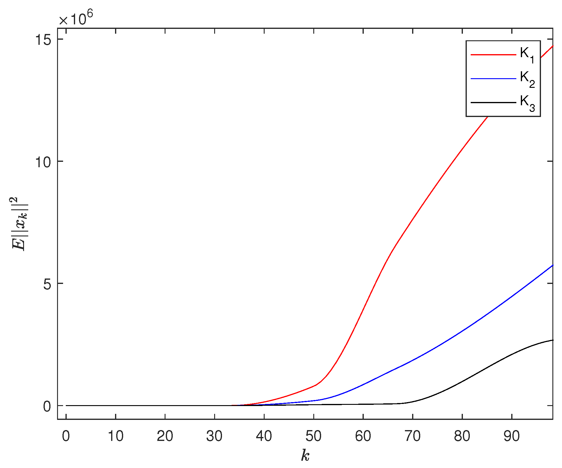
Example 2.
For system , we take the following matrix coefficients into account
In this case, one obtains that the control law follows
To begin with, we first check the given system is not stabilizable in the mean square sense by utilizing inequality (39). Then, to study the essential destabilization, we choose different feedback gain as shown in Table 4. It follows from Theorem 3, the following inequality holds for each , which can be solved by LMI in Matlab with
7. Conclusions
We study the stochastic stabilization problems with the co-existence of input delay and multiplicative noise in the control variable. First, as the necessary condition of asymptotic mean square stabilization, we derive an iterative algorithm to solve the DARE. Then, the concepts of critical stabilization and essential destabilization are defined by operator spectrum theory. Utilizing DLE, the necessary and sufficient conditions are developed for dynamic models under consideration. However, how to utilize the spectrum theory and Lyapunov technology to study the stochastic stabilization for a more general time-delay stochastic system with multiplicative noises remains an open question, which defines a meaningful research direction. On the other hand, applying online Reinforcement Learning (RL) technology to solve DARE with partial system information is another promising research direction.
Author Contributions
Conceptualization, C.T.; methodology, C.T.; software, B.Z.; validation, C.T. and Z.C.; formal analysis, J.D. and M.X.; investigation, J.D. and M.X.; writing—original draft preparation, J.D. and M.X.; writing—review and editing, C.T.; supervision, C.T.; project administration, C.T.; funding acquisition, C.T. and Z.C. All authors have read and agreed to the published version of the manuscript.
Funding
This research was funded by the National Natural Science Foundation of China grant number 62173206; the Natural Science Foundation of Shandong Province grant number ZR2019QF005, ZR2021QF075, ZR2021ZD13; China Postdoctoral Science Foundation grant number 2021M691849.
Institutional Review Board Statement
Not applicable.
Informed Consent Statement
Not applicable.
Data Availability Statement
Not applicable.
Acknowledgments
We would like to thank anonymous reviewers for constructive suggestions to improve the quality of this paper.
Conflicts of Interest
The authors declare no conflict of interest.
References
- Liu, L.; Xie, X. State feedback stabilization for stochastic feedforward nonlinear systems with time-varying delay. Automatica 2013, 49, 936–942. [Google Scholar] [CrossRef]
- Zhang, H.; Li, L.; Xu, J.; Fu, M.Y. Linear quadratic regulation and stabilization of discrete-time systems with delay and multiplicative noise. IEEE Trans. Autom. Control 2015, 60, 2599–2613. [Google Scholar] [CrossRef]
- Mesbah, A. Stochastic model predictive control: An overview and perspectives for future research. IEEE Control Syst. Mag. 2016, 36, 30–44. [Google Scholar]
- Jiang, X.; Zhao, D. Event-triggered fault detection for nonlinear discrete-time switched stochastic systems: A convex function method. Sci. China Inform. Sci. 2021, 64, 200204. [Google Scholar] [CrossRef]
- Zhang, T.; Deng, F.; Sun, Y.; Shi, P. Fault estimation and fault-tolerant control for linear discrete time-varying stochastic systems. Sci. China Inform. Sci. 2021, 64, 200201. [Google Scholar] [CrossRef]
- Wang, Z.; Ho, D.W.C.; Liu, Y.; Liu, X. Robust H∞ control for a class of nonlinear discrete time-delay stochastic systems with missing measurements. Automatica 2009, 45, 684–691. [Google Scholar] [CrossRef] [Green Version]
- Li, X.; Guay, M.; Huang, B.; Fisher, D.G. Delay-Dependent Robust H∞ Control of Uncertain Linear Systems with Input Delay. In Proceedings of the American Control Conference, San Diego, CA, USA, 2–4 June 1999. [Google Scholar]
- Zhao, C.-R.; Zhang, K.; Xie, X.-J. Output feedback stabilization of stochastic feedforward nonlinear systems with input and state delay. Int. J. Robust Nonlinear Control 2016, 26, 1422–1436. [Google Scholar] [CrossRef]
- Krstic, M. Delay Compensation for Nonlinear, Adaptive, and PDE Systems; Birkhäuser Boston: Boston, MA, USA, 2009. [Google Scholar]
- Cacace, F.; Germani, A.; Manes, C. Exponential stabilization of linear systems with time-varying delayed state feedback via partial spectrum assignment. Syst. Control Lett. 2014, 69, 47–52. [Google Scholar] [CrossRef]
- Hou, T.; Zhang, W.; Ma, H. Conditions for essential instability and essential destabilization of linear stochastic systems. In Proceedings of the World Congress on Intelligent Control and Automation, Jinan, China, 7–9 July 2010; pp. 1770–1775. [Google Scholar]
- Hou, T.; Ma, H. A small gain theorem for discrete-time stochastic periodic systems. In Proceedings of the IEEE International Conference on Control and Automation, Kathmandu, Nepal, 1–3 June 2016; pp. 282–287. [Google Scholar]
- Hou, T.; Zhang, W.; Chen, B.S. Regional stability and stabilizability of linear stochastic systems: Discrete-time case. In Proceedings of the IEEE International Conference on Control and Automation, Xiamen, China, 9–11 June 2010; pp. 1660–1665. [Google Scholar]
- Peaucelle, D.; Arzelier, D.; Bachelier, O.; Bernussou, J. A new robust D-stability condition for real convex polytopic uncertainty. Syst. Control Lett. 2000, 40, 21–30. [Google Scholar] [CrossRef]
- Dragan, V.; Morozan, T. Observability and detectability of a class of discrete-time stochastic linear systems. IMA J. Math. Control Inform. 2006, 23, 371–394. [Google Scholar] [CrossRef]
- Tan, C.; Zhang, H.; Wong, W.S. Delay-dependent algebraic Riccati equation to stabilization of networked control systems: Continuous-time case. IEEE Trans. Cybern. 2018, 48, 2783–2794. [Google Scholar] [CrossRef] [PubMed]
- Tan, C.; Zhang, H. Necessary and sufficient stabilizing conditions for networked control systems with simultaneous transmission delay and packet dropout. IEEE Trans. Autom. Control 2017, 62, 4011–4016. [Google Scholar] [CrossRef]
- Zhang, H.; Xie, L. Linear quadratic regulation for discrete-time systems with multiplicative noises and input delays. In Proceedings of the American Control Conference, Minneapolis, MN, USA, 14–16 June 2006; pp. 1718–1723. [Google Scholar]
- Sipahi, R.; Niculescu, S.-I.; Abdallah, C.T.; Michiels, W.; Gu, K. Stability and Stabilization of Systems with Time Delay. IEEE Control Syst. Mag. 2011, 31, 38–65. [Google Scholar]
- Zhang, W.; Zhang, H.; Chen, B.S. Generalized Lyapunov Equation Approach to State-Dependent Stochastic Stabilization/Detectability Criterion. IEEE Trans. Autom. Control 2008, 53, 1630–1642. [Google Scholar] [CrossRef]
- Hou, T.; Zhang, W.; Ma, H. Essential instability and essential destabilisation of linear stochastic systems. IET Control Theory Appl. 2011, 5, 334–340. [Google Scholar] [CrossRef]
- Freiling, G.; Jank, G.; Abou-Kandil, H. Generalized Riccati difference and differential equations. Linear Algebra Its Appl. 1996, 241, 291–303. [Google Scholar] [CrossRef] [Green Version]
- Ran, A.C.M.; Vreugdenhil, R. Existence and comparison theorems for algebraic Riccati equations for continuous- and discrete-time systems. Linear Algebra Its Appl. 1988, 99, 63–83. [Google Scholar] [CrossRef] [Green Version]
- Huang, Y.; Zhang, W.; Zhang, H. Infinite horizon linear quadratic optimal control for discrete-time stochastic systems. Asian J. Control 2008, 10, 608–615. [Google Scholar] [CrossRef]
- Zhang, W.; Chen, B.S. On stabilizability and exact observability of stochastic systems with their applications. Automatica 2004, 40, 87–94. [Google Scholar] [CrossRef]
- Rami, M.A.; Zhou, X.Y. Linear Matrix Inequalities, Riccati Equations, and Indefinite Stochastic Linear Quadratic Controls. IEEE Trans. Autom. Control 2000, 45, 1131–1143. [Google Scholar] [CrossRef]
- Feng, Y.; Anderson, B.D.O. An iterative algorithm to solve state-perturbed stochastic algebraic Riccati equations in LQ zero-sum games. Syst. Control Lett. 2010, 59, 50–56. [Google Scholar] [CrossRef]
- Rami, M.A.; Chen, X.; Moore, J.B.; Zhou, X.Y. Solvability and asymptotic behavior of generalized Riccati equations arising in indefinite stochastic LQ controls. IEEE Trans. Autom. Control 2002, 46, 428–440. [Google Scholar] [CrossRef] [Green Version]
- Tan, C.; Yang, L.; Zhang, F.; Zhang, Z.; Wong, W.S. Stabilization of discrete time stochastic system with input delay and control dependent noise. Syst. Control Lett. 2019, 123, 62–68. [Google Scholar] [CrossRef]
- Tan, C.; Wong, W.S.; Zhang, H. On delay-dependent algebraic Riccati equation. IET Control Theory Appl. 2017, 11, 2506–2513. [Google Scholar] [CrossRef]
- Hou, T.; Zhang, W.; Chen, B.S. Study on general stability and stabilizability of linear discrete-time stochastic systems. Asian J. Control 2011, 13, 977–987. [Google Scholar] [CrossRef]
Figure 1.
Simulation of with .


Table 1.
Three sets of values of real system parameters in stochastic system .
| A | B | C | |
|---|---|---|---|
| 1 | |||
| 2 | |||
| 3 |
Table 2.
Three sets of simulation results of LMI toolbox.
| H | Z | ||
|---|---|---|---|
| 1 | |||
| 2 | |||
| 3 |
Table 3.
Results of three sets of simulation series.
| N | ||
|---|---|---|
| 1 | > 0 | 11 |
| 2 | > 0 | 27 |
| 3 | > 0 | 19 |
Table 4.
Results of three kinds of feedback design for the system.
| K | ||||
|---|---|---|---|---|
| 1 | ||||
| 2 | ||||
| 3 |
Publisher’s Note: MDPI stays neutral with regard to jurisdictional claims in published maps and institutional affiliations. |
© 2022 by the authors. Licensee MDPI, Basel, Switzerland. This article is an open access article distributed under the terms and conditions of the Creative Commons Attribution (CC BY) license (https://creativecommons.org/licenses/by/4.0/).
Share and Cite
MDPI and ACS Style
Tan, C.; Di, J.; Xiang, M.; Chen, Z.; Zhu, B. Stochastic Stabilization for Discrete-Time System with Input Delay and Multiplicative Noise in Control Variable. Processes 2022, 10, 989. https://0-doi-org.brum.beds.ac.uk/10.3390/pr10050989
AMA Style
Tan C, Di J, Xiang M, Chen Z, Zhu B. Stochastic Stabilization for Discrete-Time System with Input Delay and Multiplicative Noise in Control Variable. Processes. 2022; 10(5):989. https://0-doi-org.brum.beds.ac.uk/10.3390/pr10050989
Chicago/Turabian StyleTan, Cheng, Jianying Di, Mingyue Xiang, Ziran Chen, and Binlian Zhu. 2022. "Stochastic Stabilization for Discrete-Time System with Input Delay and Multiplicative Noise in Control Variable" Processes 10, no. 5: 989. https://0-doi-org.brum.beds.ac.uk/10.3390/pr10050989
Note that from the first issue of 2016, this journal uses article numbers instead of page numbers. See further details here.