Early Afterdepolarisations Induced by an Enhancement in the Calcium Current

Abstract

Excitable biological cells, such as cardiac muscle cells, can exhibit complex patterns of oscillations such as spiking and bursting. Moreover, it is well known that an enhancement in calcium currents may yield certain kind of cardiac arrhythmia, so-called early afterdepolarisations (EADs). The presence of EADs strongly correlates with the onset of dangerous cardiac arrhythmia. In this paper we study mathematically and numerically the dynamics of a cardiac muscle cell with respect to the calcium current by investigating a simplistic system of differential equations. For the study of this phenomena, we use bifurcation theory, numerical bifurcation analysis, geometric singular perturbation theory and computational methods to investigate a nonlinear multiple time scales system. It will turn out that EADs related to an enhanced calcium current are canard–induced and that we have to combine these theories to derive a better understanding of the dynamics behind EADs. Moreover, a suitable time scale separation argument determines the important and sensitive system parameters which are related to the occurrence of EADs.

1. Introduction

The aim of this manuscript is the mathematical and numerical investigation of a four dimensional version of the model introduced in [1] with respect to an enhancement in the calcium current, which is already used to study early afterdepolarisations (EADs)—a special type of cardiac arrhythmia—induced by a reduced potassium current. We will show reasons for the occurrence of EADs via an enhancement in the calcium current, using numerical bifurcation analysis and geometric singular perturbation theory (GSPT). One main advantage of the GSPT, which is an analytic technique for multi-scale problems that combines asymptotic theory with dynamical techniques, is the study of a reduced model, i.e., a subsystem. This approach is very useful and shows some mechanisms yielding EADs. Moreover, this ansatz is very valuable to identify the sensitive parameters of the system. Nevertheless, it turns out that not all details can be explained using GSPT. Thus, a combination of both theories—bifurcation theory and geometric singular perturbation theory—is needed. We will explain our approach for this simplified model, but of course we can use this ansatz also for more complex models, cf. [2,3].

In general, EADs are additional small amplitude spikes during the plateau or the repolarisation phase of the action potential (AP), i.e., pathological voltage oscillations during one of these phases. They are caused by ion channel diseases, oxidative stress or drugs and are often associated with deficiencies in potassium currents or enhancements in calcium currents [4]. Furthermore, the presence of EADs strongly correlates with the onset of dangerous cardiac arrhythmias, including torsades de pointes (TdP), which is a specific type of abnormal heart rhythm that can lead to sudden cardiac death, see [5,6,7,8,9,10]. Furthermore, EADs are so-called mixed-mode oscillations (MMOs) [11], i.e., complex oscillatory waveforms that naturally occur in physiologically relevant dynamical processes. MMOs correspond to the switching between small amplitude oscillations and relaxation oscillations.

In this paper, we will use the geometric singular perturbation theory [11,12] and bifurcation analysis [13] to investigate reasons for the appearing of EADs. Here, we are focused on EADs related to an enhancement in the calcium currents, see [14,15]. The main novelty is the combination of these theories to study EADs and mainly the use of the needed time scale separation argument to derive the parameter sensitivity of the considered system. Moreover, we will show that the mathematical approach which is used for instance in [1] is limited to the study of EADs related to an inhibited potassium current. We will see that the considered system exhibits up to four different time scales depending on the different system parameters.

The paper is organised as follows. We start with a brief introduction into the topic of cardiac APs and arrhythmia, i.e., afterdepolarisations, see Section 1.1. Then, in Section 1.2 we will go on with the mathematical modelling of cardiac APs using a Hodgkin-Huxley type formalism. For our mathematical and numerical analysis of the dynamics of our model, we will use the GSPT and bifurcation analysis. Therefore, in Section 2.1 we will give a brief introduction into the topic of GSPT. This theory we will utilise in Section 2.2 and it turns out that EADs related to an enhanced calcium current are canard–induced MMOs. Nevertheless, in Section 2.3 we will show that the study of the reduced system does not show all details of the occurrence of EADs. Therefore, we are also using numerical bifurcation analysis. The desired bifurcation diagram we will derive utilising the MATLAB toolboxes MATCONT and CL_MATCONT [16,17,18], which are numerical continuation packages for the interactive bifurcation analysis of dynamical systems. Finally, in Section 3 we will discuss our results.

1.1. Biological and Mathematical Background

An AP is a temporary, characteristic variance in the membrane potential of an excitable biological cell, e.g., neuron or cardiac muscle cell, from its resting potential. The molecular mechanism of an AP is based on the interaction of voltage-sensitive ion channels. The reason for the formation and the special properties of the AP is established in the properties of different groups of ion channels in the plasma membrane. An initial stimulus activates the ion channels as soon as a certain threshold potential is reached. Then, these ion channels break open and/or up such that this interaction allows an ion current flow, which changes the membrane potential. A normal AP is always uniform and the cardiac muscle cell AP is typically divided into four phases, i.e., the resting phase, the upstroke phase, the (long) plateau phase and the repolarisation phase, see for more details [15]. The resting phase is designated by high potassium ($K^{+}$) currents. After the initial stimulus the sodium ($N{a}^{+}$) conductance increases rapidly and the $N{a}^{+}$ current flux into the cardiac muscle cell until a spike potential is achieved. Then, the $N{a}^{+}$ current inactivates rapidly followed by the activation of L-type calcium ($C{a}^{2+}$) current. The $C{a}^{2+}$ current is more slowly than the $N{a}^{+}$ current and plays a key role in maintaining the long plateau phase, which is characteristic for the cardiac muscle cell. While the $C{a}^{2+}$ conductance increases the $K^{+}$ conductance decreases. The plateau phase is followed by a repolarisation phase, where the intrinsic $K^{+}$ ion channels are activated and this is connected with the reduction of the $C{a}^{2+}$ conductance. Finally, the $K^{+}$ current increases until the resting phase is reached. If there are depolarising variations of the membrane voltage, then we are speaking about afterdepolarisations. These afterdepolarisations are divided into EADs and delayed afterdepolarisations (DADs). This division depends on the timing obtaining of the AP. EADs occur either in the plateau or in the repolarisation phase of the AP and are benefited by an elongation of the AP, while DADs occur after the repolarisation phase is completed. EADs are resulting for example from a reduction of the repolarising $K^{+}$ currents. Triggers for this are congenital disorders of the ion channels or the ingestion of some medicament. The elongation of the AP can generate afterpolarisations by reactivation L-type $C{a}^{2+}$ influx. Also chronic cardiac insufficiency may appear with an elongation of the AP by a reduction of the repolarising $K^{+}$ currents.

1.2. The Mathematical Model

The history of the modelling of APs of excitable biological cells as neurons and cardiac muscle cells starts with the famous and pioneering Hodgkin-Huxley model in 1952 [19]. In this paper, the authors established a mathematical approach that can be used to model an AP of excitable biological cells, i.e., one uses a Hodgkin-Huxley (type) formalism for the description of APs as systems of ordinary differential equations. The first model of a cardiac cell is the Noble model [20] of a generic Purkinje cell. In 1991, Luo and Rudy published an ionic model for cardiac action potential in guinea pig ventricular cells. Moreover, the Ten Tusscher-Noble-Noble-Panfilov model [21] from 2004 describes a model for human ventricular tissue, cf. also [2]. Such conductance-based models are based on an equivalent circuit representation of a cell membrane. These models represent a minimal biophysical interpretation for an excitable biological cell in which current flow across the membrane is due to charging of the membrane capacitance and movement of ions across ion channels. Ion channels are selective for particular ionic species, such as calcium ($C{a}^{2+}$) or potassium ($K^{+}$), giving rise to currents $I_{C{a}^{2+}}$ or $I_{K^{+}}$, respectively. Our simplistic model reads as follows:

$$\frac{\mathrm{d}V}{\mathrm{d}t}=-\frac{I_{K^{+}}+I_{C{a}^{2+}}}{C_m},$$

(1)

with the membrane capacity $C_m=1\frac{\mu F}{m^2}$ and ion currents

$$I_{K^{+}}:=G_{K^{+}}·x·(V-E_{K^{+}})\mathrm{and}{I}_{C{a}^{2+}}:=G_{C{a}^{2+}}·d·f·(V-E_{C{a}^{2+}}),$$

(2)

where the different gating variables d, f and x are satisfying the differential equation

$$\frac{\mathrm{d}y}{dt}=\frac{y_{\infty }\left(V\right)-y}{{\tau }_y}$$

(3)

and y represents the gating variables d, f and x, while

$$\begin{array}{c}\hfill y_{\infty }:=y_{\infty }\left(V\right)=\frac{1}{1+exp\left(\frac{V-V_{T_y}}{k_y}\right)}\end{array}$$

(4)

with $V_{T_y}\in \mathbb{R}$, $k_y\in \mathbb{R}\backslash \left\{0\right\}$ denotes the equilibrium of the corresponding gating variable and ${\tau }_y$ is the corresponding relaxation time constant for each of d, f and x. The gating variables d, f and $x\in [0,1]$ are important for the activation (opening) and inactivation (closing) of the ion channels and therefore for the ion current interaction, see [15]. Moreover, the Nernst potentials of these ion currents are denoted by $E_{C{a}^{2+}}$ and $E_{K^{+}}$, while the corresponding conductance are represented by $G_{C{a}^{2+}}=0.025\frac{mS}{c{m}^2}$ and $G_{K^{+}}=0.05\frac{mS}{c{m}^2}$, respectively. Furthermore, the relaxation time constants are given by ${\tau }_f=80$ ms and ${\tau }_x=300$ ms. We have to remark that in [1] it is assumed that the gating variable d is equal to its steady state. Please note that if ${\tau }_d$ tends to zero, we have the situation as in [1], since

$${\tau }_d\frac{\mathrm{d}d}{dt}=(d_{\infty }-d)\Rightarrow 0=(d_{\infty }-d),$$

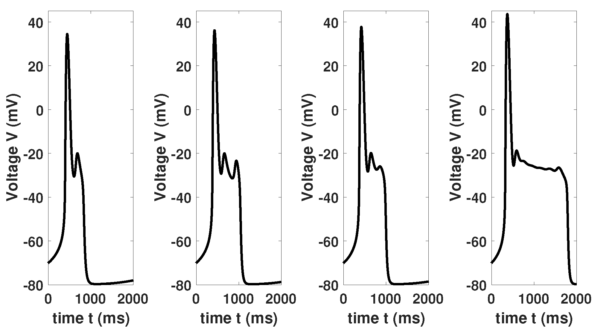
as ${\tau }_d\to 0$. In this paper, we will use the relaxation time constant of d, i.e., ${\tau }_d$, as further non-zero parameter. Moreover, the choice ${\tau }_d=0.1$ ms yields the same trajectory as in [1], but also smaller values of ${\tau }_d$ are conceivable. In Figure 1 some examples of EADs are presented with ${\tau }_d=0.1$ ms and $G_{C{a}^{2+}}\in \left\{0.029\frac{mS}{c{m}^2};0.03\frac{mS}{c{m}^2};0.031\frac{mS}{c{m}^2};0.035\frac{mS}{c{m}^2}\right\}$ (from left to right). Please compare Figure 6a in [15] with the second trajectory in Figure 1. Here, we see that the four dimensional system behaves very similar to the three dimensional system, provided ${\tau }_d$ is small enough and the other system parameters are the same. Moreover, we want to highlight that in [1] the authors basically studied the influence of ${\tau }_x\to \infty$, while in [15] the influence of mainly $G_{C{a}^{2+}}$ and $G_{K^{+}}$ is investigated. In this paper, we are focused on the influence of more system parameter and the identification of their importance. Therefore, we will consider in the following ${\tau }_d=20$ ms. This will help to understand the complex dynamics of the considered system.

2. Investigation of EADs Using GSPT and Bifurcation Analysis

In this section, will study and analyse system (1). To this aim we will use the geometric singular perturbation theory, numerical bifurcation analysis and computational mathematics.

2.1. Brief Introduction into the GSPT

Here, we give a brief overview on the topic of GSPT. In general, a slow-fast system is of the form

$$\begin{array}{c}\hfill \left\{\begin{array}{cc}{\displaystyle \epsilon \frac{\mathrm{d}x}{\mathrm{d}\tau }}\hfill & =F(x,y,p,\epsilon ),\hfill \\ \hfill {\displaystyle \frac{\mathrm{d}y}{\mathrm{d}\tau }}& =G(x,y,p,\epsilon ),\hfill \end{array}\right.\end{array}$$

(5)

where $0\le \epsilon \ll 1$, $x\in {\mathbb{R}}^m$, $y\in {\mathbb{R}}^n$, $p\in {\mathbb{R}}^r$ with $m,n\ge 1$ and $r\ge 0$. We denote by x and y the state space variables and by p the system parameters, while the small parameter $\epsilon$ represents the ratio of time scales. Moreover, the functions $F:{\mathbb{R}}^m\times {\mathbb{R}}^n\times {\mathbb{R}}^r\times \mathbb{R}\to {\mathbb{R}}^m$ and $G:{\mathbb{R}}^m\times {\mathbb{R}}^n\times {\mathbb{R}}^r\times \mathbb{R}\to {\mathbb{R}}^n$ are assumed to be sufficiently smooth, typically $C^{\infty }$. The space variables x are called fast variables, while the space variables y are called slow variables. Moreover, $\tau$ denotes the slow time scale and the fast time scale t is given by $t=\tau /\epsilon$. If we rescale the system (5) in time—switching from the slow time scale to the fast one—we arrive at

$$\begin{array}{c}\hfill \left\{\begin{array}{cc}{\displaystyle \frac{\mathrm{d}x}{\mathrm{d}t}}\hfill & =F(x,y,p,\epsilon ),\hfill \\ \hfill {\displaystyle \frac{\mathrm{d}y}{\mathrm{d}t}}& =\epsilon G(x,y,p,\epsilon ).\hfill \end{array}\right.\end{array}$$

(6)

In general, solutions of slow-fast systems frequently exhibit slow and fast epochs characterised by the speed at which the solution advances. If $\epsilon$ tends to zero, the trajectories of (5) converge during the slow epochs to the solution of the slow flow/slow subsystem or reduced system

$$\begin{array}{c}\hfill \left\{\begin{array}{cc}\hfill 0& =F(x,y,p,0),\hfill \\ {\displaystyle \frac{\mathrm{d}y}{\mathrm{d}\tau }}\hfill & =G(x,y,p,0),\hfill \end{array}\right.\end{array}$$

(7)

while during fast epochs the trajectories of (6) converge to the fast subsystem or layer problem

$$\begin{array}{c}\hfill \left\{\begin{array}{cc}{\displaystyle \frac{\mathrm{d}x}{\mathrm{d}t}}\hfill & =F(x,y,p,0),\hfill \\ \hfill {\displaystyle \frac{\mathrm{d}y}{\mathrm{d}t}}& =0.\hfill \end{array}\right.\end{array}$$

(8)

The fast subsystem describes the evolution of the fast variables $x\in {\mathbb{R}}^m$ for fixed $y\in {\mathbb{R}}^n$, while the slow subsystem describes the evolution of the slow variables $y\in {\mathbb{R}}^n$. The phase space of the slow flow (reduced problem) is the critical manifold $C_0$, which is defined by $C_0:=\left\{(x,y)\in {\mathbb{R}}^m\times {\mathbb{R}}^n:F(x,y,p,0)=0\right\}.$ A subset $S\subset C_0$ is called normally hyperbolic if the $m\times m$ matrix $\left(D_{x}F\right)$ of the first partial derivatives with respect to the fast variables x, i.e., the Jacobian of F with respect to x, has no eigenvalues with zero real part for all $(x,y)\in S$. Moreover, we call a normally hyperbolic subset $S^a\subset C_0$ attracting if all eigenvalues of $\left(D_{x}F\right)$ have negative real parts, while we call a normally hyperbolic subset $S^r\subset C_0$ repelling if all eigenvalues of $\left(D_{x}F\right)$ have positive real parts. If $S\subset C_0$ is normally hyperbolic and neither attracting nor repelling, it is of saddle type. Usually, the interesting dynamics are localised around these non-hyperbolic regions. There may be isolated points in $C_0$, i.e., folded singularities, satisfying $\left(D_{y}F\right)G(x,y,p,0)=\mathbf{0}\in {\mathbb{R}}^m$ and $\mathrm{rk}\left(D_{x}F\right)(x,y,p,0)=m-1$, where the trajectories of the slow flow switch from incoming to outgoing. Away from fold points the implicit function theorem implies that $C_0$ is locally the graph of a function $h\left(y\right)=x$. Then, the reduced system (7) can be expressed as $\dot{y}=G(h\left(y\right),y,p,0)$, where $\dot{y}=\mathrm{d}y/\mathrm{d}\tau$. However, it is more convenient to write the slow flow in terms of the fast variables x and we can keep the differential-algebraic equations structure of (7). To this aim we determine the total (time) derivative of $F(x,y,p,0)=0$. This yields $\left(D_{x}F\right)\dot{x}+\left(D_{y}F\right)\dot{y}=0$ and we can write the slow flow (7) as the restriction to $C_0$ of the vector field

$$\begin{array}{c}\hfill \left\{\begin{array}{cc}\dot{x}\hfill & =-{\left(D_{x}F\right)}^{-1}\left(D_{y}F\right)G(x,y,p,0),\hfill \\ \dot{y}\hfill & =G(x,y,p,0).\hfill \end{array}\right.\end{array}$$

(9)

This vector field blows up if F is singular and the slow flow is not defined on $\mathbb{F}$, i.e., the set of folded singularities, before desingularisation. Therefore, we consider the desingularised reduced system, which is given by

$$\begin{array}{c}\hfill \left\{\begin{array}{cc}{\displaystyle \frac{\mathrm{d}x}{\mathrm{d}{\tau }_1}}\hfill & =\left(D_{y}F\right)G(x,y,p,0),\hfill \\ {\displaystyle \frac{\mathrm{d}y}{\mathrm{d}{\tau }_1}}\hfill & =-\left(D_{x}F\right)G(x,y,p,0)\hfill \end{array}\right.\end{array}$$

(10)

restricted to $C_0$, where we rescaled the time by $\tau =-\left(D_{x}F\right)·{\tau }_1$. Moreover, ordinary singularities satisfy $G(x,y,p,0)=\mathbf{0}\in {\mathbb{R}}^n$ are equilibria of the desingularised reduced system (10), the reduced system (9) and can be equilibria of the original system (5). Against it folded singularities are in general no equilibria of the reduced system (9) and of the original system (5). Notice that in the reduced system (9) folded singularities are special points, since both sides of the first equation vanish simultaneously. This means that there is potentially a cancellation of a simple zero, i.e., $\dot{x}$ is finite and non-zero at a folded singularity. This allows trajectories to cross the fold in finite time. Such solutions are called singular canards and their persistence under small perturbations gives rise to complex dynamics. If $n\ge 2$, the Jacobian of (10) evaluated at the folded singularities has $(n-2)$ zero eigenvalues and two remaining eigenvalues ${\lambda }_{1,2}$. Moreover, the folded singularities are classified as follows

$$\begin{array}{c}\hfill \left\{\begin{array}{cc}\mathrm{folded}\mathrm{saddle},\hfill & \mathrm{if}{\lambda }_{1,2}\in \mathbb{R}\mathrm{and}{\lambda }_1{\lambda }_2<0,\hfill \\ \mathrm{folded}\mathrm{saddle}-\mathrm{node},\hfill & \mathrm{if}{\lambda }_{1,2}\in \mathbb{R}\mathrm{and}{\lambda }_1{\lambda }_2=0,\hfill \\ \mathrm{folded}\mathrm{node},\hfill & \mathrm{if}{\lambda }_{1,2}\in \mathbb{R}\mathrm{and}{\lambda }_1{\lambda }_2>0,\hfill \\ \mathrm{folded}\mathrm{focus},\hfill & \mathrm{if}{\lambda }_{1,2}\in \mathbb{C}.\hfill \end{array}\right.\end{array}$$

(11)

Here, we have to highlight that folded saddles, folded nodes and folded foci are also known as canard points, see [22]. Even more, for sufficiently small values of the perturbation parameter $\epsilon$ it is possible to calculate the maximal number of small oscillations of a MMO pattern, see [23,24]. For instance, if ${\lambda }_1$ and ${\lambda }_2$ are the eigenvalues of the linearisation of the desingularised system at a folded node and $\mu ={\lambda }_1/{\lambda }_2$ with $|{\lambda }_1|<|{\lambda }_2|$, then the maximal number of small oscillations in the MMO (in a neighbourhood of the folded node) is given by

$$\begin{array}{c}\hfill s_{max}:=⌊\frac{\mu +1}{2\mu }⌋,\end{array}$$

(12)

i.e., the greatest integer less than or equal to $(\mu +1)/2\mu$, provided $\sqrt{\epsilon }\ll \mu$.

2.2. The Study of EADs as MMOs

After this short introduction into the topic of GSPT, we will go on with the investigation of the dynamics of our multiple time scale problem. To this aim we first have to derive a suitable model to be able to apply this theory. To determine the different time scales we use a certain type of time scale separation argument, cf. [25]. Thus, we introduce a new (dimensionless) time variable $\tau$ satisfying $t:=k_t·\tau$, where $k_t$ is a reference time. Choosing $k_t={\tau }_f$ and rewriting (1)–(3), we get:

$$\begin{array}{c}\hfill \left\{\begin{array}{cc}\hfill \epsilon ·\dot{V}=& -{\overline{G}}_{K^{+}}x(V-E_{K^{+}})-{\overline{G}}_{{\mathrm{Ca}}^{2+}}d·f(V-E_{{\mathrm{Ca}}^{2+}}):=F_1(V,d,f,x),\hfill \\ \epsilon ·\dot{d}=\hfill & (d_{\infty }-d):=F_2(V,d,f,x)\hfill \\ \hfill \dot{f}=& (f_{\infty }\left(V\right)-f):=G_1(V,d,f,x),\hfill \\ \hfill \dot{x}=& \delta (x_{\infty }\left(V\right)-x):=\delta G_2(V,d,f,x),\hfill \end{array}\right.\end{array}$$

(13)

where we divided the first equation by $G:=max\left\{G_{K^{+}},G_{C{a}^{2+}}\right\}$ and defined ${\overline{G}}_{K^{+}}:=G_{K^{+}}/G$ and ${\overline{G}}_{C{a}^{2+}}:=G_{C{a}^{2+}}/G$ to derive the dimensionless singular perturbation parameters ${\epsilon }_V:=C_m/({\tau }_f·G)$, ${\epsilon }_d:={\tau }_d/{\tau }_f$ and $\delta :={\tau }_f/{\tau }_x$. Using the setting from above we have that $\epsilon \equiv {\epsilon }_d\equiv {\epsilon }_V$ with $0\le \epsilon <\delta \ll 1$, which implies that the system exhibits three different time scales, where d and V are the fastest variables and x the slowest one. First of all, we have to notice that there are several system parameters, which have a huge influence on the time scale separation and the time scales, i.e., ${\tau }_d$, ${\tau }_f$, ${\tau }_x$, $G_{C{a}^{2+}}$, $G_{K^{+}}$ and $C_m$, cf. (13). Our next step is to derive the critical manifold $C_0$. This yields

$$\begin{array}{c}\hfill C_0:=\left\{(V,f):d=d_{\infty }\left(V\right),x=-\frac{{\overline{G}}_{C{a}^{2+}}}{{\overline{G}}_{K^{+}}}·d·f·\frac{(V-E_{C{a}^{2+}})}{(V-E_{K^{+}})}\right\}.\end{array}$$

(14)

We want to highlight that the critical manifold $C_0$ is the same in both cases (V and d are of the same time scale, or V is the fast variable and $d\equiv d_{\infty }$ in the 3D system). Since the critical manifold $C_0$ is the same in both cases and $d=d_{\infty }$ implying that ${\displaystyle \frac{\mathrm{d}{d}_{\infty }}{\mathrm{d}\tau }=\frac{\partial d_{\infty }}{\partial V}\frac{\mathrm{d}V}{\mathrm{d}\tau }}$ one can show that the desingularised slow flow of (13) restricted to $C_0$ is also the same as the one of the three dimensional system with $d\equiv d_{\infty }$. Moreover, for $\epsilon \to 0$ we have the following slow subsystem:

$$\begin{array}{c}\hfill \begin{array}{cc}\hfill 0=& F_1(V,d_{\infty },f,x),\frac{\mathrm{d}f}{\mathrm{d}\tau }=G_1(V,d_{\infty },f,x),\frac{\mathrm{d}x}{\mathrm{d}\tau }=\delta G_1(V,d_{\infty },f,x),\hfill \end{array}\end{array}$$

(15)

and similarly the fast subsystem

$$\begin{array}{c}\hfill \begin{array}{cc}\hfill \frac{\mathrm{d}V}{\mathrm{d}{\tau }_{\mathrm{fast}}}=& F_1(V,d,f,x),\frac{\mathrm{d}d}{\mathrm{d}{\tau }_{\mathrm{fast}}}=F_2(V,d,f,x),\frac{\mathrm{d}f}{\mathrm{d}{\tau }_{\mathrm{fast}}}=0,\frac{\mathrm{d}x}{\mathrm{d}{\tau }_{\mathrm{fast}}}=0.\hfill \end{array}\end{array}$$

(16)

From (10), using ${\displaystyle {\dot{d}}_{\infty }=\frac{\partial d_{\infty }}{\partial V}\dot{V}}$ we can derive immediately the desingularised slow flow:

$$\begin{array}{c}\hfill \left\{\begin{array}{cc}{\displaystyle \frac{\mathrm{d}V}{\mathrm{d}{\tau }_1}}\hfill & =\left({\displaystyle \frac{\partial F_1}{\partial f}}\right)G_1(V,d_{\infty },f,x)+\delta \left({\displaystyle \frac{\partial F_1}{\partial x}}\right)G_2(V,d_{\infty },f,x),\hfill \\ \hfill {\displaystyle \frac{\mathrm{d}f}{\mathrm{d}{\tau }_1}}& {\displaystyle =-\left(\frac{\partial F_1}{\partial V}\right)G_1(V,d_{\infty },f,x),}\hfill \end{array}\right.\end{array}$$

(17)

restricted to $C_0$, where ${\displaystyle \tau =-\left(\frac{\partial F}{\partial V}\right){\tau }_1}$. Remember that system (17) is the desingularised version of

$$\begin{array}{c}\hfill \begin{array}{cc}\hfill {\displaystyle -\left(\frac{\partial F_1}{\partial V}\right)\frac{\mathrm{d}V}{\mathrm{d}{\tau }_1}=}& \left({\displaystyle \frac{\partial F_1}{\partial f}}\right)G_1(V,d_{\infty },f,x)+\delta \left({\displaystyle \frac{\partial F_1}{\partial x}}\right)G_2(V,d_{\infty },f,x),\hfill \\ \hfill \frac{\mathrm{d}f}{\mathrm{d}{\tau }_1}=& G_1(V,d_{\infty },f,x),\hfill \end{array}\end{array}$$

(18)

restricted to $C_0$. An ordinary singularity of (17) is given if $G_1=G_2=0$, while a fold point $z_{•}={(V_{•},d_{\infty }\left(V_{•}\right),f_{•},x_{•})}^T\in \mathbb{F}$ is a folded singularity of (17) if

$$\begin{array}{c}\hfill \frac{\partial F_1}{\partial f}\left(z_{•}\right)·G_1\left(z_{•}\right)+\delta \frac{\partial F_1}{\partial x}\left(z_{•}\right)·G_2\left(z_{•}\right)=0\mathrm{and}\frac{\partial F_1}{\partial V}\left(z_{•}\right)=0.\end{array}$$

This yields explicit expressions for $f_{•}$ and $x_{•}$ depending on $V_{•}$, i.e.,

$$x_{•}=-\frac{{\overline{G}}_{C{a}^{2+}}}{{\overline{G}}_{K^{+}}}{d}_{\infty }\left(V_{•}\right)f_{•}\frac{(V_{•}-E_{C{a}^{2+}})}{(V_{•}-E_{K^{+}})}$$

and

$$f_{•}=\frac{1}{1-\delta }{f}_{\infty }\left(V_{•}\right)+\frac{\delta }{1-\delta }\frac{{\overline{G}}_{K^{+}}(V_{•}-E_{K^{+}})}{{\overline{G}}_{C{a}^{2+}}(V_{•}-E_{C{a}^{2+}})}\frac{x_{\infty }\left(V_{•}\right)}{d_{\infty }\left(V_{•}\right)}.$$

At this stage we see that the shape of the critical manifold is not depending on $\delta$ or the choice of ${\tau }_f$ and ${\tau }_x$, but the location of the folded singularities and their stability. Moreover, notice that the Jacobian of (17) has at least one zero eigenvalue. Furthermore, varying the ratio ${\tau }_f/{\tau }_x$ changes the desingularised slow flow (17). Notice that for $\delta \to 0$ we have an one dimensional slow flow, where f is determined by the critical manifold and x is constant. Therefore, it does not make sense to consider both limits $\epsilon \to 0$ and $\delta \to 0$ simultaneously. However, varying $\delta$ may compensate the effect of an enhanced calcium current, cf. [15]. Moreover, the critical manifold $C_0$ as well as the desingularised slow flow are depending on ${\overline{G}}_{K^{+}}$ and ${\overline{G}}_{C{a}^{2+}}$, cf. (14) and (17). Hence, varying ${\overline{G}}_{K^{+}}$ and/or ${\overline{G}}_{C{a}^{2+}}$ has an influence on (14) and (17). Furthermore, ${\tau }_d$ and $C_m$ have only an influence on the time scale separation argument and after passing to the singular limit $\epsilon \to 0$ our discussion is independent on ${\tau }_d$ and $C_m$.

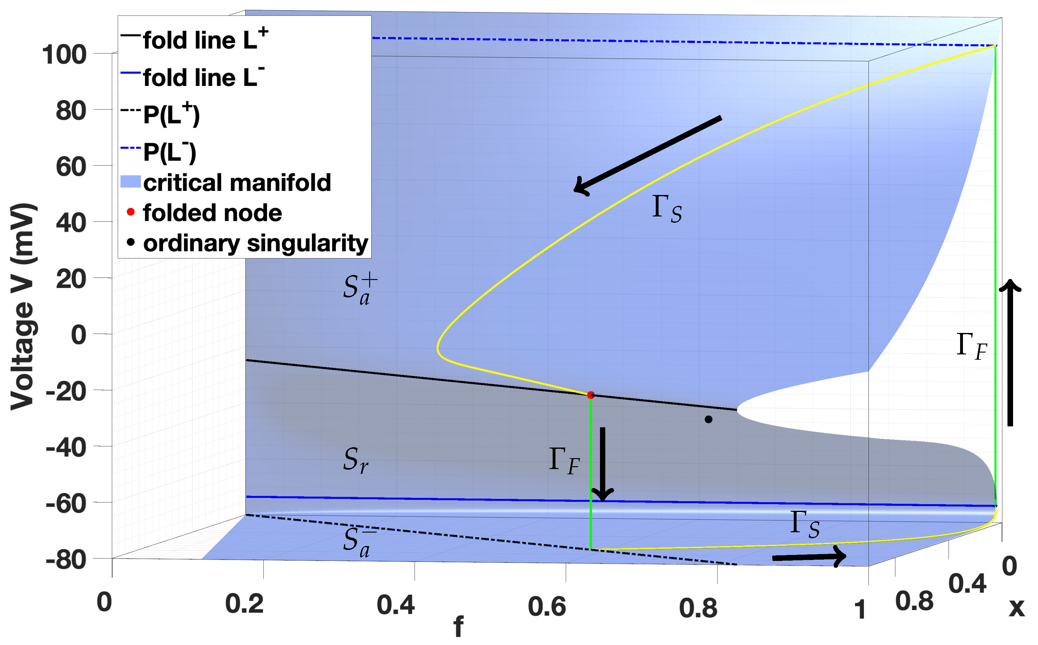
In the following, we consider $G_{C{a}^{2+}}=0.032\frac{mS}{c{m}^2}$. Computing the critical manifold $C_0$ (14) together with two fold lines $L^{\pm }=\left\{(V,d,f,x)\in C_0:{F_1}_V(V,d,f,x)=0,{F_1}_{VV}(V,d,f,x)\ne 0\right\}$, the folded node $(V,f,x)\approx (-24.7923,0.5804,0.7027)$ with eigenvalues ${\lambda }_1\approx -0.1974$ and ${\lambda }_2\approx -1.7305$, an ordinary singularity $(V,f,x)\approx (-30.2250,0.7666,0.8760)$ and the singular orbit, we gain Figure 2. Notice that for ${\tau }_f$ and ${\tau }_x$ satisfying the ratio $\delta ={\tau }_f/{\tau }_x\equiv 4/15$ the folded node will be the same—similarly if $G_{C{a}^{2+}}/G_{K^{+}}=16/25$. The critical manifold is divided into two attracting sheets $S_a^{\pm }$ and one repelling sheet $S^r$, where $S^r$ lies between the two fold lines $L^{\pm }$. The fold lines are nondegenerate since $\partial F_1/\partial f\ne 0$ or $\partial F_1/\partial x\ne 0$ or both is satisfied. Moreover, we have an ordinary singularity on $S^r$. Notice that spiking, bursting and plateauing are only possible provided that the ordinary singularity is unstable, i.e. the ordinary singularity lies on the repelling manifold $S^r$, cf. [26]. The singular or relaxation orbit consists of four distinct segments, i.e., two slow orbit ${\Gamma }_S$ and two fast orbit ${\Gamma }_F$ segments. Notice that in general, singular periodic orbits which are filtered into the folded node on $L^{+}$ are singular representations of MMOs. The aim of GSPT is now to combine information from the reduced and layer problems in order to understand the dynamics of the cell model (1), particularly the oscillatory behaviour. Thus, we use the reduced and the layer flows to construct singular periodic orbits, which—according to GSPT [26,27]—will perturb to nearby periodic orbits of the full system (1) for sufficiently small perturbations.

The singular orbit is constructed as follows. From lower fold line $L^{-}$ there is a rapid evolution ${\Gamma }_F$ described by (16) towards the upper attracting manifold $S_a^{+}$. Once the trajectory reaches $S_a^{+}$ the reduced flow ${\Gamma }_S$ takes over until the trajectory reaches the upper fold line $L^{+}$. Then, at the fold line the reduced flow is singular and there is a finite time blow-up of the solution. The layer problem (16) becomes the appropriate descriptor and there is a fast down-jump to the lower attracting manifold. Here, the reduced system (15) describes the slow motions along the critical manifold until the trajectory once again hits the fold line. The GSPT guarantees that this singular orbit will persist as a nearby periodic relaxation oscillation corresponding to a spiking solution of (1). A folded node occurs in generic slow-fast systems with two (or more) slow variables [22,24,27]. Moreover, a folded node allows for an entire sector of trajectories to pass from the upper attracting branch $S_a^{+}$ of the critical manifold to the repelling branch $S_r$ and to follow that repelling branch for an $\mathcal{O}\left(1\right)$ time on the slow time scale. Notice that solutions of the reduced problem (18) passing through a canard point from an attracting manifold $S_a^{+}$ to a repelling manifold $S_r$ are called singular canards. The sector of canard solutions (the singular funnel, cf. Figure 3) is bounded by the fold line $L^{+}$ and by the strong canard ${\gamma }_S$, which is the unique trajectory tangential to the strong eigendirection of the folded node, cf. [26]. Two singular canards are related to the eigendirections of the folded node, i.e., the weak and strong canards. They correspond to the smallest and largest (in absolute value) eigenvalues respectively.

There are two major requirements that the singularly perturbed system has to satisfy to guarantee the existence of canard-induced MMOs, see [28] and cf. also [23], i.e.,

(a)

The reduced flow (desingularised slow flow) has to possess a folded node.

(b)

There is a singular periodic orbit formed by the slow and fast segments of the reduced and layer problems (slow and fast subsystem) which starts with a fast fiber segment at the folded node. This guarantees that the global return of such singular periodic orbit is within the singular funnel of the folded node.

Both conditions are satisfied in our situation. This implies that the MMOs are canard-induced and we have canard-induced EADs. Moreover, if $\sqrt{\epsilon }\ll \mu ={\lambda }_1/{\lambda }_2\approx 0.1141$, then $s_{max}=4$, cf. (12). Please also note that that system (13) exhibits several types of folded singularities mentioned in (11) for different values of conductance $G_{C{a}^{2+}}$. If we increase $G_{C{a}^{2+}}$ the folded node will travel on the fold line $L^{+}$ to the “right”, which means that the values of f and x at the folded node become bigger. Moreover, the ordinary singularity will travel also towards the folded node until both point collide. Then, the folded node becomes a folded saddle. If the folded node travels to the “left”, then it will become a folded focus for smaller values of $G_{C{a}^{2+}}$. Furthermore, we have a two dimensional fast subsystem, but then this system exhibits only limit point bifurcations and no Andronov-Hopf bifurcations. Hence, there are no Hopf-induced EADs induced by an enhanced calcium current. Thus, we have shown that system (13) exhibits only canard-induced EADs via an enhanced calcium current. Finally, we want to highlight also that system (13) exhibits Hopf-induced EADs provided we consider a fixed singular perturbation parameter $\epsilon$ and $\delta \to 0$. In this case we have a three dimensional fast subsystem with one bifurcation parameter x, but the occurring EADs are then related to a reduced potassium current [1].

2.3. The Study of EADs Using Bifurcation Analysis

In Section 2.2 we established that EADs related to an enhanced calcium current are canard-induced. Here, we did simultaneous the discussion for $G_{C{a}^{2+}}=0.032\frac{mS}{c{m}^2}$ and all $C_m={\tau }_d·G_{K^{+}}$, provided $G_{C{a}^{2+}}\le G_{K^{+}}$. In addition, from (12) we know that $s_{max}=4$ if $\sqrt{\epsilon }\ll 0.1141$. Regarding our setting for the relaxation time constant ${\tau }_d=20$ ms and the membrane capacity $C_m=1\frac{\mu F}{m^2}$ we see that $\sqrt{\epsilon }=0.25\gg 0.1141$ and thus, $s_{max}=4$ is not satisfied. Moreover, for a setting like ${\tau }_d=40$ ms and $C_m=2\frac{\mu F}{m^2}$ one diverges more from the condition $\sqrt{\epsilon }\ll 0.1141$, since $\sqrt{\epsilon }=1/\sqrt{2}$. However, the system still exhibits MMOs or EADs but does not satisfy (12), since the condition $\sqrt{\epsilon }\ll \mu$ is barely to fulfil.

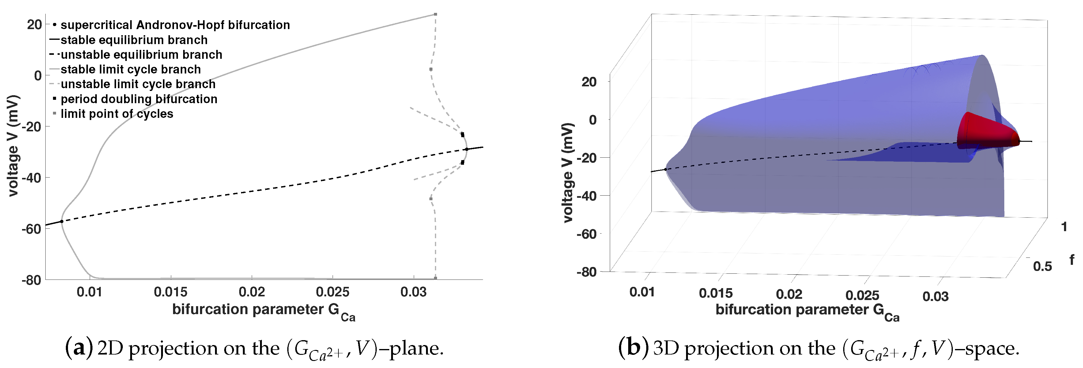
Our next step is the study of system (1) using bifurcation analysis. In general, a bifurcation of a dynamical system is a qualitative change in its dynamics produced by varying parameters. Since we investigate the occurrence of EADs induced by an enhancement in the calcium current $I_{C{a}^{2+}}$, we will choose the conductance $G_{C{a}^{2+}}$ as bifurcation parameter to be able to simulate the decreasing or mainly the increasing of the calcium current. Moreover, we will use our observation from above to analyse the behaviour of system (1). First of all, determining the equilibrium curve of system (1), which is basically the equilibria of this system for different values of $G_{C{a}^{2+}}$, yields two stable branches and one unstable branch for all parameter settings. Depending on the parameter setting the equilibrium curve loses or wins stability via a sub- or supercritical Andronov-Hopf bifurcation, cf. also [15]. An Andronov-Hopf bifurcation is characterised by a pair of purely imaginary eigenvalues, where the equilibrium changes stability and a unique limit cycle bifurcates from it, i.e., it is the birth of a limit cycle. The distinction into sub- or supercritical means that an unstable or stable limit cycle, respectively, bifurcates. For the standard setting ${\tau }_d=20$ ms system (1)–(4) exhibits two supercritical Andronov-Hopf bifurcations (black dots), cf. Figure 4.

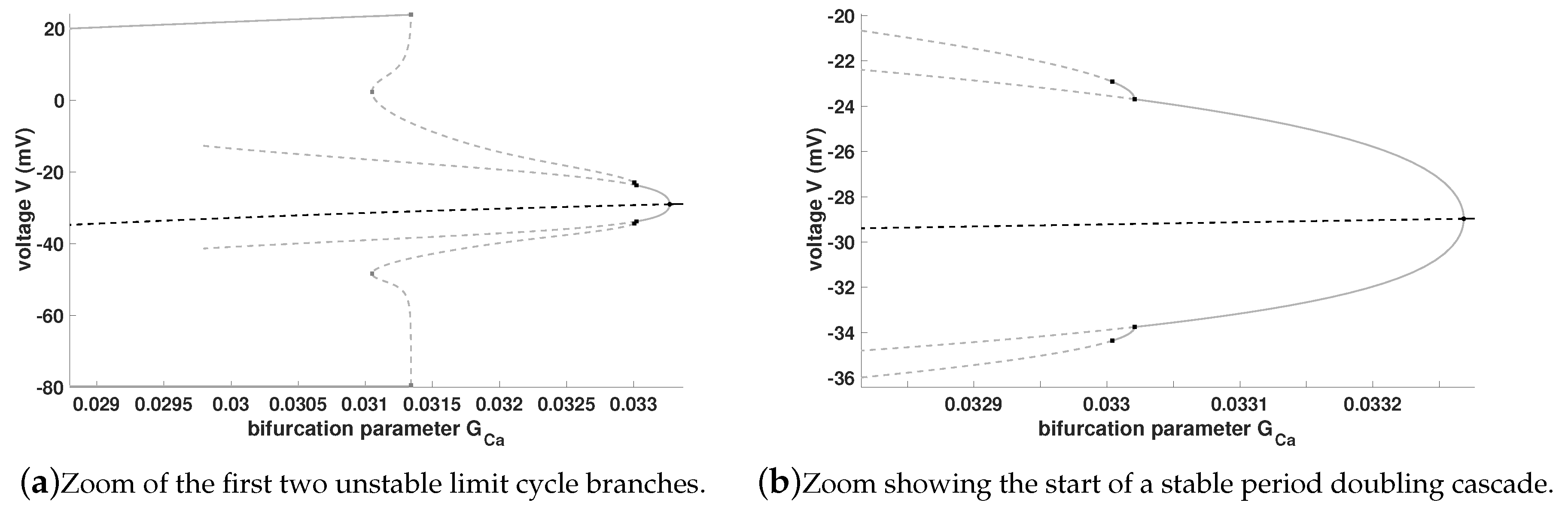
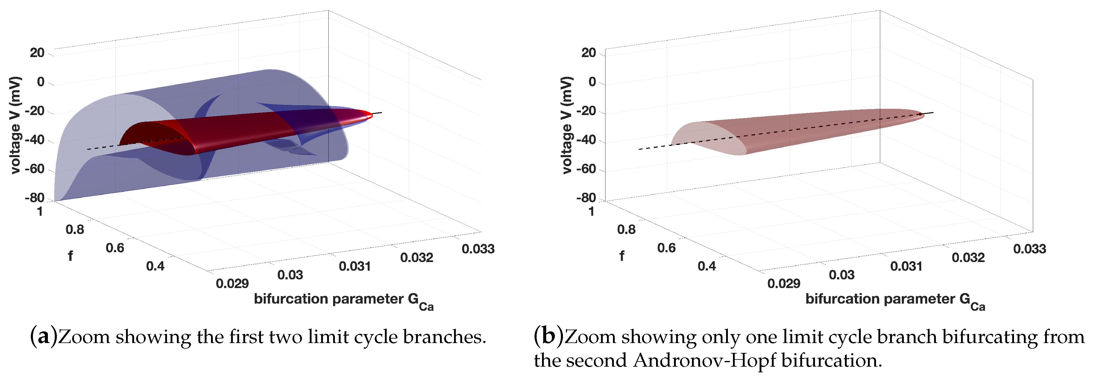
From the first Andronov-Hopf bifurcation ($G_{C{a}^{2+}}\approx 0.008253\frac{mS}{c{m}^2}$) a stable limit cycle branch bifurcates which becomes unstable via a limit point of cycle ($G_{C{a}^{2+}}\approx 0.03134055\frac{mS}{c{m}^2}$) before it wins again stability via a period doubling bifurcation. There is also a second stable limit cycle branch bifurcating from the second Andronov-Hopf bifurcation ($G_{C{a}^{2+}}\approx 0.033268\frac{mS}{c{m}^2}$) which becomes unstable via a period doubling bifurcation (connection of both limit cycle branches), cf. also Figure 5b.

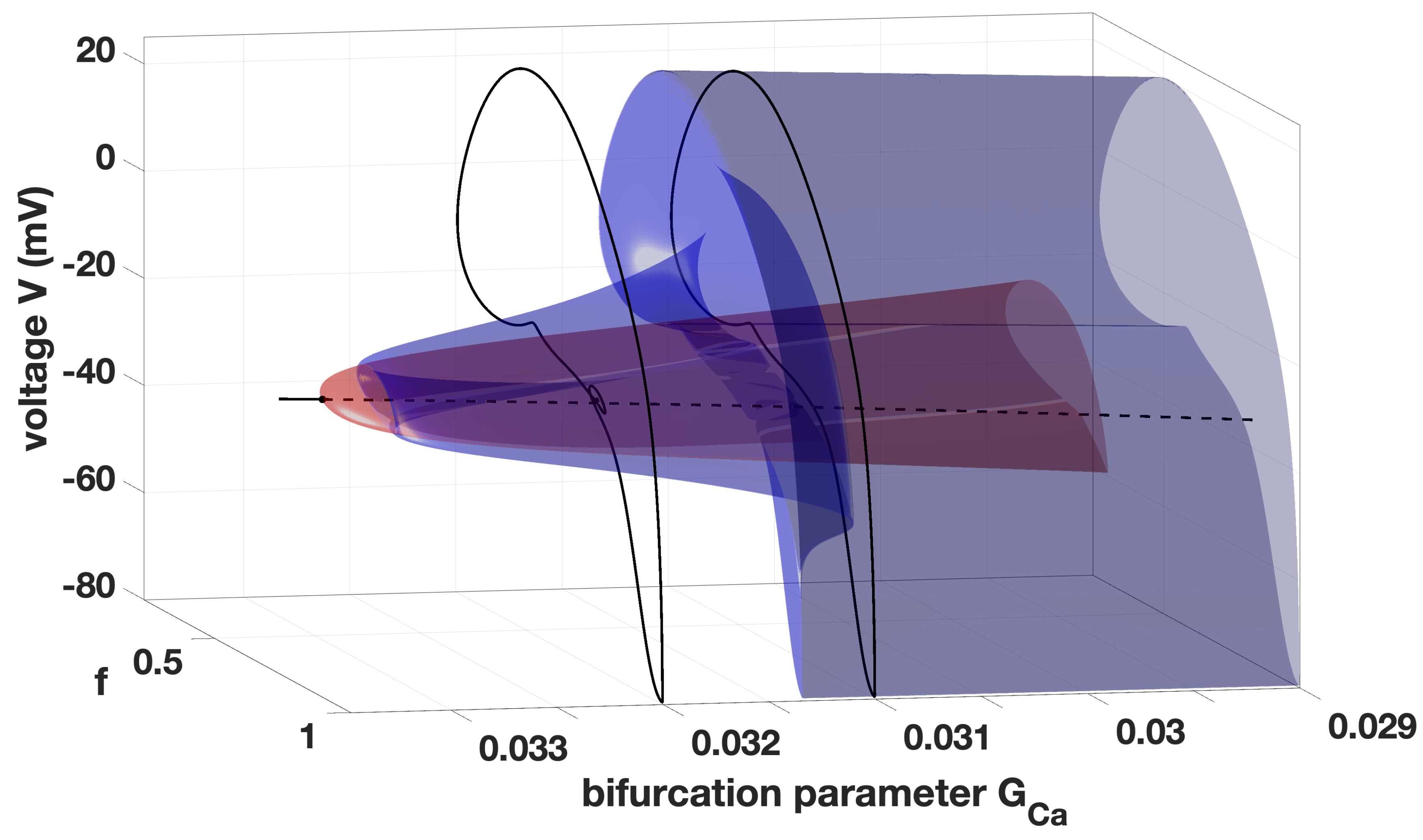
This unstable limit cycle branch has of course influence on the system (1) but it does not yields automatically EADs, it also may correspond to an AP. Notice that the limit cycle branches are determined via a continuation algorithm included in MATCONT. The region between the first Andronov-Hopf bifurcation and the first limit point of cycle ($G_{C{a}^{2+}}\approx 0.03134055\frac{mS}{c{m}^2}$) indicates the region, where no EADs occur, cf. [15]. EADs appear after the first limit point of cycle. In Figure 5a the transient from AP to EADs via the limit point of cycle bifurcation is highlighted, while Figure 5b shows the beginning of a stable period doubling cascade. In Figure 9 we see that this transient might be also via a period doubling bifurcation. Moreover, in Figure 6 we illustrate the limit cycle branches in 3D.

For a better understanding we included in Figure 7 also two trajectories, one represents a normal AP, while the other shows an EAD.

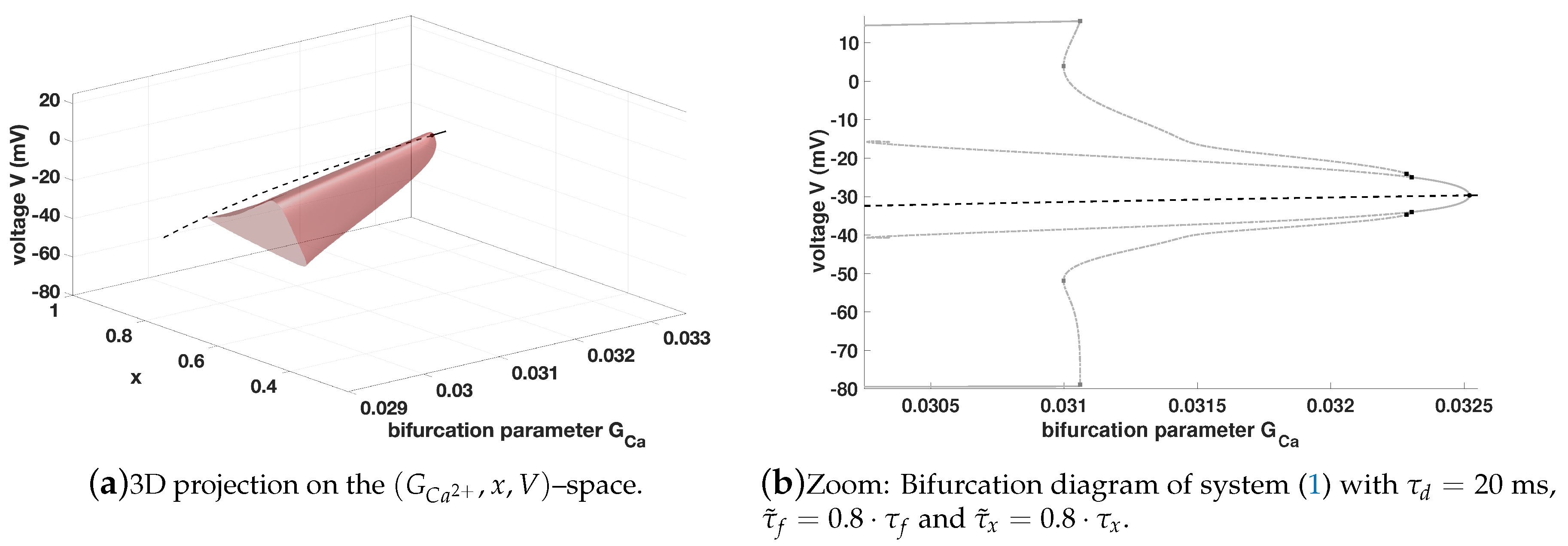
Notice that we have a four dimensional phase space plus a further dimension for the parameter. Therefore, we have a five dimensional object which we can only plot in 2D or 3D as a projection on a 2D plane or 3D space. This makes the visualisation slightly difficult and it becomes more difficult if the dimension of the system increases. Nevertheless, one gets a good description of the behaviour of the considered system using the bifurcation theory. From the 2D and 3D projection in Figure 4, Figure 5 and Figure 6 one might get the impression that the limit cycle starting from the second Andronov-Hopf bifurcation is not completed, but this limit cycle terminates at the unstable equilibrium branch, cf. the projection on the $(G_{C{a}^{2+}},x,V)$–space in Figure 8a. In Figure 8b we show for comparison the corresponding bifurcation diagram with ${\tilde{\tau }}_f=0.8·{\tau }_f$ and ${\tilde{\tau }}_x=0.8·{\tau }_x$ instead of with ${\tau }_f$ and ${\tau }_x$, cf. Figure 5b. Here, one sees that the behaviour is different compared to the standard setting, while in the discussion of the GSPT this change has no influence. Thus, it is important to use both approaches for the investigation of such phenomena.

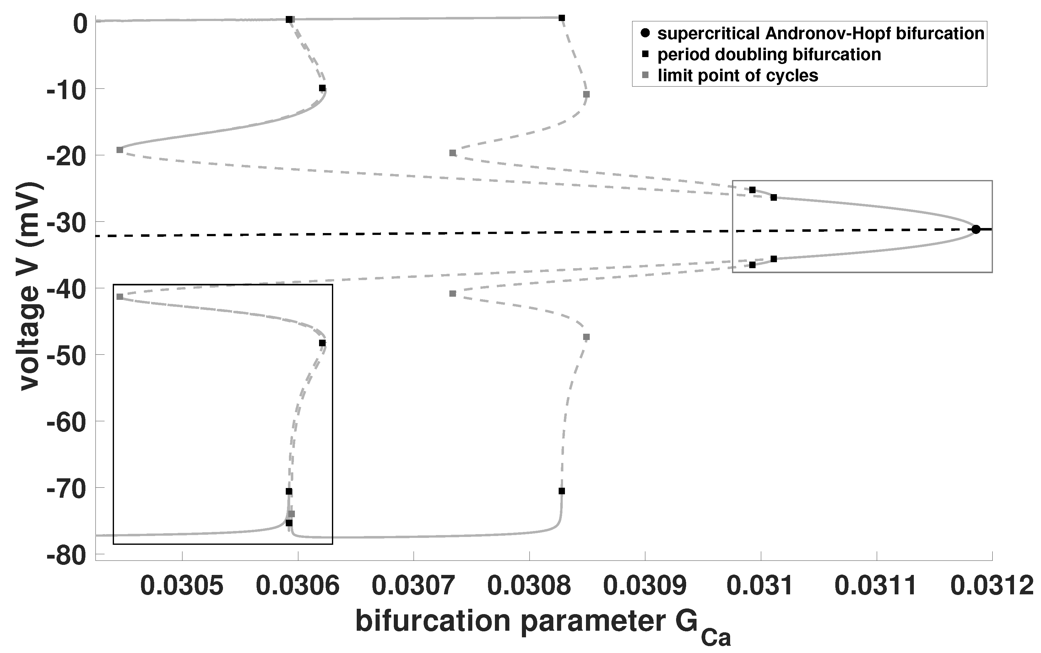
Finally, if we consider the bifurcation diagram of (1)–(3) with ${\tau }_d=40$ ms and $C_m=2\frac{\mu F}{m^2}$ instead of ${\tau }_d=20$ ms and $C_m=1\frac{\mu F}{m^2}$, we see again the importance to consider all these parameters, cf. Figure 9.

In Figure 9 and Figure 10a we see that the system (1) may exhibit different type of MMOs and critical transient regions depending on the choice of the system parameters. Even more, it also shows that $\epsilon =0.5$ in combination with $G_{C{a}^{2+}}=0.032\frac{mS}{c{m}^2}$ does not yield MMOs, cf. Figure 9. The reason for this is that the condition $0<\epsilon \ll 1$ is not suitable satisfied. Notice that there is no explicit condition how small $\epsilon$ has to be, only it has to be much smaller than 1. Nevertheless, Figure 9 shows the system (1) exhibits MMOs, but for smaller values of $G_{C{a}^{2+}}$. For a more suitable visualisation of Figure 9, we present in Figure 10 two zooms of Figure 9. Notice that the system exhibits for this setting two supercritical Andronov-Hopf bifurcations. From the supercritical Andronov-Hopf bifurcation shown in Figure 10b a stable period doubling cascade bifurcates, which is a route to chaos, cf. [29].

Furthermore, we have shown that the GSPT gives information about the nature of the oscillatory behaviour and even more, one can use the GSPT to determine the important system parameters yielding these oscillations. However, we saw that it is not sufficient to consider only one parameter to analyse the complete dynamics of a dynamical system. Here, we have seen the high relevance for the investigation of MMOs in combination with bifurcation analysis to derive a more detailed understanding of EADs, which one can use to prevent them. In [15] some approaches to control the effect of an enhanced calcium current are established and for this aim a further system parameter is highly interesting, e.g., increasing of ${\tau }_d$ may smooth out this effect yielding EADs. Moreover, these observations, i.e., the system exhibits several time scales and MMOs as in Figure 1, motivate the investigation of system (13) in the sense of the geometric singular perturbation theory.

3. Discussion

In this paper we studied the occurrence of EADs in system (1) related to an enhancement in the calcium current. More precisely, we investigated the sensitivity of the system related to parameter changes. To this aim we used bifurcation theory, numerical bifurcation analysis and GSPT. Moreover, because of the fact that EADs may appear via an enhancement in the calcium current we used the conductance of the calcium current as bifurcation parameter to study the behaviour of system (1) under the influence of an enhanced calcium current. Furthermore, a time scale separation argument motivates to consider further important parameters, cf. (13). Under the assumption that stress, drugs or any diseases have no influence on the steady states of the gating variables, i.e., $d_{\infty }$, $f_{\infty }$ and $x_{\infty }$, we discussed the behaviour of (13) with respect to changes in ${\tau }_d$, ${\tau }_f$, ${\tau }_x$, $C_m$, $G_{C{a}^{2+}}$ and $G_{K^{+}}$. Summarising we have shown that system (1) exhibits MMOs or EADs. These MMOs may appear as Hopf-induced MMOs via a reduction of the potassium current or as canard-induced MMOs related to the calcium dynamics of the system. Thus, we pointed out that system (13) may exhibits Hopf-induced EADs only if ${\tau }_x\to \infty$, which may yield plateau or pseudo-plateau bursting, cf. [30,31]. Furthermore, if $\epsilon =C_m/(k_t·G)={\tau }_d/k_t\to 0$, where $k_t$ is the chosen reference time and G the maximum of the conductances, system (13) may exhibits canard-induced EADs also depending on the choice of $G_{C{a}^{2+}}$ and $G_{K^{+}}$. Moreover, this shows that EADs may occur via a combination of an enhanced calcium current and a reduced potassium current, cf. [15]. The bifurcation theory in combination with the GSPT and the canard theory [11,32] provides a strategy for the investigation of the complex dynamics of dynamical systems. This strategy yields simultaneously the parameter dependence for the occurrence of complex oscillatory behaviour of the studied system as well as the nature of these oscillations. Further, our approach shows also that the reduction of the system complexity is associated with the loose of information. In addition, if the singular limit is not satisfied, then the GSPT breaks down. However, the GSPT provides a powerful approach to study simpler subsystems and to combine the results of the studies, which yields a better understanding of the original system. This one can use for a specifically targeted examination of the processes, e.g., with the bifurcation theory. The bifurcation theory shows the behaviour of the system nicely with respect to one system parameter. This is also possible for several bifurcation parameters, cf. [15], but it becomes more complicated and time consuming. Moreover, the visualisation becomes more difficult if the phase space and/or the parameter space of the system increase. Therefore, one has to be more careful regarding the interpretation of the result.

Finally, we want to remark that for every new gating variable we have one more system parameter with influence on the appearing of EADs. Even more for each new ion current depending on a specific conductance, there is a further system parameter playing a huge role. Moreover, the investigation of such system using GSPT, yielding on the one hand the important system parameters, as we saw here, on the other hand we have to study ’only’ subsystem of a reduced dimension, which is easier to handle. This approach we can use of course to investigate higher dimensional model $C_m\dot{V}=-I_{\mathrm{ion}}+I_{\mathrm{stim}},$ as in [33] or in [2]. High dimensional system are not only more challenging to study, in fact one has more possibilities to control oscillatory dynamics in such systems. Therefore, it is highly interesting and important to study high dimensional systems in theory as well as in applications. To this aim the GSPT and the bifurcation theory are important components. The numerical efforts will be higher but this will be a acceptable price which is to pay. Finally, we want to emphasise that the future project is the extension from the cellular level to the tissue level, cf. e.g., [21,34,35,36,37].

References

- Xie, Y.; Izu, L.T.; Bers, D.M.; Sato, D. Arrhythmogenic Transient Dynamics in Cardiac Myocytes. Biophys. J. 2014, 106, 1391–1397. [Google Scholar] [CrossRef] [PubMed] [Green Version]
- Clayton, R.H.; Bernus, O.; Cherry, E.M.; Dierckx, H.; Fenton, F.H.; Mirabella, L.; Panfilov, A.V.; Sachse, F.B.; Seemann, G.; Zhang, H. Models of cardiac tissue electrophysiology: Progress, challenges and open questions. Prog. Biophys. Mol. Biol. 2011, 104, 22–48. [Google Scholar] [CrossRef] [PubMed]
- Fink, M.; Niederer, S.A.; Cherry, E.M.; Fenton, F.H.; Koivumäki, J.T.; Seemann, G.; Thul, R.; Zhang, H.; Sachse, F.B.; Beard, D.; et al. Cardiac cell modelling: Observations from the heart of the cardiac physiome project. Prog. Biophys. Mol. Biol. 2011, 104, 2–21. [Google Scholar] [CrossRef] [PubMed] [Green Version]
- Landstrom, A.P.; Dobrev, D.; Wehrens, X.H.T. Calcium Signaling and Cardiac Arrhythmias. Circ. Res. 2017, 120, 1969–1993. [Google Scholar] [CrossRef] [PubMed]
- Roden, D.M.; Viswanathan, P.C. Genetics of acquired long QT syndromeg. J. Clin. Investig. 2005, 115, 2025–2032. [Google Scholar] [CrossRef] [PubMed]
- Nieuwenhuyse, E.V.; Seemann, G.; Panfilov, A.V.; Vandersickel, N. Effects of early afterdepolarizations on excitation patterns in an accurate model of the human ventricles. PLoS ONE 2017, 12, e0188867. [Google Scholar] [CrossRef] [PubMed]
- Zimik, S.; Vandersickel, N.; Nayak, A.R.; Panfilov, A.V.; Pandit, R. A Comparative Study of Early Afterdepolarization-Mediated Fibrillation in Two Mathematical Models for Human Ventricular Cells. PLoS ONE 2015, 10, e0130632. [Google Scholar] [CrossRef] [PubMed]
- Vandersickel, N.; Panfilov, A.V. A study of early afterdepolarizations in human ventricular tissue. In Proceedings of the 2015 Computing in Cardiology Conference (CinC), Nice, France, 6–9 September 2015; pp. 1213–1216. [Google Scholar]
- Sato, D.; Clancy, C.E.; Bers, D.M. Dynamics of sodium current mediated early afterdepolarizations. J. Clin. Investig. 2017, 3, e00388. [Google Scholar] [CrossRef] [PubMed]
- Bergfeldt, L.; Lundahl, G.; Bergqvist, G.; Vahedi, F.; Gransberg, L. Ventricular repolarization duration and dispersion adaptation after atropine induced rapid heart rate increase in healthy adults. J. Electrocardiol. 2017, 50, 424–432. [Google Scholar] [CrossRef]
- Desroches, M.; Guckenheimer, J.; Krauskopf, B.; Kuehn, C.; Osinga, H.M.; Wechselberger, M. Mixed-Mode Oscillations with Multiple Time Scales. SIAM Rev. 2012, 54, 211–288. [Google Scholar] [CrossRef] [Green Version]
- Kuehn, C. Multiple Time Scale Dynamics; Applied Mathematical Sciences; Springer: Heidelberg, Germany; New York, NY, USA, 2015; Volume 191. [Google Scholar]
- Kuznetsov, Y.A. Elements of Applied Bifurcation Theory; Springer: New York, NY, USA, 1998. [Google Scholar]
- Tsaneva-Atanasova, K.; Shuttleworth, T.J.; Yule, D.I.; Thompson, J.L.; Sneyd, J. Calcium Oscillations and Membrane Transport: The Importance of Two Time Scales. Multiscale Model. Simul. 2005, 3, 245–264. [Google Scholar] [CrossRef]
- Erhardt, A.H. Bifurcation Analysis of a Certain Hodgkin-Huxley Model Depending on Multiple Bifurcation Parameters. Mathematics 2018, 6, 103. [Google Scholar] [CrossRef]
- Dhooge, A.; Govaerts, W.; Kuznetsov, Y.A. MATCONT: A MATLAB Package for Numerical Bifurcation Analysis of ODEs. ACM Trans. Math. Softw. 2003, 29, 141–164. [Google Scholar] [CrossRef]
- Dhooge, A.; Govaerts, W.; Kuznetsov, Y.A.; Meijer, H.G.E.; Sautois, B. New features of the software MatCont for bifurcation analysis of dynamical systems. Math. Comput. Model. Dyn. Syst. 2008, 14, 147–175. [Google Scholar] [CrossRef]
- Govaerts, W.; Kuznetsov, Y.A.; Dhooge, A. Numerical Continuation of Bifurcations of Limit Cycles in MATLAB. SIAM J. Sci. Comput. 2005, 27, 231–252. [Google Scholar] [CrossRef] [Green Version]
- Hodgkin, A.L.; Huxley, A.F. A quantitative description of membrane current and its application to conduction and excitation in nerve. J. Physiol. 1952, 117, 500–544. [Google Scholar] [CrossRef] [PubMed] [Green Version]
- Noble, D. A modification of the Hodgkin-Huxley equations applicable to Purkinje fibre action and pacemaker potentials. J. Physiol. 1962, 160, 317–352. [Google Scholar] [CrossRef] [PubMed] [Green Version]
- ten Tusscher, K.; Noble, D.; Noble, P.J.; Panfilov, A.V. A model for human ventricular tissue. Am. J. Physiol. Heart. Circ. Physiol. 2004, 286, H1573–H1589. [Google Scholar] [CrossRef] [Green Version]
- Szmolyan, P.; Wechselberger, M. Canards in ℝ3. J. Differ. Equ. 2001, 177, 419–453. [Google Scholar] [CrossRef]
- Vo, T.; Bertram, R.; Tabak, J.; Wechselberger, M. Mixed mode oscillations as a mechanism for pseudo-plateau bursting. J. Comp. Neurosci. 2010, 28, 443–458. [Google Scholar] [CrossRef] [Green Version]
- Wechselberger, M. Existence and Bifurcation of Canards in ℝ3 in the Case of a Folded Node. SIAM J. Appl. Dyn. Syst. 2005, 4, 101–139. [Google Scholar] [CrossRef]
- Rubin, J.; Wechselberger, M. Giant Squid-hidden Canard: The 3D Geometry of the Hodgkin-Huxley Model. Biol. Cybern. 2007, 97, 5–32. [Google Scholar] [CrossRef] [PubMed]
- Vo, T.; Tabak, J.; Bertram, R.; Wechselberger, M. A geometric understanding of how fast activating potassium channels promote bursting in pituitary cells. J. Comp. Neurosci. 2013, 36, 259–278. [Google Scholar] [CrossRef] [PubMed]
- Szmolyan, P.; Wechselberger, M. Relaxation oscillations in ℝ3. J. Differ. Equ. 2004, 200, 69–104. [Google Scholar] [CrossRef]
- Brøns, M.; Krupa, M.; Wechselberger, M. Mixed Mode Oscillations Due to the Generalized Canard Phenomenon. Fields Inst. Commun. 2006, 49, 39–63. [Google Scholar]
- Kügler, P.; Bulelzai, M.A.K.; Erhardt, A.H. Period doubling cascades of limit cycles in cardiac action potential models as precursors to chaotic early Afterdepolarizations. BMC Syst. Biol. 2017, 11, 42. [Google Scholar] [CrossRef] [PubMed]
- Teka, W.; Tsaneva-Atanasova, K.; Bertram, R.; Tabak, J. From Plateau to Pseudo-Plateau Bursting: Making the Transition. Bull. Math. Biol. 2011, 73, 1292–1311. [Google Scholar] [CrossRef] [PubMed]
- Tsaneva-Atanasova, K.; Osinga, H.M.; Rieb, T.; Sherman, A. Full system bifurcation analysis of endocrine bursting models. J. Theor. Biol. 2010, 264, 1133–1146. [Google Scholar] [CrossRef] [PubMed] [Green Version]
- Benoit, E.; Callot, J.F.; Diener, F.; Diener, M. Chasse au canard. Collect. Math. 1981, 31–32, 37–119. [Google Scholar]
- Luo, C.H.; Rudy, Y. A model of the ventricular cardiac action potential. Depolarization, repolarization, and their interaction. Circ. Res. 1991, 68, 1501–1526. [Google Scholar] [CrossRef]
- Sundnes, J.; Lines, G.T.; Nielsen, B.F.; Mardal, K.A.; Tveito, A. Computing the Electrical Activity in the Heart; Springer: Heidelberg, Germany, 2006. [Google Scholar]
- Tveito, A.; Jæger, K.H.; Kuchta, M.; Mardal, K.A.; Rognes, M.E. A Cell-Based Framework for Numerical Modeling of Electrical Conduction in Cardiac Tissue. Front. Phys. 2017, 5, 48. [Google Scholar] [CrossRef]
- Vandersickel, N.; Kazbanov, I.V.; Nuitermans, A.; Weise, L.D.; Pandit, R.; Panfilov, A.V. A Study of Early Afterdepolarizations in a Model for Human Ventricular Tissue. PLoS ONE 2015, 9, e84595. [Google Scholar] [CrossRef] [PubMed]
- Quarteroni, A.; Manzoni, A.; Vergara, C. The cardiovascular system: Mathematical modelling, numerical algorithms and clinical applications. Acta Numer. 2017, 26, 365–590. [Google Scholar] [CrossRef]
Figure 1.
Trajectories (1) with different values.
Figure 2.
The critical manifold , which is cubic shaped, i.e., , including the singular orbit, which consists of four distinct segments, i.e., two slow orbit (yellow line) and two fast orbit (green line) segments, the fold lines , the folded node and the ordinary singularity. In general, singular periodic orbits which are filtered into the folded node on are singular representations of mixed-mode oscillations (MMOs).
Figure 3.
Singular funnel and strong canard on the -plane.
Figure 5.
Zoom of Figure 4a around the second supercritical Andronov-Hopf bifurcation.
Figure 6.
Zoom of Figure 4b around the second supercritical Andronov-Hopf bifurcation.
Figure 7.
Figure 6a from a different point of view including two trajectories, i.e., one example for a normal action potential (AP) () and one example for an EAD ().
Figure 8.
In (a) a different point of view of Figure 6b is given to illustrate that the limit cycle branch terminates at the unstable equilibrium branch, while in (b) the corresponding bifurcation diagram with and is stated.
Figure 9.
Zoom of bifurcation diagram: and ms.
Figure 10.
Zooms of Figure 9 showing a critical transition region and a region around the supercritical Andronov-Hopf bifurcation.
© 2019 by the author. Licensee MDPI, Basel, Switzerland. This article is an open access article distributed under the terms and conditions of the Creative Commons Attribution (CC BY) license (http://creativecommons.org/licenses/by/4.0/).
Share and Cite
MDPI and ACS Style
Erhardt, A.H. Early Afterdepolarisations Induced by an Enhancement in the Calcium Current. Processes 2019, 7, 20. https://0-doi-org.brum.beds.ac.uk/10.3390/pr7010020
AMA Style
Erhardt AH. Early Afterdepolarisations Induced by an Enhancement in the Calcium Current. Processes. 2019; 7(1):20. https://0-doi-org.brum.beds.ac.uk/10.3390/pr7010020
Chicago/Turabian StyleErhardt, André H. 2019. "Early Afterdepolarisations Induced by an Enhancement in the Calcium Current" Processes 7, no. 1: 20. https://0-doi-org.brum.beds.ac.uk/10.3390/pr7010020
Note that from the first issue of 2016, this journal uses article numbers instead of page numbers. See further details here.