Flexible Flow Shop Scheduling Method with Public Buffer

Abstract

Actual manufacturing enterprises usually solve the production blockage problem by increasing the public buffer. However, the increase of the public buffer makes the flexible flow shop scheduling rather challenging. In order to solve the flexible flow shop scheduling problem with public buffer (FFSP–PB), this study proposes a novel method combining the simulated annealing algorithm-based Hopfield neural network algorithm (SAA–HNN) and local scheduling rules. The SAA–HNN algorithm is used as the global optimization method, and constructs the energy function of FFSP–PB to apply its asymptotically stable characteristic. Due to the limitations, such as small search range and high probability of falling into local extremum, this algorithm introduces the simulated annealing algorithm idea such that the algorithm is able to accept poor fitness solution and further expand its search scope during asymptotic convergence. In the process of local scheduling, considering the transferring time of workpieces moving into and out of public buffer and the manufacturing state of workpieces in the production process, this study designed serval local scheduling rules to control the moving process of the workpieces between the public buffer and the limited buffer between the stages. These local scheduling rules can also be used to reduce the production blockage and improve the efficiency of the workpiece transfer. Evaluated by the groups of simulation schemes with the actual production data of one bus manufacturing enterprise, the proposed method outperforms other methods in terms of searching efficiency and optimization target.

1. Introduction

With rapid development of information, advanced manufacturing, and artificial intelligence technology, Germany proposed “Industry 4.0” national strategy, which promotes progress in manufacturing industry and provides producing solution schemes for many complex industrial systems [1,2,3]. In the production of steel casting, assembly of heavy machinery, and other industries, a scheduling problem with non-deterministic polynomial hard (NP-hard) attributes [4,5,6,7,8], such as the flexible flow shop scheduling problem with the characteristics of customized production and parallel processing, was experienced [9,10]. During the actual production of the large equipment manufacturing workshop, only the buffer with limited capacity can be set in the workshop, owing to physical factors such as the workshop space and storage equipment capacity. When the required capacity of the production task fluctuates in the workshop or the takt time between stages is inconsistent, the buffer capacity might reach the upper limit. Consequently, the completed workpieces that are ready to enter the limited buffer cannot enter the buffer for temporary storage; they are stagnant on their processing workstation while waiting for available space in the limited buffer, which effectuates production blockage, thereby delaying the production process [11,12,13,14]. In the actual production of a large equipment manufacturer, it is uncommon to configure the limited buffer with redundant capacity or to temporarily adjust the capacity of limited buffer to avoid the production blockage. The manufacturer often sets up the public buffer in the workshop to dynamically receive workpieces that cannot enter the limited buffer between the stages. This is equivalent to dynamically expanding the capacity of the limited buffer, which can reduce the production blockage and ensure fluent production process. In the actual workshop, the public buffer is often located at a designated position not adjacent to the workstation due to physical factors such as production space. Thus, the transit time between the workstation and public buffer cannot be neglected. It creates the transfer scheduling problem of the workpiece between limited buffer and public buffer, which further increases the uncertainty of the scheduling result and the difficulty of resolving the scheduling problem [15]. Consequently, it is necessary to explore an effective scheduling method for the flexible flow shop scheduling problem with public buffer (FFSP–PB) due to its role in reducing the production blockage and improving the utilization of production resources [16,17]. Therefore, it is of great theoretical and engineering value to solve this problem.

The scheduling problem with the public buffer is derived from the limited buffer scheduling problem, which is closely related to actual engineering. The buffer between stages in the limited buffer scheduling problem is set to the upper limit of the capacity. Once the buffer capacity reaches the upper limit, the workpiece cannot enter this buffer [18]. Presently, the problem is systematically studied worldwide. Zhang et al. [19] proposed two rapidly generating heuristic algorithms with minimum makespan as the criterion. Rooeinfar et al. [20] proposed a novel optimization model and two types of solutions to resolve the uncertain flexible flow shop scheduling problem with limited buffers. Jiang et al. [21] developed an effective multi-objective optimization algorithm in the framework of a multi-objective evolutionary algorithm based on decomposition to solve the hybrid flow shop scheduling problem with limited buffer according to energy orientation. Zeng et al. [22] set forth a two-stage algorithm based on neighborhood search to resolve this issue in accordance with the job shop scheduling problem with limited output buffers.

Investigators have carried out relevant research on the production blockage caused by limited buffer, while studying the scheduling problem with limited buffers. Since the production blockage decreases the production efficiency of enterprises and delays the production process, solving the problem of production blockage of limited buffer in flexible flow shop has been under intensive focus in recent years. Ribas et al. [23] proposed an iterative greedy algorithm to solve the problem of parallel blocking flow shop and distributed blocking flow shop by minimizing the total delay time of the workpiece. Chang [24] established a multi-state manufacturing system (MMS) model to study the reliability of parallel production line manufacturing system with limited-capacity buffer stations to avoiding blockage and starvation. Johri [25] studied the blockage and starvation of limited buffer by linear programming, thereby proposing a method by increasing the selectivity of buffer space to resolve the problem of capacity loss caused by the small capacity buffer.

The above literature demonstrates that the current research on the limited buffer scheduling problem is mainly focused on the various types of workshops, with emphasis on the improvement of global optimization algorithm. However, only a few investigators have addressed the issue of solving the production blockage led by limited buffer stresses on adjusting the production plan and buffer space via alleviating the production blockage by setting the public buffer in the workshop. However, they have not explored the impact of transit time on the production process caused by the movement of the workpiece between public buffer and limited buffer among the stages. Herein, the flexible flow shop scheduling problem with public buffer was more complicated than the generally limited buffer scheduling problem. It considered not only the restricted capacity of limited buffer but also the transfer scheduling problem of workpieces among workstation, limited buffer, and public buffer.

As the research problems become more complicated, it is necessary to explore a global optimization algorithm that can effectively solve these complex problems. The majority of the swarm intelligence algorithms are based on a random search with slow optimization rate, which renders finding the global optimal value challenging. The Hopfield neural network (HNN) algorithm based on non-linear control theory has great advantages in global optimization speed and avoids the shortcomings of the random search of swarm intelligence algorithm [26]. However, the issues pertain small optimization range, easy to fall into, and difficult to break out of the local extremum. Therefore, the idea of a simulated annealing algorithm is introduced to HNN algorithm. During each generation training, neuron input adds random disturbance and Metropolis acceptance criteria controls whether the energy function value which is generated by disturbance input in the next generation of optimization. Thus, the HNN algorithm allows to accept the solution with poor fitness during asymptotic convergence, further changing the optimizing direction of HNN algorithm, expanding its optimizing range and enhancing the ability to jump out of local extremum. By comparison with analysis of groups of simulation schemes, combining the methods of the simulated annealing algorithm-based Hopfield neural network (SAA–HNN) algorithm and local scheduling rules to control the moving process of workpieces between public buffer and the limited buffer can be verified for the efficiency of solving the FFSP–PB. The SAA–HNN algorithm is applied to solve the flexible flow shop scheduling problem with public buffer by extending the application field of neural network algorithm.

With the rise of Industry 4.0, customized production mode has become more popular among manufacturing enterprises, and the varieties of products that cater to customers’ needs have diversified. It is difficult for enterprises to control the takt, which leads to production blockage. This increases the importance of public buffer setting on the production line for relieving the production blockage and stabilizing the operation of the whole production line. Because intelligent transportation equipment such as automated guided vehicle (AGV) is widely used in the actual production workshop, it is more convenient for work in progress (WIP) to transport back and forth between the public buffer and the limited buffer, which plays the role of the public buffer. Therefore, the relevant scheduling optimization technology for automatic production lines with public buffer has an extensive application prospect, which would improve the intellectualization of the manufacturing automation technology.

2. FFSP–PB Mathematical Model

2.1. Problem Description

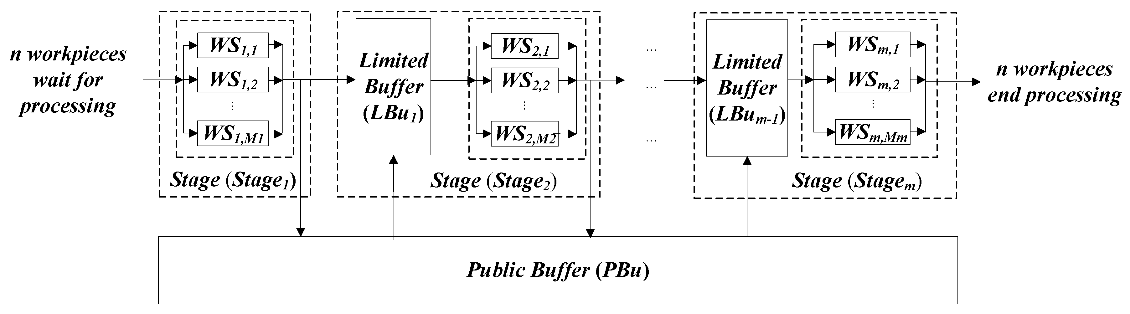
As shown in Figure 1, the FFSP–PB could be described as follows: $m$ stages in the workshop and the processing queues of $n$ workpieces need to be processed in order with $m$ processing stages. At least one of the $m$ stages consists of two or more parallel workstations, and the processing times of the workpiece are the same on different parallel workstations at one stage. A buffer with limited capacity is set up between stages; if the limited buffer capacity between stages reaches the upper limit, production blockage is likely to occur. In order to alleviate production blockage, a public buffer is set up in the production workshop, and this area provides services for all stages. If the capacity of the limited buffer between the stages reaches the upper limit, the workpiece can be moved into the public buffer for temporary storage. All workpieces are processed online from the first stage, completing all stages sequentially. If the capacity of the limited buffer between stages reaches the upper limit, the newly completed workpiece is transferred to the public buffer. Under certain conditions, the workpiece during transfer can also be returned to the limited buffer. If the workpiece in the limited buffer is moved to the workstation of the next stage for processing, the limited buffer will have an available space. Subsequently, the workpiece in the public buffer that should have accessed the limited buffer is transferred back to the limited buffer. The transit time between limited buffer and public buffer cannot be ignored. Under preconditions of the online sequence of the workpiece, the standard processing time for transferring the workpiece, the standard processing time of the workpiece at each stage and the online sequence is optimized by global optimization method, and the movement of the workpiece among the workstation, the limited buffer, and the public buffer is controlled by the local scheduling rules. Thus, the scheduling results of the processing workstations, the start time, and the completion time of all workpieces at each stage and the information of the transport process are obtained.

2.2. Parameters in the Model

The parameters used in this study are as follows:

• $n$: Total number of workpieces to be processed;
• $m$: Total number of stages;
• $W{p}_i$: Workpiece $i$, $i\in \left\{1,\dots ,n\right\}$;
• $Stag{e}_j$: Stage $j$, $j\in \left\{1,\dots ,m\right\}$;
• $M_j$: Total number of workstations in stage $Stag{e}_j$, $j\in \left\{1,\dots ,m\right\}$;
• $W{S}_{j,l}$: Workstation $l$ of stage $Stag{e}_j$, $j\in \left\{1,\dots ,m\right\}$, $l\in \left\{1,\dots ,M_j\right\}$;
• $LB{u}_j$: Limited buffer of stage $Stag{e}_j$, $j\in \left\{2,\dots ,m\right\}$;
• $K{l}_j$: Maximum buffer capacity in the limited buffer $LB{u}_j$ of stage $Stag{e}_j$, $j\in \left\{1,\dots ,m\right\}$;
• $B{l}_{j,k}$: Buffer position $k$ of limited buffer $LB{u}_j$, $j\in \left\{2,\dots ,m\right\}$, $k\in \left\{1,\dots ,K{l}_j\right\}$;
• $WA{l}_j\left(t\right)$: At the $t$ time, the workpieces in the limited buffer $LB{u}_j$;
• $PBu$: Public buffer;
• $Kp$: Maximum buffer capacity in the public buffer $PBu$, $1\le Kp\le n-\min \left\{K{l}_j\right\}$;
• $T{s}_{i,j}$: The start time of the workpiece $W{p}_i$ at stage $Stag{e}_j$, $j\in \left\{1,\dots ,m\right\}$;
• $T{c}_{i,j}$: The completion time of the workpiece $W{p}_i$ at stage $Stag{e}_j$, $j\in \left\{1,\dots ,m\right\}$;
• $T{b}_{i,j}$: The standard processing time of the workpiece $W{p}_i$ at stage $Stag{e}_j$, $j\in \left\{1,\dots ,m\right\}$;
• $T{i}_{i,j}$: The entry time of the workpiece $W{p}_i$ into stage $Stag{e}_j$, $j\in \left\{1,\dots ,m\right\}$;
• $T{o}_{i,j}$: The departure time of the workpiece $W{p}_i$ out of stage $Stag{e}_j$, $j\in \left\{1,\dots ,m\right\}$;
• $Tl{i}_{i,j}$: The entry time of the workpiece $W{p}_i$ into limited buffer $LB{u}_j$, $j\in \left\{2,\dots ,m\right\}$;
• $Tl{o}_{i,j}$: The departure time of the workpiece $W{p}_i$ out of limited buffer $LB{u}_j$, $j\in \left\{2,\dots ,m\right\}$;
• $Tp{i}_{i,j}$: The entry time of the workpiece $W{p}_i$ into public buffer $PBu$ at stage $Stag{e}_j$, $j\in \left\{2,\dots ,m\right\}$;
• $Tp{o}_{i,j}$: The departure time of the workpiece $W{p}_i$ out of public buffer $PBu$ at stage $Stag{e}_j$, $j\in \left\{2,\dots ,m\right\}$;
• $Tbt$: The standard processing time for transferring the workpiece;
• $R{p}_i$: The workpiece $W{p}_i$ is on the way from the workstation to the public buffer;
• $R{l}_i$: The workpiece $W{p}_i$ is on the way from the public buffer to the limited buffer;
• $R{b}_i$: The workpiece $W{p}_i$ is on the way back to the limited buffer;
• $Cfp$: The time for electric flat carriage to finish the current task and return to the public buffer;
• $Tt{w}_{i,j}(t)$: At the $t$ time, the transit time of the workpiece $W{p}_i$ from the workstation of stage $Stag{e}_j$ to the public buffer.

2.3. Constraints

The variables used in this study and the constraints that exist between variables are as follows:

2.3.1. Assumptions

$$A{t}_{i,j,l}=\{\begin{array}{cc}1& \mathrm{Workpiece}W{p}_i\mathrm{is}\mathrm{assigned}\mathrm{to}\mathrm{be}\mathrm{processed}\mathrm{on}\mathrm{workstation}W{S}_{j,l}\\ 0& \mathrm{Workpiece}W{p}_i\mathrm{is}\mathrm{not}\mathrm{assigned}\mathrm{to}\mathrm{be}\mathrm{processed}\mathrm{on}\mathrm{workstation}W{S}_{j,l}\end{array}$$

(1)

$$OA{l}_{i,j}\left(t\right)=\{\begin{array}{cc}1& \mathrm{At}\mathrm{time}t,\mathrm{workpiece}W{p}_i\mathrm{is}\mathrm{in}\mathrm{limited}\mathrm{buffer}LB{u}_j\\ 0& \mathrm{At}\mathrm{time}t,\mathrm{workpiece}W{p}_i\mathrm{is}\mathrm{not}\mathrm{in}\mathrm{limited}\mathrm{buffer}LB{u}_j\end{array}$$

(2)

$$OA{p}_{i,j}\left(t\right)=\{\begin{array}{cc}1& \begin{array}{l}\mathrm{At}\mathrm{time}t,\mathrm{workpiece}W{p}_i\mathrm{that}\mathrm{should}\mathrm{have}\mathrm{entered}\\ \mathrm{limited}\mathrm{buffer}LB{u}_j\mathrm{is}\mathrm{in}\mathrm{public}\mathrm{buffer}\end{array}\\ 0& \begin{array}{l}\mathrm{At}\mathrm{time}t,\mathrm{workpiece}W{p}_i\mathrm{that}\mathrm{should}\mathrm{have}\mathrm{entered}\\ \mathrm{limited}\mathrm{buffer}LB{u}_j\mathrm{is}\mathrm{not}\mathrm{in}\mathrm{public}\mathrm{buffer}\end{array}\end{array}$$

(3)

$$OA{t}_{i,j}\left(t\right)=\{\begin{array}{cc}1& \begin{array}{l}\mathrm{At}\mathrm{time}t,\mathrm{workpiece}W{p}_i\mathrm{that}\mathrm{should}\mathrm{have}\\ \mathrm{entered}\mathrm{limited}\mathrm{buffer}LB{u}_j\mathrm{is}\mathrm{in}\mathrm{transit}\end{array}\\ 0& \begin{array}{l}\mathrm{At}\mathrm{time}t,\mathrm{workpiece}W{p}_i\mathrm{that}\mathrm{should}\mathrm{have}\\ \mathrm{entered}\mathrm{limited}\mathrm{buffer}LB{u}_j\mathrm{is}\mathrm{not}\mathrm{in}\mathrm{transit}\end{array}\end{array}$$

(4)

$$Pan\_Car\left(t\right)=\{\begin{array}{cc}0& \mathrm{At}\mathrm{time}t,\mathrm{electric}\mathrm{flat}\mathrm{carriage}\mathrm{is}\mathrm{on}\mathrm{workstation}\\ 1& \mathrm{At}\mathrm{time}t,\mathrm{electric}\mathrm{flat}\mathrm{carriage}\mathrm{is}\mathrm{in}\mathrm{limited}\mathrm{buffer}\\ 2& \mathrm{At}\mathrm{time}t,\mathrm{electric}\mathrm{flat}\mathrm{carriage}\mathrm{is}\mathrm{in}\mathrm{public}\mathrm{buffer}\\ 3& \begin{array}{l}\mathrm{At}\mathrm{time}t,\mathrm{electric}\mathrm{flat}\mathrm{carriage}\mathrm{is}\mathrm{in}\mathrm{transit}\mathrm{from}\\ \mathrm{workstation}\mathrm{to}\mathrm{public}\mathrm{buffer}\end{array}\\ 4& \begin{array}{l}\mathrm{At}\mathrm{time}t,\mathrm{electric}\mathrm{flat}\mathrm{carriage}\mathrm{is}\mathrm{in}\mathrm{transit}\mathrm{from}\\ \mathrm{public}\mathrm{buffer}\mathrm{to}\mathrm{limited}\mathrm{buffer}\end{array}\end{array}$$

(5)

2.3.2. General Constraint of Flexible Flow Shops Scheduling

$${\displaystyle \sum _{l=1}^{M_j}A{t}_{i,j,l}}=1,i\in \left\{1,\dots ,n\right\},j\in \left\{1,\dots ,m\right\}$$

(6)

$$T{c}_{i,j}=T{s}_{i,j}+T{b}_{i,j},i\in \left\{1,\dots ,n\right\},j\in \left\{1,\dots ,m\right\}$$

(7)

$$T{c}_{i,j-1}\le T{s}_{i,j},i\in \left\{1,\dots ,n\right\},j\in \left\{2,\cdots ,m\right\}$$

(8)

Equation (6) indicates that the constraint that the workpiece $W{p}_i$ can only be processed at one workstation of the stage $Stag{e}_j$ during the processing. Equation (7) indicates the constraints that the completion time of the workpiece $W{p}_i$ in the stage $Stag{e}_j$ is equal to the sum of its start time and standard processing time in the stage $Stag{e}_j$, which guarantees close machining between the workpieces. Equation (8) indicates the constraint that the workpiece $W{p}_i$ needs to complete the processing task of the current stage before the processing task of the next stage. This constraint limits the processing sequence of each workpiece in all stages. Equations (6)–(8) ensure that the whole processing is in accordance with the processing characteristics of the flexible flow shop.

2.3.3. Constraints of the Limited Buffers

$$Tl{i}_{i,j}\ge T{c}_{i,j-1},j\in \left\{2,\dots ,m\right\}$$

(9)

Equation (9) indicates the constraint that time $Tl{i}_{i,j}$ for the workpiece to enter the limited buffer $LB{u}_j$ cannot be less than the completion time $T{c}_{i,j-1}$ of this workpiece processed at the previous stage $Stag{e}_{j-1}$.

$$WA{l}_j\left(t\right)=\left\{J_i|OA{l}_{i,j}\left(t\right)=1\right\}$$

(10)

Equation (10) indicates the constraint and the workpieces in the limited buffer $LB{u}_j$ at the $t$ time.

$$card\left(WA{l}_j\left(t\right)\right)\le K{l}_j$$

(11)

Equation (11) indicates the constraint that at any time, the total number of workpieces in the collection $WA{l}_j$ waiting to be processed cannot be greater than the maximum buffer capacity $K{l}_j$ in the limited buffer. This constraint guarantees that the characteristics of the limited buffer correspond to the actual processing.

$$Tl{o}_{i,j}\ge Tl{i}_{i,j},j\in \left\{2,\dots ,m\right\}$$

(12)

Equation (12) denotes that time for the workpiece to leave the limited buffer $LB{u}_j$ cannot be less than the time for the workpiece to enter the limited buffer $LB{u}_j$.

2.3.4. Constraints of the Public Buffer

$$Tp{o}_{i,j}\ge Tp{i}_{i,j},j\in \left\{2,3,\dots ,m\right\}$$

(13)

Equation (13) indicates the time for the workpiece in the public buffer $PBu$ that should have entered the limited buffer $LB{u}_j$ to leave the public buffer $PBu$ should not be less than the time for it to enter the public buffer $PBu$. This constraint ensures that the moving in and out of the public buffer conforms to the actual processing.

$$WA{p}_j\left(t\right)=\left\{W{p}_i|OA{p}_{i,j}\left(t\right)=1\right\}$$

(14)

Equation (14) represents the collection of all workpieces contained in the public buffer $PBu$ at time $t$.

$$card\left(WA{p}_j\left(t\right)\right)\le Kp$$

(15)

Equation (15) indicates the constraint that at any time, the sum of workpieces contained in the to-be-processed collection $WA{p}_j$ is less than or equal to the maximum buffer capacity $Kp$ of the public buffer. This constraint guarantees that the characteristics of the public buffer conform to the actual processing.

$$Tt{w}_{i,j}(t)=(t-T{o}_{i,j})$$

(16)

Equation (16) shows that at time t, the time for the workpiece $W{p}_i$ to be transferred from the workstation of the stage $Stag{e}_j$ to the public buffer is equal to the difference between the time for the workpiece $W{p}_i$ to leave the workstation of stage $Stag{e}_j$ at time $t$.

$$Tt{w}_{i,j}(t)\le Tbt$$

(17)

Equation (17) indicates the constraint that at time $t$, the time for the workpiece $W{p}_i$ to be transferred from the workstation of the stage $Stag{e}_j$ to the public buffer should be less than the standard processing time for transferring the workpiece.

2.3.5. Other Constraints

(1)

Continuous processing constraint: If the workpiece has started the processing task of a certain stage, it cannot be interrupted until the task is completed.

(2)

Workstation uniqueness constraint: A workstation can only process one workpiece simultaneously.

(3)

Workstation availability constraint: All workstations are available at the scheduling time.

(4)

Time simplification constraint: Irrespective of the transit time of the workpiece between the limited buffer and workstation, only the processing time of the workpiece at each stage and the transit time of the workpiece on the electric flat carriage are considered.

3. Research on FFSP–PB Local Scheduling Rules

During production, when the limited buffer capacity of the current stage reaches the upper limit, the finished workpiece of the previous stage is directly transferred to the public buffer. The available workstation at this stage allows the processing of the workpiece in limited buffer at the current stage. Strikingly, there is available space in the limited buffer at this stage. If the workpiece is directly transferred from the public buffer to the limited buffer of the current stage, the available space would not be occupied by the finished workpiece of the previous stage during the period when the workpiece is transported back to the limited buffer of the current stage; otherwise, the workpiece transferred from the public buffer will collide with the completed workpiece of the previous stage while entering the available space. In order to prevent this conflict and as long as the workpiece in the public buffer starts to be transported to the available space in the limited buffer of the current stage, this space cannot be occupied, which might block the finished workpiece of the previous stage at its processing workstation. According to the above analysis, after adding the public buffer to the workshop, if the corresponding local scheduling rules are not established, the production blockage and completion time of gross workpieces cannot be reduced effectively. In order to play the role of public buffer and further alleviate the production blockage, the reentrant rules of the electric flat carriage and the workpiece transfer rules in the public buffer are designed. These local heuristics rules can control the transit of the workpiece among limited buffer, public buffer, and workstation. These rules exert the role of public buffer to reduce the production blockage.

3.1. Reentrant Rules of Electric Flat Carriage

At time $t$, if there is available space in the limited buffer $LB{u}_{j+1}$ and workpieces that have completed the processing task of stage $Stag{e}_j$ and transferred to public buffer $PBu$, the already-spent transit time $Tt{w}_{i,j}(t)$ of the workpiece in transit will be compared to the estimated minimum completion time $\min \left\{\left(T{c}_{i,j}-t\right)|\left(T{s}_{i,j}-t\right)\le 0,\left(T{c}_{i,j}-t\right)>0\right\}$ of all workpieces at the current stage $Stag{e}_j$. If the estimated minimum completion time is longer than the already-spent transit time of the workpiece, the electric flat carriage will begin to turn back, transporting the workpiece back to the limited buffer $LB{u}_{j+1}$ of the next stage $Stag{e}_{j+1}$.

At time $t$, if $card\left(OA{l}_{i,j+1}\left(t\right)\right)<K{l}_{j+1}$ & $OA{t}_{i,j+1}\left(t\right)\cdot Tt{w}_{i,j}(t)<\min \left\{\left(T{c}_{i,j}-t\right)|\left(T{s}_{i,j}-t\right)\le 0,\left(T{c}_{i,j}-t\right)>0\right\}$ & $Pan\_Car\left(t\right)=3$ & $OA{t}_{i,j+1}\left(t\right)\ne 0$, the workpiece begins to be transported, and the state of electric flat carriage becomes $Pan\_Car\left(t\right)=4$.

3.2. Workpiece Transfer Rules in Public Buffer

At time $t$, there is available space in the limited buffer $LB{u}_{j+1}$ and workpieces in the public buffer that should have entered the limited buffer $LB{u}_{j+1}$. If the electric flat carriage is in the public buffer $Pan\_Car\left(t\right)=2$, the standard processing time for transferring the workpiece $Tbt$ will be compared to the estimated minimum completion time $\min \left\{\left(T{c}_{i,j}-t\right)|\left(T{s}_{i,j}-t\right)\le 0,\left(T{c}_{i,j}-t\right)>0\right\}$ of all workpieces at stage $Stag{e}_j$. If the estimated minimum completion time is longer than the standard processing time for transferring the workpiece, the workpieces currently in the public buffer $PBu$ that should have entered the limited buffer $LB{u}_{j+1}$ are transported back to the limited buffer $LB{u}_{j+1}$; however, if the estimated minimum completion time is short, the available space in the limited buffer $LB{u}_{j+1}$ will remain idle until the workpiece with the estimated minimum completion time at the current stage is accessed.

If the electric flat carriage is not in the public buffer, i.e., $Pan\_Car\left(t\right)\ne 2$, the sum of the standard processing time for transferring the workpiece $Tbt$ and the time $Cfp$ for electric flat carriage to the public buffer after completing the current task will be compared to the estimated minimum completion time $\min \left\{\left(T{c}_{i,j}-t\right)|\left(T{s}_{i,j}-t\right)\le 0,\left(T{c}_{i,j}-t\right)>0\right\}$ of all workpieces at stage $Stag{e}_j$. If the estimated minimum completion time is longer than that described above, the workpieces currently in the public buffer $PBu$ that should have entered the limited buffer $LB{u}_{j+1}$ are transported back to the limited buffer $LB{u}_{j+1}$. If the estimated minimum completion time is shorter than that mentioned above, the available space in the limited buffer $LB{u}_{j+1}$ will remain idle until the workpiece with the estimated minimum completion time at the current stage is processed and accessed.

At time $t$, if $card\left(OA{l}_{i,j+1}\left(t\right)\right)<K{l}_{j+1}$ & $OA{p}_{i,j+1}\left(t\right)\cdot Tbt<\min \left\{\left(T{c}_{i,j}-t\right)|\left(T{s}_{i,j}-t\right)\le 0,\left(T{c}_{i,j}-t\right)>0\right\}$ & $Pan\_Car\left(t\right)=2$ & $OA{p}_{i,j+1}\left(t\right)\ne 0$, the workpiece begins to be transported, and the state of electric flat carriage becomes $Pan\_Car\left(t\right)=4$.

At time $t$, if $card\left(OA{l}_{i,j+1}\left(t\right)\right)<K{l}_{j+1}$ & $OA{p}_{i,j+1}\left(t\right)\cdot Tbt+Cfp<\min \left\{\left(T{c}_{i,j}-t\right)|\left(T{s}_{i,j}-t\right)\le 0,\left(T{c}_{i,j}-t\right)>0\right\}$ & $Pan\_Car\left(t\right)\ne 2$ & $OA{p}_{i,j+1}\left(t\right)\ne 0$, the workpiece begins to be transported, and the state of electric flat carriage becomes $Pan\_Car\left(t\right)=2$ after time $Cfp$.

4. Local Scheduling Rules for Multi-Queue Limited Buffers

In this study, HNN is primarily used for optimization. The energy function in the continuous HNN is monotonically decreasing, and the gradually decreasing process of the energy function is the process of neural network optimization. The algorithm employs this feature to solve the optimization problem and search for the optimal solution [27].

When the standard HNN algorithm solves the NP-hard problem, it establishes a non-linear correlation between the input and output of the network, since the activation function of the analog neurons in the neural network is a non-linear transfer function. Moreover, the output of the problem solution is a non-linear space, which might encompass multiple poles, renders the algorithm as an optimal local solution in the event of failure to obtain the optimal global solution. Also, the algorithm cannot break after falling into local extremum, which makes the overall evolutionary trend irreversible. Thus, the simulated annealing algorithm is introduced into the standard HNN algorithm to prevent its premature convergence, expand the search ability of the feasible solution, and improve the global optimization effect.

4.1. HNN Algorithm

4.1.1. Establishing the Permutation Matrix

The permutation matrix is a bridge connecting the buffer dynamic capacity-increase problem in a flexible flow shop with public buffer and the improved HNN algorithm. This study applied the workpiece processing sequence in the first stage to construct the matrix. For example, the FFSP permutation matrix of the six workpieces to be processed is shown in

Table 1. FFSP permutation matrix of six workpieces.

Workpiece	Processing Sequence
	1	2	3	4	5	6
$W{p}_1$	0	1	0	0	0	0
$W{p}_2$	1	0	0	0	0	0
$W{p}_3$	0	0	0	1	0	0
$W{p}_4$	0	0	0	0	1	0
$W{p}_5$	0	0	1	0	0	0
$W{p}_6$	0	0	0	0	0	1

. The permutation matrix in

Table 2. Algorithm test result.

Example	LB	ICA			CGA			HNN			SAA–HNN
		$\overline{{\mathit{C}}_{\mathit{m}\mathit{a}\mathit{x}}}$	$\mathit{A}\mathit{R}\mathit{E}$	$\overline{\mathit{T}\mathit{i}\mathit{m}\mathit{e}}$	$\overline{{\mathit{C}}_{\mathit{m}\mathit{a}\mathit{x}}}$	$\mathit{A}\mathit{R}\mathit{E}$	$\overline{\mathit{T}\mathit{i}\mathit{m}\mathit{e}}$	$\overline{{\mathit{C}}_{\mathit{m}\mathit{a}\mathit{x}}}$	$\mathit{A}\mathit{R}\mathit{E}$	$\overline{\mathit{T}\mathit{i}\mathit{m}\mathit{e}}$	$\overline{{\mathit{C}}_{\mathit{m}\mathit{a}\mathit{x}}}$	$\mathit{A}\mathit{R}\mathit{E}$	$\overline{\mathit{T}\mathit{i}\mathit{m}\mathit{e}}$
j15c5c1	85	91.3	7.4%	6.6 s	90.2	6.1%	6.3 s	97.3	14.5%	3.5 s	90.1	6.1%	4.1 s
j15c5c2	90	102.1	13.5%	6.7 s	99.9	11.0%	6.4 s	109.6	21.8%	3.7 s	96.7	7.4%	4.6 s
j15c5d1	167	206.4	23.6%	6.9 s	204.2	22.3%	6.6 s	242.1	45.0%	4.1 s	190.7	14.2%	4.8 s
j15c5d2	82	101.3	23.6%	6.7 s	96.9	18.2%	6.4 s	111.8	36.4%	3.8 s	92.1	12.3%	4.5 s
j80c4a1	—	1415.4	—	24.3 s	1389.5	—	29.5 s	1453.7	—	6.5 s	1375.9	—	7.7 s
j80c4a2	—	1434.7	—	21.1 s	1419.4	—	24.5 s	1474.2	—	6.1 s	1408.3	—	6.2 s
j80c8a1	—	2088.4	—	24.2 s	2027.2	—	26.4 s	2170.2	—	6.4 s	2011.2	—	7.5 s
j80c8a2	—	1856.4	—	24.5 s	1827.7	—	24.4 s	1956.6	—	5.8 s	1811.1	—	7.5 s
j120c20a1	—	3764.7	—	44.6 s	3699.1	—	48.3 s	3954.9	—	13.9 s	3442.5	—	14.8 s
j200c10a1	—	4953.2	—	76.3 s	4787.8	—	79.7 s	5211.5	—	18.6 s	4364.9	—	21.5 s

indicates the processing sequence of the six workpieces $\left\{W{p}_2,W{p}_1,W{p}_5,W{p}_3,W{p}_4,W{p}_6\right\}$.

4.1.2. Establishing the Energy Function

As a major feedback of the network, the energy function can easily determine the stability of the system.

(1) Energy function row constraint

$$E_1=\frac{A}{2}{\displaystyle \sum _{x=1}^n{\displaystyle \sum _{i=1}^{n-1}{\displaystyle \sum _{j=i+1}^n{V}_{xi}}}}{V}_{xj}=0$$

(18)

Equation (18) indicates that the sum ${\displaystyle \sum _{x=1}^n{\displaystyle \sum _{i=1}^{n-1}{\displaystyle \sum _{j=i+1}^n{V}_{xi}}}}{V}_{xj}$ of all elements of $n$ rows multiplied by each other in order should be 0, i.e., each row in the FFSP permutation matrix only has one ‘1’, indicating that a workpiece can only be processed once at each stage. $V_{xi}$ represents the element of the $i$ column of the $x$ row of the FFSP permutation matrix, and $A$ is the coefficient.

(2) Energy function column constraint

$$E_2=\frac{B}{2}{\displaystyle \sum _{i=1}^n{\displaystyle \sum _{x=1}^{n-1}{\displaystyle \sum _{y=x+1}^n{V}_{xi}}}}{V}_{yi}=0$$

(19)

Equation (19) denotes that the sum ${\displaystyle \sum _{i=1}^n{\displaystyle \sum _{x=1}^{n-1}{\displaystyle \sum _{y=x+1}^n{V}_{xi}}}}{V}_{yi}$ of all elements of $n$ columns multiplied by each other in a specific order should be 0, i.e., each column in the FFSP permutation matrix only has one ‘1’, indicating that a workpiece can only be processed once at one stage, and $B$ is the coefficient.

(3) Energy function overall constraint

$$E_3=\frac{C}{2}{\left({\displaystyle \sum _{i=1}^n{\displaystyle \sum _{x=1}^n{V}_{xi}}}-n\right)}^2$$

(20)

Equation (20) indicates that the sum ${\displaystyle \sum _{i=1}^n{\displaystyle \sum _{x=1}^n{V}_{xi}}}-n$ of all elements should be 0, i.e., there are $n$ ‘1’ in the FFSP permutation matrix, indicating that all workpieces are to be processed at one stage. In the Equation, $C$ is the coefficient, and the square value is used to conform to the expression of energy, as well as embody a punishment for not meeting the constraint.

(4) Energy function target item

Since the main optimization goal of the FFSP–PB is the makespan, the fourth item of the energy function needs to be expressed in combination with the makespan, as shown in Equation (21), and $D$ is the coefficient.

$$E_4=\frac{D}{2}{C}_{\max }$$

(21)

Combining Equations (18)–(21), the energy function for constructing FFSP–PB is as follows:

$$E=\frac{A}{2}{E}_1+\frac{B}{2}{E}_2+\frac{C}{2}{E}_3+\frac{D}{2}{E}_4=\frac{A}{2}{\displaystyle \sum _{x=1}^n{\displaystyle \sum _{i=1}^{n-1}{\displaystyle \sum _{j=i+1}^n{V}_{xi}}}}{V}_{xj}+\frac{B}{2}{\displaystyle \sum _{i=1}^n{\displaystyle \sum _{x=1}^{n-1}{\displaystyle \sum _{y=x+1}^n{V}_{xi}}}}{V}_{yi}+\frac{C}{2}{\left({\displaystyle \sum _{i=1}^n{\displaystyle \sum _{x=1}^n{V}_{xi}}}-n\right)}^2+\frac{D}{2}{C}_{\max }$$

(22)

According to a previous study [26], Equation (22) can be improved to:

$$E=\frac{A}{2}{\displaystyle \sum _{x=1}^n{\left({\displaystyle \sum _{i=1}^n{V}_{xi}}-1\right)}^2}+\frac{B}{2}{\displaystyle \sum _{i=1}^n{\left({\displaystyle \sum _{x=1}^n{V}_{xi}}-1\right)}^2}+D{C}_{\max }$$

(23)

To ensure the symmetry for the solution of HNN algorithm, the value of $A$ in Equation (23) needs to be equal to the value of $B$.

4.1.3. Establishing HNN Dynamic Differential Equation

According to another study [27], the connection weight coefficient is calculated as follows:

$$\frac{d{u}_{xi}}{dt}=-\frac{\partial E}{\partial V_{xi}}$$

(24)

Equations (23) and (24) can derive HNN dynamic equation as follows:

$$\frac{d{u}_{xi}}{dt}=-A\left({\displaystyle \sum _{i=1}^n{V}_{xi}-1}\right)-A\left({\displaystyle \sum _{y=1}^n{V}_{yi}-1}\right)$$

(25)

The correlation function between input $u_{xi}$ and output $V_{xi}$ of the simulating neuron in HNN algorithm is:

$$V_{xi}\left(t_0\right)={\phi }_{xi}\left(u_{xi}\right)=\frac{1}{2}\left[1+\tanh \left(\frac{u_{xi}\left(t_0\right)}{u_0}\right)\right]$$

(26)

According to the HNN dynamic equation, the input bias $\Delta u_{xi}$ is:

$$\Delta u_{xi}\left(t_0\right)=\frac{d{u}_{xi}}{dt}{V}_{yj}$$

(27)

In the evolution process of HNN, the input is updated by the first-order Euler Equation, which is shown in Equation (28):

$$u_{xi}\left(t_0+\Delta t\right)=u_{xi}\left(t_0\right)+{\frac{d{u}_{xi}}{dt}|}_{t=t_0}\Delta t$$

(28)

4.2. Improvement of the HNN Algorithm

Since the energy function of the standard HNN algorithm decreases monotonically, the optimization range of the algorithm is narrow with a fixed optimization direction, which ultimately leads the algorithm to easily fall into a local extremum and is difficult to jump out. The idea of the simulated annealing algorithm exists between the given solution and the new solution is generated in the local area by the given solution. The solution with the better fitness is accepted by Metropolis acceptance criteria [28], while the solution with the poorer fitness is selected to expand the searching range of the solution space. Therefore, in the process of optimizing the standard HNN algorithm, the idea of the simulated annealing algorithm is introduced to expand the optimization range of the standard HNN algorithm and further achieve a better solution.

After the standard HNN algorithm is introduced, the idea of the simulated annealing algorithm during each training process of the standard HNN algorithm causes the neuron input to increase the random disturbance in the HNN algorithm after energy function value, which is computed. The energy function value of the HNN after disturbance input is computed. Energy function value of the original input is compared to the energy function value of the disturbance input; if the energy function value is smaller, it indicates that the value is better. If the original energy function value is not smaller than the energy function value of the disturbance input, the energy function value of the disturbance input is selected to replace the original energy function value, and then the HNN algorithm starts the next generation of optimization. If the original energy function value is smaller than the energy function value of the disturbance input, according to the Metropolis acceptance criteria, the energy value function of the disturbance input is compared to the original energy function value. If the Metropolis acceptance criteria are fulfilled, the energy function value of the disturbance input is chosen to replace the original energy function value, and then the HNN algorithm starts the next generation optimization. Otherwise, the original energy function value does not change and enters the next generation of optimization. After the above process of algorithm optimization is repeated several times, a part of the energy function does not show monotone decreasing characteristic during convergence. However, the global convergence trend of the energy function still shows a decreasing tendency and converges to the optimal equilibrium point. Finally, the ability of the standard HNN algorithm to jump out of local extremum is improved.

The main steps for the HNN algorithm based on the simulated annealing algorithm for solving the scheduling problem are as follows:

Step 1: Set the initial parameters $A,D,u_0,t_0,\Delta t$ of the HNN algorithm.

Step 2: Set the maximum generation $K_{\max }$ and the evolutionary generation $K=0$.

Step 3: Set the initial value of $u_{xi}(t_0)$, whose value is within the interval $\left[-1,1\right]$.

Step 4: Set the initial value of each element $V_{xi}$ in the network initial permutation matrix to 0.

Step 5: Calculate the output $V(t_0)$ of each neuron according to Equation (26), and judge whether the permutation matrix at this time point is valid. The validity of the permutation matrix needs to be judged strictly by the energy function constraint. If the permutation matrix is legal, the output is obtained, $C_{\max }$ is calculated, and continue to step 6; if not, return to step 2.

Step 6: Calculate the energy $E\left(t_0\right)$ of the network at this time point according to Equation (23).

Step 7: Calculate $\frac{d{u}_{xi}}{dt}$ according to Equation (24).

Step 8: Increase the random disturbance $\Delta t_0$ to the input of neuron $u_{xi}\left(t_0\right)$, and the neuron input changes into $u_{xi}\left(t_0+\Delta t_0\right)$ at this time. $u_{xi}\left(t_0+\Delta t_0\right)$ is calculated according to Equation (28), and the permutation matrix $V\left(t_0+\Delta t_0\right)$ is updated by $u_{xi}\left(t_0+\Delta t_0\right)$.

Step 9: Calculate the value of energy function in network $E\left(t_0+\Delta t\right)$ at this time.

Step 10: If $E\left(t_0+\Delta t_0\right)\le E\left(t_0\right)$, then $E\left(t_0\right)=E(t_0+\Delta t_0)$; if not, then judge whether the result satisfies the Metropolis acceptance criteria. If the criteria are fulfilled, then $E\left(t_0\right)=E(t_0+\Delta t_0)$; if not, then $E\left(t_0\right)=E(t_0)$.

Step 11: If the permutation matrix output is legal at this time, then continue to step 12, otherwise return to step 5. At the same time point, evolutionary generation $K$ is processed as $K=K+1$.

Step 12: If the iteration $K$ has reached the maximum generation $K_{\max }$ and the permutation matrix output is legal at this time point, then output the result, otherwise return to step 3.

The flowchart of the SAA–HNN algorithm is shown in Figure 2.

4.3. Optimization Performance Testing on the SAA–HNN Algorithm

In order to verify the effect of optimization performance of the HNN algorithm, which adds the idea of the simulated annealing algorithm in comparison to the optimization effect of the improved HNN algorithm and the typical algorithms of the swarm intelligence algorithm, four groups of small-scale FFSP standard example data and six groups of large-scale FFSP instance data were used to test and analyze the SAA–HNN algorithm and its comparison algorithms. The comparison algorithms included ICA, CGA, and HNN.

Four groups of small-scale FFSP standard example data and four groups of large-scale FFSP instance data were used to, respectively, test and analyze. Moreover, the SAA–HNN algorithm was compared to ICA, CGA, and HNN to verify the effect of optimization performance of HNN algorithm, which adds the idea of the simulated annealing algorithm.

The four groups of small-scale FFSP test data were from the standard examples [29,30] proposed by Neron and Taillard based on the standard FFSP, while six groups of large-scale FFSP test data adopted the actual production data. Each algorithm was run 30 times under each group of data, and the average makespan $\overline{C_{max}}$ was applied as the main evaluation index to obtain the result. In addition, the maximum evolution of the four algorithms was 500 generations. The test results are shown in Table 2.

In Table 2, the ‘j15c5c1’ standard example is taken as an example. ‘j15’ indicates that the total number of processed workpieces is 15. ‘c5’ indicates that the total number of processing stages is 5, and since there is only one machine per stage, the total number of machines is also 5. ‘c1’ represents the difficulty of the standard example. The easy-to-solve examples include six j10c10c* classes, i.e., the total examples of ‘a’ class and ‘b’ class. The hard-to-solve examples include the other ‘c’ classes, i.e., the total examples of ‘d’ class and ‘e’ class. $LB$ is the lower bound of the makespan of the standard example whose value has been given in the literature [31,32], and $ARE$ represents the average relative error of the solution obtained by this algorithm as compared to the lower bound of the makespan. The smaller the $ARE$, the better the optimization effect of the algorithm. $\overline{Time}$ means the average optimization time of the standard example; the smaller the $\overline{Time}$, the better the optimization speed of the algorithm.

According to the test results in Table 2, based on four groups of small-scale standard example data, in terms of optimization effect, $ARE$ between the ICA algorithm and the CGA algorithm is 7.4% and 6.1%, respectively, under j15c5c1 standard example data. Therefore, its optimization effect is improved. The $ARE$ of the HNN algorithm under j15c5c1 standard example data is 14.5%, which increases to 7.1% and 8.4% in comparison to ICA and CGA, respectively. So the optimization effect is relatively poor. The $ARE$ of the SAA–HNN algorithm is 6.1% under j15c5c1 standard example data and is smaller than those of the other three algorithms, so the optimizing effect of the SAA–HNN algorithm is relatively better. The other small-scale standard example data also show the same status. In terms of optimization time, ICA is similar to CGA in average optimization time, which is 6–7 s time range. However, the average optimization time of HNN algorithm is 3–4 s time range and is shortened to about 50% as much as ICA and CGA with obvious improvement in the optimization speed. Although average optimization time of the SAA–HNN algorithm increases about 0.5 s as much as the HNN algorithm, it retains high optimization speed. In terms of four groups of large-scale data, on the basis of optimization effect, the SAA–HNN algorithm increases about 4% as compared to the other three algorithms. However, in terms of optimization time, the optimization speed of the SAA–HNN algorithm accelerates about 70% as much as ICA and CGA.

Based on the above tests using four groups of small-scale data and six groups of large-scale data for four algorithms, the SAA–HNN algorithm has faster optimization speed than the comparison algorithms, with significantly improved evaluation index under small-scale data. Also, under large-scale data, the SAA–HNN algorithm still maintains a high speed of optimization, and the evaluation index is relatively better. Therefore, the SAA–HNN algorithm is suitable for solving large-scale and complicated scheduling optimization problems, and hence, has a broad applicability.

During the test, four algorithms were considered based on 30 simulation experiments with large-scale data. The makespan $C_{max}$ obtained at each time point exhibited obvious fluctuation. Since the HNN algorithm can easily fall into local extremum, its $C_{max}$ may appear as a large outlier. In order to compare and evaluate the optimization effect of the four algorithms on large-scale data, j80c8a2 data were considered as the example, and the $C_{max}$ values obtained by running four algorithms for 30 times are drawn into a box plot (Figure 3).

A box-plot is a statistical graph for describing the discrete degree of a group of data. The stability of the optimization effect can be reflected by the box-plot. The interquartile range $IQR$ was used to measure the discrete degree of the data in the box-plot.

As can be seen from Figure 3, the HNN algorithm generates three large outliers of 2033, 2047, and 2056, respectively, in the 30 running times of the algorithm, indicating that the HNN algorithm easily falls into the local extremum. The median of box-plot produced by the SAA–HNN algorithm is 1815, and other medians of box-plot produced by other algorithms are 1854, 1828, and 1956, respectively. Therefore, the box-plot of the SAA–HNN algorithm is in the lowest position, which indicates that the overall quality of the solution generated by the SAA–HNN algorithm is better than the other three algorithms. Besides, the $IQR$ of the box-plot generated by the SAA–HNN algorithm is 23, and the $IQR$ of the box-plot generated by the other three algorithms are 25, 46, and 38, respectively, indicating that the SAA–HNN algorithm produces the smallest discrete degree, and the stability of the scheduling results under large-scale data was optimal among the four algorithms.

Based on the above analysis, the SAA–HNN algorithm is better than the ICA, CGA, and HNN algorithms, and it also maintains fast optimization of the HNN algorithm in terms of optimization speed while solving the scheduling problem of small-scale and large-scale data. This indicates that the idea of the simulated annealing algorithm overcomes the HNN algorithm for falling into local extremum, and the SAA–HNN algorithm has a strong ability of continuous evolution.

5. FFSP–PB Instance Test

Taking a bus manufacturer in actual large-scale equipment manufacturing enterprises as an example, simulation data similar to the production operation of the body shop and paint shop for the bus manufacturer were constructed. The body shop of the bus manufacturer was a rigid flow shop with multiple production lines that could be simplified into one production stage. The paint shop could be simplified into three stages. Therefore, the simulation data included four stages: $\left\{Stag{e}_1,Stag{e}_2,Stag{e}_3,Stag{e}_4\right\}$. The parallel workstation of these four stages was $\left\{M_j\right\}$ = $\left\{3,3,3,3\right\}$. A limited buffer occurred between each stage, and the maximum capacity of each limited buffer was $\left\{LB{u}_2,LB{u}_3,LB{u}_4\right\}$ = $\left\{2,2,2\right\}$. In addition, a public buffer was set on the production line, and the standard processing time for transferring the workpiece $TBt$ was 5. The maximum buffer capacity in the public buffer was 3.

The simulation test first analyzed the impact of the relevant local scheduling rules for FFSP–PB on the scheduling results, and discussed the role of the public buffer and local scheduling rules for the public buffer in alleviating the production blockage and improving the scheduling results. Finally, the SAA–HNN algorithm and other global optimization algorithms were combined with the local scheduling rules, respectively, to solve the FFSP–PB problem under different data scales, which verified the optimization performance of the SAA–HNN algorithm with respect to the complex scheduling problems. Thus, the efficiency of the combination of the SAA–HNN algorithm and local scheduling rules for solving the FFSP–PB problem was assessed.

5.1. Evaluation Index of Scheduling Results

In order to better analyze and study the scheduling results during the scheduling process, we employed the makespan $C_{max}$ as the optimization goal, establishing other evaluation indexes related to the actual production, including the total workstation idle time $TWIT$, the total plant factor $TPF$, and total workpiece blockage time $TWBT$. Except for $TPF$, the smaller the value, the better the other evaluation indexes:

(1) Makespan

$$C_{max}=\max \left\{T{c}_{i,m}\right\},i\in \left\{1,\mathrm{\dots }n\right\}$$

(29)

In Equation (29), makespan $C_{max}$ indicates the maximum value of all workpieces that completed processing at the last stage.

(2) Total workstation idle time

$$TWIT={\displaystyle \sum _{j=1}^m{\displaystyle \sum _{l=1}^{M_j}\left(\left(\max \left\{T{o}_{i,j}\cdot A{t}_{i,j,l}\right\}-\min \left\{S_{i,j}\cdot A{t}_{i,j,l}\right\}\right)-{\displaystyle \sum _{i=1}^n\left(T{b}_{i,j}\cdot A{t}_{i,j,l}\right)}\right)}}$$

(30)

In Equation (30), $TWT$ represents the sum of the idle time for the workstation between the start time of the first processed workpiece and the completion time of the last processed workpiece.

(3) Total plant factor

$$TPF=\frac{{\displaystyle \sum _{j=1}^m{\displaystyle \sum _{i=1}^n\left(T{b}_{i,j}\right)}}}{{\displaystyle \sum _{j=1}^m{\displaystyle \sum _{i=1}^n{\displaystyle \sum _{l=1}^{M_j}\left(\max \left\{T{o}_{i,j}\cdot A{t}_{i,j,l}\right\}-\min \left\{S_{i,j}\cdot A{t}_{i,j,l}\right\}\right)}}}}$$

(31)

In Equation (31), $TPF$ represents the total plant factor of all workstations, which is the ratio of the effective processing time of all workstations to the occupied period of all workstations. This period starts from the first workpiece processed on the workstation at each stage to the last workpiece that leaves the workstation after completion [33].

(4) Total workpiece blockage time

$$TWBT={\displaystyle \sum _{i=1}^n{\displaystyle \sum _{j=2}^m\left(T{o}_{i,j-1}-C_{i,j-1}\right)}}$$

(32)

In Equation (32), $TWBT$ indicates the sum of blockage time of all workpieces stuck on the workstations since the limited buffer is full and the electric flat carriage is in transit during the production.

5.2. Instance Test of FFSP–PB Local Scheduling Rules

5.2.1. Simulation Scheme

In order to verify the efficiency of the public buffer in reducing the production blockage during the process of buffer dynamic capacity-increase in flexible flow shop and analyze the role of the relevant local scheduling rules for the public buffer, three groups of simulation schemes were designed to solve the flexible flow shop scheduling problem with the limited buffer. Scheme 1: There is no public buffer and no reentrant rules of electric flat carriage or workpiece transfer rules in the public buffer. Scheme 2: There is a public buffer and no reentrant rules of electric flat carriage or workpiece transfer rules in the public buffer. Scheme 3: There is a public buffer, reentrant rules of electric flat carriage, and workpiece transfer rules in the public buffer.

5.2.2. Simulation Results and Analysis

To obtain a better evaluation of the scheduling results, 30 different online sequences were randomly generated, and the values of the evaluation index were obtained through simulation tests. Moreover, the average values of each evaluation index for each scheme based on 30 different online sequences were calculated (

Table 3. Comparison of evaluation indexes for the three scheme scheduling results.

Scheme	Evaluation Index
	$\overline{{\mathit{C}}_{\mathit{m}\mathit{a}\mathit{x}}}$	$\overline{\mathit{T}\mathit{W}\mathit{I}\mathit{T}}$	$\overline{\mathit{T}\mathit{P}\mathit{F}}$	$\overline{\mathit{T}\mathit{W}\mathit{B}\mathit{T}}$
1	182.6	40.4	0.924	26.3
2	168.5	37.1	0.951	18.4
3	159.3	22.5	0.978	5.9
$IR(2/1)$	7.72%	8.17%	2.92%	30.04%
$IR(3/1)$	12.76%	44.31%	5.84%	77.57%
$IR(3/1)$	5.46%	39.35%	2.84%	67.93%

), and Equation (33) was established. $IR(A/B)$ indicates the improvement range of $A$ with respect to the designated evaluation index of $B$, and the meanings of $A$ and $B$ would be modified according to the actual situation.

$$IR(A/B)=\left|[(A-B)/B]\right|\times 100\%$$

(33)

As is shown in Table 3, the main evaluation index makespan $C_{max}$ and the total workpiece blockage time $TWBT$ of Scheme 2 with the public buffer decreases to 14.1 and 7.9, respectively, as compared to that of Scheme 1 without the public buffer, and the improvement is 7.72% and 30.04%, respectively. If production line has a public buffer but does not establish corresponding local scheduling rules, it might lead to new production blockage. Thus, the reentrant rules of electric flat carriage and workpiece transfer rules in the public buffer are established. The main evaluation index makespan $C_{max}$ and total workpiece blockage time $TWBT$ of the reentrant rules of electric flat carriage in Table 3 and workpiece transfer rules in the public buffer of Scheme 3 decreases to 9.2 and 12.5, respectively, as compared to that of Scheme 2 with the public buffer but without the corresponding local scheduling rules, and the improvement is 5.46% and 67.93%, respectively. Meanwhile, the other evaluation indexes are also improved. The above analysis indicates that the public buffer adds in the flexible flow shop and relevant local scheduling rules can be established in order to relieve the production blockage effectively.

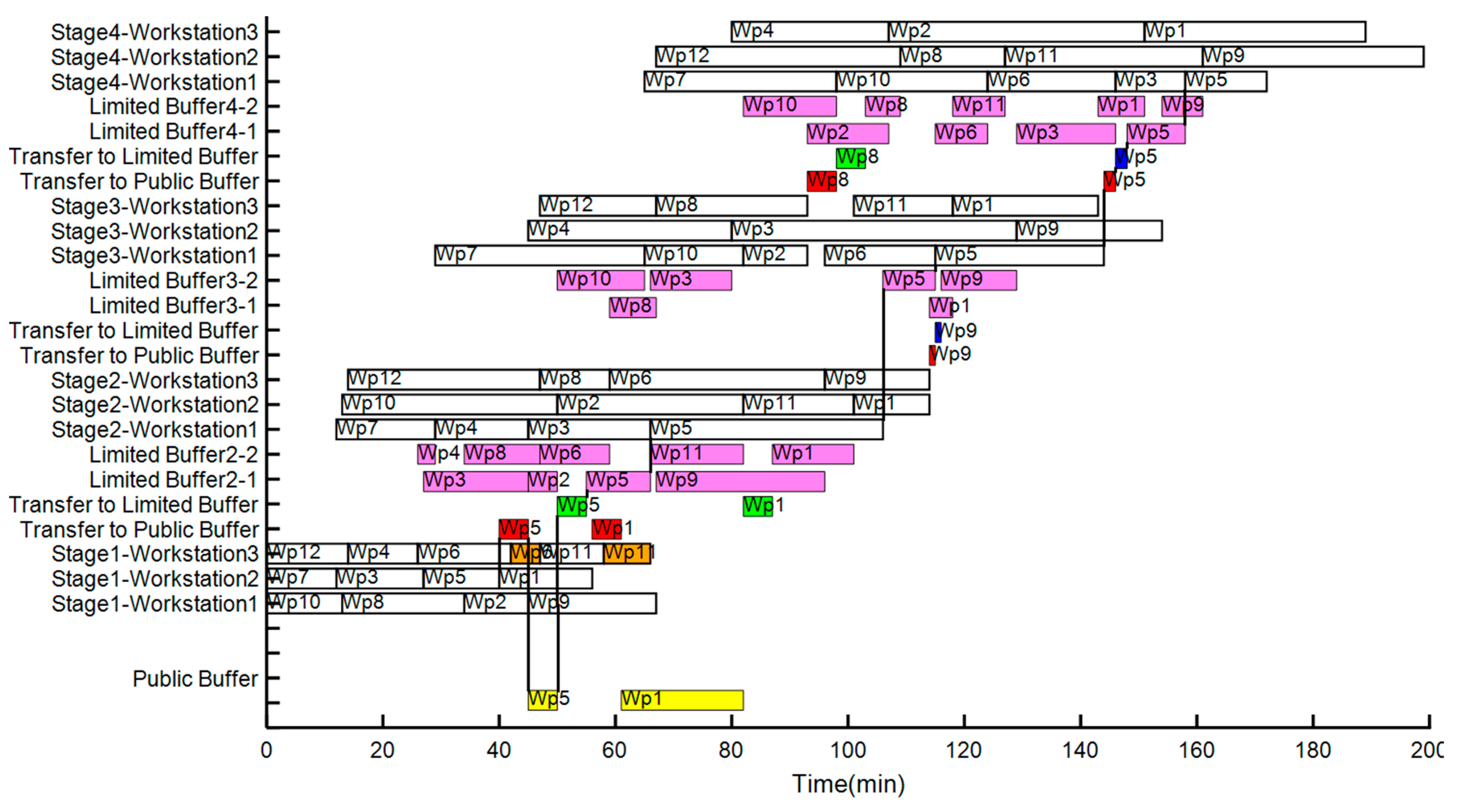
5.2.3. Gantt Chart Analysis of the Scheduling Result

Figure 4 shows the Gantt chart of the scheduling result of Scheme 3. The abscissa is the time axis, while the ordinate indicates the workstation of each stage, the limited buffer, and the public buffer. The violet part in the figure represents the time for the workpiece that is temporarily stored in the limited buffer; the red part indicates that the electric flat carriage transfers the workpiece from the workstation to the public buffer; the blue part indicates the time for the electric flat carriage that transfers the workpiece back to the limited buffer when transporting the workpiece from the workstation to the public buffer; the yellow part denotes that the workpiece is stored temporarily in the public buffer; the green part denotes that the electric flat carriage transports the workpiece from the public buffer to the limited buffer; the orange part in the figure represents the blockage time of the workpiece in the stage. Figure 4 demonstrates that restricted by Equation (6), the workpiece in each stage is processed only once at one workstation, and hence, the processing route of the workpiece $W{p}_5$ is $\left\{W{S}_{1,2},R{p}_5,PBu,R{l}_5,B{l}_{2,1},W{S}_{2,1},B{l}_{3,2},W{S}_{3,1},R{p}_5,R{b}_5,B{l}_{4,1},W{S}_{4,1}\right\}$, i.e., the processing route is represented by the connecting lines between the blocks in the figure.

At time $t$ = 40, the workpiece $W{p}_5$ completed the manufacturing task at workstation $W{S}_{1,2}$ of stage $Stag{e}_1$. Simultaneously, restricted by Equation (11), the limited buffer $LB{u}_2$ reached the upper limit of its capacity $WA{l}_2\left(40\right)=\left\{W{p}_3,W{p}_8\right\}$; thus, the workpiece $W{p}_5$ started to be transferred to the public buffer. At time $t$ = 45, the workpiece $W{p}_5$ entered the public buffer. At time $t$ = 50, the workpiece $W{p}_{10}$ completed the manufacturing task at workstation $W{S}_{2,2}$ of stage $Stag{e}_2$, and then left the workstation. The workpiece $W{p}_2$ entered the workstation $W{S}_{2,2}$ of stage $Stag{e}_2$, the space $B{l}_{2,1}$ in the limited buffer $LB{u}_2$ was available, and the workpiece $W{p}_5$ in the public buffer that should enter the limited buffer $LB{u}_2$ existed. Therefore, the workpiece transfer rules in the public buffer took effect. Since the electric flat carriage was at the position of the public buffer $Pan\_Car\left(50\right)=2$, the standard processing time for transferring the workpiece $Tbt=5$ was compared to the estimated minimum completion time $\min \left\{\left(T{c}_{i,1}-t\right)|\left(T{s}_{i,1}-t\right)\le 0,\left(T{c}_{i,1}-t\right)>0,i\in \left\{1,9,11\right\}\right\}$ = 6 for all workpieces at stage $Stag{e}_1$. Since the standard processing time for transferring the workpiece was less than the estimated minimum completion time for all workpieces of stage $Stag{e}_1$, the electric flat carriage transfered the workpiece $W{p}_5$ from the public buffer to the space $B{l}_{2,1}$ in the limited buffer $LB{u}_2$. At time $t$ = 55, the workpiece $W{p}_5$ entered the space $B{l}_{2,1}$ of the limited buffer $LB{u}_2$.

At time $t$ = 144, the workpiece $W{p}_5$ completed the manufacturing task at workstation $W{S}_{3,1}$ of stage $Stag{e}_3$. In addition, restricted by Equation (11), the limited buffer $LB{u}_4$ reached the upper limit of its capacity $WA{l}_4\left(144\right)=\left\{W{p}_1,W{p}_3\right\}$, following which, the workpiece $W{p}_5$ started to be transferred to the public buffer. At time $t$ = 146, the workpiece $W{p}_6$ completed the manufacturing task at workstation $W{S}_{4,1}$ of stage $Stag{e}_4$ and left the workstation. When the workpiece $W{p}_3$ entered the workstation $W{S}_{4,1}$ of stage $Stag{e}_4$, the space $B{l}_{4,1}$ in the limited buffer $LB{u}_4$ was available and the workpiece $W{p}_5$ was still in transportation $Pan\_Car\left(146\right)=3$, so the reentrant rules of the electric flat carriage took effect. Also, the already-spent transit time $Tt{w}_{5,3}(146)$ = 2 for transporting the workpiece $W{p}_5$ from the workstation of stage $Stag{e}_3$ to the public buffer was compared to the estimated minimum completion time $\min \left\{\left(T{c}_{i,4}-t\right)|\left(T{s}_{i,4}-t\right)\le 0,\left(T{c}_{i,4}-t\right)>0,i\in \left\{9\right\}\right\}$ = 8 for all workpieces at stage $Stag{e}_3$. Since the already-spent transit time of the workpiece $W{p}_5$ was less than the estimated minimum completion time for all workpieces of stage $Stag{e}_3$, the electric flat carriage returned the workpiece $W{p}_5$ to space $B{l}_{4,1}$ in the limited buffer $LB{u}_4$. Thus, at time $t$ = 148, the workpiece $W{p}_5$ entered the space $B{l}_{4,1}$ of the limited buffer $LB{u}_4$. Based on the above analysis, restricted by Equation (17), the already-spent transit time $Tt{w}_{5,3}(146)$ for transporting the workpiece $W{p}_5$ from the workstation of stage $Stag{e}_3$ to the public buffer should be less than the standard processing time for transferring workpiece.

From the above specific analysis of the Gantt chart about scheduling results, the reentrant rules of the electric flat carriage designed for the public buffer state that, when the workpiece is transferred to the public buffer, it should enter the available space in the limited buffer, following which, the workpiece reenters and is stored in the limited buffer to reduce its storage time in the public buffer and the total transfer time. Based on the workpiece transfer rules in public buffer, and in the event of available space in the limited buffer and that the workpiece transfers from the public buffer to the limited buffer and the previous stage of the limited buffer does not have the the completed workpiece, the workpiece in the public buffer is transferred to the available space in the limited buffer. This avoids competition for the available space in the limited buffer, which in turn, effectively reduces the new production blockage caused by the increase in the public buffer.

5.3. Instance Test of FFSP–PB Global Optimization Algorithm

5.3.1. Parameter Settings of the Optimization Algorithm

ICA, CGA, HNN, and SAA–HNN were utilized as global optimization algorithms. Moreover, these algorithms were combined with the reentrant rules of electric flat carriage and workpiece transfer rules in the public buffer designed for the public buffer to solve the FFSP–PB, which are optimal for comparing and analyzing the optimization performance and verifying its efficiency with local scheduling rules to resolve FFSP–PB. The parameter settings of the four global optimization algorithms are shown in

Table 4. Swarm evolutionary algorithm parameters.

Optimization Algorithm	Algorithm Parameter
ICA	Maximum evolutional generation $Gen$ = 500; number of imperialist countries $N_d$ = 5; number of colonial countries $N_z$ = 25; colonial impact factor $K$ = 0.15; similarity threshold $\alpha$ = 0.3.
CGA	Maximum evolutional generation $Gen$ = 500; number of populations $NP$ = 4; adjustment override of the learning rate $\beta$ = 0.08.
HNN	Maximum evolutional generations $Gen$ = 500; $A$ = 1.5; $D$ = 1; $u_0$ = 0.02; $\Delta t$ = 0.1
SAA–HNN	Maximum evolutional generations $Gen$ = 500; $A$ = 1.5; $D$ = 1; $u_0$ = 0.02; $\Delta t$ = 0.1; initial temperature $T_{max}$; end temperature $T_{min}$; cooling coefficient $b$.

.

5.3.2. Simulation Results and Analysis

(1) Evaluation Index of Scheduling Results

Each of the four algorithms were tested on the small-scale, medium-scale, and large-scale data. The total number $n$ of the processed workpieces was set to 12 in small-scale data, 40 in medium-scale data, and 80 in large-scale data.

i Small-scale data

The four algorithms were run 30 times for small-scale data, and the average values of the evaluation indexes obtained from 30 simulations are summarized in

Table 5. Comparison of the evaluation indexes of four algorithms’ scheduling results (small-scale data).

Algorithms	Evaluation Indexes
	$\overline{{\mathit{C}}_{\mathit{m}\mathit{a}\mathit{x}}}$	$\overline{\mathit{T}\mathit{W}\mathit{I}\mathit{T}}$	$\overline{\mathit{T}\mathit{P}\mathit{F}}$	$\overline{\mathit{T}\mathit{W}\mathit{B}\mathit{T}}$
ICA	176.54	46.42	0.931	27.42
CGA	157.89	39.56	0.952	22.17
HNN	189.55	47.32	0.927	33.30
SAA–HNN	129.92	22.59	0.978	9.89
$IR(\frac{SAA\text{-}HNN}{ICA})$	26.41%	51.34%	5.04%	63.93%
$IR(\frac{SAA\text{-}HNN}{CGA})$	17.71%	42.90%	2.73%	55.39%
$IR(\frac{SAA\text{-}HNN}{HNN})$	31.46%	52.26%	5.50%	70.3%

.

From the simulation results of small-scale data in Table 5, during the solving of FFSP–PB, the main evaluation index makespan $C_{max}$ of the SAA–HNN algorithm decreases to 46.62, 27.97, and 59.63 in comparison to the ICA, CGA, and HNN algorithms, respectively, and the improvement is 26.42%, 17.71%, and 31.46%, respectively. Moreover, the total workpiece blockage time $TWBT$ of the SAA–HNN algorithm decreases 17.53, 12.28, and 23.41 in comparison to the other three algorithms, respectively, and the improvement is 63.93%, 55.39%, and 70.3%, respectively. The total plant factor $TPF$ and total workstation idle time $TWBT$ also improves, thereby indicating that using the SAA–HNN algorithm as the global optimization algorithm to solve the FFSP–PB problem improves each evaluation index and reduces the production blockage in small-scale data simulation.

ii Medium-scale and large-scale data

The four algorithms were run 30 times for medium-scale and large-scale data, respectively, and the average values of the evaluation indexes obtained from the 30 simulations under the two data scales are listed in

Table 6. Comparison of the evaluation indexes of four algorithms’ scheduling results (medium-scale data).

Algorithms	Evaluation Indexes
	$\overline{{\mathit{C}}_{\mathit{m}\mathit{a}\mathit{x}}}$	$\overline{\mathit{T}\mathit{W}\mathit{I}\mathit{T}}$	$\overline{\mathit{T}\mathit{P}\mathit{F}}$	$\overline{\mathit{T}\mathit{W}\mathit{B}\mathit{T}}$
ICA	834.15	269.26	0.885	92.46
CGA	801.37	243.16	0.916	67.71
HNN	893.32	312.55	0.881	99.21
SAA–HNN	704.85	197.87	0.979	16.94
$IR(\frac{SAA\text{-}HNN}{ICA})$	15.50%	26.51%	10.62%	81.68%
$IR(\frac{SAA\text{-}HNN}{CGA})$	12.04%	18.63%	6.88%	74.24%
$IR(\frac{SAA\text{-}HNN}{HNN})$	21.10%	36.69%	11.12%	82.93%

and

Table 7. Comparison of the evaluation indexes of four algorithms’ scheduling results (large-scale data).

Algorithms	Evaluation Indexes
	$\overline{{\mathit{C}}_{\mathit{m}\mathit{a}\mathit{x}}}$	$\overline{\mathit{T}\mathit{W}\mathit{I}\mathit{T}}$	$\overline{\mathit{T}\mathit{P}\mathit{F}}$	$\overline{\mathit{T}\mathit{W}\mathit{B}\mathit{T}}$
ICA	1794.39	687.21	0.879	145.22
CGA	1650.60	582.57	0.899	106.06
HNN	1943.35	706.02	0.837	160.42
SAA–HNN	1379.16	462.18	0.982	25.15
$IR(\frac{SAA\text{-}HNN}{ICA})$	23.14%	32.75%	11.72%	82.68%
$IR(\frac{SAA\text{-}HNN}{CGA})$	16.44%	20.67%	9.23%	76.29%
$IR(\frac{SAA\text{-}HNN}{HNN})$	29.03%	34.54%	17.32%	84.32%

.

From the simulation results in Table 6 and Table 7, under medium-scale data, the main evaluation index makespan $C_{max}$ of the SAA–HNN algorithm decreases to 129.3, 96.52, and 188.47 in comparison to the ICA, CGA, and HNN algorithms, respectively, and the improvement is 15.50%, 12.04%, and 21.10%, respectively. Under large-scale data, the main evaluation index makespan $C_{max}$ of the SAA–HNN algorithm decreases to 415.23, 271.44, and 564.19 in comparison to the ICA, CGA and HNN algorithms, respectively, and the improvement is 23.14%, 16.44%, and 29.03%, respectively. Under medium-scale data and large-scale data, other evaluation indexes of the SAA–HNN algorithm also improve. The SAA–HNN algorithm performs optimally and has perfect adaptability during the solving of the FFSP–PB of medium-scale and large-scale data.

Based on the comprehensive analysis of the simulated results in the FFSP–PB of different data scales, it can be concluded that the SAA–HNN algorithm combines the reentrant rules of the electric flat carriage and workpiece transfer rules in the public buffer which are designed for the public buffer, effectively solves the FFSP–PB, and reduces the production blockage.

(2) Scheduling Evolutionary Process Analysis

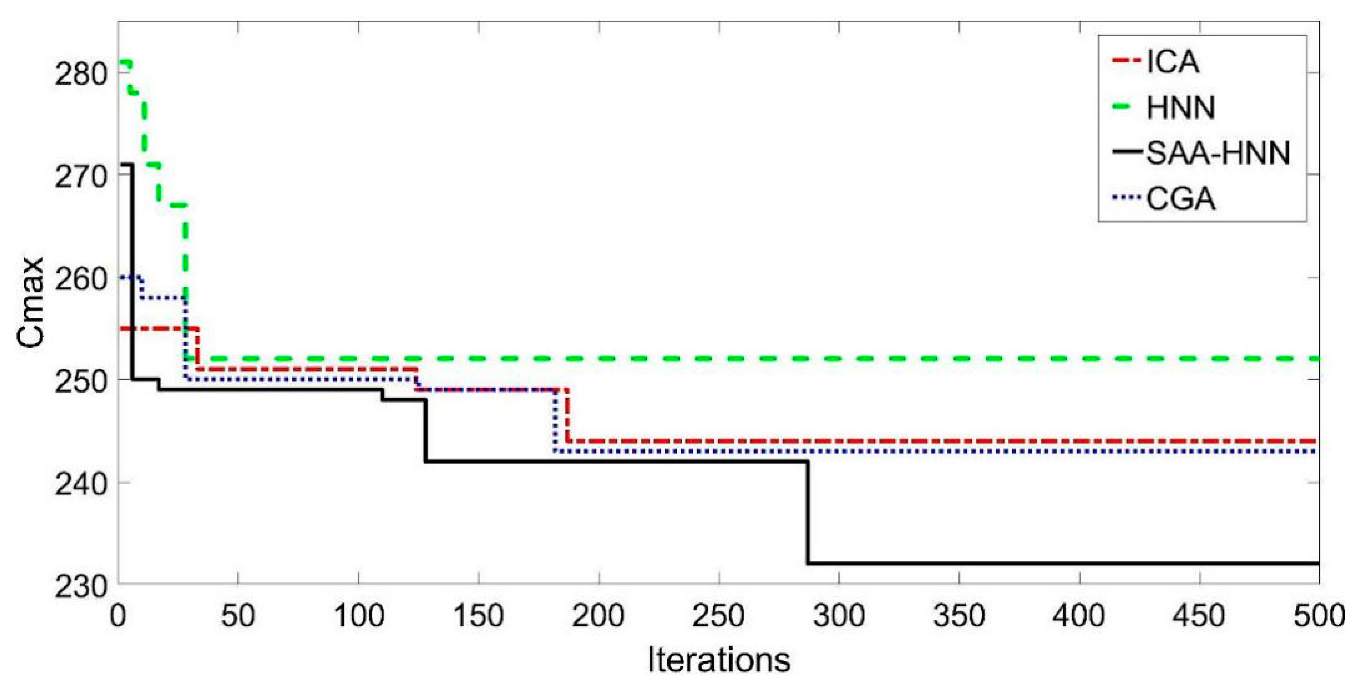
The correlation between the makespan $C_{max}$ and the iterations of four algorithms under actual production data are shown in Figure 5.

Figure 5 shows that the HNN algorithm converges rapidly in the initial stage of evolution but falls into local extremum prematurely due to the monotonous decrease in the energy function; it stagnates evolving in the 31st generation when $C_{max}$ converges to 252 eventually. The ICA and CGA algorithms have the ability of rapid optimization and convergence in the initial stage; however, they display integral convergence after evolving for a specific number of generations, making them easy to fall into local extremum. These phenomena stagnate evolving in the 221st and 185th generations, respectively, and their $C_{max}$ finally converge to 246 and 245, respectively. The SAA–HNN algorithm, which maintains the fast optimization feature of the HNN algorithm, converges rapidly in the initial stage of evolution, but falls into local extremum in the 127th generation. By introducing the idea of the simulated annealing algorithm, the ability of the SAA–HNN algorithm to jump out of local extremum is enhanced. Also, the SAA–HNN algorithm reactivates the evolutional process in the 278th generation, whose $C_{max}$ converges to 233 eventually.

From the above analysis of the scheduling evolutionary process, the SAA–HNN algorithm not only maintains the fast optimization characteristics of the HNN algorithm, but also jumps out of the local extremum and continues evolution in the process of solving the FFSP–PB problem with the improved local scheduling rules. Also, the SAA–HNN algorithm has better optimization effect than the ICA and CGA algorithms.

6. Conclusions

The present study investigated the FFSP–PB problem. Since the standard HNN algorithm easily falls into local extremum and is difficult for continuous evolution, this study proposed the SAA–HNN algorithm for global optimization. It adopts the Metropolis acceptance mechanism of the simulated annealing algorithm, such that the HNN algorithm can accept the non-optimal solution. Thus, the evolutionary vitality of the HNN algorithm is enhanced, rendering it the ability to jump out of the local extremum. Consecutively, considering the influence of the public buffer on the scheduling process, the reentrant rules of the electric flat carriage and workpiece transfer rules in the public buffer for controlling the movement of the workpiece are designed according to the transit time-cost of the workpiece among the workstation, the limited buffer, and the public buffer, as well as the processing status of the workpiece during the production. This phenomenon reduces the production blockage and improves the utilization of production resources. Finally, the simulation experiment proves that the SAA–HNN algorithm, combined with the improved local scheduling rules, can solve the FFSP–PB problem.

The actual production process has some local scheduling rules, such as setup time rules, process specification rules, and customer specification rules. If these local scheduling rules coexist with the relevant local scheduling rules established for the public buffer in the present study, the complexity of the whole scheduling optimization process would increase, and certain conflicts would occur between some of the local scheduling rules. Since the problem of conflict resolution between local scheduling rules are beyond the scope of this study, the main directions of future work are divided into the following:

(1)

Since the complex scheduling problem was investigated, the methods in the field of artificial intelligence should be explored to further improve the optimization effect and intellectualization of production scheduling algorithms.

(2)

Various local scheduling rules conflict with each other in the actual production system, necessitating that the method of effectively eliminating the conflicts between various local scheduling rules is explored further.

References

- Gao, Z.W.; Saxen, H.; Gao, C.H. Guest Editorial Special Section on Data-Driven Approaches for Complex Industrial Systems. IEEE Trans. Ind. Inform. 2013, 9, 2210–2212. [Google Scholar] [CrossRef]
- Gao, Z.W.; Kong, D.X.; Gao, C.H. Modeling and Control of Complex Dynamic Systems: Applied Mathematical Aspects. J. Appl. Math. 2012, 2012, 1–18. [Google Scholar] [CrossRef]
- Zambon, I.; Egidi, G.; Rinaldi, F. Applied Research Towards Industry 4.0: Opportunities for SMEs. Processes 2019, 7, 344. [Google Scholar] [CrossRef]
- Khamseh, A.; Jolai, F.; Babaei, M. Integrating sequence-dependent group scheduling problem and preventive maintenance in flexible flow shops. Int. J. Adv. Manuf. Technol. 2015, 77, 173–185. [Google Scholar] [CrossRef]
- Gerstl, E.; Mosheiov, G.; Sarig, A. Batch scheduling in a two-stage flexible flow shop problem. Found. Comput. Decis. Sci. 2014, 39, 3–16. [Google Scholar] [CrossRef]
- Gupta, J.N.D. Two-stage, Hybrid flow shop scheduling problem. Oper. Res. 1988, 39, 359–364. [Google Scholar] [CrossRef]
- Han, Z.H.; Ma, X.F.; Yao, L.L.; Shi, H.B. Cost Optimization Problem of Hybrid Flow-Shop Based on PSO Algorithm. Adv. Mater. Res. 2012, 532, 1616–1620. [Google Scholar] [CrossRef]
- Han, Z.H.; Sun, Y.; Ma, X.F.; Lv, Z. Hybrid flow shop scheduling with finite buffers. Int. J. Simul. Process Model. 2018, 13, 156–166. [Google Scholar] [CrossRef]
- Lalami, I.; Frein, Y.; Gayon, J.P. Production planning in automotive powertrain plants: A case study. Int. J. Prod. Res. 2017, 55, 5378–5393. [Google Scholar] [CrossRef]
- Han, Z.H.; Zhu, Y.H.; Ma, X.F.; Chen, Z.L. Multiple rules with game theoretic analysis for flexible flow shop scheduling problem with component altering times. Int. J. Model. Identif. Control 2016, 26, 1–18. [Google Scholar] [CrossRef]
- Nahas, N. Buffer allocation and preventive maintenance optimization in unreliable production lines. J. Intell. Manuf. 2017, 28, 85–93. [Google Scholar] [CrossRef]
- Hibino, H.; Yamamoto, M.; Yamaguchi, M.; Kobayashi, T. A study on Lot-Size dependence of energy consumption per unit of production throughput considering buffer capacity. Int. J. Autom. Technol. 2017, 11, 46–55. [Google Scholar] [CrossRef]
- Xi, S.H.; Chen, Q.X.; Mao, N.; Li, X.; Yu, A.L.; Zhang, H.Y. Capacity optimal configuration method of large-scale finite buffer production line. Comput. Integr. Manuf. Syst. 2017, 23, 2200–2210. [Google Scholar]
- Dolgui, A.B.; Eremeev, A.V.; Sigaev, V.S. Analysis of a multicriterial buffer capacity optimization problem for a production line. Autom. Remote Control 2017, 78, 1276–1289. [Google Scholar] [CrossRef]
- Gao, Z.W.; Nguang, S.K.; Kong, D.X. Advances in Modelling, Monitoring, and Control for Complex Industrial Systems. Complexity 2019. [Google Scholar] [CrossRef]
- Wang, X.H.; Gu, X.W.; Liu, Z.B. Production Process Optimization of Metal Mines Considering Economic Benefit and Resource Efficiency Using an NSGA-II Model. Processes 2018, 6, 228. [Google Scholar] [CrossRef]
- Georgiadis, G.P.; Elekidis, A.P.; Georgiadis, M.C. Optimization-Based Scheduling for the Process Industries: From Theory to Real-Life Industrial Applications. Processes 2019, 7, 438. [Google Scholar] [CrossRef]
- Han, Z.H.; Zhang, Q.; Shi, H.B. An Improved Compact Genetic Algorithm for Scheduling Problems in a Flexible Flow Shop with a Multi-Queue Buffer. Processes 2019, 7, 302. [Google Scholar] [CrossRef]
- Zhang, G.H.; Xing, K.Y. Differential evolution metaheuristics for distributed limited-buffer flowshop scheduling with makespan criterion. Comput. Oper. Res. 2019, 108, 33–43. [Google Scholar] [CrossRef]
- Rooeinfar, R.; Raissi, S.; Ghezavati, V.R. Stochastic flexible flow shop scheduling problem with limited buffers and fixed interval preventive maintenance: A hybrid approach of simulation and metaheuristic algorithms. Simulation 2019, 95, 509–528. [Google Scholar] [CrossRef]
- Jiang, S.L.; Zhang, L. Energy-Oriented Scheduling for Hybrid Flow Shop with Limited Buffers Through Efficient Multi-Objective Optimization. IEEE Access 2019, 7, 34477–34487. [Google Scholar] [CrossRef]
- Zeng, C.K.; Liu, S.X. Job Shop Scheduling Problem with Limited Output Buffer. Dongbei Daxue Xuebao J. Northeast. Univ. 2018, 39, 1679–1684. [Google Scholar] [CrossRef]
- Ribas, I.; Companys, R.; Tort-Martorell, X. An iterated greedy algorithm for solving the total tardiness parallel blocking flow shop scheduling problem. Expert Syst. Appl. 2019, 121, 347–361. [Google Scholar] [CrossRef]
- Chang, P.C. Reliability with finite buffer size for a multistate manufacturing system with parallel production lines. J. Chin. Inst. Eng. 2017, 40, 275–283. [Google Scholar] [CrossRef]
- Johri, P.K. A linear programming approach to capacity estimation of automated production lines with finite buffers. Int. J. Prod. Res. 1987, 25, 851–867. [Google Scholar] [CrossRef]
- Sun, S.Y.; Zheng, J.L. A modified algorithm and theoretical analysis for hopfield network solving TSP. Acta Electron. Sin. 1995, 23, 73–78. [Google Scholar]
- Yan, Y.L. A Solving Method to TSP Based on Improved Hopfield Neural Networks. J. Minnan Norm. Univ. 2014, 27, 37–43. [Google Scholar]
- Metropolis, N.; Rosenbluth, A.W.; Rosenbluth, M.N.; Teller, A.H.; Teller, E. Equation of state calculations by fast computing machines. J. Chem. Phys. 1953, 21, 1087–1092. [Google Scholar] [CrossRef]
- Neron, E.; Baptiste, P.; Gupta, J.N.D. Solving hybrid flow shop problem using energetic reasoning and global operations. Omega 2001, 29, 501–511. [Google Scholar] [CrossRef]
- Taillard, E. Benchmarks for basic scheduling problems. Eur. J. Oper. Res. 1993, 22, 278–285. [Google Scholar] [CrossRef]
- Carlier, J.; Neron, E. An exact met-hod for solving the multi-processor flow-shop. RAIRO Oper. Res. 2000, 34, 1–2. [Google Scholar] [CrossRef]
- Santos, D.L.; Hunsucker, J.L.; Deal, D.E. Global lower bounds for flow shop with multiple processors. Eur. J. Oper. Res. 1995, 80, 112–120. [Google Scholar] [CrossRef]
- Han, Z.H.; Dong, X.T.; Shi, H.B. Improved DE algorithm for hybrid flow shop load balancing scheduling problem. Comput. Integr. Manuf. Syst. 2016, 22, 548–557. [Google Scholar]
Figure 1.
Mathematical model of flexible flow shop with limited buffer and public buffer.
Figure 2.
The flowchart of the SAA–HNN algorithm.
Figure 3.
Box-plot of four algorithms for large-scale data j80c8a2.
Figure 4.
Gantt chart of scheme 3 scheduling result.
Figure 5.
Correlation between makespan and the iterations of four algorithms.