Article

Model Validation and Process Design of Continuous Single Pass Tangential Flow Filtration Focusing on Continuous Bioprocessing for High Protein Concentrations

by
Maximilian Johannes Huter
,
Christoph Jensch
and
Jochen Strube
*
Institute for Separation and Process Technology, Clausthal University of Technology, 38678 Clausthal-Zellerfeld, Germany
*
Author to whom correspondence should be addressed.
Submission received: 24 September 2019 / Revised: 22 October 2019 / Accepted: 23 October 2019 / Published: 1 November 2019
(This article belongs to the Section Biological Processes and Systems)

Abstract

:
In this study, the continuous Single-Pass Tangential Flow Filtration (SPTFF) concept is adapted for high protein concentrations. The work is based on the previously validated physico-chemical model for low concentrations and high viscosities. The model contains the Stagnant Film Model for concentration polarization, as well as the Boundary Layer Model for the mass transfer through the membrane. The pressure drop is calculated as a function of the Reynolds number. By performing preliminary experiments with a single ultrafiltration (UF) cassette, the model parameter are determined. The presented model is validated for a multi-step Single-Pass Tangential Flow Filtration. With subsequent simulation studies, an optimized process is found and confirmed by experiments. The outcome of this work shows the potential to optimize this multi-parameter dependent unit operation. This is reached by a model-based optimization allowing significant reduction of experimental efforts and applying the Quality by Design approach consistently. Furthermore, a comparison between the experimental setup and a commercial module is examined.

1. Introduction

In biopharmaceutical processes, membrane-based unit operations are chosen in several positions of the downstream processing (DSP). Due to their mild process conditions and low operation costs, they are used for different tasks in between the main purification steps. Next to sterile filtration, the protein concentration is enhanced by ultrafiltration and to exchange the surrounding medium diafiltration is used [1,2,3,4,5,6,7,8,9,10,11,12]. On the one hand, they are placed in front of the most purification steps to enhance their performance and lower production costs and on the other hand they are used in the end of the process for the formulation of the target protein [6]. The concentration of monoclonal antibodies for therapeutic use exceeds 150 g/L. These high concentrations of target molecules lead to increased viscosity and reaches values up to of 80 mPa·s [13]. This not only affects the pressure drop, but significantly lowers the filtration performance of the filtration setup and therefore boosts expenditure (OPEX). Even though solution adjustments of the pH value or by adding excipients are possible to lower the mentioned effects [14,15], a risk for precipitation remains with increasing salt concentrations [16]. Another approach to handle these highly concentrated solutions is by altering the filtration setup or geometries of the membrane cassettes.
Like in the previous study, this work focusses on modelling an SPTFF unit for ultrafiltration purposes [1]. Further information on the setup of continuous ultrafiltration and especially the multistep SPTFF is discussed in [1] as well. By implementing process models in the early stage of a process development, different combinations of unit operations can be evaluated. Next to the increased process development, process robustness and quality of the product are needed. Therefore, the Quality-by-Design (QbD) approach is demanded by authorities [17,18,19,20,21,22,23,24,
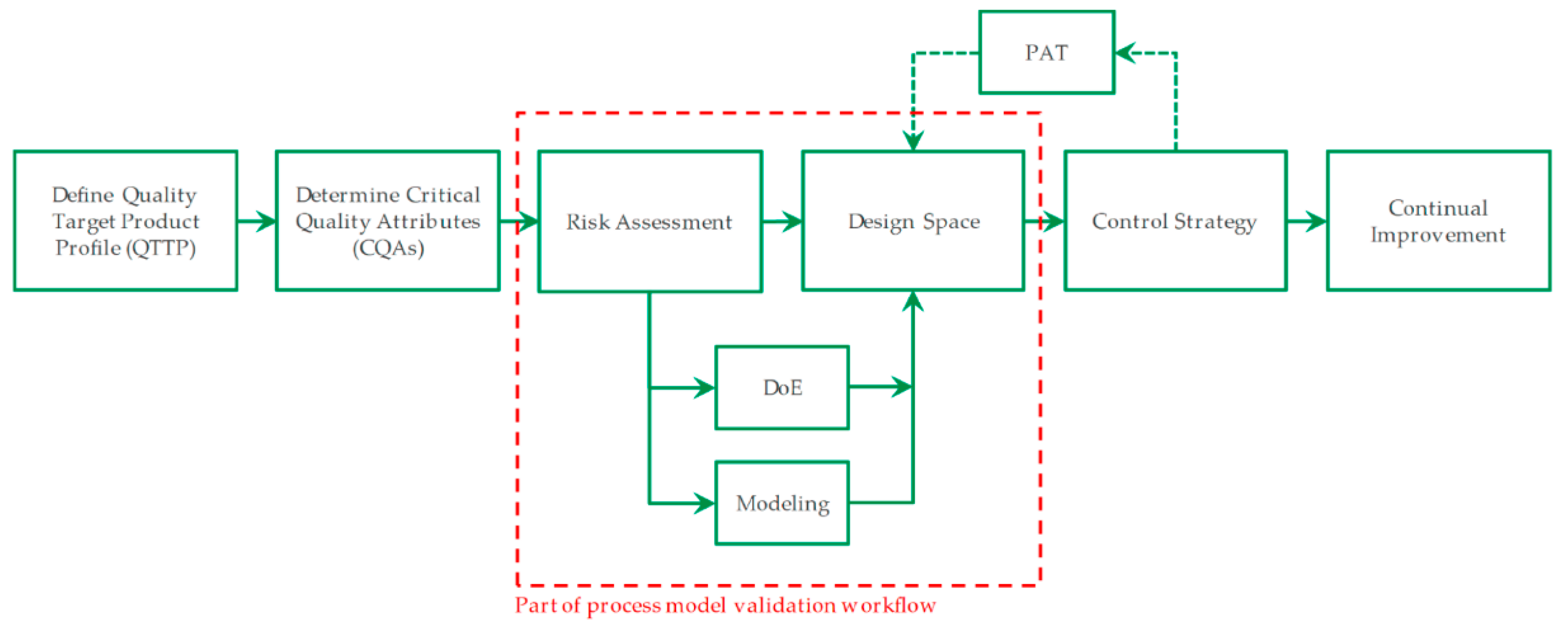
25]. An exemplary workflow for fast process development with usage of model-based process design is visualized in Figure 1. The red square marks the focused area, which is presented in this manuscript. To help evaluate the stability of each operation point inside the design space and sensitivities relating to operation parameters have to be identified. This leads to a more robust process. Because practical experiments would exceed a rational amount, model assisted process design is a promising approach.
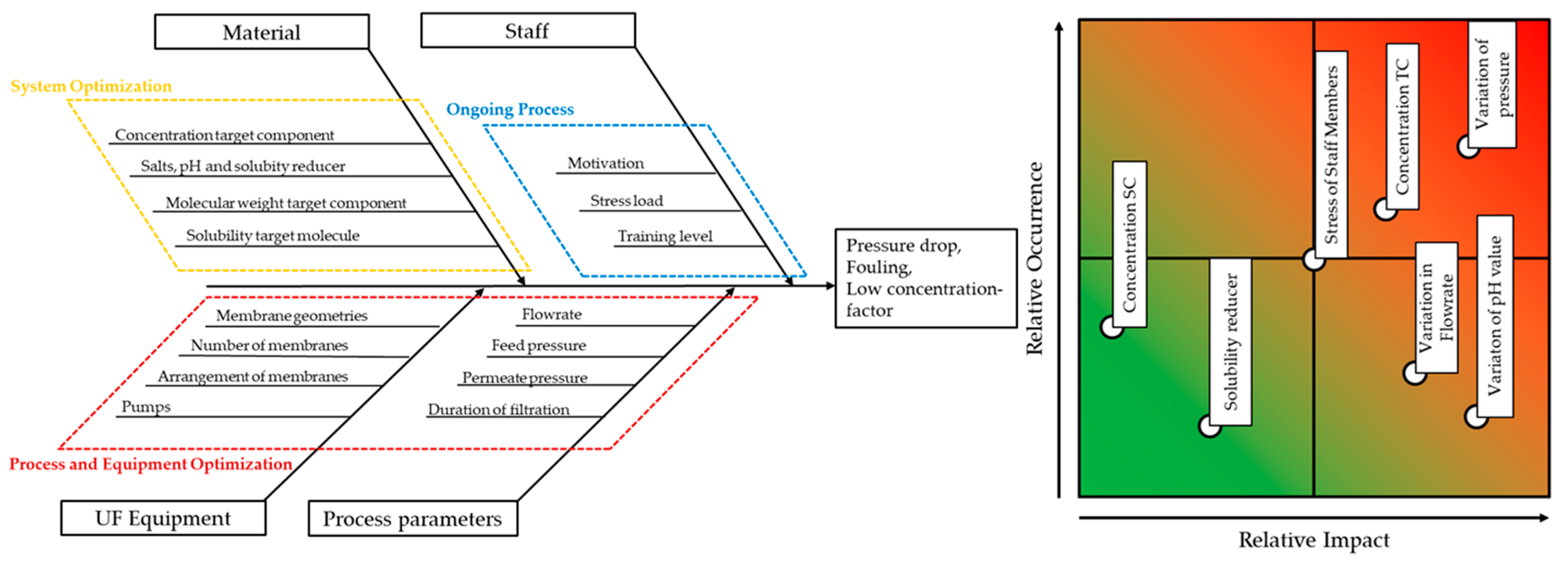
If model accuracy and precision are proven by few experiments, not only optimized assemblies can be developed, but also control strategies can be designed afterwards. For this purpose, the correlations must cover all possible parameters and ensure a stable process point. But at the first step, the critical quality attributes and product profiles have to be defined. Additionally, a risk assessment is required, which can be visualized with aid of Ishikawa diagrams and failure-mode-effect-analysis like shown in Figure 2. Even though this is not part of the model itself, it is part of the QbD approach. More on, this is helpful to define all necessary variables, which are relevant for position in the process.
While the Ishikawa (or Fish Bone) diagram is a qualitative approach to visualize the influences of the process, the Failure-Mode-Effect-Analysis (FMEA) is more quantitative and sorts relevant effects regarding its occurrence and its impact. In case of continuous ultrafiltration for proteins, the process is mainly influenced by pressure and flowrate. While higher flow rates increase the throughput, they also lead to higher feed pressures and pressure losses. Furthermore, the used equipment sets the boundaries for possible throughput and the used membrane configurations have an impact on the feed pressure resulting from the feed flow. Besides this process optimization, fluctuating pH values or other solubility reducers can affect the stability of the protein and lead to precipitation [
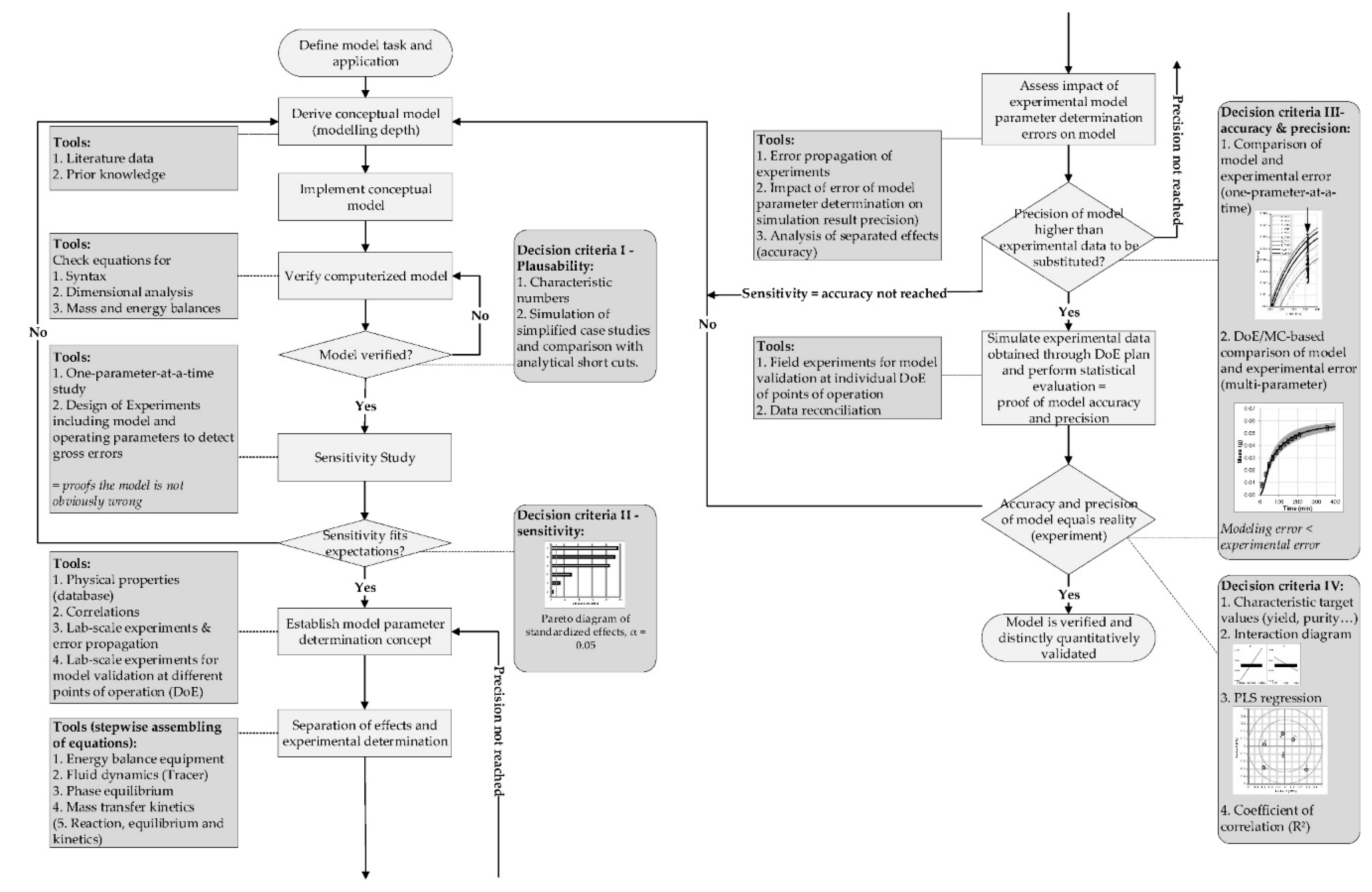
16]. This can result in fouling and reduction of filtration performance, but in a late stage of DSP, this is not likely to occur, which reduces the necessity for this aspect. The general workflow for model development is presented in Figure 3.
Step 1
At first, the design space has to be defined [26,27,28,29,30]. Like mentioned in Figure 2, ultrafiltration and specifically SPTFF is affected by several influences, like equipment (e.g., cassettes, setup), operating parameters (feed pressure, feed flow) and solution properties (concentration target component (TC), density, viscosity). This design space in return defines the necessary variables that the model must be able to reproduce (for example volumetric concentration factor (VCF) and pressure drop). In the sub sequential procedure, suitable equations have to be found from literature and prior knowledge to fulfill this task. Whether these equations lead to the correct results, can be checked with different approaches, like comparison of results to experimental or literature data. In case of this study, Step 1 is described in the previous study for protein concentrations below 5 g/L, but high viscosities up to 8 m Pas [1].
Step 2
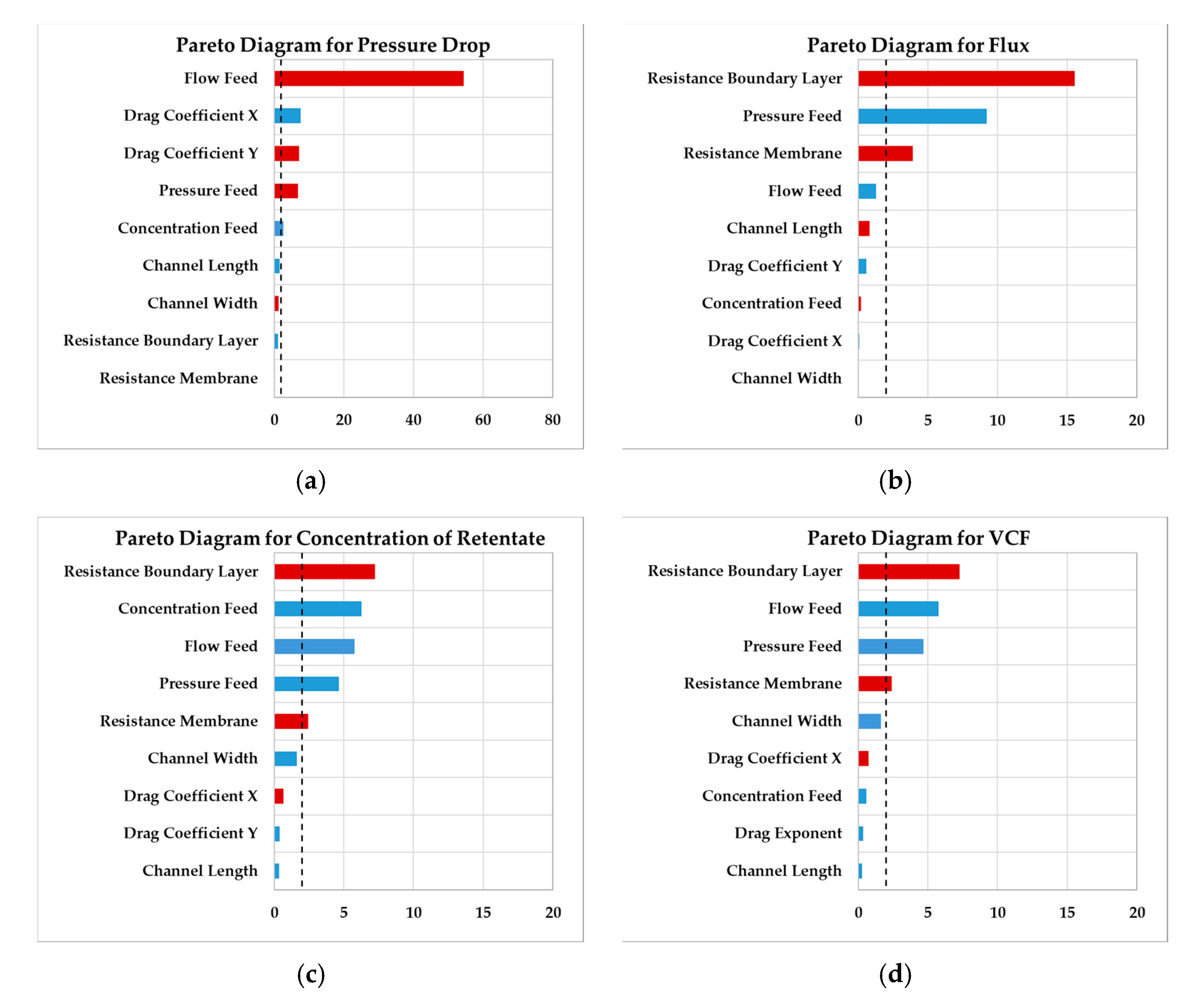
The second decision is based on sensitivity of process parameters. To develop a robust process, the sensitivity of each parameter affecting the unit operation has to be determined. By defining the possible range of the parameters, like design space of operating parameters or tolerances of the cassette, a model-based parameter study can be performed. Since the number of simulations is favorable reduced, statistical analyses of a design-of-experiments (DoE) plan are performed.
By feeding the simulation results into analysis tools, Pareto charts of standardized effects can be generated to visualize significance values. Using this analysis tools, it has to be kept in mind, that it is only valid for the given design space and is not applicable for further use without additional tests.
Step 3
Followed by the sensitivity study, the parameter determination concept is developed. Less significant parameters need a lower accuracy compared to sensitive parameters. The determination concept itself should separate effects so that the model itself becomes more modular. This modular approach allows a greater transferability to other systems. Geometrical properties should be measured first, solution properties in a sequential step [1].
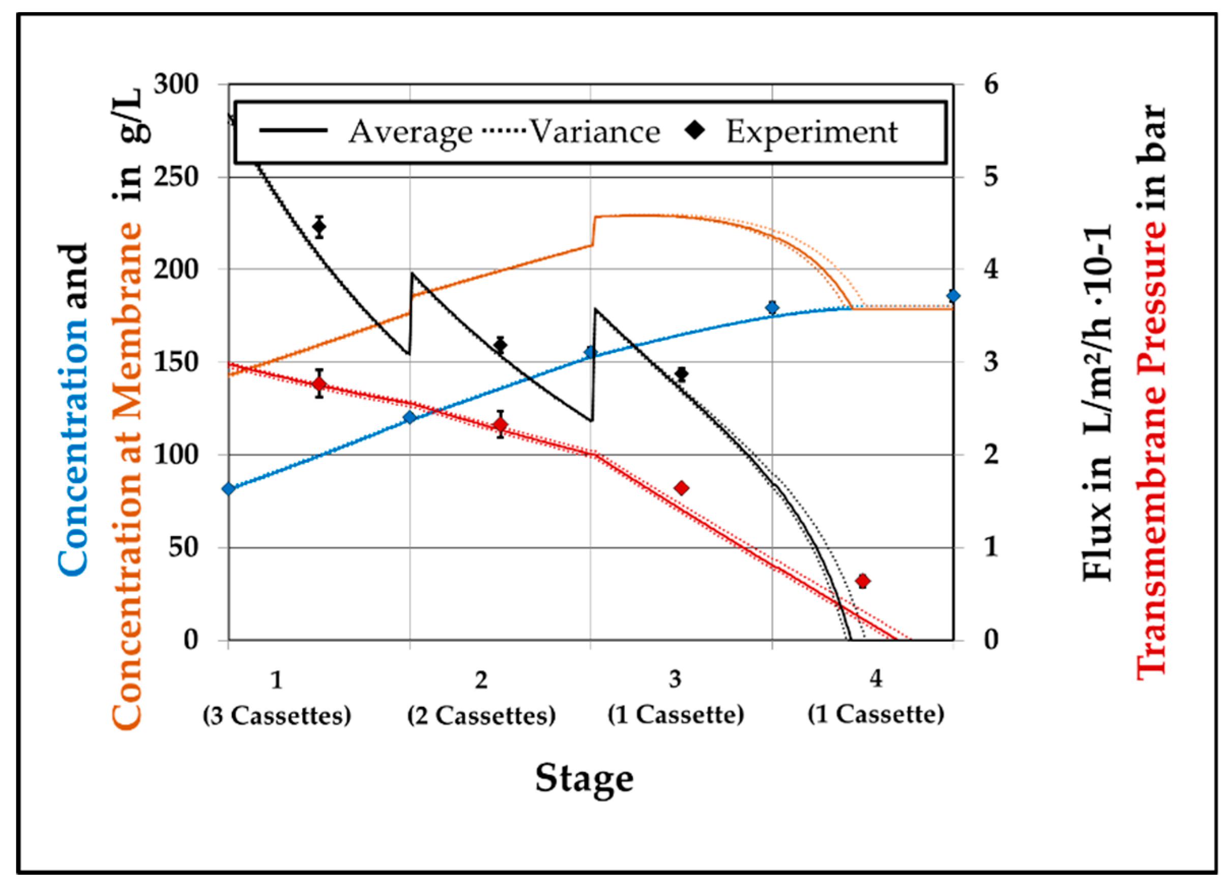
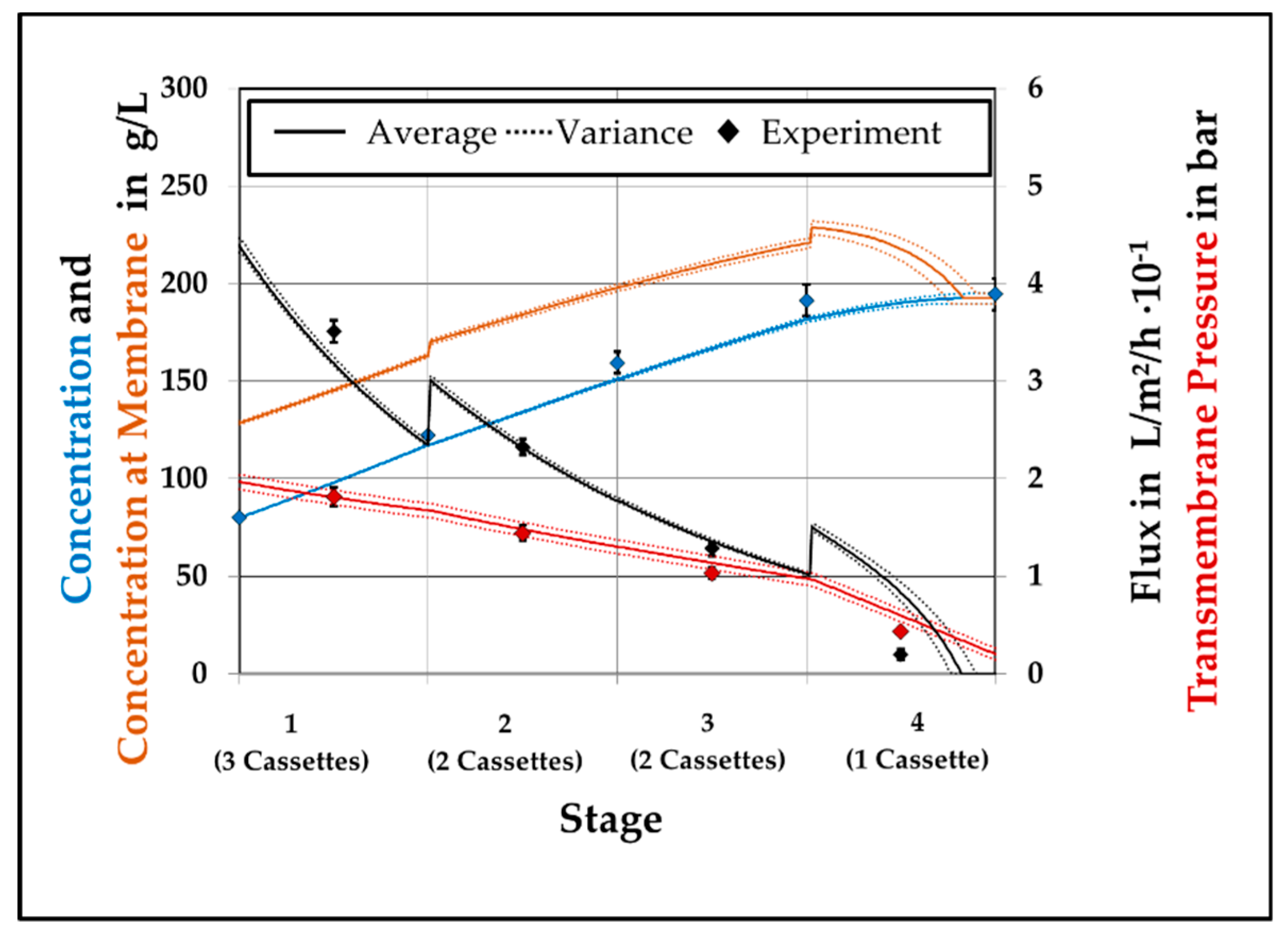
As a next step simulation and experimental results are compared for model validation. While this can be performed for each effect in a final attempt it has to be validated for the whole process step. In case of the researched multi-step SPTFF this also transfers the simulation from single cassettes to parallel and sequential structures. Due to this fact, small variations in the first stage can result in larger deviations in later stages, due to different ingoing parameters.
Step 4
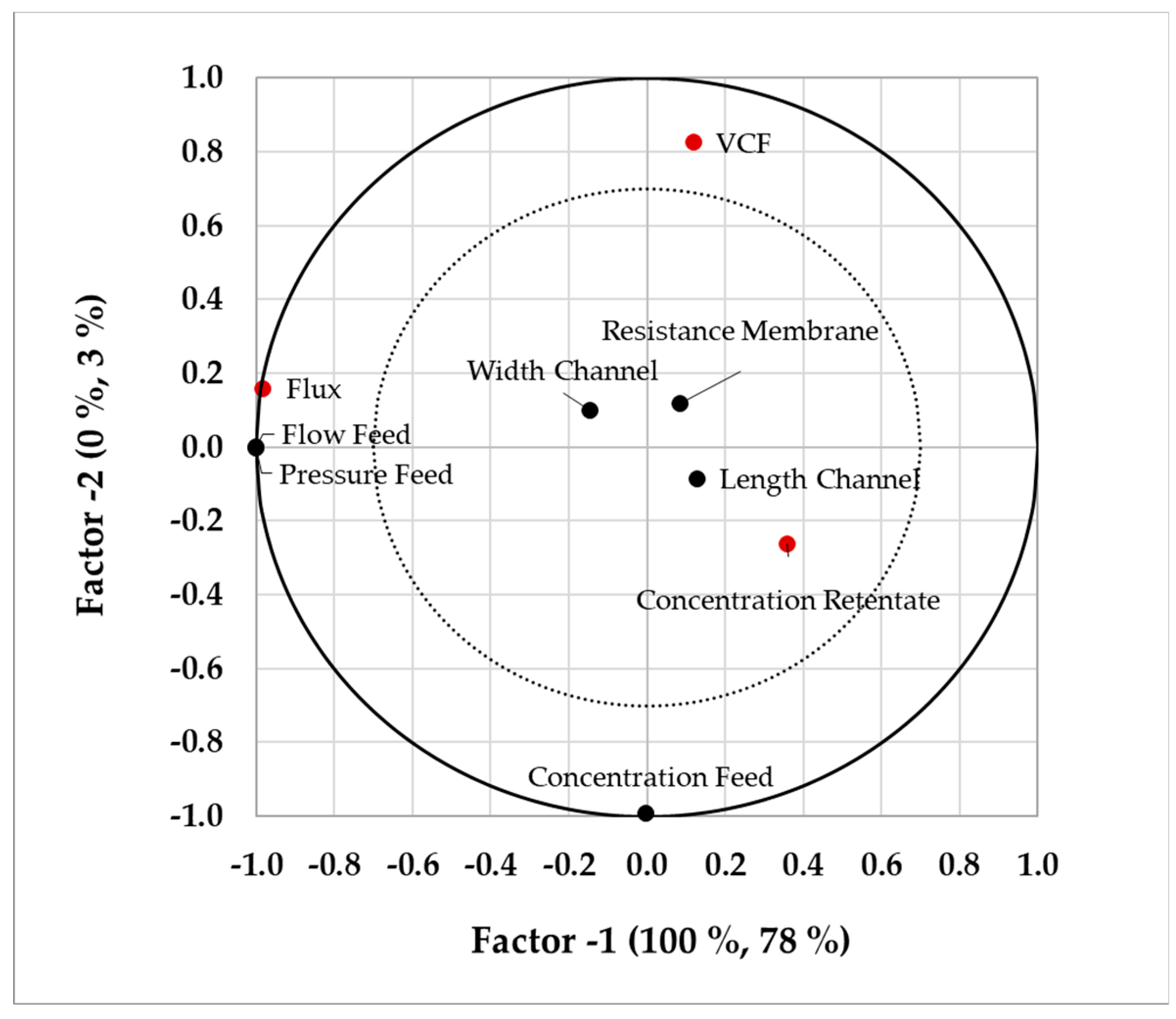
This last step is focused on the optimized operation point. For the performed simulation study, it has to be justified, that these studies are analyzed for the quality and performance attributes. In case of ultrafiltration, for example, concentration of the target protein and flux are target variables. This information, as well as the input parameters and boundaries, are fed into a statistical analysis tool. Partial least square (PLS) regression now helps to identify the correlations between input parameters and target values. Although PLS regression does not find causal relationships, it shows correlating effects. This helps to find critical process parameter and assesses the stability of the operation point.
With concluding these 4 steps, the model itself is verified and validated. Process development for the researched system, can be developed and optimized using the model. Model assisted process development was already performed for different unit operations: solid-liquid (phyto-) extraction [27], aqueous two-phase extraction of monoclonal antibodies [26], upstream fermentation of monoclonal antibodies [29] and chromatographic separation [30].
With this systematic approach, modelling can reduce experiments and accelerate the process design [28,31,32]. Furthermore, the optimal process parameters for a chosen design can be determined. The used model describes the mass transfer through the channel with a mass balance in which flux through the membrane results in lower velocity of the retentate stream. Furthermore, mass transfer through the membrane is described by using a Boundary Layer Model (BLM). With this model development of pressure, concentration, and flux can be visualized for the optical non-transparent device. With this visualization a process design of ultrafiltration modules becomes more reasonable and in a subsequent step the SPTFF module can be designed a priori. Additionally, the results of the experimental setup are compared to a commercial Cadence™ Single-Pass Tangential-Flow-Filtration Modular Kit.

2. Theory

2.1. Model Development

The presented model for SPTFF is based on earlier validated batch ultrafiltration models [7,8,9,10]. The model. It was transferred and enhanced for continuous ultrafiltration in the previous work [1].

2.1.1. Concentration Polarization

One of the major influences on tangential flow filtration is the concentration polarization. It reduces the flux and therefore lowers retentate concentrations. It can be calculated with the stagnant film model (SFM) developed by Michaels [33].
J v = k f · ln ( c M c B )
With Jv for the volumetric flux through the membrane, kf as mass transfer coefficient, cB is the concentration in the bulk phase and cM for the target component at the membrane wall. By changing the surrounding conditions like solution- or hydrodynamic influences this effect can be altered. For modelling a dynamic calculation of the mass transport coefficient is necessary. For this, the Sherwood correlation is used in this work.
Sh = k f l ch D p
The Sherwood number Sh is also derived from the following equations, consisting of the Schmidt number Equation (4) and the Reynolds number.
Sh = 1.664 + 0.33 Sc 0.33 Re 0.33
Sc = η Sol ρ Sol D P
Re = u eff l ch ρ Sol η Sol
The dynamic viscosity and molecular diffusion coefficient are calculated by the following correlations [8,13].
η Sol = 1 10 6 c B 3 3 10 4 c B 2 + 4.11 10 2 c B
D P = 8.314 · 10 8 [ cm · g 4 3 K · s 2 · mol 1 3 ] · T η Sol · M 1 3
The effective velocity is derived from Equation (8) [8]:
u eff = V ˙ A = V ˙ d h · w ch
With A as the cross-sectional area and V ˙ as the volume flow. The cross-sectional area is the product of the hydraulic diameter and the width of the membrane channel. In case of the used TFF cassettes, it is described by the hydraulic diameter and the width of the used screen [34,35]. For modelling, it assumed that effective velocity is reduced due to permeate flow, while the volume of solution in the membrane channel stays constant.

2.1.2. Boundary Layer Model

To describe the mass transport through the membrane the BLM is used. For this, on the one hand, the osmotic pressure difference has to be considered [3,8,11,33,36,37,38]. The difference of osmotic pressure lowers the driving force and results in a lowered mass transport through the membrane. For bovine serum albumin (BSA) the following equation describes the concentration depending.
P Osm = [ 3.7 · 10 1 · c M 2.98 · 10 3 · c M 2 + 1 · 10 5 · c M 3 ]
On the other hand, the intrinsic resistance of the membrane and the boundary layer resistance have to be determined. With the assumption of complete retention of the target molecule the flux is finally described by Equation (10) [1,39].
J v = TMP P Osm η p · ( R M + R BL )
where the transmembrane pressure is abbreviated TMP, POsm represents the osmotic pressure, ηp describes the dynamic viscosity of permeate, RM represents the membrane resistance, and RBL the boundary layer resistance.

2.1.3. Pressure Drop

The transmembrane pressure is not constant over the filtration path. The definition of the pressure loss at each point is described by the following term.
Δ p = p in p out
This pressure loss is influenced by the geometry of the membrane and the density of the solution. For modelling the drag coefficient cd membrane [33,34,36,40,41], with dh being the hydraulic diameter of the membrane.
Δ p = c d · ρ Solution u eff 2 · l ch 2 · d h
The drag coefficient cd is calculated from the plot over the Reynolds number Equation (13).
c d = X c · Re Y c
With Xc and Yc as experimental parameters, which must be determined for each cassette-type [41].

2.2. Influence of Protein Concentration

For filtration, the composition of the solution, especially the protein concentration, has major influences. While these influences have not been considered in the previous study [1], this work focusses on high protein concentrations. Figure 4 visualizes how the protein concentration affects osmotic pressure and dynamic viscosity of BSA [1,8]. In both cases, a high concentration leads to major reduction of filtration performance. While the osmotic pressure decreases with the salt concentration of the buffer system, like Binabaji et al. presented for a monoclonal antibody [14], it has to be considered for low salt solutions.
With the curve in Figure 4 it gets obvious that after a concentration of around 80 g/L both, osmotic pressure and dynamic viscosity, have a significant effect, which accelerates with increasing protein concentration. For formulation purposes, it has to be shown that the filtration step is also predictable and may be optimized with model calculations.

3. Material & Methods

3.1. Filtration Setup

For experimental work 30 kDa T01 cassettes (Pall, Waltham, MA, USA) with an area of 100 cm2 per cassette and a screen channel were used. Each single membrane and membrane stacks were inserted into membrane holders, with 1/8″ in and outlets. In addition to the stage-separated setup, the results were compared to a Cadence™ SPTFF Modular Kit (Pall, Waltham, MA, USA). For pumping a Quattroflow QF 150 (Almatec, Duisburg, Germany) was used. For both setups 1/8″ tubing was used.

3.2. Media

Each experiment was performed with 5 L of an 80 g/L BSA solution. The value 80 g/L was chosen, assuming the given setup reaches a VCF of at around 2 and therefore a final concentration of 150 g/L is achievable. The protein was dissolved in a 10 mM KPi buffer at a pH value of 7. For clean water resistance tests (CWRT), purified water was acquired with the Sartorius arium® 157 pro (Sartorius®, Gottingen, Germany).

3.3. Analytics

For inline measurements of the divided setup five pressure transmitters AP016 (Autosen, Essen, Germany) were used. In case of the modular kit two of the same kind were applied. The weight development of feed, retentate and all permeate streams were measured with PCE-TB 6 scales (PCE Deutschland GmbH, Meschede, Germany).

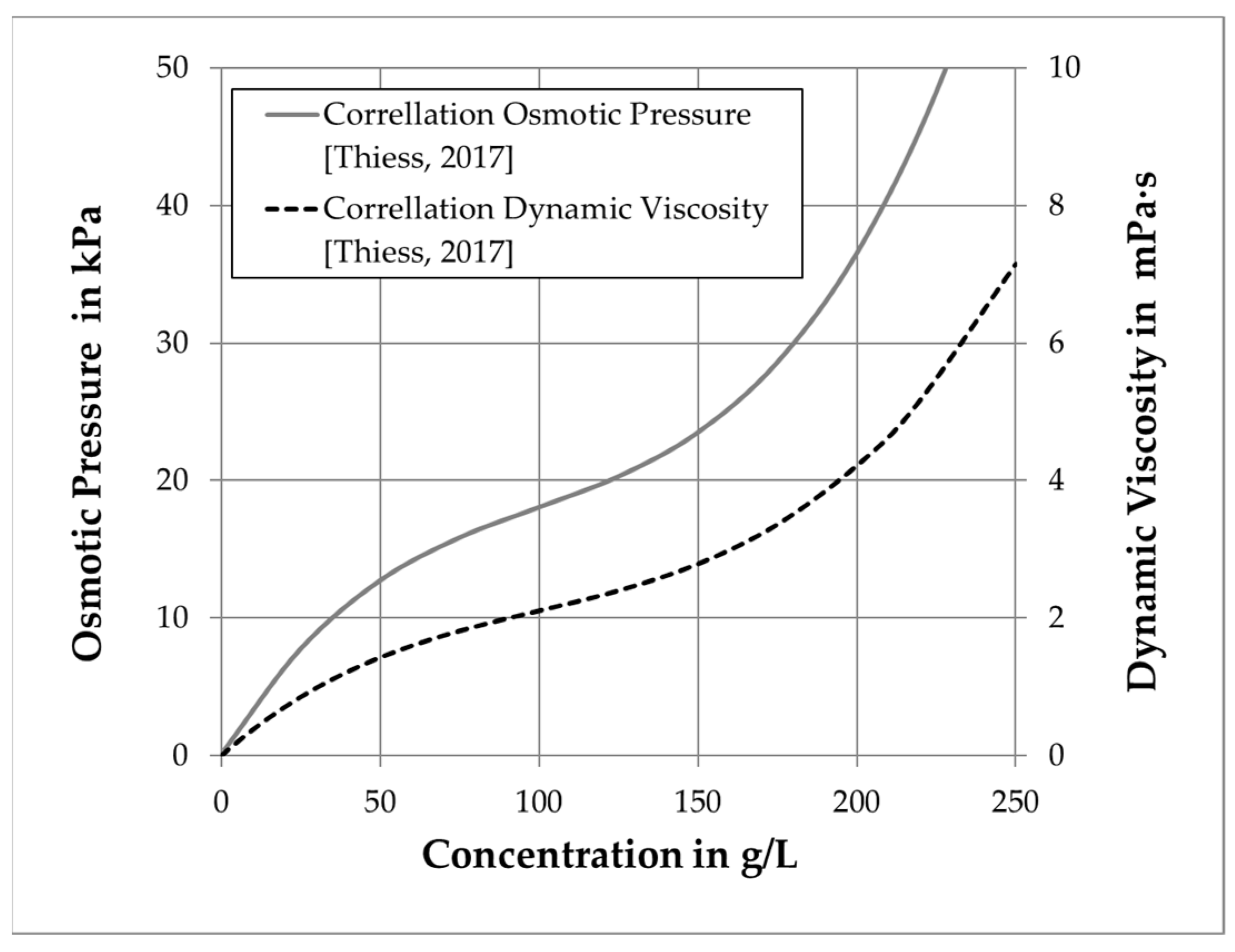
3.4. Dataset for Modelling

All module related parameters, like geometries, resistances, and drag factors were measured experimentally. Solution properties of the BSA were based on the correlations from [8].
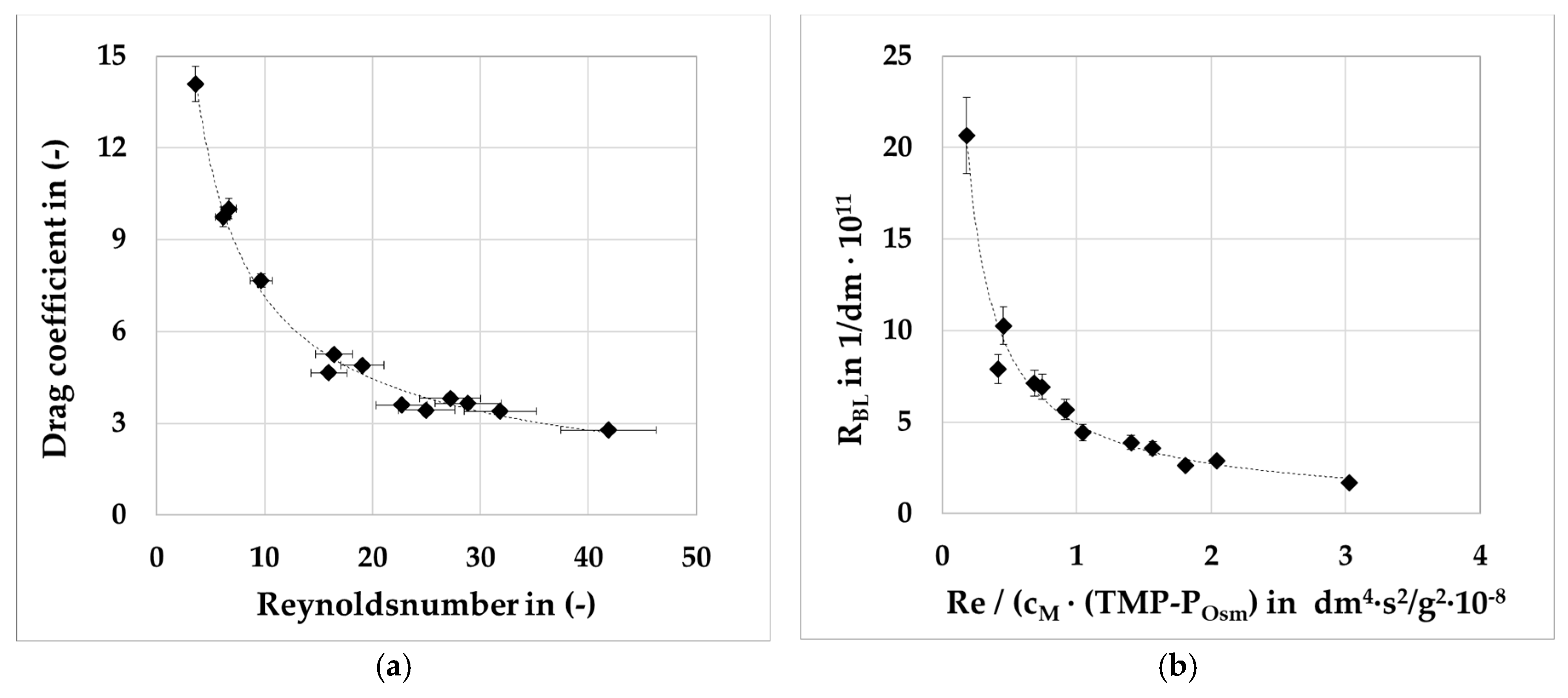
At first, a single cassette had to be measured regarding its geometrical data (Area, hydraulic diameter). Furthermore, its intrinsic membrane resistance (RMem) and drag coefficient (cd) were determined via clean water resistance tests (CWRTs) [1]. In the following step the 80 g/L BSA solution were filtrated at several transmembrane pressures and flowrates using retentate valves. With information of these experiments RBL can be determined. The model was built in Aspen Custom Modeler™ (Aspen Tech, Bedford, MA, USA), statistical analysis was performed with JMP (SAS Institute, Cary, NC, USA) and the PLS with Unscrambler® X (Camo Analytics, Oslo, Norway).

3.5. Design of Experiments

Ultrafiltration setups, like the SPTFF, have several process parameters. On the one hand, there are the geometrical properties (area per cassette, screen geometries) predetermined by the supplier and chosen setup and on the other hand, there are feed flow, feed pressure and temperature. While the type of the cassettes was not varied during this study, the setup of the SPTFF is changeable. Due to temperature sensitivity of the target protein, it is not rational to alter the temperature. In addition, in a laboratory setup feed flow and feed pressure affect each other, which reduces the process parameter to one active parameter. In case of this work feed pressure was chosen. The upper limit was 4 bar, given by the supplier. The lower limit on the other hand, is based on a minimal throughput of around 50 mL/min for the commercial 4-in-series module of Pall and equals 2 bar. For validation of the SPTFF filtration model the center point was performed three times under the same conditions. Each experiment had a duration of 60 min and samples were taken from the retentate in 5 min steps. After each experiment the membranes were cleaned with 0.2 M NaOH and stored in 0.1 M NaOH.

4. Results and Discussion

4.1. Sensitivity Study

With the generated model a sensitivity study of several parameters is examined. This is performed to investigate the influences of several process parameters on the process itself. In this case, only one cassette is considered. The different variables and ranges are described in Table 1.
The results for this sensitivity study for the process variables pressure drop, flux, concentration of retentate, and volumetric concentration factor (VCF), which describes the ration between final and inital concentration, are shown in Figure 5a–d. In these charts red marked Influences had a negative t-ratio, while blue ones had a positive one. For the analysis 67 simulations have been performed including a 3 time repetition of the center point. The simulations proved to be sufficient for a p-value lower than 0.0001 for simulation vs. prediction response.
As we can see in Figure 5b–d, the RBL is the most sensitive parameter. In addition, the feed flow has a great sensitivity especially for the pressure drop of the system. While the drag coefficients of a cassette had no sensitive effect on cRet, flux and VCF of a single cassette, it is sensitive for the pressure drop of the system. More on, it would affect a multistep filtration for the other variables as well because the pressure loss would result in a reduced feed pressure for the sequential cassette. Since pressure loss, flux, cRet and retentate concentration affect each other, it should be noted that none of the considered parameters can be neglected. Especially the feed flow and the boundary layer resistance have to be emphasized as extremely sensitive factors which have a vital influence on the ultrafiltration step.

4.2. Parameter Determination

Like those presented in the previous manuscript [1] and mentioned above, membranes are characterized as the first step. These geometry depending parameters are displayed in Table 2. The generated curve to determine the drag factor coefficients is shown in Figure 6a.
The second step is to determine the influences on RBL with a single cassette. In Figure 6b the resistance is plotted to all the influences evident from the experiments. These are the concentration of the protein at the membrane, the flow regime represented by the Reynolds number and the main driving force which is the TMP lowered by the osmotic pressure.
At low flowrates the resistance increases drastically, while higher flowrates lead to a strongly reduced value. In addition, higher concentrations and high transmembrane pressures raise the resistance and therefore reduce the filtration capability of cassettes. The performed experiments lead to the following correlation:
R Bl = X R · ( Re c M · ( TMP P Osm ) ) Y R
With the values 8694 g 2 · s 2 dm 5 for XR and −0.84 for YR at a R² of 0.97.

4.3. Model Validation

For validation of the model, the 4-in series setup by Pall is used, like in the previous work [1]. It consists of a 3-2-1-1 structure, where stage 1 and 2 have parallel structures (3 cassettes in stage 1, 2 cassettes in stage 2). The comparison between experiment and model is visualized in Figure 7 and the resulting process variables shown in Table 3. In this figure, the horizontal axis represents the length of pathway from inlet of stage 1 to outlet of the final stage. It is sectioned in stages, where each stage equals the length of one cassette. In case of the T01 a stage corresponds to 14.1 cm. The figure contains the values for concentration (blue) of the target component. Since measurements inside the cassette are not possible, the concentration is measured by analyzing permeate and retentate flows. The concentration at the membrane (orange) is not measurable and therefore cannot be compared with experiments. In contradiction to the concentration, flux (black) and transmembrane pressure (red) are presented as the average over the membrane cassette. The feed flow was 67 mL/min at a pressure of 3 bar.
The predicted process variables of the simulation match the experimental data with only a difference of 5.2% in VCF. It is detectable, that the model slightly underestimates the flux, resulting in an increased retentate flow. Due to the higher velocity, the pressure drop is increased compared to the experiments. But keeping the different sensitivities in mind, it is obvious that the presented model is capable to predict the experimental data with a high accuracy, by knowing feed flow and feed pressure. Based on these results, it is possible to perform model-based optimization studies.

4.4. Model Assited Optimization

In this chapter, the model is used to perform the setup and operation parameter study. Because feed pressure and feed flow are, only one operational parameter is active and for this study, the feed pressure was chosen. The feed flow for each setup was estimated by the results from parameter determination. It is assumed, that each stage has a VCF of 1.3 which is the average factor of each stage in the validation (chapter 4.2) experiment and the overall pressure drop of all stages leads to the feed pressure of stage 1. The simulated results of feed pressure variation for different setups are depicted in Figure 8a–d and it is an adaption from the optimization procedure shown in [42]. The different setups consist of 6 to 8 cassettes, to have just a little variation to the standard setup. In addition, a subsequent stage does not contain more cassettes than the preceding stage.
Figure 8a visualizes that for all setups an increase of pressure does not lead to an improved filtration performance. In each considered case the VCF is lowered, when the pressure is raised. In addition, the VCF is also reduced with increased permeate flux. This is because feed flux and permeate flux have a nearly linear dependency where the gradient of each filtration setup is greater than 1. The mass throughput per feed flux gradient equals for all setups. From the graphs above, it gets obvious that the 3-2-2-1 setup has the best results regarding VCF, followed by the 3-3-1-1 in lower pressure regions and the 2-2-2-2 for pressures greater 2.5 bar. Figure 8d shows that the gradient of feed flux per permeate flux is lower for the setups, which generate the highest VCF.
Based on this study the 3-2-2-1 setup is chosen as configuration. Its optimal point process parameter is the lowest feed pressure, which in this case is 2 bar. As the final step of this study, simulated optimized setup and experimental values are compared in Figure 9 and Table 4. While the study uses predicted values for feed flow, the comparison between model and optimized experiment used the feed flow from the experiment. For 2 bar feed pressure the flow is 51.8 mL/min.
Like in the validation experiment of the center point, visualized in Figure 3, the simulated values match the experimental values with no difference at the end of the process. Again the flux of the first stage is slightly underestimated. For the following stages, the flux is consistent with the experiments, but the pressure loss is lower. This leads to a significant higher flux in the last stage, but all in all the same final concentration is reached. The pressure drop in the model in contradiction is lower compared to the experiments. It is obvious that the model is capable to predict the experimental data with high accuracy.
The last step is to identify the correlations between the input parameters and the resulting process variables. By performing Monte Carlo simulations for the process parameters and evaluating them statistically with partial least square (PLS) regression a correlation loading plot is created and shown in Figure 10. The black points are the predictors and represent the input parameters and the resulting variables are marked red. By extracting the “principal components” from input parameters and target variables via PLS regression, the maximum of covariance between predictor and responses is explained. Even though two factors are often not enough to explain 100% of the variance, the correlation loadings plot only consists of two factors, which have the main influence. For further clarification, two circles are inserted. The dotted circle represents the limit for 50% explained variance and the other one the 100% explained variance.
As we can see the flux mainly correlates with factor 1 (significant distance to the 0.0 value of Factor 1), while the VCF is dominated by factor 2. While the flux positively correlates with feed flow and feed pressure (nearly the same position on the visualized plot), which means a high pressure or flow results in increased flux, VCF and final concentration negatively correlates with these two parameters. An increased flux does not necessarily lead to high concentrations, because the retentate flow rises as well and perhaps even stronger than the flux (see Figure 8a–d). While the retentate concentration increases at high feed concentrations, the VCF is lowered. This is because an increased feed concentration reduces filtration performance, but also has an increased starting point probably leading to higher concentrations. All parameters around the center, which in this case are the tolerances of geometrical dimensions and the intrinsic membrane resistance, are less important, which agrees with the sensitivity study in chapter 4.1.

4.5. Comparison to Commercial SPTFF-Kit

In Addition, the experiments above were performed with a Cadence™ Single-Pass TFF Modular Kit. For this, the same cassettes are used and stacked into a single membrane unit. In this case, no pressure detectors are set in between the stages and the separation and junction of the different retentate streams are performed by special gaskets. For the modular kit, the feed flow leads to a higher feed pressure resulting in the assumption that the outlet of the retentate is smaller than 1/8”. At 3 bars the feed flow equals 57 mL/min and for 2 bar it reduces to 49 mL/min. The comparison between model and performed experiments is shown in Table 5.
Like in the previous tests with separated stages, the model is capable to predict the VCF with a difference lower than 5%. In both cases the model has slightly better results than the experiments themselves. For obvious reasons the pressure drop shows a much higher difference up to 10%, because the retentate valve is not implemented in the model. More on, just a minor improvement due to lowering of the TMP and insertion of an additional cassette is detectable. These experiments contradict the assumption, that retentate valves have no significant effect [12]. While this effect probably lowers with number of stages, in case of the researched 4-stage setup the valve has a significant influence. However, it should be noted that the model can also be used for the kit, but feed flow and feed pressure must be known for this.

5. Conclusions

This study for modelling a continuous ultrafiltration step showed the possibility to develop a versatile process design and optimization tool for high concentrated protein solutions. By separating the general model into different sub models and divide the membrane model into geometry depending and solution depending properties, accurate predictive simulations can be performed. Like in the previous study [
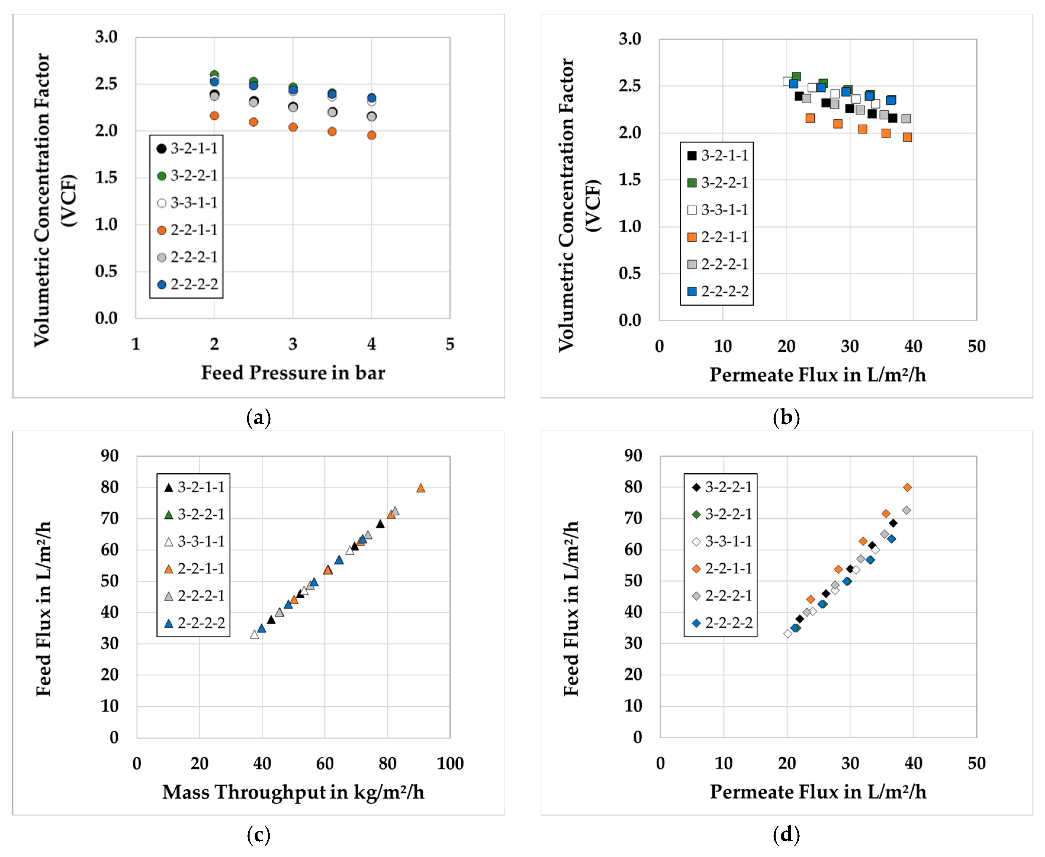
1] accurate predictions for the VCF are reached with less than 5% divergence to experimental values. It has been shown that for a system without a retentate valve the performance can be increased by adding a second membrane to stage 3 and reducing the feed pressure to 2 bar. In case of the Cadence® SPTFF Kit a fixed reduction of the cross-sectional area in the end of the module makes an insertion of an additional membrane negligible. As it gets obvious that the TMP should be as low as possible, from a production point of view a compromise between throughput and VCF has to be found. By performing the PLS regression the dependencies are presented and the model is verified.
In order to transfer this approach to diafiltration, the parameter and dependencies for solution-based properties have to be investigated. On the one hand, the development of density and viscosity with concentration can variate and on the other hand RBL and POsm can be altered, too.
As it is presented in this study, it is possible to predict filtration behavior of a complex setup based on single cassette performances with a small amount of experiments. Furthermore, all necessary experiments can be performed with a single cassette and are transferable to complex setups. This enables a process design a priori and reduces possible experimental effort, if the configuration of different stages is changeable.

Author Contributions

M.J.H. performed experiments, developed the model, did the simulations as well as wrote this paper. C.J. performed experiments and reviewed this paper. J.S. is responsible for conception and supervision.

Funding

The authors want to thank the Bundesministerium für Wirtschaft und Energie (BMWi), especially M. Gahr (Projektträger FZ Jülich), for funding this scientific work.

Acknowledgments

We gratefully acknowledge the support of G. Kalinowski (Pall Corporation) for kindly providing the filtration cassettes and the Cadence™ Single-Pass TFF Modular Kit. Additionally, we want to thank the ITVP lab-team especially Frank Steinhäuser and Volker Strohmeyer for their effort and support.

Conflicts of Interest

The authors declare no conflict of interest.

Symbols and Abbreviations

AFactor for osmotic Pressure
BLMBoundary layer model
BSABovine serum albumin
CConcentration in the liquid phase, g/L
cMConcentration at membrane, g/L
cBConcentration in bulk phase, g/L
cFConcentration of feed, g/L
cRetConcentration of retentate, g/L
CWRTClean water resistance test
dhHydraulic diameter, m
DoEDesign of experiments
DpMolecular diffusion coefficient, m²/s
DSPDownstream processing
FMEAFailure Modes and Effect Analysis
JvVolumetric flux, L/m²/h
kfMass transfer coefficient, m/s
LchLength of channel, m
OPEXOperational expenditure
PPressure, bar
PATProcess analytical technology
PLSPartial least square
pOSMOsmotic pressure, bar
QbDQuality by design
RMResistance of Membrane, 1/m
RBLResistance of Boundary layer, 1/m
ScSchmidt number, -
SCSide component
ShSherwood number
SFMStagnant film model
TTemperature, °C
TCTarget component
TMPTransmembrane pressure, bar
ueffEffective velocity, m/s
VVolume, dm³
wchWidth of channel, m
VCFVolumetric concentration factor, -
XcFactor for drag coefficient, -
XRFactor for boundary layer resistance, g²·s²/dm5
YcExponent for drag coefficient, -
YRExponent for boundary layer resistance, -
ρSoldensity of solution, g/L
ηSoldynamic viscosity of solution, g/m/s
ηpdynamic viscosity of permeate, g/m/s

References

  1. Huter, M.J.; Strube, J. Model-Based Design and Process Optimization of Continuous Single Pass Tangential Flow Filtration Focusing on Continuous Bioprocessing. Processes 2019, 7, 317. [Google Scholar] [CrossRef]
  2. Cheryan, M. Ultrafiltration and Microfiltration Handbook; Technomic Pub. Co.: Lancaster, PA, USA, 1998. [Google Scholar]
  3. Baker, R.W. Membrane Technology and Applications, 3rd ed.; Wiley: Chichester, UK, 2012. [Google Scholar]
  4. Jungbauer, A. Continuous downstream processing of biopharmaceuticals. Trends Biotechnol. 2013, 31, 479–492. [Google Scholar] [CrossRef] [PubMed]
  5. Zydney, A.L. Continuous downstream processing for high value biological products: A Review. Biotechnol. Bioeng. 2016, 113, 465–475. [Google Scholar] [CrossRef] [PubMed]
  6. Sommerfeld, S.; Strube, J. Challenges in biotechnology production—Generic processes and process optimization for monoclonal antibodies. Chem. Eng. Process.: Process Intensif. 2005, 44, 1123–1137. [Google Scholar] [CrossRef]
  7. Fröhlich, H.; Villian, L.; Melzner, D.; Strube, J. Membrane Technology in Bioprocess Science. Chem. Ing. Tech. 2012, 84, 905–917. [Google Scholar] [CrossRef]
  8. Thiess, H.; Leuthold, M.; Grummert, U.; Strube, J. Module design for ultrafiltration in biotechnology: Hydraulic analysis and statistical modeling. J. Membr. Sci. 2017, 540, 440–453. [Google Scholar] [CrossRef]
  9. Grote, F.; Fröhlich, H.; Strube, J. Integration of Reverse-Osmosis Unit Operations in Biotechnology Process Design. Chem. Eng. Technol. 2012, 35, 191–197. [Google Scholar] [CrossRef]
  10. Grote, F.; Fröhlich, H.; Strube, J. Integration of Ultrafiltration Unit Operations in Biotechnology Process Design. Chem. Eng. Technol. 2011, 34, 673–687. [Google Scholar] [CrossRef]
  11. Charcosset, C. Membrane Processes in Biotechnology and Pharmaceutics; Elsevier Verlag: Oxford, UK, 2012. [Google Scholar]
  12. Dizon-Maspat, J.; Bourret, J.; D’Agostini, A.; Li, F. Single pass tangential flow filtration to debottleneck downstream processing for therapeutic antibody production. Biotechnol. Bioeng. 2012, 109, 962–970. [Google Scholar] [CrossRef]
  13. Binabaji, E.; Ma, J.; Zydney, A.L. Intermolecular Interactions and the Viscosity of Highly Concentrated Monoclonal Antibody Solutions. Pharm. Res. 2015, 32, 3102–3109. [Google Scholar] [CrossRef]
  14. Binabaji, E.; Ma, J.; Rao, S.; Zydney, A.L. Ultrafiltration of highly concentrated antibody solutions: Experiments and modeling for the effects of module and buffer conditions. Biotechnol. Prog. 2016, 32, 692–701. [Google Scholar] [CrossRef] [PubMed]
  15. Lutz, H.; Arias, J.; Zou, Y. High concentration biotherapeutic formulation and ultrafiltration: Part 1 pressure limits. Biotechnol. Prog. 2017, 33, 113–124. [Google Scholar] [CrossRef] [PubMed]
  16. Scopes, R.K. Protein Purification. Principles and Practice, 3rd ed.; Springer-Verlag: Berlin/Heidelberg, Germany, 1994. [Google Scholar]
  17. ICH. Quality Risk Management Q9, (Step 4 version); ICH: Geneva, Switzerland, 2005; Available online: https://www.ich.org/fileadmin/Public_Web_Site/ICH_Products/Guidelines/Quality/Q9/Step4/Q9_Guideline.pdf (accessed on 17 January 2018).
  18. ICH. Pharmaceutical Quality System Q10, (Step 4 version); ICH: Geneva, Switzerland, 2008; Available online: http://www.ich.org/fileadmin/Public_Web_Site/ICH_Products/Guidelines/Quality/Q10/Step4/Q10_Guideline.pdf (accessed on 17 January 2018).
  19. ICH. Pharmaceutical Development Q8 (R2), (Step 4 version); ICH: Geneva, Switzerland, 2009; Available online: https://www.ich.org/fileadmin/Public_Web_Site/ICH_Products/Guidelines/Quality/Q8_R1/Step4/Q8_R2_Guideline.pdf (accessed on 2 January 2015).
  20. ICH. Development and Manufacturing of Drug Substances Q11, (Step 4 version); ICH: Geneva, Switzerland, 2013; Available online: http://www.ich.org/fileadmin/Public_Web_Site/ICH_Products/Guidelines/Quality/Q11/Q11_Step_4.pdf (accessed on 17 January 2018).
  21. Degerman, M.; Westerberg, K.; Nilsson, B. A Model-Based Approach to Determine the Design Space of Preparative Chromatography. Chem. Eng. Technol. 2009, 32, 1195–1202. [Google Scholar] [CrossRef]
  22. Del Val, I.J.; Kontoravdi, C.; Nagy, J.M. Towards the implementation of quality by design to the production of therapeutic monoclonal antibodies with desired glycosylation patterns. Biotechnol. Prog. 2010, 26, 1505–1527. [Google Scholar] [CrossRef]
  23. FDA. Guidance for Industry: Pharmacogenomic Data Submissions. Biotechnol. Law Rep. 2003, 23, 68–86. [Google Scholar]
  24. US Department of Health and Human Services. Guidance for Industry—Sterile Drug Products Produced by Aseptic Processing—Current Good Manufacturing Practice; FDA: Silver Spring, MD, USA, 2004.
  25. Food and Drug Administration. Guidance for Industry PAT—A Framework for Innovative Pharmaceutical Development, Manufacturing, and Quality Assurance; FDA: Silver Spring, MD, USA, 2004.
  26. Schmidt, A.; Strube, J. Distinct and Quantitative Validation Method for Predictive Process Modeling with Examples of Liquid-Liquid Extraction Processes of Complex Feed Mixtures. Processes 2019, 7, 298. [Google Scholar] [CrossRef]
  27. Sixt, M.; Uhlenbrock, L.; Strube, J. Toward a Distinct and Quantitative Validation Method for Predictive Process Modelling—On the Example of Solid-Liquid Extraction Processes of Complex Plant Extracts. Processes 2018, 6, 66. [Google Scholar] [CrossRef]
  28. Sixt, M.; Strube, J. Systematic and Model-Assisted Evaluation of Solvent Based- or Pressurized Hot Water Extraction for the Extraction of Artemisinin from Artemisia annua L. Processes 2017, 5, 86. [Google Scholar] [CrossRef]
  29. Kornecki, M.; Strube, J. Accelerating Biologics Manufacturing by Upstream Process Modelling. Processes 2019, 7, 166. [Google Scholar] [CrossRef]
  30. Zobel-Roos, S.; Mouellef, M.; Ditz, R.; Strube, J. Distinct and Quantitative Validation Method for Predictive Process Modelling in Preparative Chromatography of Synthetic and Bio-Based Feed Mixtures Following a Quality-by-Design (QbD) Approach. Processes 2019, 7, 580. [Google Scholar] [CrossRef]
  31. Sixt, M.; Strube, J. Systematic Design and Evaluation of an Extraction Process for Traditionally Used Herbal Medicine on the Example of Hawthorn (Crataegus monogyna JACQ.). Processes 2018, 6, 73. [Google Scholar] [CrossRef]
  32. Zobel-Roos, S.; Schmidt, A.; Mestmäcker, F.; Mouellef, M.; Huter, M.; Uhlenbrock, L.; Kornecki, M.; Lohmann, L.; Ditz, R.; Strube, J. Accelerating Biologics Manufacturing by Modeling or: Is Approval under the QbD and PAT Approaches Demanded by Authorities Acceptable Without a Digital-Twin? Processes 2019, 7, 94. [Google Scholar] [CrossRef]
  33. Michaels, A.S. New Separation Technique for CPI. Chem. Eng. Prog. 1968, 64, 31–43. [Google Scholar]
  34. Da Costa, A.R.; Fane, A.G.; Fell, C.J.D.; Franken, A.C.M. Optimal channel spacer design for ultrafiltration. J. Membr. Sci. 1991, 62, 275–291. [Google Scholar] [CrossRef]
  35. Saeed, A. Effect of Feed Channel Spacer Geometry on Hydrodynamics and Mass Transport in Membrane Modules. Ph.D. Thesis, Curtin University, Perth, WA, Australia, 2012. [Google Scholar]
  36. Wijmans, J.G.; Nakao, S.; Smolders, C.A. Flux limitation in ultrafiltration: Osmotic Pressure Model and Gel Layer Model. J. Membr. Sci. 1984, 20, 115–124. [Google Scholar] [CrossRef]
  37. Binabaji, E.; Rao, S.; Zydney, A.L. The osmotic pressure of highly concentrated monoclonal antibody solutions: Effect of solution conditions. Biotechnol. Bioeng. 2014, 111, 529–536. [Google Scholar] [CrossRef]
  38. Yousef, M.A.; Datta, R.; Rodgers, V.G.J. Free-Solvent Model of Osmotic Pressure Revisited: Application to Concentrated IgG Solution under Physiological Conditions. J. Colloid Interface Sci. 1998, 197, 108–118. [Google Scholar] [CrossRef]
  39. Wijmans, J.G.; Nakao, S.; van den Berg, J.W.A.; Troelstra, F.R.; Smolders, C.A. Hydrodynamic resistance of concentration polarization boundary layers in ultrafiltration. J. Membr. Sci. 1985, 22, 117–135. [Google Scholar] [CrossRef] [Green Version]
  40. Young, M.E.; Carroad, P.A.; Bell, R.L. Estimation of diffusion coefficients of proteins. Biotechnol. Bioeng. 1980, 22, 947–955. [Google Scholar] [CrossRef]
  41. Da Costa, A.R.; Fane, A.G.; Wiley, D.E. Spacer characterization and pressure drop modelling in spacer-filled channels for ultrafiltration. J. Membr. Sci. 1994, 87, 79–98. [Google Scholar] [CrossRef]
  42. Pall Life Sciences. Application Note—Volume Reduction and Process Optimization with Cadence™ Inline Concentrator; Pall Life Sciences: PALL: Nassau County, NY, USA, 2013. [Google Scholar]
Figure 1. Workflow chart for process design with process modelling as its central part [26]. Reproduced with permission from A. Schmidt, Processes; published by MDPI, 2019. (With process analytical technology abbreviated PAT and DoE standing for design of experiments.).
Processes 07 00781 g001
Figure 2. Quality-by-Design (QbD) assessment for ultrafiltration (UF) and diafiltration: Ishikawa diagram and Failure-Mode-Effect-Analysis (FMEA).
Processes 07 00781 g002
Figure 3. Workflow for Process- and model development [26]. Reproduced with permission from A. Schmidt, Processes; published by MDPI, 2019.
Processes 07 00781 g003
Figure 4. Dependency of osmotic pressure and dynamic viscosity of bovine serum albumin (BSA) concentration.
Processes 07 00781 g004
Figure 5. Sensitivity study—Pareto diagrams for (a) pressure drop (b) flux (c) concentration of retentate (d) volumetric concentration factor (VCF)—positive t-ratios are marked blue and negative ones are marked red.
Processes 07 00781 g005
Figure 6. Parameter determination curves for (a) drag factor coefficients with R2 0.98 and (b) boundary layer resistance with R2 0.97.
Processes 07 00781 g006
Figure 7. Axial profiles of concentration(blue), concentration at the membrane (orange), flux (black) and transmembrane pressure (red) for experiments and model prediction of BSA filtration.
Processes 07 00781 g007
Figure 8. Simulated values for different setups (a) Volumetric concentration factor vs. feed pressure (b) Volumetric concentration factor vs. permeate flux (c) Feed flux vs. Mass throughput (d) feed flux vs. permeate flux.
Processes 07 00781 g008
Figure 9. Axial profiles of concentration (blue), concentration at the membrane (orange), flux (black) and transmembrane pressure (red) for experiment and model prediction of the optimized process.
Processes 07 00781 g009
Figure 10. Correlation loadings plot visualizing the dependencies of the variables based on Monte Carlo simulations.
Processes 07 00781 g010
Table 1. Sensitivity study: Feed parameter and expected effect for pressure drop and volumetric concentration factor (VCF) for a single cassette in Single-Pass Tangential Flow Filtration (SPTFF).
VariableRangeUnitExplanationExpected Effect
Pressure dropVCF
Feed concentration75–85(g/L)80 g/L represents the medium concentration, with 5 g/L variation to represent process fluctuations of prior separation units.LowMedium
Feed flow17–45(mL/min)With 50 mL/min as minimal throughput for the stacked system, 17 mL represents the lower boundary for a single cassette. With the used pump the maximal feed flow was 45 mL per channel, until 4 bar feed pressure are reached.HighHigh
Feed pressure2.0–4.0(bar)2 bar represent the minimal pressure which is reached at 50 mL/min for a stacked system. 4 bar is the maximum operation pressure, described by the manufacturer.HighHigh
Membrane length1.39–1.43(dm)For length and width of the membrane a tolerance of ± 2 mm is assumedLowNo
Membrane width0.34–0.38(dm)MediumLow
Drag factor Xc30–35(-)For both drag factor coefficients, the variation of the drag coefficients of the previous study are takenMediumLow
Drag factor Yc−0.75–−0.80(-)MediumLow
RM2.5–4.0(1/m) × 1012For membrane resistance the range of typical values for 30 kDa membranes are taken.LowMedium
RBL1–20(1/m) × 1012The boundary layer resistance showed a broad variation in prior experiments. To represent this, a large range is assumedMediumHigh
Table 2. Module parameter.
ParameterUnitValue
Effective membrane area per cassette(m²)0.01
Hydraulic diameter(m)1.01 × 10⁻⁴
Drag factor coefficients
Xc(-)36.8
Yc(-)−0.68
RM(1/m) × 10123.25 ± 0.4
Table 3. Comparison of experimental and simulated process variables.
VCF (-)Pressure Drop (bar)
Experiment2.31 ± 0.122.92 ± 0.01
Model prediction2.19 ± 0.123.00 ± 0.00
Difference5.2%2.8%
Table 4. Comparison of experimental and simulated process variables for the optimized process.
VCF (-)Pressure Drop (bar)
Experiment2.44 ± 0.071.94 ± 0.08
Model prediction2.44 ± 0.031.79 ± 0.02
Difference0%8%
Table 5. Comparison of experimental and simulated process variables for SPTFF kit.
Validation ExperimentOptimized Process
VCF [-]Pressure Drop [bar]VCF [-]Pressure Drop [bar]
Experiment2.37 ± 0.022.84 ± 0.12.41 ± 0.051.98 ± 0.01
Model prediction2.46 ± 0.052.66 ± 0.12.48 ± 0.021.69 ± 0.02
Difference4.7%6.4%3.1%10%

