Splitting Triglycerides with a Counter-Current Liquid–Liquid Spray Column: Modeling, Global Sensitivity Analysis, Parameter Estimation and Optimization

Abstract

In this work we present the model of a counter-current spray column in which a triglyceride (tripalmitic triglyceride) is hydrolyzed by water and leads to fatty acid (palmitic acid) and glycerol. A finite volume model (FVM) of the column was developed to describe the reactive extraction process with a two-phase system and validated with an analytical model from the literature with the given data set encompassing six experimental runs. Global, variance-based (Sobol) sensitivity analysis allowed assessment of the sensitivity of the sweet water glycerol content in respect to liquid density, overall mass-transfer coefficient, reaction rate coefficient and the equilibrium ratio to rank them accordingly. Furthermore, parameter estimation with a differential evolution (DE) algorithm was performed to obtain among others the mass transfer, backmixing and reaction rate coefficients. The model was used to formulate and solve a process design problem regarding economic and sustainable performance. Multi-criteria optimization was applied via DE to minimize total annual cost (TAC) and the Eco99 indicator by varying the steam inlet flow rate and distribution over the two steam inlets as the independent variables. The model and analysis was implemented in Fortran and Python where the Fortran model can also be embedded in a process simulator such as PRO/II or Aspen.

1. Introduction

Vegetable oils are mixtures of triglycerides of different composition subject to the type and origin of the oil. The derived intermediates from vegetable oils are glycerol, methyl esters, fatty acids and fatty alcohols and can be regarded as the platform chemicals in the oleochemical domain. Triglycerides have side chains with even C-numbers in natural oils and thus fatty acids processed from vegetable oils are also composed of even C-chains. The global vegetable oil market has grown to a worldwide market and is expected to reach 30 billion US Dollars in the year of 2024 of which the Southeast Asian (Asian-Pacific) region holds the largest market share. With the highest proportion, fatty acids made up 55% of the total demand in 2015 [1]. Applications of oleochemicals range from food and cleaning to beauty products. This makes vegetable oil a suitable substitute for petroleum-based products; however, it is critically discussed if and how bio fuels (fatty acid methyl esters, in short FAME) should be produced from this source via transesterification [2,3,4]. In this work we will discuss hydrolysis as the chemical conversion route of triglycerides which takes place in the industrial applied spray column unit operation.

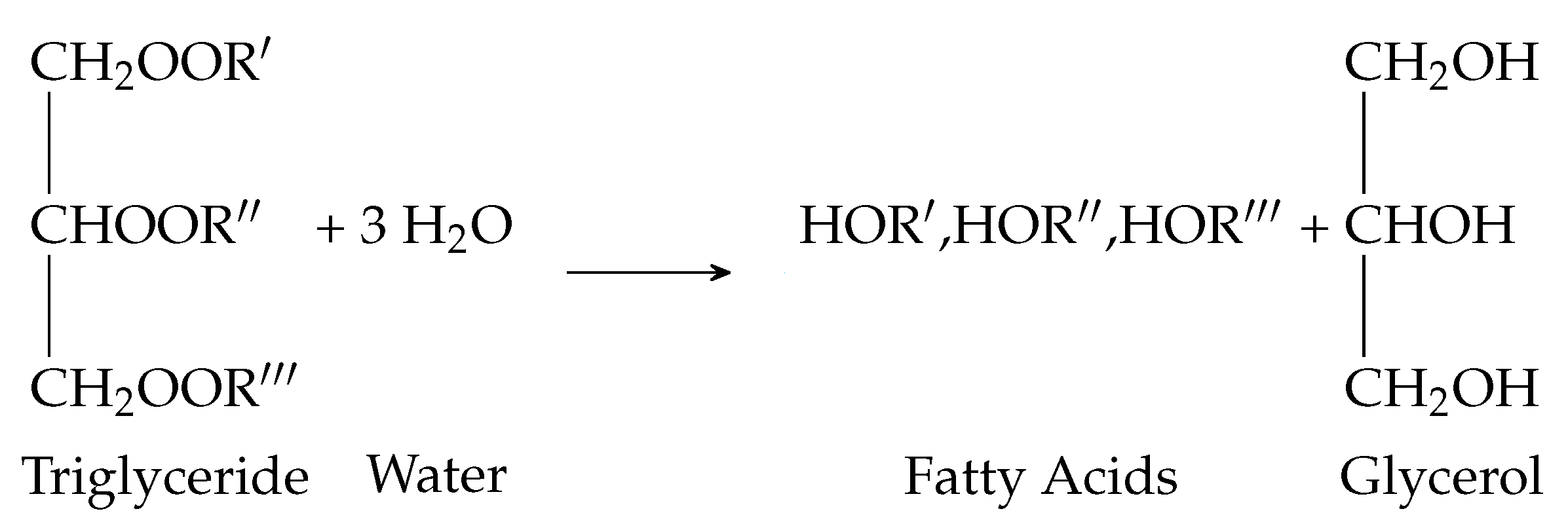
1.1. Hydrolysis Reaction

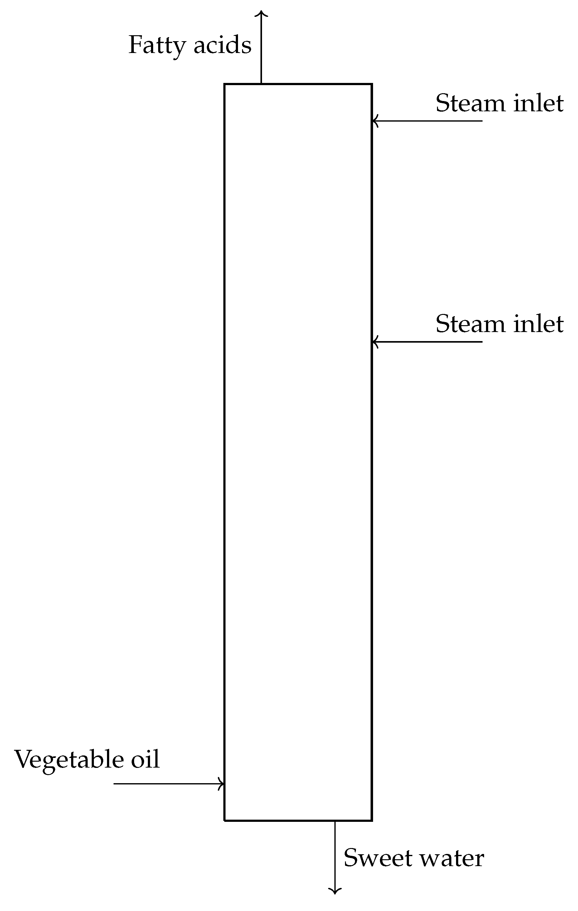
The hydrolysis of triglycerides is the reaction to perform if fatty acids or glycerol are the desired products. Figure 1 shows the general hydrolysis scheme of triglycerides where the fatty acid sidechains depicted with the letter R can vary in length and saturation (amount of double bonds).

Studies on the hydrolysis of fats and oils have been performed over several decades and are summarized in

Table 1. Studies in the literature on the hydrolysis of fats and oils.

First Author	Reactor Type	Reaction Type and Order	Catalyst and Process Conditions	Model and Studied Parameters
Patil [5]	CSTR	Reversible & Pseudo-1st Order	None	Algebraic Equations
Forero-Hernandez [6]	Batch		None
Lascaray, 1949 [7]	Review	Review	Review; 100–220 ${}^{°}$C	-
Lascaray, 1952 [8]	Review	Review	Review; 100–220 ${}^{°}$C	-
Sturzenegger and Sturm [9]	Batch	Irreversible & Pseudo-1st Order	ZnO
Jeffreys [10]	Spray column	Irreversible & Pseudo-1st Order	ZnO	Algebraic Equations
Rifai [11]	Spray Column	Reversible & 2nd Order?
Namdev [12]	Review	Reversible & Pseudo-1st Order
Attarakih [13]	Spray column	Reversible & Pseudo-1st Order		Reduced Population Balance Model

. The hydrolysis reaction is discussed in this section and the research on counter-current spray columns is elaborated subsequently.

Patil et al. [5] investigated the hydrolysis reaction in a continuous-stirred tank reactor and proposed a three-step reversible reaction scheme for the hydrolysis of tri- (TG), di- (DG) and monoglycerides (MG) with water (W) to give fatty acids (FA) and glycerol (GLY) where DG and MG act as intermediates:

$$\mathrm{T}\mathrm{G}+\mathrm{W}\underset{-k_1}{\overset{k_1}{\rightleftharpoons }}\mathrm{D}\mathrm{G}+\mathrm{F}\mathrm{A}$$

$$\mathrm{D}\mathrm{G}+\mathrm{W}\underset{-k_2}{\overset{k_2}{\rightleftharpoons }}\mathrm{M}\mathrm{G}+\mathrm{F}\mathrm{A}$$

$$\mathrm{M}\mathrm{G}+\mathrm{W}\underset{-k_3}{\overset{k_3}{\rightleftharpoons }}\mathrm{G}+\mathrm{F}\mathrm{A}$$

These three reactions can be aggregated into a single step reaction where the triglycerides react with water to fatty acids and glycerol:

$$\mathrm{T}\mathrm{G}+3\mathrm{W}\underset{-k}{\overset{k}{\rightleftharpoons }}3\mathrm{F}\mathrm{A}+\mathrm{G}$$

Forero-Hernandez et al. [6] show with the experimental data set from Alenezi et al. [14] that the identified mass-transfer coefficient and reaction rate constants are highly correlated. The experimental data are based on the non-catalyzed hydrolysis of sunflower oil in a batch autoclave at 300 ${}^{°}$C.

A three reaction regime over time is assumed based on the work by Patil et al. [15] and Aniya et al. [16], where the first heterogeneous regime in the interface is mass-transfer controlled, the second pseudo-homogeneous regime in the oil phase is controlled by the irreversible fast chemical reaction, and the third homogeneous regime in the oil phase is reaching the reversible chemical equilibrium reaction controlled state (Figure 2).

1.2. Spray Column

The result of an extensive literature search led to the identification of one data set which could be used for validating the finite volume model of a counter-current spray column (Figure 3) developed in this work. This data set was found in the work of Jeffreys et al. and their work is outlined in the following section with an additional section depicting contributions by Rifai et al. [11].

1.2.1. Research by Jeffreys et al.

The analytical model calculations by Jeffreys et al. [10] rely on reaction rate data by Sturzenegger and Sturm [9] (catalyst level of 0.25% zinc oxide) and the value of 0.17 1/min was used as the reaction rate constant. The reaction is assumed to be of pseudo-first order and irreversible. It is assumed that the water content in the continuous phase is in excess and constant. Jeffreys et al. imply (referencing Mills and McClair [17]) that the increase of the continuous phase and the decrease with respectively 4% and 7% of the dispersed aqueous mass flow rate is negligible. As a consequence of this assumption the solubility of water in the oil phase will be about 10% at process conditions. The continuous and dispersed phase mass flows are being assumed constant regardless of the internal column position and the dispersed phase droplets are assumed to travel through the column at the same velocity. In the discussion of their results Jeffreys et al. state that in the lower part of column the chemical reaction is the bottleneck to the mass-transfer-controlled process. Furthermore, they mention the unfavorably operation at 18% flooding capacity which should rather be 30–40% as suggested by Minard and Johnson [18] to amend the mass-transfer process. Jeffreys et al. present an analytic algebraic equation for the glycerol fraction in the aqueous phase over the height of the column. The overall mass-transfer coefficient $Ka$ is obtained for six experimental data sets from a laboratory scale spray column. The work by Jeffreys et al. is also used as the reference to validate and discuss other developed models in the publications by Rifai et al. [11], Namdev et al. [12] and Attarakih et al. [13].

1.2.2. Research by Rifai et al.

Rifai et al. [11] proposed a modified version of the linear, steady-state spray column model established by Jeffreys et al. They present a non-linear model with the water solubility in the continuous phase being a function of composition and the variation of the internal flow rates. The hydrolysis reaction is assumed reversible and second order in nature. Rifai et al. claim with their model calculations that the assumption of irreversible pseudo-first order kinetics made by Jeffrey et al. cannot be justified.

Table 2. Comparison between Jeffreys et al. and Rifai et al. models.

Aspect	Jeffreys et al.	Rifai et al.
Reaction kinetics	irreversible first order	reversible second order:
	$r_i=(k_{i}S{\rho }_{Oil}/w_i)x_{T{G}_i,k}$dh	$r_i=(k_{i}S{\rho }_{Oil}^2/w_i)(x_{W,k}{x}_{T{G}_i,k}-\frac{1}{K}{x}_{GLY,k}{x}_{F{A}_i,k})$dh
Internal flowrates	assumed constant over column height	changes over column height
Water solubility	assumed constant over column height	changes over column height
Hydrodynamic model	-	Beyaert et al. [19]
		$v_s=\frac{G}{S(1-ϵ)}+\frac{L}{Sϵ}$
Solution formulation	Analytical	System of non-linear differential equations

shows the difference between the assumptions made by the two studies.

In this work we make the following assumptions based on the previously made findings from the literature:

• The hydrolysis of triglycerides with water to fatty acids and glycerol follows the first order reaction to validate the model in this work with the experimental data set from Jeffreys et al.
• Constant mass flow rates are assumed for the continuous and dispersed phases in case of validating the model by Jeffreys et al.
• Variable mass flow rate is assumed for the continuous and dispersed phase and the model is then re-parameterized in respect to the mass-transfer rates, reaction rate and the backmixing coefficients.
• The finite volume model also takes backmixing into account as van Egmond and Goossens [20] showed that they obtain better results when considering axial dispersion.

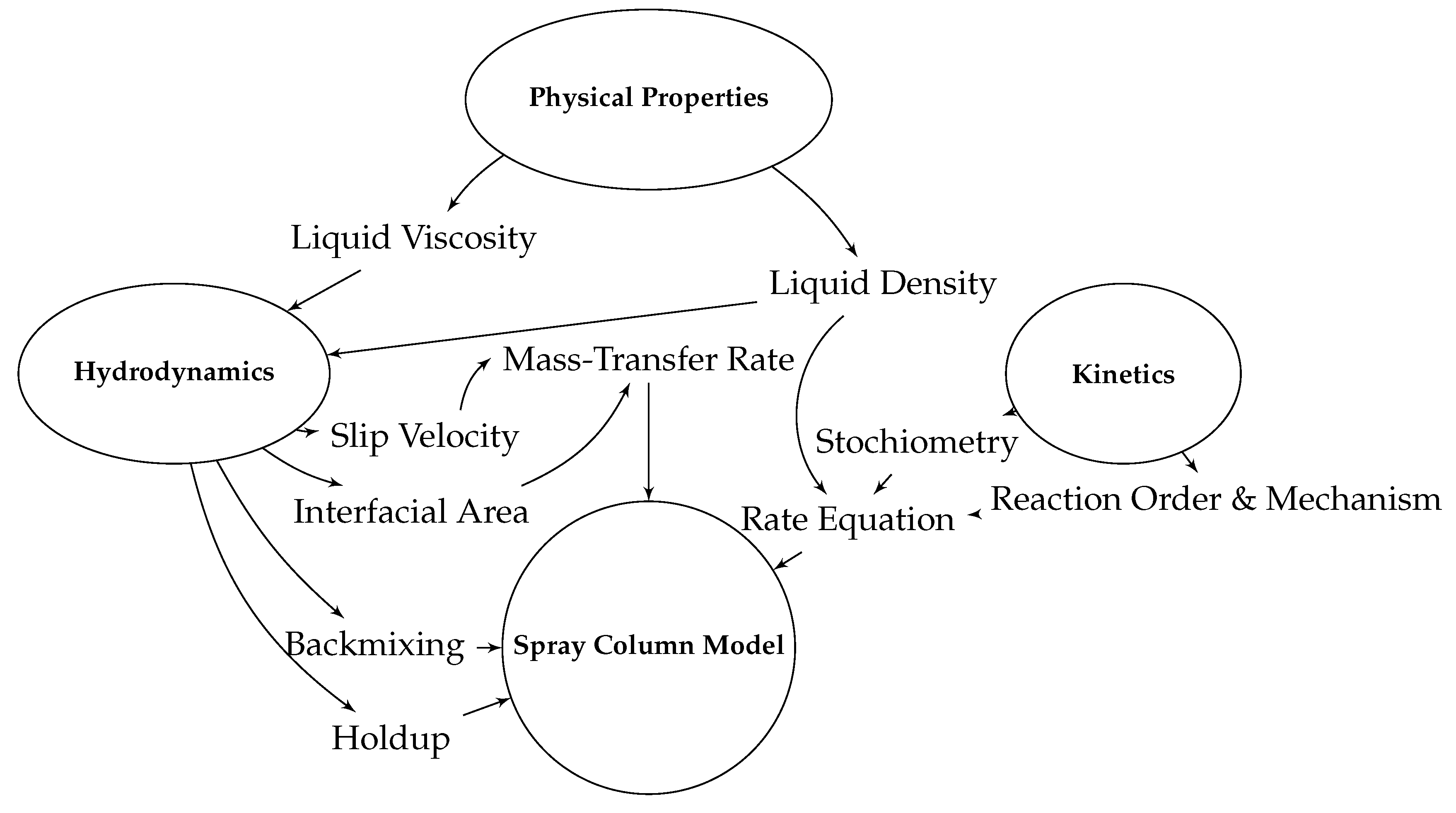
2. Methodology

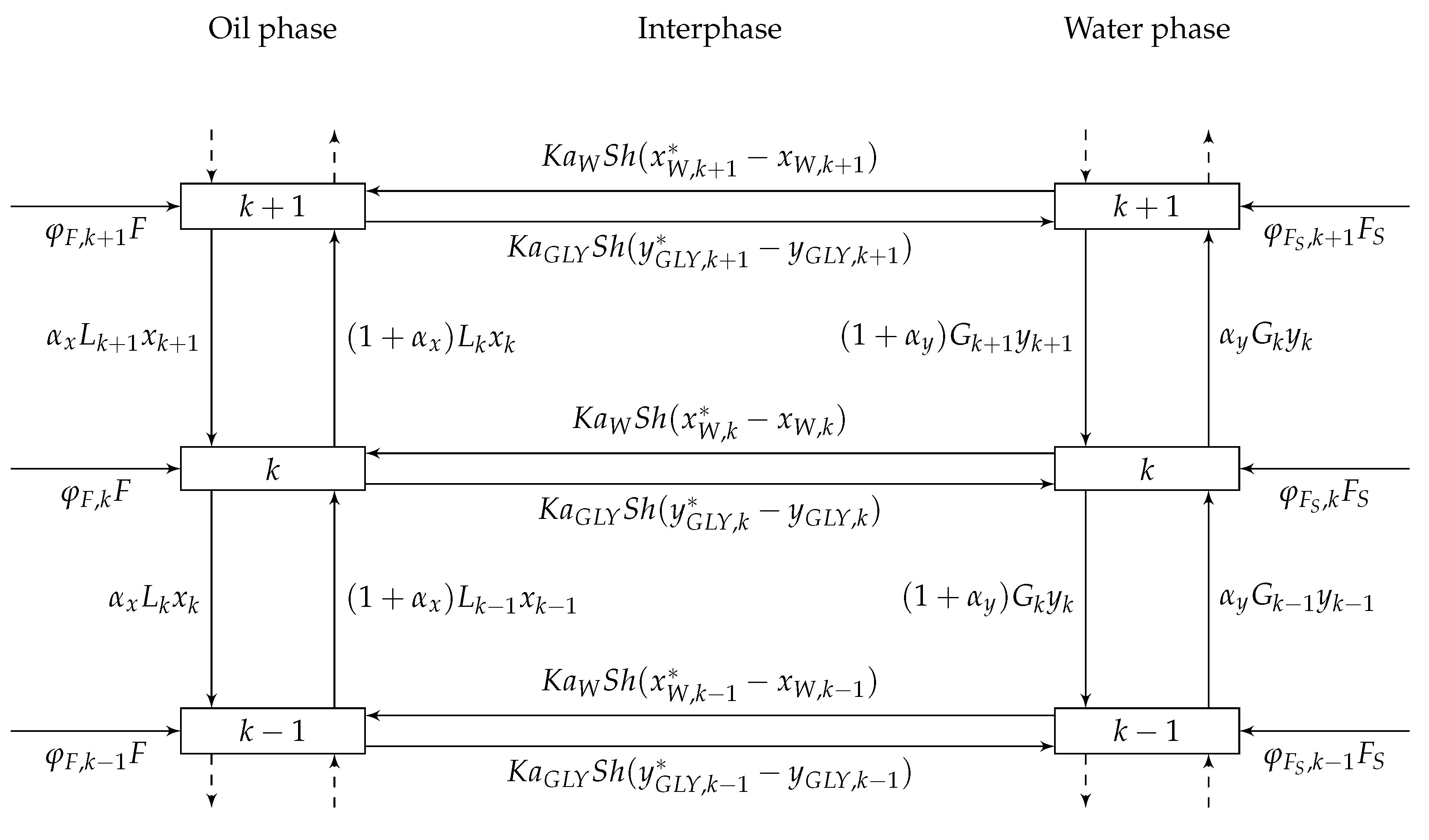
2.1. Process Model of a Counter-Current Spray Column

Figure 4 illustrates the interaction of the important properties and phenomena regarding a spray column [21]. The important physical and temperature-dependent properties in the spray column model are liquid density and liquid viscosity. Liquid density is used in the reaction rate term to calculate mass from volume. Liquid density and liquid viscosity enter also hydrodynamic calculations (correlations or computational fluid dynamics). The hydrodynamic calculations provide slip velocity and the interfacial area between the phases to the mass-transfer rate calculations. Furthermore, the backmixing and holdup values get directly included in the mass balance equations of the spray column model. The kinetics describe the stochiometry, reaction order and mechanism of the reaction system. These together with the liquid density go into the reaction rate expression which makes up the production or consumption terms in the component mass balances. The problem at hand is a boundary value problem at the height position $x=0$ ft (bottom of column) and $x=H$ (top of column). The system of partial differential equations (PDE) can be discretized with the finite volume method (FVM). The process model for hydrolyzing triglycerides with water to obtain fatty acids and glycerol is implemented in Fortran and interfaced through Python (via f90wrap [22]) to perform sensitivity analysis (with SALib [23]), re-parameterization and multi-criteria optimization (with SciPy [24]). A diagram of the FVM can be seen in Figure 5 and the equations are described in the next section.

2.1.1. Material Balance

The mass balance of triglycerides in the oil phase is described by the following equations:

$$\begin{array}{cc}\hfill m_k\frac{d{x}_{T{G}_i,k}}{dt}=0=& \stackrel{\mathrm{Backmixing}\mathrm{from}\mathrm{upper}\mathrm{stage}}{\overbrace{{\alpha }_x{L}_{k+1}{x}_{T{G}_i,k+1}}}-\stackrel{\mathrm{Comp}.\mathrm{flow}\mathrm{to}\mathrm{upper}\mathrm{stage}}{\overbrace{(1+{\alpha }_x)L_k{x}_{T{G}_i,k}}}\hfill \\ \hfill & -\underset{\mathrm{Backmixing}\mathrm{to}\mathrm{lower}\mathrm{stage}}{\underbrace{{\alpha }_x{L}_k{x}_{T{G}_i,k}}}+\underset{\mathrm{Comp}.\mathrm{flow}\mathrm{from}\mathrm{lower}\mathrm{stage}}{\underbrace{(1+{\alpha }_x)L_{k-1}{x}_{T{G}_i,k-1}}}\hfill \\ \hfill & -\underset{\mathrm{Consumption}\mathrm{of}\mathrm{TG}\mathrm{by}1\mathrm{st}\mathrm{order}\mathrm{reaction}}{\underbrace{k_{i}Sh{\rho }_{Oil}{x}_{T{G}_i,k}}}+\underset{\mathrm{Feed}\mathrm{on}\mathrm{stage}\mathrm{k}}{\underbrace{{\phi }_{k}F{x}_{F,T{G}_i}}}\hfill \end{array}$$

(1)

where $L_k$ and $G_k$ are the mass flowrates of oil and water in $\frac{lb}{h}$. h is the length of a stage or respectively a volumetric element since the modeled column does not feature any plates, stages or packings. The height of one element is $h=H/N$. $x_{T{G}_i,k}$ is the mass fraction of the triglyceride species TG${}_i$ in the volumetric element k. ${\alpha }_x$ is the backmixing coefficient for the continuous oil phase. $k_i$ is the reaction coefficient in respect to the triglyceride species i, S is the cross-sectional area of the column, h is the height of a volumetric elements, ${\rho }_{Oil}$ is the density of the oil phase at the given operating temperature and ${\varphi }_{F,k}$ is the fraction of the total feed flowrate F fed to the column at stage k.

The component balance of fatty acids in the oil phase is nearly identical to the triglyceride balance except for the positive production term:

$$\begin{array}{cc}\hfill m_k\frac{d{x}_{F{A}_i,k}}{dt}=0=& \stackrel{\mathrm{Backmixing}\mathrm{from}\mathrm{upper}\mathrm{stage}}{\overbrace{{\alpha }_x{L}_{k+1}{x}_{F{A}_i,k+1}}}-\stackrel{\mathrm{Comp}.\mathrm{flow}\mathrm{to}\mathrm{upper}\mathrm{stage}}{\overbrace{(1+{\alpha }_x)L_k{x}_{F{A}_i,k}}}\hfill \\ \hfill & -\underset{\mathrm{Backmixing}\mathrm{to}\mathrm{lower}\mathrm{stage}}{\underbrace{{\alpha }_x{L}_k{x}_{F{A}_i,k}}}+\underset{\mathrm{Comp}.\mathrm{flow}\mathrm{from}\mathrm{lower}\mathrm{stage}}{\underbrace{(1+{\alpha }_x)L_{k-1}{x}_{F{A}_i,k-1}}}\hfill \\ \hfill & +\underset{\mathrm{Production}\mathrm{of}\mathrm{FA}\mathrm{by}1\mathrm{st}\mathrm{order}\mathrm{reaction}}{\underbrace{\sum _{i=1}^{NoTG}\frac{k_{i}Sh{\rho }_{Oil}{x}_{T{G}_i,k}}{w_{FA,i}}}}+\underset{\mathrm{Feed}\mathrm{on}\mathrm{stage}\mathrm{k}}{\underbrace{{\phi }_{F,k}F{x}_{F,F{A}_i}}}\hfill \end{array}$$

(2)

$x_{FA,i,k}$ is the mass fraction of the fatty acid species in the volumetric element k. $w_{FA,i}$ (=1.05 for palmitic acid) is the mass related ratio to produce one unit fatty acid from one unit triglyceride.

The component balance of glycerol in the oil phase includes the mass transfer of glycerol between the oil and aqueous phase:

$$\begin{array}{cc}\hfill m_k\frac{d{x}_{GLY,k}}{dt}=0=& \stackrel{\mathrm{Backmixing}\mathrm{from}\mathrm{upper}\mathrm{stage}}{\overbrace{{\alpha }_x{L}_{k+1}{x}_{GLY,k+1}}}-\stackrel{\mathrm{Comp}.\mathrm{flow}\mathrm{to}\mathrm{upper}\mathrm{stage}}{\overbrace{(1+{\alpha }_x)L_k{x}_{GLY,k}}}\hfill \\ \hfill & -\underset{\mathrm{Backmixing}\mathrm{to}\mathrm{lower}\mathrm{stage}}{\underbrace{{\alpha }_x{L}_k{x}_{GLY,k}}}+\underset{\mathrm{Comp}.\mathrm{flow}\mathrm{from}\mathrm{lower}\mathrm{stage}}{\underbrace{(1+{\alpha }_x)L_{k-1}{x}_{GLY,k-1}}}\hfill \\ \hfill & +\underset{\mathrm{Production}\mathrm{of}\mathrm{GLY}\mathrm{by}1\mathrm{st}\mathrm{order}\mathrm{reaction}}{\underbrace{\sum _{i=1}^{NoTG}\frac{k_{i}Sh{\rho }_{Oil}{x}_{T{G}_i,k}}{w_{GLY}}}}\hfill \\ \hfill & -\underset{\mathrm{Mass}\mathrm{transfer}\mathrm{of}\mathrm{GLY}\mathrm{from}\mathrm{oil}\mathrm{to}\mathrm{aqueous}\mathrm{phase}}{\underbrace{K{a}_{GLY}Sh(y_{GLY,k}^{*}-y_{GLY,k})}}+\underset{\mathrm{Feed}\mathrm{on}\mathrm{stage}\mathrm{k}}{\underbrace{{\phi }_{F,k}F{x}_{F,GLY}}}\hfill \end{array}$$

(3)

where $w_{GLY}$ = 11.72 is the mass related ratio to produce one unit glycerol from one unit triglyceride.

For the component balance of glycerol in the aqueous phase the production term can be excluded since the reaction is only taking place in the oil phase:

$$\begin{array}{cc}\hfill m_k\frac{d{y}_{GLY,k}}{dt}=0=& \stackrel{\mathrm{Backmixing}\mathrm{from}\mathrm{lower}\mathrm{stage}}{\overbrace{{\alpha }_y{G}_{k-1}{y}_{GLY,k-1}}}-\stackrel{\mathrm{Comp}.\mathrm{flow}\mathrm{to}\mathrm{lower}\mathrm{stage}}{\overbrace{({\alpha }_y+1)G_k{y}_{GLY,k}}}\hfill \\ \hfill & -\underset{\mathrm{Backmixing}\mathrm{to}\mathrm{upper}\mathrm{stage}}{\underbrace{{\alpha }_y{G}_k{y}_{GLY,k}}}+\underset{\mathrm{Comp}.\mathrm{flow}\mathrm{from}\mathrm{upper}\mathrm{stage}}{\underbrace{({\alpha }_y+1)G_{k+1}{y}_{GLY,k+1}}}\hfill \\ \hfill & +\underset{\mathrm{Mass}\mathrm{transfer}\mathrm{of}\mathrm{GLY}\mathrm{from}\mathrm{oil}\mathrm{to}\mathrm{aqueous}\mathrm{phase}}{\underbrace{K{a}_{GLY}Sh(y_{GLY,k}^{*}-y_{GLY,k})}}+\underset{\mathrm{Steam}\mathrm{injection}\mathrm{on}\mathrm{stage}\mathrm{k}}{\underbrace{{\phi }_{S,k}{F}_S{y}_{S,GLY}}}\hfill \end{array}$$

(4)

The internal flowrate for the dispersed (water) phase is defined as:

$$\begin{array}{cc}\hfill \frac{d{G}_k}{dt}=0=& \stackrel{\mathrm{Backmixing}\mathrm{from}\mathrm{lower}\mathrm{stage}}{\overbrace{{\alpha }_y{G}_{k-1}}}-\stackrel{\mathrm{Total}\mathrm{mass}\mathrm{flow}\mathrm{to}\mathrm{lower}\mathrm{stage}}{\overbrace{(1+{\alpha }_y)G_k}}\hfill \\ \hfill & -\underset{\mathrm{Backmixing}\mathrm{to}\mathrm{upper}\mathrm{stage}}{\underbrace{{\alpha }_y{G}_k}}+\underset{\mathrm{Total}\mathrm{mass}\mathrm{flow}\mathrm{from}\mathrm{upper}\mathrm{stage}}{\underbrace{(1+{\alpha }_y)G_{k+1}}}\hfill \\ \hfill & -\underset{\mathrm{Mass}\mathrm{transfer}\mathrm{of}\mathrm{W}\mathrm{from}\mathrm{aqueous}\mathrm{to}\mathrm{oil}\mathrm{phase}}{\underbrace{K{a}_{W}Sh(x_{W,k}^{*}-x_{W,k})}}+\underset{\mathrm{Mass}\mathrm{transfer}\mathrm{of}\mathrm{GLY}\mathrm{from}\mathrm{oil}\mathrm{to}\mathrm{aqueous}\mathrm{phase}}{\underbrace{K{a}_{GLY}Sh(y_{GLY,k}^{*}-y_{GLY,k})}}\hfill \\ \hfill & +\underset{\mathrm{Steam}\mathrm{injection}\mathrm{on}\mathrm{stage}\mathrm{k}}{\underbrace{{\phi }_{S,k}{F}_S}}\hfill \end{array}$$

(5)

and the internal flowrate of the continuous (oil) phase reads:

$$\begin{array}{cc}\hfill \frac{d{L}_k}{dt}=0=& \stackrel{\mathrm{Backmixing}\mathrm{from}\mathrm{upper}\mathrm{stage}}{\overbrace{{\alpha }_x{L}_{k+1}}}-\stackrel{\mathrm{Total}\mathrm{mass}\mathrm{flow}\mathrm{to}\mathrm{upper}\mathrm{stage}}{\overbrace{(1+{\alpha }_x)L_k}}\hfill \\ \hfill & -\underset{\mathrm{Backmixing}\mathrm{to}\mathrm{lower}\mathrm{stage}}{\underbrace{{\alpha }_x{L}_k}}+\underset{\mathrm{Total}\mathrm{flow}\mathrm{from}\mathrm{lower}\mathrm{stage}}{\underbrace{(1+{\alpha }_x)L_{k-1}}}\hfill \\ \hfill & +\underset{\mathrm{Mass}\mathrm{transfer}\mathrm{of}\mathrm{W}\mathrm{from}\mathrm{aqueous}\mathrm{to}\mathrm{oil}\mathrm{phase}}{\underbrace{K{a}_{W}Sh(x_{W,k}^{*}-x_{W,k})}}\hfill \\ \hfill & -\underset{\mathrm{Mass}\mathrm{transfer}\mathrm{of}\mathrm{GLY}\mathrm{from}\mathrm{oil}\mathrm{to}\mathrm{aqueous}\mathrm{phase}}{\underbrace{K{a}_{GLY}Sh(y_{GLY,k}^{*}-y_{GLY,k})}}\hfill \\ \hfill & +\underset{\mathrm{Feed}\mathrm{on}\mathrm{stage}\mathrm{k}}{\underbrace{{\phi }_{F,k}F}}\hfill \end{array}$$

(6)

2.1.2. Phase Equilibrium

Based on the two film theory by Whitman [25], the equilibrium concentration of glycerol in the bulk aqueous phase at the interface $y_{GLY,k}^{*}$ can be expressed with the distribution ratio ${\psi }_{GLY}$ and the concentration in the bulk oil phase $x_{GLY,k}$:

$$y_{GLY,k}^{*}={\psi }_{GLY}{x}_{GLY,k}$$

(7)

Analogously, the equilibrium water fraction in the bulk oil phase is:

$$x_{W,k}^{*}={\psi }_W{y}_{W,k}={\psi }_W(1-y_{GLY,k})$$

(8)

The distribution can be calculated for example with the modified UNIFAC model but in this work we use the data for the distribution ratio of glycerol from the reference case for validation purposes and assume a distribution ratio of zero for water since no water is assumed to be soluble in the oil phase.

2.1.3. Solving the System of Equations

The system comprises $(NoC+2)\ast N$ equations with $(NoC+2)\ast N$ unknown variables being the fractions of the individual triglycerides and fatty acids in the continuous phase, the 2 glycerol fractions in the continuous and dispersed phase and the internal flowrates of both phases in each volumetric element. In this model we assume that each triglyceride has equivalent fatty acids sidechains and consequently one kind of triglyceride (1 mole) will react to one kind of fatty acid (3 moles). The continuous phase consists of triglycerides, fatty acids and glycerol. The dispersed phase is a mixture of glycerol and water since we assume no mass transfer of triglycerides and fatty acids between the oil and water interface. Thus, the water fraction in the dispersed phase can be derived from the glycerol fraction with the summation rule. Equations (1)–(3) are $(NoC-1)\ast N$ equations which gives $NoC\ast N$ equations when including equation set (4). The equation sets (5) and (6) add $2\ast N$ equations and the system has no degrees of freedom with the number of equations being the same as the number of unknown variables. The system of non-linear equations was solved with a global Newton method (NLEQ1 solver [26]). The base case is derived from experimental run number 6 conducted by Jeffreys et al.

2.2. Parameter Estimation via Differential Evolution (DE)

The initial estimates of the parameters for fitting purposes can be obtained via differential evolution (DE). The sum of squared error is evaluated during the parameter space search via DE by formulating the following objective function as the sum of squared differences between the predicted and measured data:

$$\begin{array}{cc}\hfill \sum _{i=1}^N& [{(y_{GLY,i}^{exp}-y_{GLY,i}^{sim})}^2+{(x_{GLY,i}^{exp}-x_{GLY,i}^{sim})}^2+{(\frac{G_{out,i}^{exp}-G_{out,i}^{sim}}{\mathrm{10,000}})}^2\hfill \\ \hfill & +{(\frac{L_{out,i}^{exp}-L_{out,i}^{sim}}{\mathrm{10,000}})}^2+{(\frac{G_{median,i}^{exp}-G_{median,i}^{sim}}{\mathrm{10,000}})}^2+{(\frac{L_{median,i}^{exp}-L_{median,i}^{sim}}{\mathrm{10,000}})}^2]\hfill \end{array}$$

(9)

where

$$G_{median,i}^{exp}=\frac{G_{in,i}^{exp}+G_{out,i}^{exp}}{2};L_{median,i}^{exp}=\frac{L_{in,i}^{exp}+L_{out,i}^{exp}}{2}$$

(10)

and

$$G_{median,i}^{sim}=\frac{G_{in,i}^{exp}+G_{out,i}^{sim}}{2};L_{median,i}^{sim}=\frac{L_{in,i}^{exp}+L_{out,i}^{sim}}{2}$$

(11)

A scaling factor had to be introduced for the mass flow rate differences to scale them to the value range of the mass fractions which lie between zero and one. DE is a stochastic direct search method by Storn and Price [27] and the algorithm is summarized in the following:

• Specify population size, number of generations, crossover probability, mutation factor.
• Initialize vector population where parameters are uniformly distributed within their bounds.
• Evaluate the objective (cost) function for all individuals (vectors) and store in the fitness variable.
• Generation loop until number of generations or fitness of cost function is reached:

  4.1.

  Mutation (Parameter mixing): Select a target vector, choose randomly three other vectors and create mutant vector $m=v_1+m_{factor}\ast (v_2-v_3)$ where $m_{factor}$ is called the mutant factor or differential weight.

  4.2.

  Recombination: Generate trial vector by a probabilistic swapping (crossover) of elements from current target vector with mutant vector.

  4.3.

  Replacement: Evaluate cost function and replace target vector with trial vector if the cost function is lower with the parameters from the trial vector.

• Parameter vector is returned with best fitness.

The model is then fitted with the parameters returned from DE routine as the first guess.

Table 3. Data used for parameter estimation.

Experimental Run	Input				Output
	${\mathit{L}}_{\mathit{in}}$ [lb/h]	${\mathit{G}}_{\mathit{in}}$ [lb/h]	${\mathit{\rho }}_{\mathit{Oil}}$ [lb/ft${}^3$]	m [−]	${\mathit{y}}_{\mathit{GLY}}$ [−]	${\mathit{x}}_{\mathit{GLY}}$ [−]	${\mathit{L}}_{\mathit{out}}$ [lb/h]	${\mathit{G}}_{\mathit{out}}$ [lb/h]	${\mathit{G}}_{\mathit{median}}$ [lb/h]	${\mathit{L}}_{\mathit{median}}$ [lb/h]
#1	7260	4600	45	10.32	0.1605	0.03	8050	3810	4205	7655
#2	6490	4440	45.05	9.56	0.1705	0.037	7180	3750	4095	6835
#3	6905	4300	45	11.38	0.189	0.027	7370	3835	4070	7140
#4	7400	3980	45.1	11.67	0.182	0.019	7770	3610	3795	7585
#5	6570	4480	44.9	8.32	0.227	0.027	7340	3710	4095	6955
#6	8175	4120	45.05	10.32	0.188	0.024	8900	3395	3760	8540

summarizes the data set from Jeffreys et al. which was used for the parameter estimation.

2.3. Multi-Criteria Optimization via Differential Evolution

Energy efficiency is an important aspect to make the economic performance of the spray column more viable and the direct injected steam consumes the largest energy share in this process [28]. The operating costs must be evaluated to optimize the amount of steam fed to the column and how to distribute it between the two steam inlets. The steam cost is summarized in

Table 4. Fixed and variable cost for high pressure (HP) steam production [29].

Cost	Unit	per 1000 lb Steam
Average boiler fuel	MMBtu	1.56
Fresh water	$	0.02
Water treatment cost	$	0.74
Water preheating and pumping	$	0.62
Deareation steam	$	1.10
FD fan	$	0.05
C${}_{var}$ (variable cost)	$	11.9
Boiler capital	MM$	20
R depraciation factor	% of capital	15
Maintenance cost	% of capital	2
Two employees	$/a	120,000
Employee cost factor	-	3
C${}_{fix}$ (fixed cost)	$	1.7
C${}_{ST}$ = C${}_{var}$ + C${}_{fix}$	$	13.6

Fuel price: 6 $/MMBtu.

with the total cost for steam production being 13.6 $ per 1000 lb steam [29].

A possible formulation of the environmental objective would be the Eco${}_{99}$-indicator [30] which describes the effect of a product or process on the environment over its life cycle in terms of three damage categories: Human health, ecosystem quality and resources. The three damage categories are then weighted and normalized to balance or put emphasis on short- or long-term perspectives [31,32]. The weighted values of the three damage categories are then summed up to retrieve the Eco${}_{99}$-indicator. The measure of the Eco${}_{99}$-indicator is performed in points whereas 1 Point aligns with one thousandth of the yearly environmental load of one average European inhabitant.

Table 5. Impact categories for the Eco${}_{99}$-indicator and normalized data for steel, steam and electricity [33].

Impact Category	Steel [Points/lb]	Steam [Points/lb]	Electricity [Points/kWh]
Human health (d = 1)
Carcinogenics	$2.867\times {10}^{-3}$	$5.352\times {10}^{-5}$	$4.360\times {10}^{-4}$
Climate change	$5.942\times {10}^{-3}$	$7.257\times {10}^{-4}$	$3.610\times {10}^{-6}$
Ionizing radiation	$2.046\times {10}^{-4}$	$5.126\times {10}^{-4}$	$8.240\times {10}^{-4}$
Ozone layer depletion	$2.064\times {10}^{-6}$	$9.525\times {10}^{-7}$	$1.210\times {10}^{-4}$
Respiratory effects	$3.633\times {10}^{-2}$	$3.570\times {10}^{-7}$	$1.350\times {10}^{-6}$
Ecosystem (d = 2)
Acidification	$1.229\times {10}^{-3}$	$5.488\times {10}^{-3}$	$2.810\times {10}^{-4}$
Ecotoxicity	$3.379\times {10}^{-2}$	$1.270\times {10}^{-3}$	$1.670\times {10}^{-4}$
Resources (d = 3)
Land occupation	$1.692\times {10}^{-3}$	$3.892\times {10}^{-5}$	$4.680\times {10}^{-4}$
Fossil fuels	$2.690\times {10}^{-2}$	$5.670\times {10}^{-2}$	$1.200\times {10}^{-3}$
Mineral extraction	$3.366\times {10}^{-2}$	$4.001\times {10}^{-6}$	$5.7\times {10}^{-6}$

lists the points per lb of the material/energy flows ${\beta }_b$ consumed by the spray column process. With this table an analysis for each damage category can be assessed as a function of the steel used for building the spray column, the steam consumed per year and the electricity needed for feeding the oil to the spray column. First the resource flows ${\beta }_b$ are multiplied with the individual impact category values and then summed up to obtain the impact of the resource usage on the damage category. Then the damage category values referenced to each resource are summed up and subsequently weighted and normalized to obtain the Eco${}_{99}$-indicator with the final summation. It is noted that the values in Table 5 are already normalized with respect to the steel, steam and electricity consumption. The equation for the indicator can be formulated as follows:

$${\mathrm{Eco}}_{99}=\sum _b\sum _d{\delta }_d{\omega }_d\sum _{k\in K}{\beta }_b{\alpha }_{b,k}$$

(12)

In conclusion, the description of the multi-criteria optimization problem is:

$$\begin{array}{ccc}\underset{\mathit{x}=\{F_S,{\varphi }_{F_S,k}\}}{\mathrm{minimize}}\hfill & \hfill & f(\mathit{x})=1/\mathrm{Profit}+{\mathrm{Eco}}_{99}+\mathrm{Product}\mathrm{Purity}\mathrm{Constraint}\hfill \\ \hfill & \hfill & =1/(\mathrm{Revenue}-\mathrm{TAC}-\mathrm{Raw}\mathrm{Material}\mathrm{Cos}\mathrm{t})+{\mathrm{Eco}}_{99}+\mathrm{Product}\mathrm{Purity}\mathrm{Constraint}\hfill \\ \mathrm{subject}\mathrm{to}\hfill & \hfill & F_S\in [50,5000]\hfill \\ \hfill & \hfill & {\varphi }_{F_S,100}\in [0.1,1]\hfill \\ \hfill & \hfill & {\varphi }_{F_S,70}=1-{\varphi }_{F_S,100}\hfill \end{array}$$

As we applied the DE algorithm to perform the parameter estimation, we apply the same algorithm to solve the optimization problem. The different criteria were scaled with constant factors. For both parameter estimation and multi-criteria optimization, the parameters of the DE algorithm were set to a population size of 15, a mutation range of 0.5–1.0 with dithering enabled and a recombination value of 0.7. These parameter values are the standard setting of the differential_evolution function in scipy.optimize. The two parameters subject to variation are G and ${\varphi }_{F_S,100}$ while the algorithm evaluates the objective function until it converges against a minimum and the stopping criterion is reached. The choice of DE as the optimization algorithm treats the rigorous model as a black box and gradient information do not have to be provided to the optimization routine. Furthermore, DE searches the problem space globally for finding the near optimal point and is a convenient method to receive first results before switching to e.g., gradient-based methods.

3. Results

Table 6. Model assumptions overview for the individual results sections.

Section	Model Assumptions	Significant Variables and/or Parameters
3.1. Model validation	- Constant internal flowrates	Process parameters by Jeffreys et al.
3.2. Global sensitivity analysis	- Constant internal flowrates	Phenomena-based parameters
3.3. Parameter estimation	- Variable internal flowrates	All relevant parameters (Table 8)
	- Solubility and mass transfer
	of water in and to oil phase
3.4. Multi-criteria optimization	- Variable internal flowrates	Process operation variables
	- No solubility and mass transfer
	of water in and to oil phase

highlights the model assumptions and significant variables or parameters for the individual results sections.

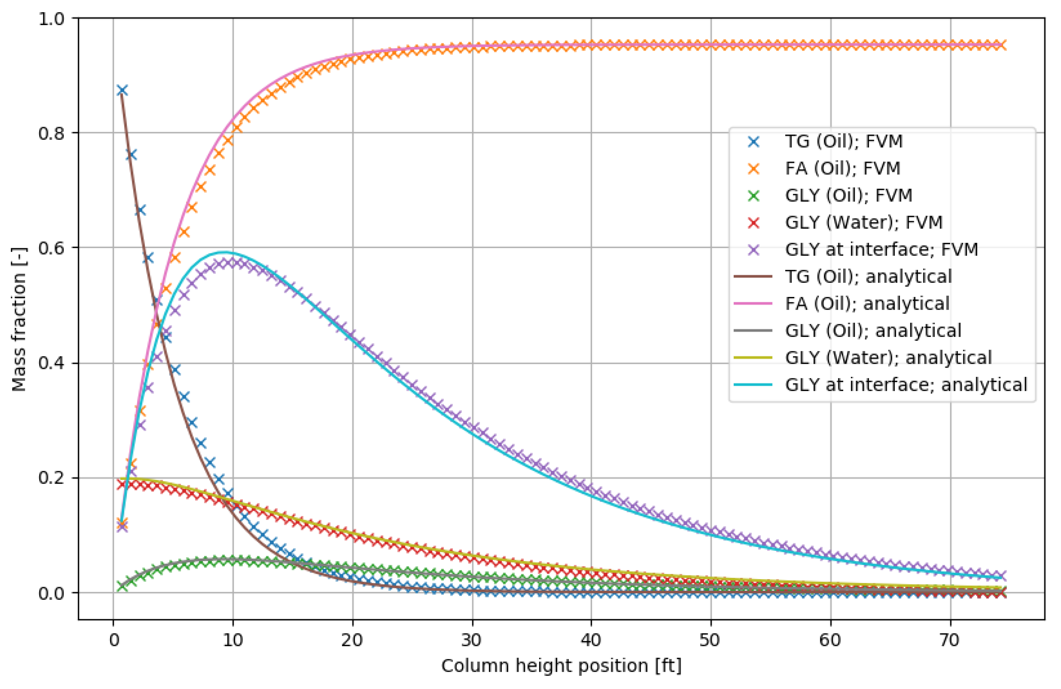
3.1. Model Validation

We compare the results of the proposed FVM in this work with the analytical model by Jeffreys et al. (experiment run no. 6) as seen in Figure 6. The parameters in

Table 7. Parameters for the counter-current oil-splitting column in English units and mass-based; experimental run number 6 by Jeffreys et al.

Parameter	Symbol	Nominal Value	Unit
Overall mass-transfer coefficient for glycerol	$Ka$	14.21	[lb/(ft${}^3$h)]
Cross-sectional area of tower	S	3.688	[ft${}^2$]
Mass flow of extract (aqueous phase)	G	3760	[lb/h]
Mass flow of raffinate (oil phase)	L	8540	[lb/h]
Glycerol distribution ratio/coefficient	${\psi }_{GLY}$	10.32	[−]
Forward reaction rate coefficient	k	10.2	[1/h]
Height of column	H	73.5	[ft]
Glycerol content in fat	$z_0/w_{GLY}$	0.0853	[−]
Liquid density of fat	${\rho }_{Oil}$	45.05	[lb/ft${}^3$]
Backmixing coefficient of cont. phase (oil)	${\alpha }_x$	0.0	[−]
Backmixing coefficient of disp. phase (water)	${\alpha }_y$	0.0	[−]

were used to validate the finite volume model against the analytical model by Jeffreys et al. The figure shows that the FVM aligns very well with the analytical model. The FVM presented in this paper was simulated with N = 100 volumetric elements. The glycerol content in the sweet water at the bottom of the column is 18.8%.

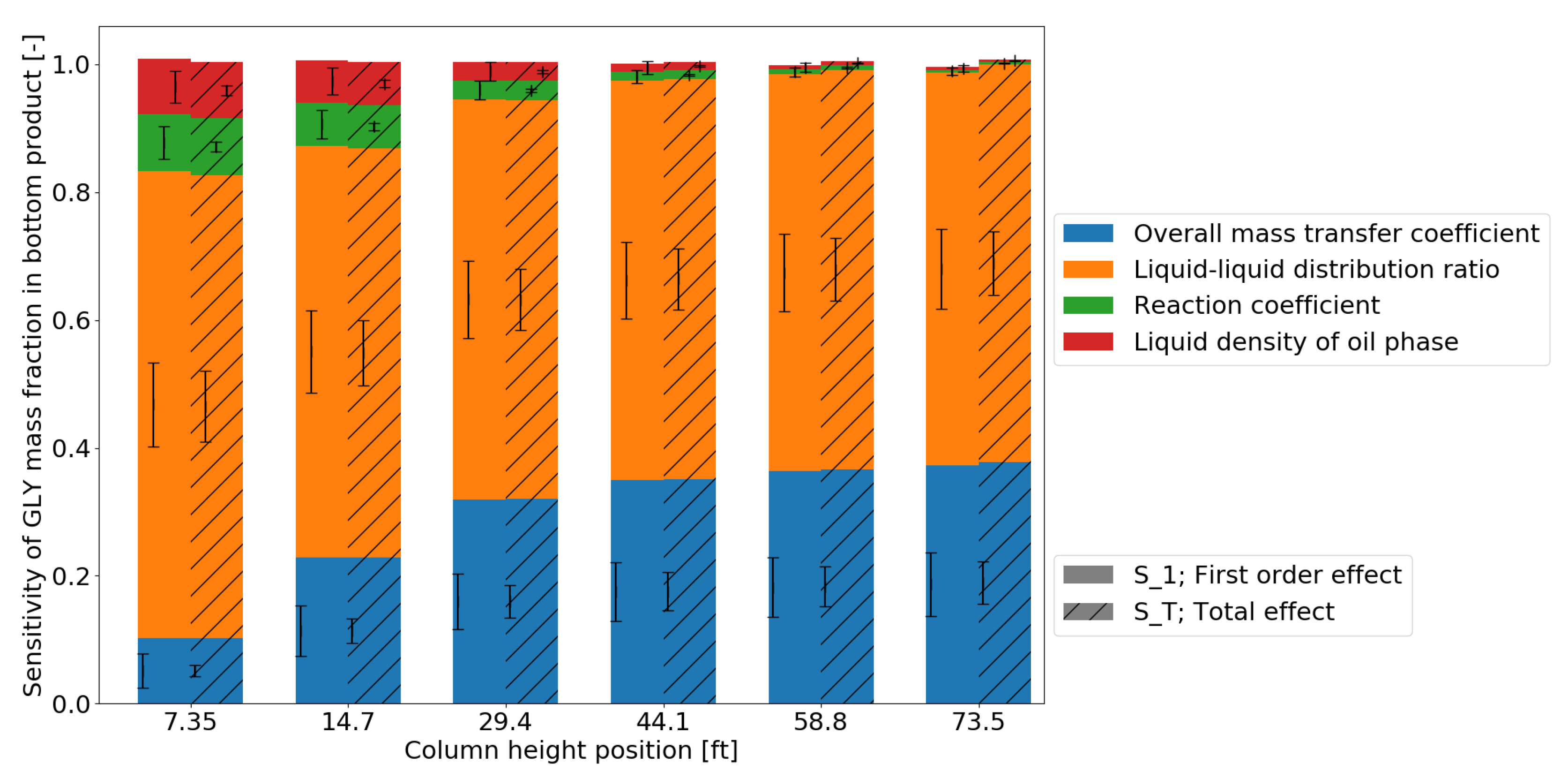
3.2. Global Sensitivity Analysis

Global sensitivity analysis allows identification and ranking of the important parameters in a unit operation model and can also be used to locate sensitive zones in e.g., columns and reactors. In this work we perform variance-based Sobol sensitivity analysis to evaluate physical (liquid density), thermodynamic (distribution ratio) and phenomena (kinetics and mass-transfer)-based properties with respect to the sensitivity of the glycerol content in the sweet water stream at the bottom of the column. Jeffreys et al. derive from their six experiments a variation in the overall mass-transfer coefficient for glycerol from 10.1 to 16.0 $\frac{lb}{f{t}^{2}h}$. These values can be calculated with the following equation:

$$K{a}_{GLY}=\frac{G_{median}}{HTU\ast S}$$

(13)

where the HTU (height to transfer unit) values have been documented by the reference paper. First we analyze the experimental data set where the mean value of $K{a}_{GLY}$ is 13.0 $\frac{lb}{f{t}^{2}h}$ with a standard deviation of 3.0 (±23%). The forward reaction rate is 10.2 $\frac{1}{h}$ with no further estimates or uncertainties given. They also report liquid density values for tripalmitin (C16:0) for each of the six experiments (Table 3) which we assume to be the density value at feed temperature on the first stage of the spray column. The mean of these six values is 45.016 $\frac{lb}{f{t}^3}$ with a standard deviation of 0.068 (0.15%) $\frac{lb}{f{t}^3}$. The mean of the distribution ratio is 10.26 with a standard deviation of 1.5 (14.6%). For the sensitivity analysis we define the means of the parameters as the values from the experimental run number 6 and define a normal distribution with a standard deviation of 5% for each parameter.

Variance-based sensitivity analysis with the Sobol method was performed for the analytical model and the results are shown in Figure 7. The results show that the distribution ratio and therefore the liquid–liquid phase equilibrium has the highest effect on the glycerol fraction in the bottom product. The overall mass-transfer coefficient follows as the second most important parameter and aligns with the literature that the unit operation at hand is a mass-transfer driven process. However, sensitivity of the glycerol fraction to the reaction rate coefficient is negligible. The reason is the very slow reaction regime [12]. The liquid density has no effect on the conversion from the starting material (TG and W) to the products (FA and GLY) although the liquid density uncertainty has been set higher than actually analyzed before. The liquid density nearly remains constant, even for different temperatures, as seen in the tabularized data (

Table A2. Liquid density values for caprylic, lauric and stearic triglycerides (TG) taken from the KT consortium lipid database [41,42].

Type of TG	Unit	225 ${}^{°}$C	276 ${}^{°}$C	280 ${}^{°}$C
C8:0 (Caprylic)	kg/m${}^3$	807.93	763.86	760.49
	lb/ft${}^3$	50.44	47.69	47.48
C12:0 (Lauric)	kg/m${}^3$	763.32	721.63	717.85
	lb/ft${}^3$	47.65	45.05	44.81
C18:0 (Stearic)	kg/m${}^3$	762.42	722.25	719.31
	lb/ft${}^3$	47.60	45.09	44.91

,

Table A3. Liquid density for vegetable oils [43].

Type of Oil	Unit	200 ${}^{°}$C
Canola oil	kg/m${}^3$	806.6
	lb/ft${}^3$	50.4
Corn oil	kg/m${}^3$	807.8
	lb/ft${}^3$	50.4
Peanut oil	kg/m${}^3$	801.5
	lb/ft${}^3$	50.0
Soybean oil	kg/m${}^3$	807.4
	lb/ft${}^3$	50.4

and

Table A4. Liquid density for coconut oil and water [13].

Substance	Unit	225 ${}^{°}$C	280 ${}^{°}$C
Coconut oil
	kg/m${}^3$	738.0025	690.5853
	lb/ft${}^3$	46.0720	43.1118
Water
	kg/m${}^3$	833.7878	747.7287
	lb/ft${}^3$	52.0517	46.6792

) in Appendix A, the liquid density change is relatively low for vegetable oils and pure triglycerides.

3.3. Parameter Estimation

To this end we assumed the same conditions as Jeffreys et al. did in their work. Since Rifai et al. show that variable internal flowrates cannot be assumed constant we defined variable continuous (oil) and dispersed (water) stream flowrates for the FVM. A parameter estimation must be performed for $K{a}_{GLY}$ and the second mass-transfer coefficient describing the mass transfer between the oil and water phase $K{a}_W$. The forward reaction constant k, the backmixing coefficients (${\alpha }_x$ and ${\alpha }_y$) and distribution ratios (${\psi }_{GLY}$ and ${\psi }_W$) have also been included as parameters to be estimated. As already highlighted in Table 6, the model has been extended with the mass transfer and solubility of water to and in the oil phase. The results of the parameter estimation via DE are summarized in

Table 8. Results of parameter estimation via DE for the FVM with variable internal water and oil flowrates.

Parameter	Re-Parameterized Model		Jeffreys et al.
$K{a}_{GLY}$	43.64		19.06
$K{a}_W$	0.19		-
k	77.14		10.2
${\alpha }_x$	0.37		0.9
${\alpha }_y$	0.19		0.1
${\psi }_{GLY}$	64.17		10.32
${\psi }_W$	27.40		-
Experiment	$y_{GLY}^{sim}$ [−]	$y_{GLY}^{exp}$ [−]	Deviation from exp. [%]	$G_{out}^{sim}$ [lb/h]	$G_{out}^{exp}$ [lb/h]	Deviation from exp. [%]
1	0.1708	0.1605	6.4174	3879	3810	1.8110
2	0.1832	0.1705	7.4487	3741	3750	−0.24
3	0.2072	0.189	9.6296	3686	3835	−3.8853
4	0.2076	0.182	14.0659	3294	3610	−8.7535
5	0.2265	0.227	−0.2203	3983	3710	7.3585
6	0.2030	0.188	7.9787	3436	3395	1.2077
	$x_{GLY}^{sim}$ [−]	$x_{GLY}^{exp}$ [−]		$L_{out}^{sim}$ [lb/h]	$L_{out}^{exp}$ [lb/h]
1	0.0000	0.03	−100	7981	8050	-0.8571
2	0.0000	0.037	−100	7189	7180	0.1253
3	0.0000	0.027	−100	7519	7370	2.0217
4	0.0000	0.019	−100	8086	7770	4.0669
5	0.0000	0.027	−100	7067	7340	−3.7193
6	0.0000	0.024	−100	8859	8900	−0.4607
	$G_{median}^{sim}$ [lb/h]	$G_{median}^{exp}$ [lb/h]		$L_{median}^{sim}$ [lb/h]	$L_{median}^{exp}$ [lb/h]
1	4236	4205	0.7372	7586	7655	−0.9014
2	4088	4095	−0.1709	6798	6835	−0.5413
3	3990	4070	−1.9656	7169	7140	0.4062
4	3634	3795	−4.2424	7709	7585	1.6348
5	4228	4095	3.2479	6764	6955	−2.7462
6	3775	3760	0.3989	8487	8540	−0.6206

and compared to the data from Jeffreys et al. who used the individual experimental runs to obtain the mass-transfer coefficient of glycerol.

We used all six experiments for fitting the parameters $K{a}_{GLY}$, $K{a}_W$, k, ${\alpha }_x$, ${\alpha }_y$, ${\psi }_{GLY}$ and ${\psi }_W$ where the first guess for $L_H$ and $G_0$ had to be provided accordingly. The covariance matrix is:

$$\mathbf{Cov}=\begin{array}{cc}\begin{array}{ccccccc}\hspace{1em}\hspace{1em}\hspace{1em}K{a}_{GLY}\hspace{1em}\hspace{1em}\hspace{1em}\hspace{1em}& K{a}_W\hspace{1em}\hspace{1em}\hspace{1em}\hspace{1em}& k\hspace{1em}\hspace{1em}\hspace{1em}\hspace{1em}& {\alpha }_x\hspace{1em}\hspace{1em}\hspace{1em}\hspace{1em}& {\alpha }_y\hspace{1em}\hspace{1em}\hspace{1em}\hspace{1em}& {\psi }_{GLY}\hspace{1em}\hspace{1em}\hspace{1em}\hspace{1em}& {\psi }_W\hspace{1em}\hspace{1em}\hspace{1em}\hspace{1em}\end{array}& \\ \left(\begin{array}{ccccccc}8.84\times {10}^9& -7.16\times {10}^{10}& -8.0\times {10}^9& -2.84\times {10}^7& -3.63\times {10}^6& -3.16\times {10}^{10}& 1.04\times {10}^{13}\\ -7.16\times {10}^{10}& 6.61\times {10}^{10}& 2.40\times {10}^8& 3.14\times {10}^7& 5.95\times {10}^{11}& 2.62\times {10}^{11}& -8.67\times {10}^{13}\\ -8.00\times {10}^9& 2.40\times {10}^8& 7.35\times {10}^9& 2.65\times {10}^7& 3.46\times {10}^6& 2.91\times {10}^{10}& -9.62\times {10}^{12}\\ -2.84\times {10}^7& 3.14\times {10}^7& 2.65\times {10}^7& 9.74\times {10}^4& 1.30\times {10}^4& 1.05\times {10}^8& -3.49\times {10}^{10}\\ -3.63\times {10}^6& 5.95\times {10}^{11}& 3.46\times {10}^6& 1.30\times {10}^4& 1.87\times {10}^3& 1.37\times {10}^7& -4.58\times {10}^9\\ -3.16\times {10}^{10}& 2.62\times {10}^{11}& 2.91\times {10}^{10}& 1.10\times {10}^8& 1.37\times {10}^7& 1.15\times {10}^{11}& -3.81\times {10}^{13}\\ 1.04\times {10}^{13}& -8.67\times {10}^{13}& -9.62\times {10}^{12}& -3.49\times {10}^{10}& -4.58\times {10}^9& -3.81\times {10}^{13}& 1.26\times {10}^{16}\end{array}\right)& \begin{array}{c}K{a}_{GLY}\\ K{a}_W\\ k\\ {\alpha }_x\\ {\alpha }_y\\ {\psi }_{GLY}\\ {\psi }_W\end{array}\end{array}$$

(14)

The standard deviation of the parameters’ mean value is calculated from the covariance matrix and results in:

$$\mathit{\sigma }=\sqrt{\mathrm{diag}(\mathbf{Cov})}=\left(\begin{array}{c}9.40e4\\ 7.71e5\\ 8.58e4\\ 3.12e2\\ 4.33e1\\ 3.39e5\\ 1.12e8\end{array}\right)$$

(15)

The results show that more experimental data is necessary to provide a satisfactory parameter estimation. Furthermore, changing the kinetic model to a second order reaction or other reaction scheme may enhance the parameter estimation but if one wants to include a second order reaction model then measurements of the water concentration in the oil phase are needed (see kinetic term for Rifai et al. in Table 2).

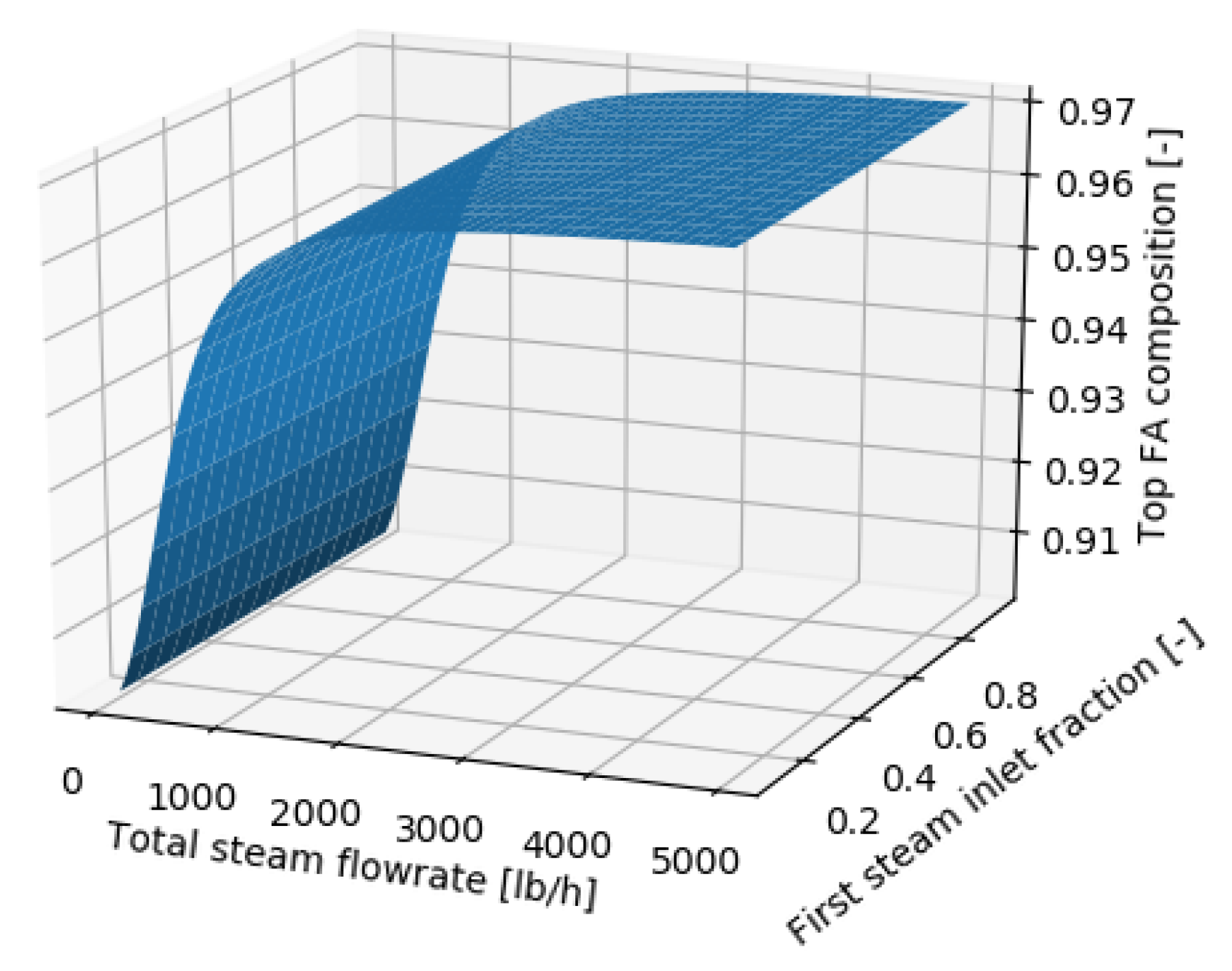
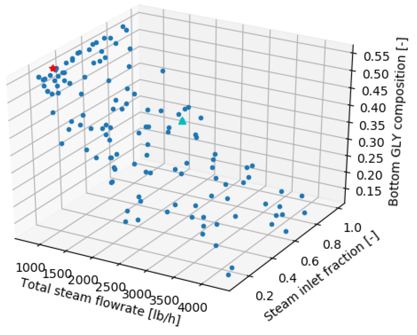
3.4. Multi-Criteria Optimization

Before discussing the results for the multi-criteria optimization we look at the response surfaces of the FVM for the fatty acid and glycerol fractions at the top and bottom of the column. As Figure 8 shows the glycerol fraction increases with decreasing steam flowrates since the glycerol will be more concentrated with lower steam flow rates until it reaches a maximum and then decreases because no water is available for the reaction. We can see a very slight increase of the glycerol fraction when we increase the amount of water which is fed through the first inlet and consequently less water will pass the second steam inlet.

Simultaneously when increasing the water flowrate, we can see in Figure 9 that the fatty acid fraction reaches a plateau at about 2000 $\frac{lb}{h}$. Meaning that the water flowrate of 4120 $\frac{lb}{h}$ of the base case is too high and dilutes on the one side the glycerol content in the sweet water product and on the other side it does not increase the fatty acid content in the top product significantly. The multi-criteria optimization will therefore find the point where the glycerol and fatty acid fractions are balanced out with respect to the objective function.

In regards to the revenue which can be generated from the fatty acid and sweet water product streams, we assume that the product streams will be further purified and therefore set the prices for the palmitic acid product at the top of the spray column to be 0.71 $\frac{US\$}{lb}$ [34] which is the price for high grade palmitic acid. The sweet water product at the bottom of column is assumed to be further purified to high grade glycerol with a price of 0.085 $\frac{US\$}{lb}$ [35]. The raw material price of the vegetable oil is 0.2359 $\frac{US\$}{lb}$ [36]. The size of the column is 73.5 ft in height [10], 2.16696 ft in diameter [13] and the column wall thickness is assumed 0.01001 ft (3.05 mm). The material is stainless steel 316 (${\rho }_{SS316}$ = 229.9 $\frac{kg}{f{t}^3}$ = 506.84 $\frac{lb}{f{t}^3}$). For calculating the capital cost, we assume the spray column being the shape of a cylinder and thus the weight of the column is 5.11 $f{t}^3$ times 506.84 $\frac{lb}{f{t}^3}$ which gives 116,522.5 lb. The price of stainless steel 316 is 4227 $\frac{US\$}{t}$[37] and thus we obtain a capital cost of 4966 US$ for the material of the spray column. The Eco${}_{99}$-indicator calculation covers the used steel material, steam generation and the electricity for pumping. This results in the following equation for the Eco${}_{99}$-indicator:

$${\mathrm{Eco}}_{99}=\sum _b\sum _d{\omega }_d\sum _k{\beta }_{Steel}\ast {\alpha }_{Steel,k}+\sum _k{\beta }_{Steam}\ast {\alpha }_{Steam,k}+\sum _k{\beta }_{Electricity}\ast {\alpha }_{Electricity,k}$$

(16)

where ${\beta }_{Steel}$ = 1174.8 kg and the pump duty for the feed is ${\beta }_{Electricity}$ = 440.59 kWh. The steam flowrate is a decision variable subject to change during the DE algorithm. The weighting factors ${\omega }_d$ are set in respect to a hierarchist perspective (human health = 40%, ecosystem quality = 40% and resources = 20%). The results (

Table 9. Results of multi-criteria optimization.

Input and Objective	Unit	Value	Input Bounds
Input
Steam flowrate	lb/h	786.55	[50, 5000]
First steam inlet fraction	-	0.27	[0.1, 1.0]
Objective
Revenue	$/a	47,410,513
Total annual cost (TAC)	$/a	94,076
Raw material cost	$/a	17,452,458
Profit	$/a	29,863,978
Eco99 indicator	Points	22,316

) show that the optimization minimizes the steam flowrate to a point where the product constraint is still satisfied. This results in a lower conversion and the fatty acid fraction in the top product is 0.9502 (Figure 10) while the glycerol fraction in sweet water is 0.5571 (Figure 11) with a top product flowrate of 8044 $\frac{lb}{h}$ and a sweet water flowrate of 1283 $\frac{lb}{h}$.

4. Discussion

The results show that a FVM can be used to describe the spray column unit operation. More experimental data is needed to fully validate the FVM. The experimental setup of a counter-current spray column presented by Cadavid et al. [38] can be established to obtain the necessary data. Combined with the work by Forero-Hernandez et al. [39] to perform rigorous kinetic data analysis and the model presented here, important information about the hydrolysis of vegetable oils in spray columns can be obtained. Future research should be made regarding computational fluid dynamics (CFD) to describe the hydrodynamics in the spray column. This will allow the generation of surrogate functions from the computational cost-intensive CFD model and include them in the FVM model. The multi-criteria optimization formulation can also be re-formulated as a multi-objective optimization problem which gives interesting possibilities in process design and control research [40]. Future research endeavors are also advised to include an energy balance in the model formulation for taking the temperature gradient over the column height into account.

5. Conclusions

This work presents a FVM for a counter-current spray column to describe the hydrolysis of vegetable oils. The presented model can be adapted to different spray column designs/configurations and gives the engineer a valuable tool to validate, analyze and optimize an industrial scale spray column. The possibility to perform parameter estimation is given if experimental data from an existing plant is provided. Through multi-criteria optimization sustainable process design can be achieved by including sustainability indicators such as the Eco${}_{99}$-indicator into the objective function. The model enables the testing and analysis of different scenarios and allows communication with packages and tools in line with the concept of digital industry 4.0.

References

1. Grand View Research. Oleochemicals Market Size, Share & Trends Analysis Report by Product (Fatty Acid, Glycerol, Fatty Alcohol), by Region (APAC, MEA, Europe, North America, CSA), and Segment Forecasts, 2018–2025; Technical Report; Grand View Research: San Francisco, CA, USA, 2018. [Google Scholar]
2. Searchinger, T.; Heimlich, R.; Houghton, R.A.; Dong, F.; Elobeid, A.; Fabiosa, J.; Tokgoz, S.; Hayes, D.; Yu, T.H. Use of U.S. Croplands for Biofuels Increases Greenhouse Gases Through Emissions from Land-Use Change. Science 2008, 319, 1238–1240. [Google Scholar] [CrossRef] [PubMed]
3. Fargione, J.; Hill, J.; Tilman, D.; Polasky, S.; Hawthorne, P. Land Clearing and the Biofuel Carbon Debt. Science 2008, 319, 1235–1238. [Google Scholar] [CrossRef] [PubMed]
4. Martinez-Guerra, E.; Gude, V.G. Assessment of Sustainability Indicators for Biodiesel Production. Appl. Sci. 2017, 7, 869. [Google Scholar] [CrossRef]
5. Patil, T.A.; Raghunathan, T.S.; Shankar, H.S. Thermal Hydrolysis of Vegetable Oils and Fats. 2. Hydrolysis in Continuous Stirred Tank Reactor. Ind. Eng. Chem. Res. 1988, 27, 735–739. [Google Scholar] [CrossRef]
6. Forero-Hernandez, H.; Jones, M.N.; Sarup, B.; Jensen, A.D.; Sin, G. A simplified kinetic and mass transfer modelling of the thermal hydrolysis of vegetable oils. Comput. Aided Chem. Eng. 2017, 40, 1177–1182. [Google Scholar] [CrossRef]
7. Lascaray, L. Mechanism of Fat Splitting. Ind. Eng. Chem. 1949, 41, 786–790. [Google Scholar] [CrossRef]
8. Lascaray, L. Industrial Fat Splitting. J. Am. Oil Chem. Soc. 1952, 29, 362–366. [Google Scholar] [CrossRef]
9. Sturzenegger, A.; Sturm, H. Hydrolysis of Fats and High Temperatures. Ind. Eng. Chem. 1951, 43, 510–515. [Google Scholar] [CrossRef]
10. Jeffreys, G.V.; Jenson, V.G.; Miles, F.R. The Analysis of a Continiuous Fat-Hydrolysing Column. Trans. Inst. Chem. Eng. 1961, 39, 389–396. [Google Scholar]
11. Rifai, M.; Nashaie, S.; Kafafi, A. Analysis of a Countercurrent Tallow-Splitting Column. Trans. Inst. Chem. Eng. 1977, 55, 59–63. [Google Scholar]
12. Namdev, P.D.; Patil, T.A.; Raghunathan, T.S.; Shankar, H.S. Thermal Hydrolysis of Vegetable Oils and Fats. 3. An Analysis of Design Alternatives. Ind. Eng. Chem. Res. 1988, 27, 739–743. [Google Scholar] [CrossRef]
13. Attarakih, M.; Albaraghthi, T.; Abu-Khader, M.; Al-Hamamre, Z.; Bart, H. Mathematical modeling of high-pressure oil-splitting reactor using a reduced population balance model. Chem. Eng. Sci. 2012, 84, 276–291. [Google Scholar] [CrossRef]
14. Alenezi, R.; Leeke, G.A.; Santos, R.C.D.; Khan, A.R. Hydrolysis kinetics of sunflower oil under subcritical water conditions. Chem. Eng. Res. Des. 2009, 87, 867–873. [Google Scholar] [CrossRef]
15. Patil, T.A.; Butala, D.N.; Raghunathan, T.S.; Shankar, H.S. Thermal Hydrolysis of Vegetable Oils and Fats. 1. Reaction kinetics. Ind. Eng. Chem. Res. 1988, 27, 727–735. [Google Scholar] [CrossRef]
16. Aniya, V.K.; Muktham, R.K.; Alka, K.; Satyavathi, B. Modeling and simulation of batch kinetics of non-edible karanja oil for biodiesel production. Fuel 2015, 161, 137–145. [Google Scholar] [CrossRef]
17. Mills, V.; McClain, H.K. Fat Hydrolysis. Ind. Eng. Chem. 1949, 41, 1982–1985. [Google Scholar] [CrossRef]
18. Minard, G.W.; Johnson, A.I. Limiting Flow and Holdup in a Spray Extraction Column. Chem. Eng. Prog. 1952, 48. [Google Scholar]
19. Beyaert, B.O.; Lapidus, L.; Elgin, J.C. The Mechanics of Vertical Moving Liquid-Liquid Fluidized Systems: II. Countercurrent Flow. AIChE J. 1961, 7, 46–48. [Google Scholar] [CrossRef]
20. Van Egmond, L.C.; Goossens, M.L. Berekningen aan Axiale Dispersie in een Operationele Vetsplitter; Technical Report; Laboratorium voor Chemische Technologie: Delft, The Netherlands, 1982. [Google Scholar]
21. Ettouney, R.S.; El-Rifai, M.A.; Ghallab, A.O.; Anwar, A.K. Mass Transfer Fluid Flow Interactions in Perforated Plate Extractive Reactors. Sep. Sci. Technol. 2015, 50, 1794–1805. [Google Scholar] [CrossRef]
22. Kermode, J. f90wrap. Available online: https://github.com/jameskermode/f90wrap (accessed on 9 March 2018).
23. Herman, J.; Usher, W. SALib: An open-source Python library for sensitivity analysis. J. Open Source Softw. 2017, 2, 97. [Google Scholar] [CrossRef]
24. Virtanen, P.; Gommers, R.; Oliphant, T.E.; Haberland, M.; Reddy, T.; Cournapeau, D.; Burovski, E.; Peterson, P.; Weckesser, W.; Bright, J.; et al. SciPy 1.0–Fundamental Algorithms for Scientific Computing in Python. 2019. Available online: https://arxiv.org/abs/1907.10121 (accessed on 9 March 2018).
25. Whitman, W.G. The two film theory of gas absorption. Int. J. Heat Mass Transf. 1962, 5, 429–433. [Google Scholar] [CrossRef]
26. Nowak, U.; Weimann, L. A Family of Newton Codes for Systems of Highly Nonlinear Equations; Technical Report; Konrad-Zuse-Zentrum für Informationstechnik Berlin: Berlin, Germany, 1991. [Google Scholar]
27. Storn, R.; Price, K. Differential Evolution—A Simple and Efficient Heuristic for global Optimization over Continuous Spaces. J. Glob. Optim. 1997, 11, 341–359. [Google Scholar] [CrossRef]
28. Wang, W.C.; Turner, T.L.; Roberts, W.L.; Stikeleather, L.F. Direct injection of superheated steam for continuous hydrolysis reaction. Chem. Eng. Process. Process Intensif. 2012, 59, 52–59. [Google Scholar] [CrossRef]
29. Determining True Steam Prices. In Energy and Process Optimization for the Process Industries; John Wiley & Sons, Ltd.: Hoboken, NJ, USA, 2013; Chapter 17; pp. 366–385. [CrossRef]
30. Goedkoop, M.; Spriensma, R. The Eco-indicator99: A Damage Oriented Method for Life Cycle Impact Assessment: Methodology Report; Technical Report; PRe Consultants B.V.: Amersfoort, The Netherlands, 2001. [Google Scholar]
31. Thompson, M.; Ellis, R.; Wildavsky, A. Cultural Theory; Westview Press: Boulder, CO, USA, 1990. [Google Scholar]
32. Hofstetter, P. Perspectives in Life Cycle Impact Assessment; Springer: Zurich, Switzerland, 1998. [Google Scholar] [CrossRef]
33. Rangaiah, G.P.; Sharma, S. Differential Evolution in Chemical Engineering; World Scientific: Singapore, 2017. [Google Scholar] [CrossRef]
34. Landress, L. Fatty Acids (North America); Technical Report; ICIS Pricing: London, UK, 2014. [Google Scholar]
35. Landress, L. Glycerine (US Gulf); Technical Report; ICIS Pricing: London, UK, 2014. [Google Scholar]
36. Malaysian Palm Oil Council (Oil). CPO vs SBO Prices. 2019. Available online: http://mpoc.org.my/daily-palm-oil-price/ (accessed on 9 March 2018).
37. International, M. MEPS-World Stainless Steel Prices. 2018. Available online: http://www.meps.co.uk/world-price.htm#STEEL%20PRICE%20TABLES (accessed on 9 March 2018).
38. Cadavid, J.; Godoy-Silva, R.; Narvaez, P.; Camargo, M.; Fonteix, C. Biodiesel production in a counter-current reactive extraction column: Modelling, parametric identification and optimisation. Chem. Eng. J. 2013, 228, 717–723. [Google Scholar] [CrossRef]
39. Forero-Hernandez, H.; Jones, M.N.; Sarup, B.; Jensen, A.D.; Abildskov, J.; Sin, G. Comprehensive development, uncertainty and sensitivity analysis of a model for the hydrolysis of rapeseed oil. Comput. Chem. Eng. 2020, 133, 106631. [Google Scholar] [CrossRef]
40. Rashid, M.M.; Mhaskar, P.; Swartz, C.L.E. Handling multi-rate and missing data in variable duration economic model predictive control of batch processes. AIChE J. 2017, 63, 2705–2718. [Google Scholar] [CrossRef]
41. Diaz-Tovar, C.A.; Gani, R.; Sarup, B. Computer-Aided Modeling of Lipid Processing Technology. Ph.D. Thesis, Technical University of Denmark (DTU), Lyngby, Denmark, 2011. [Google Scholar]
42. Perederic, O. Systematic Computer Aided Methods and Tools for Lipid Process Technology. Ph.D. Thesis, Technical University of Denmark (DTU), Lyngby, Denmark, 2018. [Google Scholar]
43. Sahasrabudhe, S.N.; Rodriguez-Martinez, V.; O’Meara, M.; Farkas, B.E. Density, viscosity, and surface tension of five vegetable oils at elevated temperatures: Measurement and modeling. Int. J. Food Prop. 2017, 20, 1965–1981. [Google Scholar] [CrossRef] [Green Version]
Figure 1. Hydrolysis reaction of triglycerides with water to give fatty acids and glycerol.
Processes 07 00881 g001
Figure 2. Hydrolysis of triglycerides in three-step reaction periods.
Processes 07 00881 g002
Figure 3. Counter-current spray column.
Processes 07 00881 g003
Figure 4. Properties and phenomena interaction in respect to a counter-current liquid–liquid spray column under subcritical conditions adapted from [21].
Processes 07 00881 g004
Figure 5. Schematic diagram of the finite volume model for the counter-current spray column.
Processes 07 00881 g005
Figure 6. Validation of finite volume model (constant internal flows) with analytical model from Jeffreys et al.
Processes 07 00881 g006
Figure 7. Sensitivity analysis of analytical model.
Processes 07 00881 g007
Figure 8. Response surface for glycerol fraction in bottom product with variable total steam flowrate and two inlets for the steam injection.
Processes 07 00881 g008
Figure 9. Response surface for fatty acid fraction in top product with variable water flowrate and two inlets for steam.
Processes 07 00881 g009
Figure 10. Pareto frontier for fatty acid fraction in product stream in respect to steam flowrate and inlet fraction (red point is the final solution of the differential evolution procedure; green triangle is the starting point).
Processes 07 00881 g010
Figure 11. Pareto frontier for glycerol fraction at bottom of the column in respect to steam flowrate and inlet fraction (red point is the final solution of the differential evolution procedure, green triangle is the starting point).
Processes 07 00881 g011