Article

Systematic Selection of Green Solvents and Process Optimization for the Hydroformylation of Long-Chain Olefines

1
Otto von Guericke University Magdeburg, Chair for Automation/Modeling, Universitätsplatz 2, 39106 Magdeburg, Germany
2
Otto von Guericke University Magdeburg, Chair for Process Systems Engineering, Universitätsplatz 2, 39106 Magdeburg, Germany
3
Max Planck Institute for Dynamics of Complex Technical Systems, Process Systems Engineering Group, Sandtorstraße 1, 39106 Magdeburg, Germany
4
Max Planck Institute for Dynamics of Complex Technical Systems, Process Synthesis and Dynamics Group, Sandtorstraße 1, 39106 Magdeburg, Germany
*
Authors to whom correspondence should be addressed.
Submission received: 15 October 2019 / Revised: 20 November 2019 / Accepted: 22 November 2019 / Published: 26 November 2019
(This article belongs to the Special Issue Advanced Methods in Process and Systems Engineering)

Abstract

:
Including ecologic and environmental aspects in chemical engineering requires new methods for process design and optimization. In this work, a hydroformylation process of long-chain olefines is investigated. A thermomorphic multiphase system is employed that is homogeneous at reaction conditions and biphasic at lower temperatures for catalyst recycling. In an attempt to replace the toxic polar solvent N,N-dimethylformamide (DMF), ecologically benign alternatives are selected using a screening approach. Economic process optimization is conducted for DMF and two candidate solvents. It is found that one of the green candidates performs similarly well as the standard benchmark solvent DMF, without being toxic. Therefore, the candidate has the potential to replace it.

1. Introduction

Since the 12 principles of “Green Chemistry” were postulated in 1998 [1], the concept has gained an evergrowing interest [2]. Nowadays, chemical engineering not only focuses on improving process efficiency by means of economic factors, but also focuses on ecological aspects. In the short term, ecologic and economic objectives are often contradictory [3]. However, in the long term, these objectives could very well coincide due to stricter regulations, e.g., on hazardous chemicals, social pressure [4], and limited resources. Solvents are a class of chemicals that finds frequent use in the chemical industry for diluting or dissolving other chemical species. Because they pose a potential health risk for personnel due to the many ways they may enter the body [5], the search for non-toxic alternatives for well-established toxic solvents is important.
Solvent properties may directly influence the process economics, for example due to a higher boiling point, which increases the cost of distillation, or a lower extraction efficiency. Hence, identifying economically well-performing solvents meeting additional non-economical requirements, like non-toxicity, is non-trivial. For this reason, computer-aided and optimization-based methods for solvent selection have been developed. Choosing a new solvent and simultaneously optimizing the process is called integrated process and solvent design. These design problems are usually formulated as complex mixed-integer non-linear programs (MINLPs). Owing to the difficulty in solving MINLPs, hierarchical approaches emerged and two different strategies are commonly used.
The first strategy relies on computer-aided molecular design (CAMD), where so-called group contribution methods [6] are used to estimate the properties of a molecule during optimization. Burger et al. [7] used a hierarchical approach named “HiOpt”, where a reduced process model is optimized using multi-objective optimization (MOO) to shrink the molecular search space for a subsequent MINLP optimization of the full process model. There are several other examples where a MOO was first used to select solvent candidates and followed by process optimization to select the best among those candidates [8,9]. Karunanithi et al. [10] and Cignitti et al. [11] decomposed the problem into easy-to-solve sub-problems by a step-wise reduction of the search space in conjunction with a step-wise increase in problem complexity. Eden et al. [12] optimized a process with the molecule properties left as additional degrees of freedom and afterward found the best fitting molecule using CAMD. A three-step approach for the solvent selection was proposed by Kossack et al. [13] for extractive distillation based on an initial screening, a short-cut model evaluation, and a rigorous process optimization. Gopinath et al. [14] developed a tailor-made outer approximation algorithm for CAMPD problems and applied it to the separation of methane and CO 2 at high pressures. First et al. [15] performed a database screening for zeolites used in natural gas separation followed by a rigorous process optimization and determined the economically most beneficial process. In order to chemically store the fluctuating energy produced from renewable sources, Jens et al. [16] identified an optimal storage molecule from six candidates and an optimal solvent for a this process using a combination of screening, rigorous process models, and experimental data. Overall, several decomposition methods were developed with the objective to reduce the solvent space and make the solution of the MINLP tractable. An alternative to solving the MINLP deterministically is to use stochastic algorithms, such as genetic algorithms [17].
The second strategy relies on data-based screening methods for the selection of an appropriate solvent. First, unsuitable candidates from selected molecule databases are removed using MOO approaches. A subsequent process optimization is performed for the remaining candidates to find the economically best-performing solvent [18,19,20]. Scheffczyk et al. [21] introduced a method that evaluates a process using simplified pinch-based short-cut models with a large solvent set. They used very basic screening criteria, such as the existence of a miscibility gap, to avoid excessive exclusion of potentially interesting molecules. This, coupled with the simplified process models, allowed them to evaluate thousands of possible solvents and to identify the best candidates that minimize energy demand. This framework was applied to find novel solvents for the use in several extraction-distillation processes [21,22] and adsorption solvents in an integrated CO 2 capture and utilization process producing CO [23]. The latter was expanded by Fleitmann et al. [24] to the initial adsorption of the CO 2 from a natural gas stream. By including this first adsorption step, new and different optimal solvents were identified. This again emphasizes the importance of considering the overall process in solvent design.
Another approach to solve the integrated solvent and process design problem is continuous-molecular targeting. Here, a physically based equation of state (EOS) is used without specifying a particular solvent molecule. The EOS parameters for the solvent are left as optimization variables and determined by the solver. In a following step, a Taylor series expansion of the objective function is used to find real-world molecules with the best matching EOS parameters [25,26,27]. Lampe et al. [28] increased the applicability of this approach by using GPC-SAFT to design a molecule with EOS parameters that are nearest to those optimally found instead of depending on a database of given values.
In the present work, the second approach, database screening, is used. A modified version of a recently developed screening approach [29] is used to select solvent candidates. A subsequent process optimization is conducted for the ecologically benign candidates as well as for a toxic and commonly used benchmark solvent.
The case study considered here is the hydroformylation of n-decene. The two major challenges of the process are achieving a high space–time yield of the catalyzed reaction and the recovery of the rhodium based catalyst. To meet these challenges, a thermomorphic multiphase system (TMS) [30] consisting of the polar solvent N,N-dimethylformamide (DMF) and the non-polar solvent n-dodecane is employed. In the course of the collaborative research center “InPROMPT”, this process was already investigated extensively, albeit with a longer olefin chain length [31,32,33]. Several optimization studies were conducted [34,35,36] and the process was successfully operated continuously and optimized in real-time with a TMS based separation [37,38] and with a surfactant-based separation [39,40]. Some aspects of green chemistry are already fulfilled. Long-chain olefines are a class of raw materials that may be synthesized from renewable resources using the Fischer–Tropsch process with biogas or directly derived from unsaturated oleochemicals from renewable resources [41,42,43]. The reactant used in this case study, n-decene, is a representative of this group. Furthermore, the process is operated efficiently to save energy and thus reduce the CO 2 footprint. However, one major drawback is the use of the polar solvent DMF. Despite its wide usage throughout the chemical industry, it is developmentally toxic [44] and also damaging to the liver [45]. DMF fulfills the criteria of Article 57 of the European chemicals ordinance REACH and is on the list of substances of very high concern (SVHC) [46]. Therefore, DMF should be replaced by a safer, ecologically benign alternative in order to obtain a green process.
The article is structured as follows: Section 2 will give an overview of the screening approach and the process model. Section 3 will present the results of our hierarchical process and solvent design. Finally, Section 4 will give a summary of the results and a short outlook for further research.

2. Materials and Methods

Our approach to the integrated process and solvent design can be split into two parts. The first part is the screening of databases to exclude unsuitable solvents from further considerations and the second part is a process optimization with the remaining solvent candidates and the benchmark solvent DMF. Both steps and their necessary prerequisites are described in this section.

2.1. Solvent Screening

The screening methodology identifies promising catalyst solvents by searching a database for desired properties. The approach was published recently as a conference paper [29]. In summary, the screening starts by taking into account all components within the COSMObase database. This database provides geometry optimized molecular structures in the COSMO state, which can be used for thermodynamic property predictions in the liquid state using the continuum solvation model for realistic solvation (COSMO-RS) [47,48]. The first screening step takes physical properties into account. Among others, these are structural constraints to guarantee stability during reaction (e.g., carbon double bonds are not allowed), a reasonable molecular weight, and an appropriate boiling point in order to avoid azeotropes in solvent recovery distillation. The second screening step looks at environmental, health, and safety (EHS) properties. This is important, because [49] identified the developmentally toxic dimethylformamide (DMF) as the best performing catalyst solvent using a systematic solvent screening approach. The current work expands upon the former screening approach by including six EHS criteria in order to identify an environmentally more benign solvent to replace DMF. The evaluated EHS properties are persistence, bioaccumulation, toxicity, carcinogenicity, mutagenicity, and developmental toxicity. QSPR models published in VEGA [50] and EPISuite [51] are used to predict these properties for the candidate solvents. All solvent candidates, which are considered hazardous with respect to these properties, are rejected, and those remaining are considered to be environmental friendly. This list of candidates is also augmented by green solvents identified in the literature [52] in order to validate the screening.
Then, the thermodynamic performance of each of the green solvent candidates is evaluated. The relative solubility is a measure for the solvent’s ability to extract the catalyst, and potential solvents were rejected if their relative solubility is below a certain threshold. Finally, the quality of the miscibility gap is investigated at separation conditions (T = 25 °C) using n-decane as the non-polar solvent, as done in [49]. The ternary liquid–liquid equilibrium (LLE) for the system composed of the two solvents and the product n-undecanal were then predicted. Systems with less than one LLE point were excluded. In order to guarantee desirable TMS phase behavior, the miscibility gap between the solvents and the reactant 1-decene was calculated at the reaction temperature of 100°C as a final screening step. All systems showing a heterogeneous phase domain are removed.
As a result, three potential polar solvents were identified. Two could be purchased commercially and their LLE behaviors and reaction feasibility were investigated experimentally. Both candidates, dimethyl succinate (DSUC) and tetrahydro-4H-pyran-4-one (THPO), performed successfully as reaction solvents and showed the desired phase behavior. The systematic process-wide comparison of both candidates and the state of the art solvent DMF are now investigated for separation.

2.2. Process Model

The flowsheet of the considered process is shown in Figure 1 and can be roughly split into three parts: The reactor, the decanter cascade, and the black-box representing additional process parts. These parts will be presented in the following. The chemical species involved in the considered process can be found in Table 1.

2.2.1. Reactor

The reactor model is taken from [32,33]. The model describes a hydroformylation reaction in a continuous stirred tank reactor. CO and H 2 are provided to the homogeneous liquid reaction phase from a second, gaseous phase in the reactor. Other reactants and additives are provided in liquid form. Deviating from the aforementioned publications, we only consider the stationary case, and the equilibrium between the liquid and the gas phase is described by an artificial neural network (ANN) trained on the PC-SAFT equation of state [34]. The activation function of the ANN, a hyperbolic tangent, is replaced by a piecewise linear approximation [34]. Furthermore, the chemical species are different. The chain length of the olefin compared to the previous work is reduced by 2 and the new solvents are introduced. A list of all species involved in the reaction can be found in Table 1. However, the original reaction kinetics were used because the deviations due to the different chain lengths are small and the influence of the polar solvent on the reaction is negligible [49].
The mass balance is defined as
F reac , i out = F reac , i in + V reac c cat M cat j RCT ν i , j r j ,
F reac , i in = Z i + F product , i ¬ C 11 al ( 1 ϖ ) + F recycle , i ,
where c cat is the active catalyst concentration inside the reactor, M cat is the molar mass of the catalyst, ν and r are the stoichiometric coefficients and reaction rates, respectively, for the eight reactions, RCT, taking place. The general form of the reaction rates r of all eight reactions in the reactor is given by
r j = k j · i c i ν j , i · 1 + i K i , 1 · c i K i , 2 1 .
The reaction rate constants k are calculated using Arrhenius law and the parameters K are taken from the literature and can be found in [33]. To calculate the concentration of the active catalyst c cat the following equation is used
c cat = c cat , tot 1 + K cat , 1 · c CO K cat , 2 ,
where c cat , tot is the total catalyst concentration.
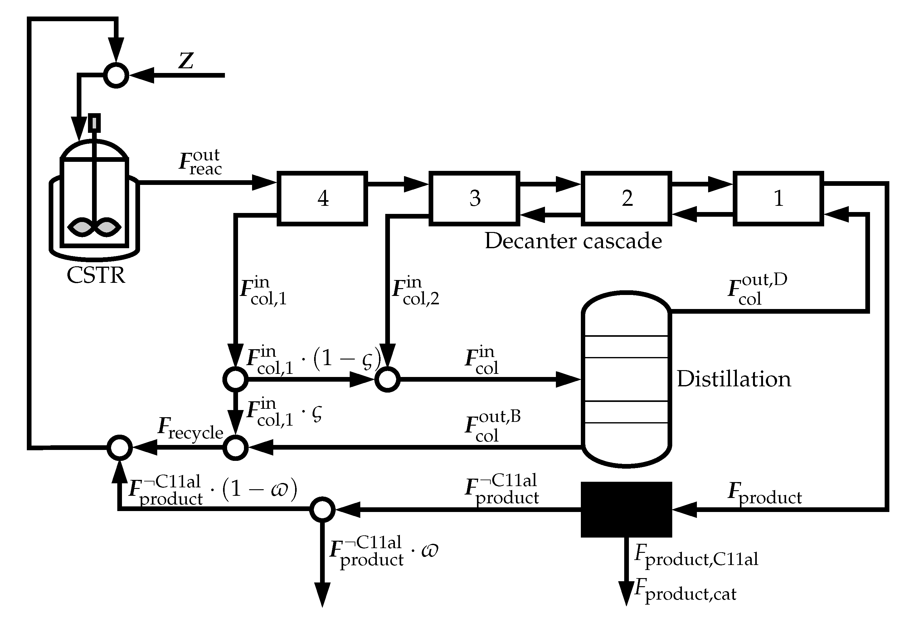
The reactor inlet F reac in is composed of three elements. The first of these is the feed stream, Z , which contains the make-up streams for the catalyst, the solvents, and the reactants. The second is the recycle stream, F recycle , coming from the decanter cascade, which recycles the polar solvent (thereby the catalyst), unused reactants, and some of the products. The final stream is the recycle coming from the black box, F product ¬ C 11 al , minus the purged stream.

2.2.2. Downstream Processing

The reactor outlet, F reac out , is fed into the downstream section consisting of four decanters and a distillation column.
The distillation column is required to recover the extraction solvent. It is assumed to be operated at a pressure of 60 mbar, with a linear pressure drop of 30 mbar along the column. The requirement of the column is that it recovers all of the circulated extraction solvent F ( p s o l ) at the top. Instead of a rigorous distillation column model, a separately calculated surrogate function is employed for each investigated polar solvent p s o l . The procedure to obtain the surrogate function can be split into two parts.
First, the relative volatilities α are calculated. An ensemble of 810 distillation columns with a different number of stages, reflux, and reboil ratios were simulated. Each distillation column is assumed to have constant molar flows, a constant molar overflow, and a total condenser. Furthermore, each is assumed to behave ideally, thus the gas phase is described by Dalton’s law P vap = χ · P and the liquid phase is described by Raoult’s law P vap = Υ · P vap * , where χ and Υ are the liquid and vapor mole fractions, respectively. For the calculation of the vapor pressures the vapor pressure correlation
log 10 P vap * = a 0 + a 1 · T 1 + a 2 · log 10 ( T ) + a 3 · T + a 4 · T 2
is used, with T in K and P vap * in mmHg. The parameters a i can be found in Table A1. Using these 810 simulations, mean temperatures for the top of the column, T ¯ D , and the bottom of the column, T ¯ B , can be calculated. These mean temperatures are used to calculate the relative volatilities using Equation (5) and
α i = P ¯ vap , B , i * P ¯ vap , B , HK * · P ¯ vap , D , i * P ¯ vap , D , HK * ,
where HK denotes the highest boiling component, i.e., C11al. The obtained values for α can be found in Table A3.
The optimal costs for the distillation are calculated using the constant α . Global optimizations using BARON [53], with a Fenske–Underwood–Gilliland (FUG) shortcut model [54], were conducted with 1000 varied feeds for each solvent. For these global optimizations the constraints are as follows:
  • DMF: 99% purity of DMF in the distillate
  • DSUC: 99% purity of DSUC + C10en in the distillate
  • THPO: 99% purity of THPO in the distillate
The varied purity requirements for the different polar solvent candidates are necessary because of their different separation properties. These properties will be explained later.
The total annualized costs (TAC) in $ / a for the distillation column are calculated with a lumped cost function [55]
J col = κ 1 · V col + κ 2 · ( l col + κ 3 ) κ 4 · ( V col · κ 5 ) κ 6 + κ 7 · ( l col + κ 8 ) κ 9 · ( V col · κ 10 ) κ 11 ,
using the parameters from Table A2, where V col is the vapor flow rate and l col is the length of the column.
The values of J col are used for a polynomial regression of the costs with respect to the circulated extraction solvent stream F ( p s o l ) and the recovery rate r e c = F ( p s o l ) / F col , p s o l in ,
T A C col = λ p s o l , 1 + λ p s o l , 2 · F ( p s o l ) + λ p s o l , 3 · r e c + λ p s o l , 4 · F ( p s o l ) 2 + λ p s o l , 5 · r e c 2 ,
with parameters λ given in Table A2. Equation (8) is used as a surrogate for the distillation column.
The number of decanters is chosen because it was cost optimal in a previous study [56]. Following the results of [56] once again, the decanters are operated at a fixed temperature of 298.15 K. The decrease in temperature compared to the reaction conditions leads to a liquid–liquid phase split. The mass balances are defined as follows,
F dec , n in = V 2 + F col out , D , for n = 1 , L n 1 + V n + 1 , for 1 < n < n max , F reac out , for n = n max ,
where the decanters are numbered from right to left, i.e., [ n max , , 1 ] . The upper outlet of the decanters V is the less polar, product-rich phase with composition y and the lower outlet of the decanters L is the more polar, catalyst-rich phase with composition x .
The boiling points of the three solvents vary, with DMF being the easiest to separate and DSUC being the hardest to separate (see the relative volatilities α in Table A3). Therefore, the separation properties of the three solvents regarding distillation vary. With DMF and THPO, it is possible to solely recover the solvent in the distillate stream. With DSUC, C10en becomes the component with the highest relative volatility. Therefore, we assume that all of the C10en contained in the column feed will leave through the distillate.
Because the components contained in the distillate flow differ depending on the separation properties of the solvents, the value of F col , i out , D needs to be calculated as
F col , i out , D = β i ( p s o l ) F col , i in ,
because the column itself is replaced by the aforementioned surrogate function in Equation (8). Here, β ( p s o l ) is introduced as a vector of split factors for ( p s o l , C12an, C10en, C11al, cat) to capture the different separation behaviors of the mixture with the respective solvent:
β ( DMF ) = ( ς p s o l , 0 , 0 , 0 , 0 ) ,
β ( DSUC ) = ( ς p s o l , 0 , 1 , 0 , 0 ) ,
β ( THPO ) = ( ς p s o l , 0 , 0 , 0 , 0 ) .
Here, ς p s o l is used to make sure that only the circulated extraction solvent stream F ( p s o l ) leaves the distillation column through the distillate.
Note that the fourth and the third decanter are only connected through the less polar flow of the fourth decanter. By doing this, the extraction solvent stream of the cascade bypasses the fourth decanter, allowing for an additional degree of freedom. The molar flow entering the column, F col in , is composed of the more polar phase of the third decanter, F col , 2 in = L 3 , and a fraction of the more polar phase of the fourth decanter, F col , 1 in = L 4 ,
F col in = L 4 ( 1 ς ) + L 3 .
That fraction is determined by the split factor ς [ 0 , 1 ] . A large split factor leads to a smaller flow into the column. However, the composition of the mixture at the bottom of the column, and hence the temperature, also depends on the split factor. The literature suggests that the aldehyde will react with itself to the unwanted side product aldol at temperatures above 403.15 K [57]. Therefore, the temperature at the bottom of the column is restricted to 388.15 K, the same temperature as inside the reactor, which should be safe. The split factor ς can be used by the optimizer to achieve this temperature.
The catalyst inside the decanter cascade is described by the catalyst mass balance
F reac , cat out = L n max cat + L n max 1 cat + V 1 cat ,
where L cat is the catalyst in the more polar phase and V cat is the catalyst in the less polar phase. The partitioning of the catalyst between the two phases is calculated with
log 10 P yx , n = log 10 V n cat L n V n L n cat ,
where log 10 P yx , n is the logarithmic partition coefficient for stage n.
The activity coefficients γ for the LLE are described by a modified UNIFAC (Dortmund) [58] implementation. The corresponding LLE conditions,
x i γ i ( I ) y i γ i ( I I ) = 0 ,
are solved with a residuum less than 1 × 10⁻⁹. For each of the LLE points, the partition coefficients P y x for the catalyst/ligand is calculated with COSMOtherm [47], because the size of the catalyst/ligand complex prohibits the use of group contribution methods such as UNIFAC [59]. To determine the composition of the two liquid phases and the catalyst distribution, a surrogate model f ^ is employed,
[ x i , n , y i , n , log 10 P yx , n ] = f ^ ( t 1 , n , t 2 , n ) ,
where ( t 1 , n , t 2 , n ) [ 0 , 1 ] 2 is a parameterization of the binodal curve. To generate the input/output data for fitting the surrogate model, a parameter continuation [60] in the orthogonal direction of the tie lines of the LLE is used.
The surrogate has a two-dimensional input space and a nine-dimensional output space. It consists of a second-degree polynomial and an ANN with a single hidden layer fit to the residuals of the polynomial. The ANN is generated with the “train” command of MATLABs deep learning toolbox. A more thorough description of the algorithm used to generate the surrogate is not the scope of this article and can be found in another publication of the authors in the present special issue of Processes [61].
A previous optimization study yielded that the catalyst recovery plays an important role for the overall process cost [56]. Therefore, the accuracy of the employed surrogate with regard to the partition coefficient P yx is of high importance. The maximum errors of the three surrogate models for log 10 P yx = f p s o l P yx ( t 1 , t 2 ) at the sample points are:
a δ ¯ p s o l = max f p s o l P yx ( t 1 , t 2 ) f ^ p s o l P yx ( t 1 , t 2 ) , a δ ¯ p s o l = min f p s o l P yx ( t 1 , t 2 ) f ^ p s o l P yx ( t 1 , t 2 ) , δ ¯ DMF a = 0.001087 , δ ¯ DMF a = 0.000684 , δ ¯ DSUC = 0.000524 , δ ¯ DSUC = 0.001201 , δ ¯ THPO = 0.002302 , δ ¯ THPO = 0.001656 .

2.2.3. Black Box

The process considered in this work is the first step in an attempt to optimize the hydroformylation simultaneously with a reductive amination (RA) step. In the RA the product of the hydroformylation (C11al) and diethylamine are used to generate the corresponding amine, which is a valuable product used as a building block for agrochemical and pharmaceutical chemicals as well as surfactants, coatings, and lubricants. Although we currently do not have a rigorous process model for the reductive amination, the underlying conditions influencing the hydroformylation are known from the design specifications for the reductive amination process. Therefore, it is modeled as a black box with some simplifying assumptions. We assume that the aldehyde is separated from the other species in the cause of the RA and that the other species are recycled to the hydroformylation process. The catalyst present in the product stream is assumed to be lost during this separation process.

2.2.4. Overall Process

In order to connect the process parts described above efficiently, some further considerations had to be taken into account.
Eleven species are necessary to describe the reactions and interactions inside the reactor, see Table 1. Not every species important for the reaction plays a role in the extraction cascade. The isomerized C10en and C11al can be seen to behave identically to their respective non-isomerized counterparts during the extraction. Therefore, the isomerized and non-isomerized species are treated as if they were a single species in the extraction, thereby reducing the number of species by two. Furthermore, C10an and C12an can both be used as a non-polar solvent for the extraction, and are therefore combined into one non-polar solvent stream assumed to behave like C12an since the amount of C12an is clearly higher. Furthermore, it is also assumed that only the liquid phase of the reactor goes into the extraction cascade. With these assumptions, the number of species in the extraction cascade can be reduced to five. The reactor outlet F reac out then consists of the following species,
F reac out = p s o l C 12 an C 10 en C 11 al cat ,
where p s o l [ DMF , DSUC , THPO ] is one of the investigated solvents and cat is the catalyst/ligand complex.
To keep the whole model consistent, the ratios of the combined species in the extraction cascade are assumed to be identical for the reactor outlet and the recycle streams, i.e., n-/iso-ratios and C10an/C12an ratio.

2.3. Process Optimization

The process optimizations in this work are mixed integer nonlinear programs (MINLPs) of the following form:
min x ˜ J ( x ˜ ) , s . t . h ( x ˜ ) = 0 , g ( x ˜ ) 0 , x ˜ G , G R n , x ˜ i Z , Z Z , for all i I ,
where J ( x ˜ ) is the objective function, h ( x ˜ ) are the equality constraints, such as mass balances, and g ( x ˜ ) are the inequality constraints, such as purity requirements. The variables x ˜ include the degrees of freedom, of these variables x ˜ i with i I have to fulfill integrality restrictions.
The degrees of freedom are the feed flows Z of the reactant, the catalyst, and the solvents, the hold-up time in the reactor, characterized by the reactor volume, V reac [ 2.1853 , 4000 ] m 3 , the reactor temperature, T r [ 368.15 , 388.15 ] K, and pressure, P r [ 10 , 20 ] bar, the amount of extraction solvent used in the extraction cascade, F ( p s o l ) [ 7 , 90 ] mol/s, the split factor ς [ 0 , 1 ] , and the purge ϖ [ 0.0001 , 0.01 ] . Note, that the model would yield an NLP without the piecewise linear approximation of the activation function of the ANN describing the gas solubility in the reactor. This model reformulation yields an MINLP but is beneficial for reducing the computational burden [34].
Besides the mass balances, there is the overall process requirement of a product yield of 2 mol/s C11al, which roughly translates into 6500 metric tons of product per year.
The objective function is defined as
J = T A C dec + T A C col + T A C cat + T A C reac ,
T A C dec = θ 1 n i η i F dec , n , i in θ 2 ,
T A C col = λ p s o l , 1 + λ p s o l , 2 · F ( p s o l ) + λ p s o l , 3 · r e c + λ p s o l , 4 · F ( p s o l ) 2 + λ p s o l , 5 · r e c 2 ,
T A C cat = θ 3 V 1 cat ,
T A C reac = θ 4 m cat + θ 5 V reac θ 6 + θ 7 i θ 8 , i Z i 2 θ 8 , C 10 en ,
where Equation (23) describes the costs for the decanters [35], Equation (24) describes the costs for the extraction solvent column, Equation (25) describes the costs for the catalyst make-up, and Equation (26) describes the costs for the reactor [35], including the reactant stream and make-up streams for the solvents. The parameters θ , η , and λ can be found in Table A2.
The process optimizations are implemented as MINLPs and solved using the GAMS 26.1.0 framework with the multi-start heuristic of the deterministic global optimization software BARON 18.11.12., Cplex 12.8.0 is used as an LP/MIP subsolver, and CONOPT 4.09 is utilized as an NLP subsolver. The calculations are carried out on a Linux PC with 3.40 GHz Intel Core i7-6700 CPU and 16 GB memory.

3. Results

3.1. Process Optimization for Each Candidate Solvent

This section will present the process optimization results for each of the solvent candidates. The results were obtained by an optimization using BARONs multi-start heuristic with 140,000 starting points.
Some important molar flow rates can be found in Figure 2. For each of the three solvent candidates, a simplified version of the flowsheet is depicted. The highlighted boxes containing the molar flow rates point to the respective points in the flowsheet where these values are obtained. Additionally, the degrees of freedom missing from Figure 2 can be found in Table 2.

3.1.1. Dimethylformamide (DMF)

The first of the three solvent candidates is the benchmark, DMF. It is well known to be ideally suitable for TMS in conjunction with an alkane. The catalyst recovery of 99.99992% in the extraction cascade is very good, therefore the catalyst concentration in the reactor can be high. A high catalyst concentration leads to faster reaction rates and thus the residence time can be low. The main parameter for the residence time is the reactor volume, V reac , which can be relatively small and with that the investment costs for the reactor are reduced. For the same reason, the reactor pressure, P r , and temperature, T r , are set to their maximum values to achieve fast reaction rates.
The extraction solvent stream in the extraction cascade can be relatively small because DMF has good selectivity for the catalyst. The split factor, ς , is set to zero, meaning that all of the stream that could be bypassed directly into the recycle, F col in , 1 , is let into the column. The first reason is that F col in , 2 , DMF is close to the value of the circulated extraction solvent stream F ( DMF ) . Therefore, there would be only a little of the polar solvent left at the bottom of the distillation column, leading to a temperature that would be too high, and the distillation would be quite expensive because of the high recovery rate. The second reason is that F col in , 1 is composed of 92.91% DMF and the combined flow is composed of 92.97% DMF, which is quite close to the purity requirement at the top of the column. Therefore, the recovery rate of the polar solvent at the top of the column becomes smaller and the column becomes cheaper, though its diameter has to be a little larger because of the increased input stream.
A small fraction of the recycled product stream, ϖ , needs to be purged. The purge is the only sink for the side product C10an. Therefore, the purge is necessary, although it is quite expensive because of the purged reactant and solvents. The purged solvents need to be reintroduced through the feed stream, together with the amount of catalyst lost in the product stream and the necessary reactant.
The total annualized costs are 1,934,522 $/a.
We assume that the real value for the partition coefficient P yx , DMF lies within the interval [ f ^ ( t 1 , t 2 ) + δ ¯ DMF , f ^ ( t 1 , t 2 ) + δ ¯ DMF ] . To account for the surrogate model errors listed in Equation (19), an additional optimization with P yx = f ^ ( t 1 , t 2 ) + δ ¯ is conducted for each solvent candidate. By adding the maximum error at the sampling points of the surrogate, the catalyst distribution changes and more catalyst will be lost. The worst case annualized costs with regard to the approximation quality of the surrogate are 1,939,897 $/a.

3.1.2. Dimethyl Succinate (DSUC)

The catalyst recovery of 99.9972% in the extraction cascade achieved with DSUC is smaller than in the previous benchmark case. Therefore, the catalyst concentration has to be smaller in the reactor and consequently, the residence time has to be larger. The reactor volume has to be 12.6 times the size of the benchmark case, and the investment costs for the reactor are also higher. The reactor pressure, P r , and temperature, T r , are set to their maximum values to achieve fast reaction rates.
The extraction solvent stream has to be 1.75 times that of the benchmark case since DSUC is not as selective with regard to the catalyst as DMF is. Therefore, the distillation column and the decanters have to be larger, increasing the investment costs. Furthermore, the operating costs for the distillation column are increased because more solvent needs to be vaporized. In contrast to the benchmark case, F col in , 1 only contains 80.54% DSUC. However, if both streams, F col in , 1 and F col in , 2 , are summed up the percentage of DSUC remains constant and the overall flux is larger, which reduces the costs due to the reduced recovery rate. Note, that the distillate is now composed of the extraction solvent and the C10en entering the column.
Again, a small fraction of the recycled product stream needs to be purged to remove C10an. In this test case, the overall molar flow rates are higher than in the previous benchmark case. DSUC drags more of the product, C11al, into the recycle. Therefore, to achieve the required amount of C11al in the product flow, the inlet flow of C11al into the extraction cascade needs to be doubled compared to the benchmark case. Furthermore, more solvent is necessary due to the fixed ratio of solvents to the other species in the reactor. Additionally, as there is more of the reactant in the reactor, more of the side products are generated. Consequently, the purge needs to be larger.
The total annualized costs are 6,154,228 $/a, 3.18 times the costs of the benchmark case.
The worst case annualized costs with regard to the approximation quality of the surrogate are 6,177,063 $/a.

3.1.3. Tetrahydropyranone (THPO)

The catalyst recovery in the extraction cascade is 99.99993% and thus even better than in the benchmark case. For that reason, the catalyst concentration in the reactor can be higher and therefore the reactor volume can be smaller. Again, the reactor pressure, P r , and temperature, T r , are set to their maximum values to achieve fast reaction rates.
The extraction solvent stream is a bit smaller than that of the benchmark case. Because the composition of F col , 1 in is also similar to that of the benchmark case, the same choice of the split factor is used by the optimizer and the entire stream is fed to the column to make the distillation cheaper.
The purge that removes the side-product C10an is a little larger than in the benchmark case.
Interestingly, the total annualized costs for the process with THPO as polar solvent are 1,748,021 $/a, 0.9036 times the costs of the benchmark. This is mainly due to the increased catalyst recovery. The catalyst make-up is the most expensive part of the whole process.
The worst case annualized costs with regard to the approximation quality of the surrogate are 1,758,083 $/a.

4. Conclusions

In this work, an approach for an integrated process and solvent design was presented. In our approach, unsuitable solvent candidates from known databases are eliminated during a screening procedure and a rigorous process optimization is conducted for the remaining solvent candidates.
DSUC and THPO have been identified by the screening procedure as ecologically benign solvent candidates for a hydroformylation process employing a TMS. They have been compared with the well known and developmental toxic benchmark solvent DMF.
The optimization results show that the selectivity of the solvent with respect to the catalyst and the product is of high importance. DSUC has a low selectivity for the catalyst and thus its use leads to an increased catalyst loss. This catalyst loss is compensated by the optimizer with a lower catalyst concentration in the reactor and thus a higher residence time. Furthermore, DSUC dissolves much of the product, leading to a high product recycle and consequently to higher overall fluxes and larger facilities. This renders DSUC unsuitable because of the greatly increased costs.
On the other hand, THPO has shown that it can recover the catalyst even better than DMF under the assumed operating conditions. Though it is slightly harder to separate from the other species by distillation than DMF, the use of THPO reduces the total annualized costs by 9.64%. This leads to the conclusion that the ability of the polar solvent to recover the catalyst while leaving the product in the less polar phase is of utmost importance.
Though the small savings lie within the economic uncertainties of the objective function, we have shown that a process with a well-established toxic solvent can be replaced by a process with an ecologically benign solvent with similar costs. A quantitative evaluation also depends on model accuracy, in particular the accuracy of the partition coefficient of the catalyst in the different solvent systems. In any case, experimental validation is necessary and will be part of future work.
Our present work was limited to already known solvent candidates from databases. To overcome this limitation, further research will be concerned with computer-aided molecular design approaches in Conjunction With Process Optimization.

Author Contributions

Conceptualization, T.K., C.K.; methodology, T.K., C.K., S.L., K.M.; software, T.K., C.K. and S.L.; validation, T.K., C.K.; formal analysis, T.K. and S.L.; investigation, T.K. and S.L.; data curation, S.L.; writing–original draft preparation, T.K. and S.L.; writing–review and editing, T.K., C.K., S.L., K.M., A.K.; visualization, T.K.; supervision, K.S. and A.K.; Funding acquisition, K.S. and A.K. Please turn to the CRediT taxonomy for the term explanation.

Funding

This research was funded by DFG grant number TRR 63.

Acknowledgments

This work is part of the Collaborative Research Center “Integrated Chemical Processes in Liquid Multiphase Systems - InPROMPT”. Financial support by the Deutsche Forschungsgemeinschaft (DFG) is gratefully acknowledged through SFB/TRR 63.

Conflicts of Interest

The authors declare no conflict of interest.

Nomenclature

Vector-valued:
a i vapor pressure parameters
α relative volatilities
T ¯ mean temperature
χ liquid mole fraction
γ vector of activity coefficients
κ cost function parameters
λ column cost parameters
ν stoichiometric coefficients
Υ vapor mole fraction
c concentration
F molar flow rate
g inequality constraints
h equality constraints
K reaction rate parameters
k reaction rate constants
L molar flow rate, phase I
P vap vapor pressure
r reaction rates
V molar flow rate, phase II
x liquid composition, phase I
y liquid composition, phase II
Z molar feed flow rate
Real-valued:
ϖ purge fraction
ς split fraction
i , n count variable
J ( x ) objective function
l col column length
Ppressure
p s o l polar solvent
Ttemperature
T A C total annualized cost
V col vapor flow rate, column
V reac reactor volume
Abbreviations:
ANNArtificial Neural Network
CAMDComputer-Aided Molecular Design
COSMO-RSContinuum Solvation Model for Realistic Solvents
DMFDimethylformamide
DSUCDimethylsuccinate
EHSEnvironment, health, and safety
EOSEquation Of State
FUGFenske–Underwood–Gilliland
InPROMPTIntegrated chemical processes in liquid multiphase system
LLELiquid–Liquid Equilibrium
MINLPMixed-Integer Non-Linear Program
MOOMulti-Objective Optimization
PC-SAFTPerturbed-Chain Statistical Associating Fluid Theory
RAReductive Amination
SVHCSubstance of Very High Concern
THPOTetrahydropyranone
TMSThermomorphic Multiphase System
UNIFACUniversal Quasichemical Functional Group Activity Coefficients

Appendix A

This appendix includes thermodynamic and physical species data, as well as cost function parameters.
Table A1. Vapor pressure parameters ( 10 a 0 + a 1 T 1 + a 2 log 10 ( T ) + a 3 T + a 4 T 2 ) [mmHg]. Vapor pressure correlations for DSUC and THPO are fitted with the method presented in [62], the other values are taken from [63].
a 0 a 1 a 2 a 3 a 4
DMF−47.9857 2.385 × 10 3 28.8 5.8596 × 10 2 3.1386 × 10 5
DSUC117.8014 6.3944 × 10 3 −42.5731 3.0869 × 10 2 9.2995 × 10 6
THPO74.2227 4.2846 × 10 3 −25.9627 1.8373 × 10 2 5.4143 × 10 6
C10en2.2678 3.12 × 10 3 5.43 2.01 × 10 2 1.12 × 10 5
C12an−8.5899 3.5241 × 10 3 10.806 2.8161 × 10 2 1.4267 × 10 5
C11al−31.8129 3.14 × 10 3 20.4 3.73 × 10 2 1.75 × 10 5
Table A2. Cost function parameters for each investigated solvent.
ParameterDMFDSUCTHPO
κ 1 17 , 764 15,07117,783
κ 2 2463.6 2988.6 2202.3
κ 3 7.2 7.2 7.2
κ 4 0.81 0.81 0.81
κ 5 111
κ 6 0.525 0.525 0.525
κ 7 155.4357 202.9541 133.1394
κ 8 0.8 0.8 0.8
κ 9 0.97 0.97 0.97
κ 10 111
κ 11 0.725 0.725 0.725
λ 1 64,191168,83351,628
λ 2 20,63819,65620,695
λ 3 −56,984−182,134−53,368
λ 4 −9.6219−4.2671−12.5046
λ 5 98,841439,84071,678
η C 10 en 0.21041 × 10 3 0.21041 × 10 3 0.21041 × 10 3
η p s o l 0.07915 × 10 3 0.12395 × 10 3 0.08491 × 10 3
η C 12 an 0.233642 × 10 3 0.233642 × 10 3 0.233642 × 10 3
η C 11 al 0.195184 × 10 3 0.195184 × 10 3 0.195184 × 10 3
θ 1 504,155504,155504,155
θ 2 0.5866670.5866670.586667
θ 3 2.9661 × 10 12 2.9661 × 10 12 2.9661 × 10 12
θ 4 85,15085,15085,150
θ 5 17,248.4217,248.4217,248.42
θ 6 0.620.620.62
θ 7 2.8512 × 10 7 2.8512 × 10 7 2.8512 × 10 7
θ 8 , C 10 en 0.6610.6610.661
θ 8 , p s o l 0.07310.07310.0731
θ 8 , C 12 an 0.07140.07140.0714
Table A3. Relative volatilities.
α DMF α DMS α THPO
DMF31.9942[-][-]
DMS[-]4.0208[-]
THPO[-][-]22.4438
C12an3.13072.77663.0696
C10en16.866911.730815.8739
C11al111

References

  1. Anastas, P.T.; Warner, J.C. Green Chemistry: Theory and Practice; Oxford University Press: Oxford, UK, 1998. [Google Scholar]
  2. Linthorst, J.A. An overview: Origins and development of green chemistry. Found. Chem. 2010, 12, 55–68. [Google Scholar] [CrossRef]
  3. Hoffenson, S.; Dagman, A.; Söderberg, R. Re-engineering Manufacturing for Sustainability; Chapter A Multi-Objective Tolerance Optimization Approach for Economic, Ecological, and Social Sustainability; Springer: Berlin, Germany, 2013; pp. 729–734. [Google Scholar]
  4. Elkington, J. Cannibals with Forks: The Triple Bottom Line of 21st Century Business; New Society Publishers: Gabriola Island, BC, Canada, 1998. [Google Scholar]
  5. Lundberg, I.; Lidén, C. Handbook of Hazardous Materials; chapter Industrial Solvents; Academic Press: San Diego, CA, USA, 1993; pp. 387–397. [Google Scholar] [CrossRef]
  6. Joback, K.G.; Reid, R.C. Estimation of Pure-Component Properties from Group-Contributions. Chem. Eng. Commun. 1987, 56, 233–243. [Google Scholar] [CrossRef]
  7. Burger, J.; Papaioannou, V.; Gopinath, S.; Jackson, G.; Galindo, A.; Adjiman, C.S. A hierarchical method to integrated solvent and process design of physical CO2 absorption using the SAFT-γ Mie approach. AIChE J. 2015, 61, 3249–3269. [Google Scholar] [CrossRef]
  8. Papadopoulos, A.I.; Stijepovic, M.; Linke, P. On the systematic design and selection of optimal working fluids for Organic Rankine Cycles. Appl. Therm. Eng. 2010, 30, 760–769. [Google Scholar] [CrossRef]
  9. Zhou, T.; Song, Z.; Zhang, X.; Gani, R.; Sundmacher, K. Optimal Solvent Design for Extractive Distillation Processes: A Multiobjective Optimization-Based Hierarchical Framework. Ind. Eng. Chem. Res. 2019, 58, 5777–5786. [Google Scholar] [CrossRef]
  10. Karunanithi, A.T.; Achenie, L.E.K.; Gani, R. A New Decomposition-Based Computer-Aided Molecular/Mixture Design Methodology for the Design of Optimal Solvents and Solvent Mixtures. Ind. Eng. Chem. Res. 2005, 44, 4785–4797. [Google Scholar] [CrossRef]
  11. Cignitti, S.; Mansouri, S.S.; Woodley, J.M.; Abildskov, J. Systematic Optimization-Based Integrated Chemical Product–Process Design Framework. Ind. Eng. Chem. Res. 2017, 57, 677–688. [Google Scholar] [CrossRef]
  12. Eden, M.; Jøorgensen, S.; Gani, R.; El-Halwagi, M. A novel framework for simultaneous separation process and product design. Chem. Eng. Process. 2004, 43, 595–608. [Google Scholar] [CrossRef]
  13. Kossack, S.; Kraemer, K.; Gani, R.; Marquardt, W. A systematic synthesis framework for extractive distillation processes. Chem. Eng. Res. Des. 2008, 86, 781–792. [Google Scholar] [CrossRef]
  14. Gopinath, S.; Jackson, G.; Galindo, A.; Adjiman, C.S. Outer approximation algorithm with physical domain reduction for computer-aided molecular and separation process design. AIChE J. 2016, 62, 3484–3504. [Google Scholar] [CrossRef]
  15. First, E.L.; Hasan, M.M.F.; Floudas, C.A. Discovery of novel zeolites for natural gas purification through combined material screening and process optimization. AIChE J. 2014, 60, 1767–1785. [Google Scholar] [CrossRef]
  16. Jens, C.M.; Nowakowski, K.; Scheffczyk, J.; Leonhard, K.; Bardow, A. CO from CO 2 and fluctuating renewable energy via formic-acid derivatives. Green Chem. 2016, 18, 5621–5629. [Google Scholar] [CrossRef]
  17. Zhou, T.; Zhou, Y.; Sundmacher, K. A hybrid stochastic–deterministic optimization approach for integrated solvent and process design. Chem. Eng. Sci. 2017, 159, 207–216. [Google Scholar] [CrossRef]
  18. Papadopoulos, A.I.; Linke, P. Multiobjective molecular design for integrated process-solvent systems synthesis. AIChE J. 2005, 52, 1057–1070. [Google Scholar] [CrossRef]
  19. Limleamthong, P.; Gonzalez-Miquel, M.; Papadokonstantakis, S.; Papadopoulos, A.I.; Seferlis, P.; Guillén-Gosálbez, G. Multi-criteria screening of chemicals considering thermodynamic and life cycle assessment metrics via data envelopment analysis: Application to CO2 capture. Green Chemistry 2016, 18, 6468–6481. [Google Scholar] [CrossRef]
  20. Ten, J.Y.; Hassim, M.H.; Ng, D.K.S.; Chemmangattuvalappil, N.G. A molecular design methodology by the simultaneous optimisation of performance, safety and health aspects. Chem. Eng. Sci. 2017, 159, 140–153. [Google Scholar] [CrossRef]
  21. Scheffczyk, J.; Redepenning, C.; Jens, C.M.; Winter, B.; Leonhard, K.; Marquardt, W.; Bardow, A. Massive, automated solvent screening for minimum energy demand in hybrid extraction–distillation using COSMO-RS. Chem. Eng. Res. Des. 2016, 115, 433–442. [Google Scholar] [CrossRef]
  22. Scheffczyk, J.; Schäfer, P.; Fleitmann, L.; Thien, J.; Redepenning, C.; Leonhard, K.; Marquardt, W.; Bardow, A. COSMO-CAMPD: A framework for integrated design of molecules and processes based on COSMO-RS. Mol. Syst. Des. Eng. 2018, 3, 645–657. [Google Scholar] [CrossRef]
  23. Scheffczyk, J.; Schäfer, P.; Jens, C.M.; Leonhard, K.; Bardow, A. Integrated process and solvent design using COSMO-RS for the production of CO from CO2 and H2. In Computer Aided Chemical Engineering; Elsevier: Amsterdam, The Netherlands, 2017; Volume 40, pp. 1765–1770. [Google Scholar] [CrossRef]
  24. Fleitmann, L.; Scheffczyk, J.; Schäfer, P.; Jens, C.M.; Leonhard, K.; Bardow, A. Integrated Design of Solvents in Hybrid Reaction-Separation Processes Using COSMO-RS. Chem. Eng. Trans. 2018, 2018, 559–564. [Google Scholar] [CrossRef]
  25. Bardow, A.; Steur, K.; Gross, J. Continuous-Molecular Targeting for Integrated Solvent and Process Design. Ind. Eng. Chem. Res. 2010, 49, 2834–2840. [Google Scholar] [CrossRef]
  26. Stavrou, M.; Lampe, M.; Bardow, A.; Gross, J. Continuous Molecular Targeting–Computer-Aided Molecular Design (CoMT–CAMD) for Simultaneous Process and Solvent Design for CO2 Capture. Ind. Eng. Chem. Res. 2014, 53, 18029–18041. [Google Scholar] [CrossRef]
  27. Wang, J.; Lakerveld, R. Integrated solvent and process design for continuous crystallization and solvent recycling using PC-SAFT. AIChE J. 2018, 64, 1205–1216. [Google Scholar] [CrossRef]
  28. Lampe, M.; Stavrou, M.; Schilling, J.; Sauer, E.; Gross, J.; Bardow, A. Computer-aided molecular design in the continuous-molecular targeting framework using group-contribution PC-SAFT. Comput. Chem. Eng. 2015, 81, 278–287. [Google Scholar] [CrossRef]
  29. McBride, K.; Linke, S.; Xu, S.; Sundmacher, K. Computer Aided Design of Green Thermomorphic Solvent Systems for Homogeneous Catalyst Recovery. In Proceedings of the 13th International Symposium on Process Systems Engineering (PSE 2018), San Diego, CA, USA, 1–5 July 2018; pp. 1783–1788. [Google Scholar] [CrossRef]
  30. Bianga, J.; Künnemann, K.; Gaide, T.; Vorholt, A.J.; Seidensticker, T.; Dreimann, J.; Vogt, D. Thermomorphic Multiphase Systems: Switchable Solvent Mixtures for the Recovery of Homogeneous Catalysts in Batch and Flow Processes. Chem. Eur. J. 2019, 25, 1–24. [Google Scholar] [CrossRef] [PubMed]
  31. Schäfer, E.; Brunsch, Y.; Sadowski, G.; Behr, A. Hydroformylation of 1-Dodecene in the Thermomorphic Solvent System Dimethylformamide/Decane. Phase Behavior-Reaction Performance-Catalyst Recycling. Ind. Eng. Chem. Res. 2012, 51, 10296–10306. [Google Scholar] [CrossRef]
  32. Kiedorf, G.; Hoang, D.; Müller, A.; Jörke, A.; Markert, J.; Arellano-Garcia, H.; Seidel-Morgenstern, A.; Hamel, C. Kinetics of 1-dodecene hydroformylation in a thermomorphic solvent system using a rhodium-biphephos catalyst. Chem. Eng. Sci. 2014, 115, 31–48. [Google Scholar] [CrossRef]
  33. Hentschel, B.; Kiedorf, G.; Gerlach, M.; Hamel, C.; Seidel-Morgenstern, A.; Freund, H.; Sundmacher, K. Model-Based Identification and Experimental Validation of the Optimal Reaction Route for the Hydroformylation of 1-Dodecene. Ind. Eng. Chem. Res. 2015, 54, 1755–1765. [Google Scholar] [CrossRef]
  34. Keßler, T.; Mertens, N.; Kunde, C.; Nentwich, C.; Michaels, D.; Engell, S.; Kienle, A. Efficient global optimization of a novel hydroformylation process. In 27th European Symposium on Computer Aided Process Engineering; Espuña, A., Graells, M., Puigjaner, L., Eds.; Elsevier: Amsterdam, The Netherlands, 2017; Volume 40, pp. 2113–2118. [Google Scholar] [CrossRef]
  35. McBride, K.; Sundmacher, K. Data Driven Conceptual Process Design for the Hydroformylation of 1-Dodecene in a Thermomorphic Solvent System. Ind. Eng. Chem. Res. 2015, 54, 6761–6771. [Google Scholar] [CrossRef]
  36. Nentwich, C.; Engell, S. Application of surrogate models for the optimization and design of chemical processes. In Proceedings of the 2016 International Joint Conference on Neural Networks (IJCNN), Vancouver, BC, Canada, 24–29 July 2016; pp. 1291–1296. [Google Scholar] [CrossRef]
  37. Dreimann, J.M.; Hoffmann, F.; Skiborowski, M.; Behr, A.; Vorholt, A.J. Merging Thermomorphic Solvent Systems and Organic Solvent Nanofiltration for Hybrid Catalyst Recovery in a Hydroformylation Process. Ind. Eng. Chem. Res. 2017, 56. [Google Scholar] [CrossRef]
  38. Hernández, R.; Engell, S. Modelling and iterative real-time optimization of a homogeneously catalyzed hydroformylation process. Comput. Aided Chem. Eng. 2016, 38, 1–6. [Google Scholar] [CrossRef]
  39. Illner, M.; Müller, D.; Esche, E.; Pogrzeba, T.; Schmidt, M.; Schomäcker, R.; Wozny, G.; Repke, J.U. Hydroformylation in Microemulsions: Proof of Concept in a Miniplant. Ind. Eng. Chem. Res. 2016, 55. [Google Scholar] [CrossRef]
  40. Müller, D.; Illner, M.; Esche, E.; Pogrzeba, T.; Schmidt, M.; Schomäcker, R.; Biegler, L.T.; Wozny, G.; Repke, J.U. Dynamic real-time optimization under uncertainty of a hydroformylation mini-plant. Comput. Chem. Eng. 2017, 106, 836–848. [Google Scholar] [CrossRef]
  41. Kraume, M. Integrierte chemische Prozesse in flüssigen Mehrphasensystemen. Chemie Ingenieur Technik 2013, 85, 1499–1511. [Google Scholar] [CrossRef]
  42. Behr, A.; Vorholt, A.J. Hydroformylation and Related Reactions of Renewable Resources; Springer: Berlin/Heidelberg, Germany, 2012; pp. 103–127. [Google Scholar] [CrossRef]
  43. Behr, A.; Obst, D.; Westfechtel, A. Isomerizing hydroformylation of fatty acid esters: Formation of ω-aldehydes. Eur. J. Lipid Sci. Technol. 2005, 107, 213–219. [Google Scholar] [CrossRef]
  44. Fail, P.A.; George, J.D.; Grizzle, T.B.; Heindel, J.J. Formamide and Dimethylformamide: Reproductive Assessment by Continuous Breeding in Mice. Reprod. Toxicol. 1998, 12. [Google Scholar] [CrossRef]
  45. Kleiner, D.E. Macsween’s Pathology of the Liver; Chapter 12—Drugs and Toxins; Elsevier: Amsterdam, The Netherlands, 2018; pp. 673–779. [Google Scholar] [CrossRef]
  46. Registration, Evaluation, Authorisation and Restriction of Chemicals (REACH). Available online: https://echa.europa.eu (accessed on 4 September 2019).
  47. Klamt, A.; Jonas, V.; Bürger, T.; Lohrenz, J.C.W. Refinement and Parametrization of COSMO-RS. J. Phys. Chem. A 1998, 102, 5074–5085. [Google Scholar] [CrossRef]
  48. COSMOtherm, C30; Release 1601; COSMOlogic GmbH & Co. KG: Leverkusen, Germany, 2016; Available online: http://www.cosmologic.de (accessed on 25 November 2019).
  49. McBride, K.; Gaide, T.; Vorholt, A.; Behr, A.; Sundmacher, K. Thermomorphic solvent selection for homogeneous catalyst recovery based on COSMO-RS. Chem. Eng. Process. 2016, 99, 97–106. [Google Scholar] [CrossRef] [Green Version]
  50. Benfenati, E.; Manganaro, A.; Gini, G. VEGA-QSAR: AI inside a platform for predictive toxicology. In CEUR Workshop Proceedings; CEUR-WS: Turin, Italy, 5 December 2013; Volume 1107, pp. 21–28. [Google Scholar]
  51. US EPA. Estimation Programs Interface Suite for Microsoft Windows (EPISuite). 2017. Available online: https://www.epa.gov/tsca-screening-tools/epi-suitetm-estimation-program-interface (accessed on 25 November 2019).
  52. Moity, L.; Durand, M.; Benazzouz, A.; Pierlot, C.; Molinier, V.; Aubry, J.M. Panorama of sustainable solvents using the COSMO-RS approach. Green Chem. 2012, 14, 1132. [Google Scholar] [CrossRef]
  53. Kılınç, M.R.; Sahinidis, N.V. Exploiting integrality in the global optimization of mixed-integer nonlinear programming problems with BARON. Optim. Methods Softw. 2018, 33, 540–562. [Google Scholar] [CrossRef]
  54. Henley, E.J.; Seader, J.D. Equilibrium-Stage Separation Operations in Chemical Engineering; John Wiley & Sons, Inc.: New York, NY, USA, 1981. [Google Scholar]
  55. Keßler, T.; Kunde, C.; McBride, K.; Mertens, N.; Michaels, D.; Sundmacher, K.; Kienle, A. Global optimization of distillation columns using explicit and implicit surrogate models. Chem. Eng. Sci. 2019, 197, 235–245. [Google Scholar] [CrossRef]
  56. McBride, K.; Kaiser, N.M.; Sundmacher, K. Integrated reaction-extraction process for the hydroformylation of long-chain alkenes with a homogeneous catalyst. Comput. Chem. Eng. 2017, 105, 212–223. [Google Scholar] [CrossRef] [Green Version]
  57. Dreimann, J.M.; Warmeling, H.; Weimann, J.N.; Künnemann, K.; Behr, A.; Vorholt, A.J. Increasing selectivity of the hydroformylation in a miniplant: Catalyst, solvent, and olefin recycle in two loops. AIChE J. 2016, 62, 4377–4383. [Google Scholar] [CrossRef]
  58. Weidlich, U.; Gmehling, J. A modified UNIFAC model. 1. Prediction of VLE, hE and γ. Ind. Eng. Chem. Res. 1987, 26, 1372–1381. [Google Scholar] [CrossRef]
  59. Chen, C.C.; Song, Y. Solubility Modeling with a Nonrandom Two-Liquid Segment Activity Coefficient Model. Ind. Eng. Chem. Res. 2004, 43, 8354–8362. [Google Scholar] [CrossRef]
  60. Seydel, R. Practical Bifurcation and Stability Analysis; Springer: Berlin, Germany, 2009. [Google Scholar] [CrossRef]
  61. Kunde, C.; Keßler, T.; Linke, S.; McBride, K.; Sundmacher, K.; Kienle, A. Surrogate modeling for liquid–liquid equilibria using a parametrization of the binodal curve. Processes 2019, 7, 753. [Google Scholar] [CrossRef] [Green Version]
  62. Moller, B.; Rarey, J.; Ramjugernath, D. Estimation of the vapour pressure of non-electrolyte organic compounds via group contributions and group interactions. J. Mol. Liq. 2008, 143, 52–63. [Google Scholar] [CrossRef]
  63. Yaws, C. Chemical Properties Handbook: Physical, Thermodynamics, Engironmental Transport, Safety & Health Related Properties for Organic & Inorganic Chemical; McGraw-Hill Education: Berkshire, UK, 1998. [Google Scholar]
Figure 1. Process flowsheet.
Processes 07 00882 g001
Figure 2. Molar flows in mol/s at important process locations for each investigated solvent. The order is, from left to right, N,N-dimethylformamide (DMF), dimethyl succinate (DSUC), and tetrahydro-4H-pyran-4-one (THPO). In the reactor (upper half of the diagram) the species are (nC10en, iC10en, nC11al, iC11al, C10an, p s o l , C12an, RHO+BIP). In the extraction cascade (lower half of the diagram) the species are ( p s o l , C12an, C10en, C11al, RHO+BIP).
Processes 07 00882 g002
Table 1. Chemical species. Species highlighted in grey are explicitly modeled in the reactor only and lumped otherwise. Only one of the solvents highlighted in green is present at any given time.
IndexNamePurposeProduced by
C10enn-decenereactant
iC10eniso-deceneside productisomerisation of n-decene (reversible)
C11aln-undecanaldesired producthydroformylation of n-decene (irreversible)
iC11aliso-undecanalside producthydroformylation of iso-decene (irreversible)
C12ann-dodecanenon-polar solvent
DMFdimethylformamidepolar solvent
DSUCdimethyl succinatepolar solvent
THPOtetrahydropyranonepolar solvent
C10ann-decaneside producthydrogenation of n-/iso-decene (irreversible)
RHOrhodiumcatalyst
BIPbiphephosligand
H 2 hydrogenreactant
COcarbon monoxidereactant
Table 2. Optimization results.
Polar Solvent psol Volume V reac (m 3 )Reactor Pressure P r (bar)Temperature T r (K)Recycle Purge ϖ (-)Extraction Cascade Split Factor ς (-)Overall Process Costs TAC ($/a)
DMF273.377520388.150.001301,934,522 (100 %)
DSUC3458.177520388.150.001806,154,228 (+218 %)
THPO203.844720388.150.001501,748,021 (−9.64 %)

