An Optimization-Based Framework to Define the Probabilistic Design Space of Pharmaceutical Processes with Model Uncertainty

Abstract

To increase manufacturing flexibility and system understanding in pharmaceutical development, the FDA launched the quality by design (QbD) initiative. Within QbD, the design space is the multidimensional region (of the input variables and process parameters) where product quality is assured. Given the high cost of extensive experimentation, there is a need for computational methods to estimate the probabilistic design space that considers interactions between critical process parameters and critical quality attributes, as well as model uncertainty. In this paper we propose two algorithms that extend the flexibility test and flexibility index formulations to replace simulation-based analysis and identify the probabilistic design space more efficiently. The effectiveness and computational efficiency of these approaches is shown on a small example and an industrial case study.

1. Introduction

To increase manufacturing flexibility, process robustness, system understanding, and to prevent the shortage of critical medicines due to unreliable quality in pharmaceutical development and manufacturing, the FDA launched the quality by design (QbD) initiative [1]. Later, the concept of the design space was characterized as “the multidimensional combination and interaction of input variables (e.g., material attributes) and process parameters that have been demonstrated to provide assurance of quality” [2]. On one hand, the design space offers operational flexibility for industries to continuously improve performance as long as the combination of input variables and process parameters fall within the approved design space [3]; on the other hand, the design space provides regulatory agencies with a convenient tool to monitor the compliance of a pharmaceutical production process [4].

The design space is identified by the limits of acceptability of critical quality attributes (CQAs). In a conventional approach, four steps are carried out to find such a design space [4,5]. The first step is to perform extensive experiments to determine the relationships between the process parameters and the CQAs.

The second step is to assess the impact of the process parameters on the CQAs (through design of experiments analysis) and select the process parameters that have a medium/high impact on the CQAs. The third step involves the employment of response surface modeling and optimization to establish a design space graphically. The final step is to run confirmatory experiments to verify the design space that will be submitted to the regulatory agency for assessment and approval. A few recent industrial applications of such a traditional method have been reported by Kumar et al. (2014) [6] and Chatzizaharia and Hatziavramidis (2015) [7].

However, establishing the design space with this approach has significant disadvantages. Pharmaceutical processes are expensive and associated raw materials may be costly. Furthermore, extensive experimentation is time consuming. Therefore, there are limits on the number of experiments that can be performed in practice. Recently, data-driven approaches like Bayesian methods [8] and multivariate statistical techniques such as PCA and PLS [3,5,9] have been used to better manage the extent of these costs, however, these techniques require significant, high quality data [10]. Alternatively, we can use mechanistic models that intrinsically contain relationships between process parameters, uncertain variables, and critical quality attributes. This model-based approach allows for more informative and targeted experiments to be performed during design space formulation.

In a model-based approach we consider process parameters ${\theta }_p$ which include both design decisions and fixed process decisions that do not change during operation (e.g., reactor dimensions, feed conditions). Assuming deterministic system behavior, the deterministic design space can be easily found by performing simulations over the space of these process parameters and checking the critical quality attributes at each of these points. However, uncertainty in model parameters plays an important role and cannot be ignored. Uncertain model parameters ${\theta }_m$ (e.g., kinetic rate constants, heat transfer coefficients) are typically estimated by maximum-likelihood or Bayesian techniques based on experimental data. In addition to point estimates of the parameters, such approaches provide an estimate of the distribution of those uncertain model parameters (e.g., covariance matrix). The uncertainty arising from this estimation propagates to uncertainty in the acceptability of the CQAs [4]. Accounting for this uncertainty, the probabilistic design space captures the region in the process parameter space where product quality is assured within a given probability over the uncertain parameters.

One approach to determine the probabilistic design space is through Monte-Carlo simulation. The space of process parameters is first discretized (e.g., a fine uniform grid), and for each point in the process parameter space an ensemble of simulations is performed using sampled values for the uncertain model parameters. For every sampled simulation, the CQAs can be checked, recording success or failure and, over the entire ensemble, the probability that the CQAs are acceptable can be computed for each particular point in the process parameter space. This approach and similar sample-based approaches have been shown to be effective [11,12,13,14], however, they are computationally expensive since simulations are performed for each sample in the Monte-Carlo simulations for every point in the discretized process parameters. There is a need for approaches with improved computational efficiency to address larger uncertainty and process parameter spaces.

The concept of the design space in the pharmaceutical industries is very similar to flexibility analysis [15] from the chemical process industry. They share a similar goal of quantifying the operational flexibility for manufacturers. Halemane and Grossmann (1983) [16], Swaney and Grossmann (1985) [17,18], and Grossmann and Floudas (1987) [19] introduced multi-level optimization formulations to assess flexibility of chemical processes. The flexibility test formulation maximizes the violation of the inequality constraints over a predetermined region in the uncertain parameters. This provides a check of whether or not operation and product quality constraints are satisfied over the entirety of that region [16,19,20]. The flexibility index formulation extends the idea and solves for this region directly. It seeks to find the largest hyperrectangle in the space of the uncertain parameters where the set of inequality constraints is guaranteed to be satisfied [17,18]. Solving these multi-level optimization problems can be very challenging, and early work focused on algorithms for improving efficiency by assuming that the worst-case behavior occurred at vertices of the parameter space [16,17,18]. An active-set strategy was later proposed that could identify solutions at points that were not necessarily vertices [19,21]. This approach replaced the inner problem (over the control variables) with explicitly first-order optimality conditions and was globally valid only under certain problem assumptions. This limitation was later overcome with an approach that guaranteed global optimality in the general non-convex case (through relaxation) [15].

For a linear system with model parameter uncertainty, a stochastic flexibility index formulation that exploits the probabilistic structure of the problem is presented by Pistikopoulos and Mazzuchi (1990) [22]. Extensions and variations of the flexibility test and flexibility index formulations have been proposed that optimize over both the design and the operations. One example is a two-level formulation that optimizes a certain process performance metric (such as the production rate or the profit) while maximizing the flexibility region for a given design. Many researchers have made significant contributions to the solution to such a problem, including Mohideen et al. (1996) [23], Bahri et al. (1997) [24], Bernardo and Saraiva (1998) [25], and Samsatli et al. (2001) [26].

In this paper, we propose flexibility test and flexibility index formulations within two algorithms to compute the probabilistic design space with improved computational efficiency over traditional Monte-Carlo approaches based on exhaustive simulation. In the first approach, process parameters ${\theta }_p$ are still discretized and, for each fixed point on the process parameter grid, the Monte-Carlo simulations are replaced with a flexibility index formulation. The flexibility index formulation computes a region in the uncertainty space over which the inequalities (e.g., acceptability of the CQAs) are guaranteed to be satisfied. To extend this to the probabilistic design space one could employ sample-based approaches or chance constraints (which would increase complexity and computational effort). Instead, we overlay simple statistical testing with the flexibility analysis and solve for the largest region in ${\theta }_m$ that satisfies the CQAs and then determine the probability that a realization of ${\theta }_m$ will lie in this region. We further propose a second approach that pushes these ideas further by solving for the probabilistic design space in ${\theta }_p$ directly. We extend the flexibility test formulation to include a statistical confidence constraint on the uncertain parameters and a hyperrectangle constraint on the process parameters. This approach removes the need to discretize the process parameters and reduces computational time significantly, however, it produces more conservative results since the relative dimensions (but not the size) of the design space is fixed. The results of both of these approaches are validated against the Monte-Carlo sampling approach [4].

The rest of this article is organized as follows. In Section 2, we describe the Monte-Carlo approach from [4], provide background on the flexibility test and flexibility index problems, and then present the proposed approaches for computing the probabilistic design space with extensions to the flexibility analysis concepts. In Section 3, we demonstrate the approach on a small case study as well as the industrial Michael addition reaction case provided by the Eli Lilly and Company [27]. These case studies are used to compare the effectiveness of the new approaches with the Monte-Carlo simulation based approach. Discussions and conclusions are presented in Section 4.

2. Problem Formulation and Solution Approach

In this section, we will first describe the probabilistic design space problem and the Monte-Carlo solution approach (from [4]). We will then briefly introduce the concept of the flexibility test and flexibility index formulations and introduce the two proposed approaches to compute the probabilistic design space more efficiently.

2.1. Probabilistic Design Space

Recall that ${\theta }_p$ are the process parameters; these are the process design variables and processing decisions that are fixed during operation (e.g., fixed temperatures, pressures, or feed conditions), and ${\theta }_m$ are the uncertain parameters in the mechanistic model (e.g., reaction rate constants, heat transfer coefficients). It is assumed that the uncertain model parameters have been estimated (e.g., from experimental data), and that nominal values and the covariance matrix are available. Using this notation, the model for the process is given by,

$$\begin{array}{c}\hfill h({\theta }_p,x,{\theta }_m)=0\end{array}$$

where x are the internal state variables computed from the model. The critical quality attributes (CQAs) can be represented by the set of inequalities,

$$\begin{array}{c}\hfill g({\theta }_p,x,{\theta }_m)\le 0.\end{array}$$

With these definitions, the deterministic design space is the region in ${\theta }_p$ over which the CQAs are satisfied while using nominal values for the uncertain parameters. The probabilistic design space considers uncertainty in the model parameters. It is characterized as the region in ${\theta }_p$ over which the CQAs are satisfied with a given probability, where this probability is computed over the distribution of the uncertain parameters. Note that the characterization of the probabilistic design space in García Muñoz et al. (2015) [4] does not include adjustable control action to increase the size of the probabilistic design space. For some pharmaceutical processes there is minimal online measurement and control of the CQAs, and the process is instead carried to completion, followed by testing of the final product. Furthermore, while traditional flexibility test and index formulations solve directly for “optimal” control values, the underlying control laws may not be easy to implement in practice. Therefore, consistent with the definition in García Muñoz et al. (2015) [4], we assume that any online control is included directly in the model equations and not available for the optimization.

2.2. Probabilistic Design Space using Monte-Carlo

The Monte-Carlo approach for determining the probabilistic design space is shown below in Algorithm 1 [4]. Let ${\Theta }_p$ be the set of discretized points for the process parameters ${\theta }_p$ (usually over a uniform grid). For each of the points in this grid, the uncertain parameters are sampled, and the ensemble of simulations is performed. The CQAs are checked for each of these simulations, and the probability of acceptable operation is computed based on the fraction of samples for which the CQAs are satisfied.    

Algorithm 1 Monte-Carlo Probabilistic Design Space Determination

1: Discretize the process parameter space (${\Theta }_p=\{{\theta }_p^i\forall i\}$)   2: for each ${\theta }_p^i$ do  3:     Monte-Carlo Sampling   4:         Generate samples for uncertain parameters (${\theta }_m^j\sim \mathcal{N}({\overline{\theta }}_m,C)$)  5:         for each ${\theta }_m^j$ do   6:           Perform the simulation: solve $h({\theta }_p^i,x,{\theta }_m^j)=0$ for $x^{ij}$  7:           Check the CQAs (i.e., are all $g({\theta }_p^i,x^{ij},{\theta }_m^j)\le 0$)  8:         Compute probability that CQAs are satisfied for ${\theta }_p^i$  9: Generate the probability map over all points ${\theta }_p^i\in {\Theta }_p$

This approach is effective at determining the probabilistic design space. The grid can be made arbitrarily fine through discretization of the process parameters, and the sampling step has no restriction on the distribution of the uncertain parameters. However, the number of simulations that need to be performed is equal to the number of process parameter discretizations (i.e., grid points in ${\theta }_p$) times the number of samples used in the Monte-Carlo step. Because of this, the computational cost of the approach can be prohibitive.

The major computational overhead of the Monte-Carlo approach described above is related to the large number of simulations performed due to the discretization of the process parameter space in step 1 and the Monte-Carlo sampling in step 3. In this paper, we propose two approaches that make use of optimization-based flexibility concepts, and in the next section, we provide background information on the flexibility test and flexibility index formulations, followed by a presentation of our approaches for determining the probabilistic design space.

2.3. Flexibility Test and Flexibility Index Background

The flexibility test formulation is an approach to verify that a set of inequality constraints (e.g., feasibility with respect to the CQAs) are satisfied over the entirety of a prespecified range of the uncertain parameters. The formulations are typically written as multi-level programming problems. The flexibility test problem is shown below [16,20].

$$\begin{array}{c}\chi \left(d\right)=\underset{\vartheta \in T}{max}\underset{z}{min}\underset{k\in K}{max}{g}_k\left(d,x,z,\vartheta \right)\hfill \\ s.t.h_l\left(d,x,z,\vartheta \right)=0\hfill & \hfill l\in L\\ z^L\le z\le z^U\hfill \\ {\vartheta }^L\le \vartheta \le {\vartheta }^U\hfill \end{array}$$

The formulation assumes fixed values for the design variables d. These include traditional design decisions (e.g., reactor dimensions) and any processing decisions that are fixed during operation (e.g., feed concentrations). The equality constraints $h_l$ represent the system model, and the inequality constraints $g_k$ represent the feasibility constraints, capturing product quality requirements or other operational constraints. The variables x represent state variables for the system, and z are control variables. The uncertain model parameters are given by $\vartheta$ (e.g., reaction rate constants).

Given a particular fixed design d and specified bounds on the uncertain parameters $\vartheta$, this formulation finds the point in $\vartheta$ that maximizes the violation of the inequality constraints. Note that the optimal value may be negative (i.e., there is no violation). Therefore, if the value of $\chi \left(d\right)\le 0$, then the design is feasible with respect to the inequalities over the entire uncertainty range. In the traditional treatment, the inner formulation is maximizing over $\vartheta$ (i.e., finding the worst-case value for the feasibility constraints $g_k$ over the uncertain parameters) while minimizing over the control variables z since they can be adjusted during operation to satisfy (as well as possible) the feasibility constraints.

The flexibility index problem extends this idea and, instead of testing over a given region, directly finds the largest region in the parameter space over which the set of inequality constraints are guaranteed to be satisfied. The flexibility index problem is shown below [17,18,19,21]:

$$\begin{array}{cc}F\left(d\right)=max\delta \hfill & \\ \hspace{1em} s.t.\chi \left(d\right)=\underset{\vartheta \in T}{max}\underset{z}{min}\underset{k\in K}{max}{g}_k\left(d,x,z,\vartheta \right)\le 0\hfill & \\ \hspace{1em}\hspace{1em}\hspace{1em} s.t.h_l\left(d,x,z,\vartheta \right)=0\hfill & \hfill \hspace{1em}\hspace{1em}\hspace{1em}l\in L\\ \hspace{1em}\hspace{1em}\hspace{1em} z^L\le z\le z^U\hfill & \\ \hspace{1em}\hspace{1em}\hspace{1em} {\vartheta }^N-\delta \Delta {\vartheta }^{-}\le \vartheta \le {\vartheta }^N+\delta \Delta {\vartheta }^{+}\hfill & \\ \hspace{1em}\hspace{1em}\hspace{1em} \delta \ge 0\hfill & \end{array}$$

Given a feasible nominal parameter value ${\vartheta }^N$, this formulation seeks to find the largest value of $\delta$ where the feasibility constraints are still satisfied. In the formulation above, the flexibility index region is characterized as a hyperrectangle in $\vartheta$ with scaled deviations $\Delta {\vartheta }^{+}$, $\Delta {\vartheta }^{-}$, although other representations of this constraint can be used.

Both formulations shown above are particularly challenging because they contain a multi-level optimization problem, which are difficult to solve directly. Floudas and Grossmann (1987) [21] and Grossmann and Floudas (1987) [19] proposed an active-set strategy based on the idea that $\phi \left(d,{\vartheta }^c\right)=\underset{z}{min}\underset{k\in K}{max}{g}_k\left(d,x,z,\vartheta \right)=0$ holds at the solution to the flexibility index problem, and F is given by the smallest $\delta$ to the boundaries of the feasible region ($\phi \left(d,\vartheta \right)=0$). With this approach, the flexibility index formulation is transformed into a mixed-integer minimization problem that selects the set of active constraints $g_k$. Their reformulation handles the inner minimization over z by incorporating the first-order optimality conditions (KKT conditions) of this inner problem directly as constraints in the formulation. This reformulation for the flexibility index problem is given below,

$$\begin{array}{cc}F\left(\mathbf{d}\right)=min\delta \hfill & \\ \hspace{1em} s.t.h_l\left(\mathbf{d},\mathbf{x},\mathbf{z},\theta \right)=0\hfill & \hspace{1em}\hspace{1em}l\in L\hfill \\ \hspace{1em}\hspace{1em} \hspace{1em} s_k+g_k\left(\mathbf{d},\mathbf{x},\mathbf{z},\theta \right)=0\hfill & \hspace{1em}\hspace{1em}k\in K\hfill \\ \hspace{1em}\hspace{1em} \hspace{1em} \sum _k{\lambda }_k\frac{\partial g_k}{\partial x}+\sum _l{\eta }_l\frac{\partial h_l}{\partial x}=0\hfill & \\ \hspace{1em}\hspace{1em} \hspace{1em} \sum _k{\lambda }_k\frac{\partial g_k}{\partial z}+\sum _l{\eta }_l\frac{\partial h_l}{\partial z}=0\hfill & \\ \hspace{1em}\hspace{1em} \hspace{1em} \sum _k{\lambda }_k=1\hfill & \\ \hspace{1em}\hspace{1em} \hspace{1em} \sum _k{y}_k=n_z+1\hfill & \\ \hspace{1em}\hspace{1em} \hspace{1em} {\lambda }_k-y_k\le 0\hfill & \hspace{1em}\hspace{1em}k\in K\hfill \\ \hspace{1em}\hspace{1em} \hspace{1em} s_k-U\left(1-y_k\right)\le 0\hfill & \hspace{1em}\hspace{1em}k\in K\hfill \\ \hspace{1em}\hspace{1em} \hspace{1em} {\theta }^N-\delta \Delta {\theta }^{-}\le \theta \le {\theta }^N+\delta \Delta {\theta }^{+}\hfill & \\ \hspace{1em}\hspace{1em} \hspace{1em} {\lambda }_k,s_k\ge 0,y_k\in \left\{0,1\right\}\hfill & \hspace{1em}\hspace{1em}k\in K\hfill \\ \hspace{1em}\hspace{1em} \hspace{1em} \delta \ge 0\hfill & \end{array}$$

where $n_z$ is the number of control variables, $s_k$ are non-negative slack variables, ${\lambda }_k$ and ${\eta }_l$ are Lagrange multipliers, and $y_k$ are binary variables indicating which constraints $g_k$ are active.

In this paper, we are applying the flexibility test and the flexibility index problems to compute the probabilistic design space as described in García Muñoz et al. (2015) [4]. As discussed earlier, their treatment of the probabilistic design space does not consider optimization of the control action to increase the size of the design space. Therefore, it is assumed that there are no controls, or that the control behavior is included explicitly in the model equations. As shown in Floudas (1985) [20] and Grossmann et al. (2014) [28], applying the active-set approach to the flexibility test problem for the case where $n_z=0$ gives a formulation shown with Equations (1)–(7) below.

$$\begin{array}{cc}\hfill \chi \left(d\right)=& \underset{u,x,\vartheta ,s,y}{max}u\hfill \end{array}$$

(1)

$$\begin{array}{cc}s.t.h_l\left(d,x,\vartheta \right)=0\hfill & \hfill \hspace{1em}\hspace{1em}\hspace{1em}\hspace{1em}l\in L\end{array}$$

(2)

$$\begin{array}{cc}{s}_k+g_k\left(d,x,\vartheta \right)-u=0\hfill & \hfill \hspace{1em}\hspace{1em}\hspace{1em}\hspace{1em}k\in K\end{array}$$

(3)

$$\begin{array}{cc}{s}_k-U\left(1-y_k\right)\le 0\hfill & \hfill \hspace{1em}\hspace{1em}\hspace{1em}\hspace{1em}k\in K\end{array}$$

(4)

$$\begin{array}{cc}\sum _{k\in K}{y}_k=1\hfill & \hfill \end{array}$$

(5)

$$\begin{array}{c}{\vartheta }^L\le \vartheta \le {\vartheta }^U\hfill \end{array}$$

(6)

$$\begin{array}{cc}{y}_k\in 0,1,s_k\ge 0\hfill & \hfill \hspace{1em}\hspace{1em}\hspace{1em}\hspace{1em}k\in K\end{array}$$

(7)

This results in a mixed-integer nonlinear programming (MINLP) problem. The new variable u is introduced to represent the largest value of the constraints $g_k$. Equation (5) ensures that only one of the constraints will be selected. The big-M constraint, Equation (4), along with the bound on $s_k$ ensure that $s_k=0$ for the selected constraint, and that u is equal to the corresponding $g_k$. Therefore, at the solution, the objective function will return the largest possible value across all the constraints $g_k$. Again, if $\chi \left(d\right)\le 0$ at the solution, then the region defined by ${\vartheta }^L$ and ${\vartheta }^U$ is acceptable to the inequality constraints.

This formulation is significantly easier to address since it does not include the inner minimization over z (i.e., does not include the KKT conditions as constraints). Furthermore, the number of inequalities $g_k$ is generally small and, more importantly, only one $g_k$ needs to be selected. Therefore, this problem is solved efficiently by explicit enumeration of the binary variables ($y_k$) [28]. Even with these simplifications, however, the solution remains challenging since these problems must be solved to global optimality.

Applying the active-set strategy to the flexibility index problem in the special case where $n_z=0$ produces a similar transformation as shown below in Equations (8)–(15).

$$\begin{array}{cc}\hfill F\left(d\right)=& \underset{\delta ,x,\theta ,s,y}{min}\delta \hfill \end{array}$$

(8)

$$\begin{array}{ccc}\hfill s.t.& h_l\left(d,x,\theta \right)=0\hfill & \hspace{1em}\hspace{1em}\hspace{1em}\hspace{1em}l\in L\hfill \end{array}$$

(9)

$$\begin{array}{cc}{s}_k+g_k\left(d,x,\theta \right)=0\hfill & \hspace{1em}\hspace{1em}\hspace{1em}\hspace{1em}k\in K\hfill \end{array}$$

(10)

$$\begin{array}{cc}{s}_k-U\left(1-y_k\right)\le 0\hfill & \hspace{1em}\hspace{1em}\hspace{1em}\hspace{1em}k\in K\hfill \end{array}$$

(11)

$$\begin{array}{c}\sum _k{y}_k=1\hfill \end{array}$$

(12)

$$\begin{array}{c}{\theta }^N-\delta \Delta {\theta }^{-}\le \theta \le {\theta }^N+\delta \Delta {\theta }^{+}\hfill \end{array}$$

(13)

$$\begin{array}{cc}{s}_k\ge 0,y_k\in \left\{0,1\right\}\hfill & \hspace{1em}\hspace{1em}\hspace{1em}\hspace{1em}k\in K\hfill \end{array}$$

(14)

$$\begin{array}{c}\delta \ge 0\hfill \end{array}$$

(15)

For a thorough description of the flexibility index formulation and the active-set approach, see [15,19,20]. In the subsections that follow, we will show how Equations (1)–(7) and Equations (8)–(15) can be adapted within two algorithmic frameworks to compute the probabilistic design space.

2.4. Flexibility Index Formulation in ${\theta }_m$

In this section, we present our first approach for determining the probabilistic design space using a flexibility index formulation. The flexibility index problem is formulated over the uncertain model parameters ${\theta }_m$, replacing the Monte-Carlo simulations in Algorithm 1. With this approach, a flexibility index problem is solved for each discretized point in the process parameter space. Although this still requires solving an optimization problem for each of these discretized points, significant computational performance improvement is possible.

This flexibility index formulation is a direct application of Equations (1)–(7) where the process parameters ${\theta }_p$ are treated as fixed design variables (i.e., $d\equiv {\theta }_p$) and the uncertainty is captured by uncertain model parameters ${\theta }_m$ (i.e., $\vartheta \equiv {\theta }_m$) as shown below Equations (16)–(23).

$$\begin{array}{cc}\hfill F\left({\theta }_p^i\right)=& \underset{{\delta }_m,{\theta }_m,x,s,y}{min}{\delta }_m\hfill \end{array}$$

(16)

$$\begin{array}{cc}s.t.h_l\left({\theta }_p,x,{\theta }_m\right)=0\hfill & \hfill \hspace{1em}\hspace{1em}\hspace{1em}\hspace{1em}l\in L\end{array}$$

(17)

$$\begin{array}{cc}{s}_k+g_k\left({\theta }_p,x,{\theta }_m\right)=0\hfill & \hfill \hspace{1em}\hspace{1em}\hspace{1em}\hspace{1em}k\in K\end{array}$$

(18)

$$\begin{array}{cc}{s}_k-U\left(1-y_k\right)\le 0\hfill & \hfill \hspace{1em}\hspace{1em}\hspace{1em}\hspace{1em}k\in K\end{array}$$

(19)

$$\begin{array}{c}\sum _{k\in K}{y}_k=1\hfill \end{array}$$

(20)

$$\begin{array}{c}{\overline{\theta }}_m-{\delta }_m\Delta {\theta }_m^{-}\le {\theta }_m\le {\overline{\theta }}_m+{\delta }_m\Delta {\theta }_m^{+}\hfill \end{array}$$

(21)

$$\begin{array}{c}{\delta }_m\ge 0\hfill \end{array}$$

(22)

$$\begin{array}{cc}{y}_k\in 0,1,s_k\ge 0\hfill & \hfill \hspace{1em}\hspace{1em}\hspace{1em}\hspace{1em}k\in K.\end{array}$$

(23)

The formulation above is solved for each of the discretized process parameter points ${\theta }_p^i\in {\Theta }_p$ (i.e., ${\theta }_p^i$ is fixed), and the formulation is solved directly for ${\delta }_m$ to determine the size of the region in ${\theta }_m$ for each of these points. Since only one $g_k$ needs to be selected, as discussed earlier, this problem is solved efficiently by explicit enumeration of the binary variables ($y_k$) [28]. Therefore, the problem is solved as a sequence of NLP problems corresponding to each selection of $g_k$.

Equation (21) characterizes the flexibility region as a hyperrectangle constraint over the uncertain parameters ${\theta }_m$. Such a hyperrectangle is centered at the nominal point with sides proportional to the expected deviations, $\Delta {\theta }_m^{+}$ and $\Delta {\theta }_m^{-}$. However, such a formulation fails to account for the correlation between those uncertain model parameters. If we consider the case that ${\theta }_m$ follows a multivariate normal distribution with the mean ${\overline{\theta }}_m$ and the covariance matrix ${\Sigma }_{{\theta }_m}$, we obtain Equation (24) below.

$$\begin{array}{c}{\left({\theta }_m-{\overline{\theta }}_m\right)}^T{\Sigma }_{{\theta }_m}^{-1}\left({\theta }_m-{\overline{\theta }}_m\right)\le {\delta }_m\hfill \end{array}$$

(24)

This ellipsoidal constraint can be used to replace the hyperrectangle constraints with a joint confidence region for ${\theta }_m$. Although this constraint introduces nonlinearity, it is a convex constraint in ${\theta }_m$. Given that the covariance matrix ${\Sigma }_{{\theta }_m}$ is positive semidefinite, Equation (24) may be transformed using an LDL transformation [29]. In our experience, this transformation improves the numerical behavior of these models. Generalization of Equation (24) with an LDL transformation is shown below:

$$\begin{array}{c}{\Sigma }_{{\theta }_m}^{-1}=LD{L}^T\hfill \end{array}$$

(25)

$$\begin{array}{c}{q}^T={\left({\theta }_m-{\overline{\theta }}_m\right)}^{T}L{D}^{1/2}\hfill \end{array}$$

(26)

$$\begin{array}{c}{q}^{T}q\le {\delta }_m\hfill \end{array}$$

(27)

Flexibility index formulations should be written with Equation (21) or (24) (but not both).

This formulation provides a flexibility region over which the constraints are always guaranteed to be satisfied. It remains to provide a link back to the probabilistic design space. One approach would be to modify the formulation and consider the use of chance constraints for $g_k$. However, this would significantly increase complexity and computational effort required to solve the problem. Therefore, we instead take the flexibility region obtained by Equations (16)–(23), and overlay a statistical test based on our knowledge of the mean and covariance of the uncertain parameters, and directly compute the probability that any realization of ${\theta }_m$ will lie within the region defined by ${\delta }_m$ (hyperrectangle or ellipsoid). For the elliptical flexibility region, the cumulative density function (CDF) of the chi-square distribution can be used to calculate the probability directly. However, if we use the hyperrectangle constraint, we still need to integrate the probability density function over ${\theta }_m$ with upper and lower boundaries. Note that this is a simple determination of the probability that a realization from a particular multi-variate normal will lie in the given hyperrectangle, and can be efficiently approximated through sampling.

The overall approach is described in Algorithm 2 below.

Algorithm 2 Probabilistic Design Space with Flex. Index in ${\theta }_m$

1: Discretize the process parameter space (${\Theta }_p=\{{\theta }_p^i\forall i\}$)   2: For hyperrectangle region, use Equation (21). Choose $\Delta {\theta }_m^{-}$ and $\Delta {\theta }_m^{+}$  3: For ellipsoidal region, use Equation (24). The relative scale is set by ${\Sigma }_{{\theta }_m}$  4: for each ${\theta }_p^i$ do  5:     Solve Flexibility Index Problem, Equations (16)–(23)  6:          Solve for ${\delta }_m$ using ${\theta }_p={\theta }_p^i$ and Equation (21) or Equation (24)   7:          Compute prob. that ${\theta }_m$ will lie in the region identified by ${\delta }_m$   8: Generate the probability map over all points ${\theta }_p^i\in {\Theta }_p$

This algorithm is a direct application of the flexibility index formulation to replace the Monte-Carlo simulations. In step 6, Equations (16)–(23) must be solved globally to guarantee a valid flexibility region. As discussed above, enumeration is used and the solution is found by solving a series of nonlinear programming (NLP) problems, each with a single $y_k=1$. It should be noted that if a local solver is used, the optimization may solve to a local minimum, resulting in a ${\delta }_m$ that is larger than the global minimum. Unfortunately, this means that the region returned could be larger than the true flexibility region unless a global minimum is found. In the case studies below, we will show results with both local and global solvers for this step.

Once the optimal value for ${\delta }_m$ is obtained, the probability in step 7 is computed directly or through sampling depending on which region is used (i.e., Equation (21) or (24)). Note also that we expect this approach to produce a more conservative representation of the probabilistic design space since it restricts the relative shape of the region in ${\theta }_m$ when solving the flexibility index problem. While there are no points inside the hyperrectangle or ellipsoid that are infeasible, the actual feasible region need not follow this specific shape, and there could be points outside the region that remain feasible with respect to the inequalities. The Monte-Carlo approach would be able to include these points. This will be discussed further in the case studies.

2.5. Flexibility Test Formulation in ${\theta }_p$

Our second proposed approach is based on iterative solution of an extended flexibility test formulation. The major benefit of this approach is that the flexibility test formulation is written over both ${\theta }_p$ and ${\theta }_m$, and it solves for the probabilistic design space directly, thereby removing the need to discretize the process parameters altogether. Consider the extended flexibility test formulation shown below with Equations (28)–(36).

$$\begin{array}{cc}\hfill \chi \left({\delta }_p^r\right)=& \underset{u,{\theta }_p,x,{\theta }_m,s,y}{max}u\hfill \end{array}$$

(28)

$$\begin{array}{cc}s.t.h_l\left({\theta }_p,x,{\theta }_m\right)=0\hfill & \hfill \hspace{1em}\hspace{1em}\hspace{1em}\hspace{1em}l\in L\end{array}$$

(29)

$$\begin{array}{cc}{s}_k+g_k\left({\theta }_p,x,{\theta }_m\right)-u=0\hfill & \hfill \hspace{1em}\hspace{1em}\hspace{1em}\hspace{1em}k\in K\end{array}$$

(30)

$$\begin{array}{cc}{s}_k-U\left(1-y_k\right)\le 0\hfill & \hfill \hspace{1em}\hspace{1em}\hspace{1em}\hspace{1em}k\in K\end{array}$$

(31)

$$\begin{array}{c}\sum _{k\in K}{y}_k=1\hfill \end{array}$$

(32)

$$\begin{array}{c}{\overline{\theta }}_m-{\delta }_m\Delta {\theta }_m^{-}\le {\theta }_m\le {\overline{\theta }}_m+{\delta }_m\Delta {\theta }_m^{+}\hfill \end{array}$$

(33)

$$\begin{array}{c}{\left({\theta }_m-{\overline{\theta }}_m\right)}^T{\Sigma }_{{\theta }_m}^{-1}\left({\theta }_m-{\theta }_m^N\right)\le {\delta }_m\hfill \end{array}$$

(34)

$$\begin{array}{c}{\overline{\theta }}_p-{\delta }_p^r\Delta {\theta }_p^{-}\le {\theta }_p\le {\overline{\theta }}_p+{\delta }_p^r\Delta {\theta }_p^{+}\hfill \end{array}$$

(35)

$$\begin{array}{cc}{y}_k\in 0,1,s_k\ge 0\hfill & \hfill \hspace{1em}\hspace{1em}\hspace{1em}\hspace{1em}k\in K\end{array}$$

(36)

As with the previous formulation, this problem can be written with Equation (33) or (34) for ${\theta }_m$ (but not both). When solving the formulation, both ${\delta }_p={\delta }_p^r$ and ${\delta }_m$ are fixed. While ${\delta }_p$ is to be determined, ${\delta }_m$ is pre-calculated to ensure that ${\theta }_m$ remains in the a region with a cumulative probability that agrees with the desired confidence level $p_c$ ($p_c=0.85$ in this paper). The use of the flexibility test formulation simplifies the optimization since there is no multi-level problem to solve. However, we still want to know the largest value of ${\delta }_p$ over which the constraints g are satisfied.Our goal in this approach is to select a value for ${\delta }_p$ that provides the largest region possible. That is the maximum constraint violation is close to zero while still being negative. Here, we choose a simple bisection approach, although other iteration strategies could be considered. With this approach, the discretization of the process parameter space is replaced with a sequence of flexibility test problems to solve for ${\delta }_p^{*}$.

This approach is described in Algorithm 3 below.

Algorithm 3 Probabilistic Design Space with Flex. Test in ${\theta }_p$

1: If choosing hyperrectangle Equation (33) on ${\theta }_m$  2:     set $\Delta {\theta }_m^{-}$ and $\Delta {\theta }_m^{+}$ for desired relative dimensions  3: If choosing ellipsoidal Equation (34) the relative scale is set by ${\Sigma }_{{\theta }_m}$  4: Compute ${\delta }_m$ based on desired confidence and selection of shape with Equation (33) or (34)  5: Select tolerance ${ϵ}_{tol}$   6: Choose ${\overline{\theta }}_p$, $\Delta {\theta }_p^{-}$, and $\Delta {\theta }_p^{+}$   7: Let iteration counter $r=1$  8: Initialize ${\delta }_p^L$ and ${\delta }_p^U$ for the bisection   9: Let ${\delta }_p^r=\left({\delta }_p^L+{\delta }_p^U\right)/2$   10: Solve Extended Flexibility Test Problem, Equations (28)–(36) for $\chi \left({\delta }_p^i\right)$   11: if$\chi \left({\delta }_p^r\right)>0$then  12:     Let ${\delta }_p^U={\delta }_p^r$  13: else  14:     if $\left|\chi \left({\delta }_p^r\right)\right|\le {ϵ}_{tol}$ then  15:          done: solution is ${\delta }_p^{*}={\delta }_p^r$  16:     else  17:          Let ${\delta }_p^L={\delta }_p^r$  18: Let $r=r+1$ and return to 9

In step 5, the desired tolerance must be selected. The algorithm is written to only converge when the $\chi \left({\delta }_p^i\right)<0$, so this tolerance is a measure of the distance “inside” the feasibility constraints. For our case studies, this tolerance was set to $1\times {10}^{-5}$. In step 6 one must select the nominal point and the relative dimensions of the hyperrectangle for the probabilistic design space in ${\theta }_p$. This will have a major impact on the size and shape of the final design space. If the physics of the problem are reasonably well understood, then it is often possible to select a nominal point well within the known acceptable region and scale the relative dimensions effectively. In pharmaceutical manufacturing, the relative dimensions are based on routine process parameter variability in equipment [30]. Otherwise, some exploration of the space will need to be performed. In step 8, ${\delta }_p^L$ and ${\delta }_p^U$ must be selected so that $\chi \left({\delta }_p^L\right)<0$ and $\chi \left({\delta }_p^U\right)>0$ (i.e., the solution is bracketed).

While this approach can be significantly more computationally efficient since the probabilistic design space is computed directly, there are a couple of drawbacks. As discussed in the previous approach, Algorithm 2, we expect the probabilistic design space to be more conservative since ${\theta }_m$ is constrained by a hyperrectangle or ellipsoid. We expect it to be even more conservative since we are also restricting the shape of the probabilistic design space in ${\theta }_p$ to be that of a hyperrectangle. The convenience of a hyperrectangle is useful in providing simple bounds on the process parameters that can be used in the manufacturing batch record to indicate the region around a nominal point that is safely in the design space. When a process parameter falls outside this hyperrectangle, then the full probabilistic design space can be used to determine if the CQAs are still met. Furthermore, Algorithm 2 does not provide a full probability map, but rather a region that is acceptable over a single given value of probability or confidence. In the case studies that follow, Algorithms 2 and 3 will be compared with results from and computational effort required by the Monte-Carlo approach in Algorithm 1.

3. Case Studies

In this section, we compare the results and computational performance of the proposed algorithms for determining the probabilistic design space on two examples. All problems were modeled using Pyomo [31,32], a Python-based optimization modeling environment, and solved using either Ipopt (version 3.11.7) [33] as a local solver or “BARON” (version 16.12.7) [34,35,36] as a global solver. All timing results were obtained on a 24 core (Intex Xeon E5-2697—2.7 GHz) server with 256 GB of RAM running Red Hat Enterprise release 6.10. The case studies include one small example for illustrative purposes and an industrial example based on the Michael Addition reaction. For each of these case studies, we compute the probabilistic design space using all three approaches: Algorithm 1, Algorithm 2 and Algorithm 3.

The approach described in Algorithm 1 is used to provide a basis for comparing the computed probabilistic design space and the computational performance. The process parameters are first discretized as described later for each of the individual case studies. Then, for each discretized point, 1000 samples over ${\theta }_m$ are taken according to a known variance-covariance matrix. As described in the algorithm, for each of these samples, the model is simulated, and the fraction of samples that have acceptable values for the CQAs are recorded for each discretized point. The results are then interpolated to create a map of the probabilistic design space.

The approach described by Algorithm 2 replaces the Monte-Carlo sampling but still requires discretization of the process parameters. For all case studies, the process parameters are discretized using the same points as in Algorithm 1 to enable effective comparison. For each of these discretized points, the flexibility index problem is solved as described in the algorithm. Results are shown using both the hyperrectangle connstraint, Equation (21), and the ellipsoidal constraint, Equation (24). For the case of the hyperrectangle, the $\Delta {\theta }_m^{-}$ and $\Delta {\theta }_m^{+}$ values are chosen to be the standard deviations of the corresponding uncertain parameters ${\theta }_m$. For each discretized point, once the optimal ${\delta }_m$ is found and the size of the flexibility region in ${\theta }_m$ is identified, we compute the corresponding probability that a realization of ${\theta }_m$ will lie in this region. With these numbers for each discretized point, the probability map in ${\theta }_p$ can be generated and compared with that of the Monte-Carlo approach. Results are shown using both the local solver Ipopt and the global solver BARON. However, recall that the use of a local solver on these formulations, although faster, provides no guarantees, and it is possible that the probabilistic design space could be overestimated.

The approach described in Algorithm 3 is used to solve for the probabilistic design space in ${\theta }_p$ directly. Again, results are included for this approach using both the hyperrectangle Equation (33) and the ellipsoidal Equation (34) for ${\theta }_m$. For these studies, the value of ${\delta }_m$ value was fixed to correspond to a confidence level of $0.85$. For Equation (33), this value was determined iteratively, and for Equation (34), the inverse chi-square distribution was used. The values for $\Delta {\theta }_p^{-}$ and $\Delta {\theta }_p^{+}$ are chosen to approximately scale ${\delta }_p$ between 0 and 1, and a convergence tolerance of ${ϵ}_{tol}=1\times {10}^{-5}$ was used. As with the previous approach, results are shown using both the local solver Ipopt and the global solver BARON.

3.1. Case Study 1: Simple Reaction

We first consider a simple reaction case provided by Chen et al. (2016) [27]. The reaction kinetics may be described as such:

$$\begin{array}{c}\hfill A+B\stackrel{k_1}{\to }C\end{array}$$

(37)

$$\begin{array}{c}\hfill C\stackrel{k_2}{\to }D+E\end{array}$$

(38)

where A is 3-chlorophenyl-hydrazonopropane dinitrile, B is 2-mercaptoethanol, and the intermediate product C is formed during reaction. The reaction product is D, 3-chlorophenyl- hydrazonocyanoacetamide, with byproduct E, ethylene sulfide. The reaction rates $r_i$ may be calculated by the following equations:

$$\begin{array}{c}\hfill r_1=k_1{c}_A{c}_B\end{array}$$

(39)

$$\begin{array}{c}\hfill r_2=k_2{c}_c\end{array}$$

(40)

The uncertain parameters ${\theta }_m$ for this study are the two rates constants (i.e., ${\theta }_m=\{k_1,k_2\}$). The estimated value for the rate constants is $\widehat{k}=\left[0.31051,0.026650\right]$ and the related variance-covariance matrix given by:

$$Co{v}_{k_i}=\left[\begin{array}{cc}1.4409\times {10}^{-4}& 3.27\times {10}^{-6}\\ 3.27\times {10}^{-6}& 8.45\times {10}^{-6}\end{array}\right]$$

(41)

In this case, all the reaction rates $r_i$ and component molar concentrations $c_i$ are state variables.

The mass balance of a steady state CSTR is given by:

$$0=F_i^0-F_i+V=\left(c_i^0-c_i\right)+\tau \sum _j{\nu }_{ij}{r}_j$$

(42)

where $F_i^0$ and $F_i$ are the inlet and outlet molar flow rates, ${\nu }_{ij}$ are the stoichiometric coefficients, $r_j$ are reaction rates, and $\tau$ is the residence time. Using the reactions in Equations (37) and (38), we may write the following equations.

$$\begin{array}{c}\hfill c_A^0-c_A+\tau \left(-r_1\right)=0\end{array}$$

(43)

$$\begin{array}{c}\hfill c_B^0-c_B+\tau \left(-r_1\right)=0\end{array}$$

(44)

$$\begin{array}{c}\hfill c_C^0-c_C+\tau \left(r_1-r_2\right)=0\end{array}$$

(45)

$$\begin{array}{c}\hfill c_D^0-c_D+\tau \left(r_2\right)=0\end{array}$$

(46)

$$\begin{array}{c}\hfill c_E^0-c_E+\tau \left(r_2\right)=0\end{array}$$

(47)

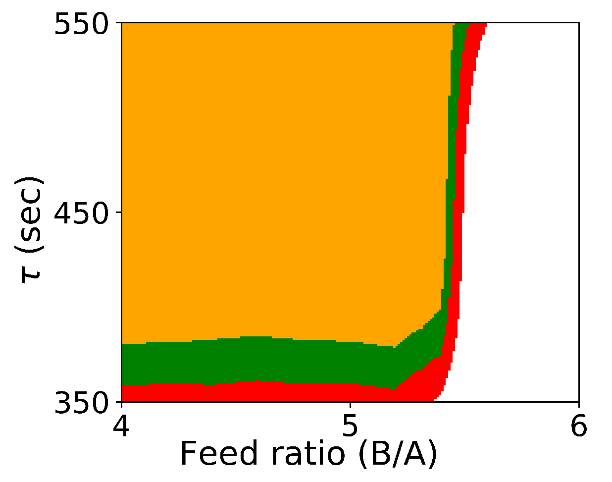
In this study, the initial concentrations $\left\{c_A^0,c_B^0,c_C^0,c_D^0,c_E^0\right\}$ are set to be $\left\{0.53,0.53R_{B|A},0,0,0\right\}$ mol/L. The probabilistic design space is computed over $R_{B|A}$ (the ratio of the concentration of B to A in the feed) and the residence time $\tau$. That is ${\theta }_p=\{R_{B|A},\tau \}$. The process parameter space is discretized with $R_{B|A}$ ranging from 4 to 6, and the residence time $\tau$ ranging from 350 to 550 s, with 11 and 21 points respectively.

The feasibility of process operation is determined by the CQAs represented with the following inequality constraints:

$$\begin{array}{c}\hfill \frac{c_D}{c_A^0-c_A}\ge 0.9\Rightarrow 0.9c_A^0-0.9c_A-c_D\le 0\end{array}$$

(48)

$$\begin{array}{c}\hfill \frac{c_D}{c_A+c_B+c_C}\ge 0.2\Rightarrow c_A+c_B+c_C-5.0c_D\le 0\end{array}$$

(49)

The first equation states that the yield of product D must be greater than 90%. The second equation states that the ratio of the concentration of D to the concentration of unreacted species must be greater than 0.2.

For Equations (28)–(36), the model equations h are represented with Equations (39)–(40) and (43)–(47), and the CQAs are represented with Equations (48) and (49).

All timing results for Case Study 1 are shown in

Table 1. Timing results for Case Study 1 (in seconds).

Approach	Ipopt (Local)	BARON (Global)
Algorithm 1	2745.3	–
Algorithm 2 with Equation (21),	14.2	35.4
Algorithm 2 with Equation (24),	13.0	37.8
Algorithm 3 with Equation (33),	0.767	1.26
Algorithm 3 with Equation (34),	0.865	3.63

. Generating the probabilistic design space takes over 45 min using the Monte-Carlo approach and requires significantly more computational effort because of the large number of required simulations. The approaches in Algorithms 2 and 3 are significantly faster taking a little over 35 s and approximately 3 s respectively (using the global solver BARON). The approach using Algorithm 3 is significantly faster, however, recall that it restricts the shape of the probabilistic design space in ${\theta }_p$ to a hyperrectangle as will be seen in the figures later. While results with the local solver Ipopt are faster again (by about a factor of 2), recall that the local solver cannot provide guarantees that the size of the probabilistic design space may be overestimated. For this simple test case, we do not see significant differences in computational timing when formulating Equations (16)–(23) and Equations (28)–(36) with either the hyperrectangle or the ellipsoid constraint.

Figure 1 shows the probabilistic design space generated by Algorithm 1.

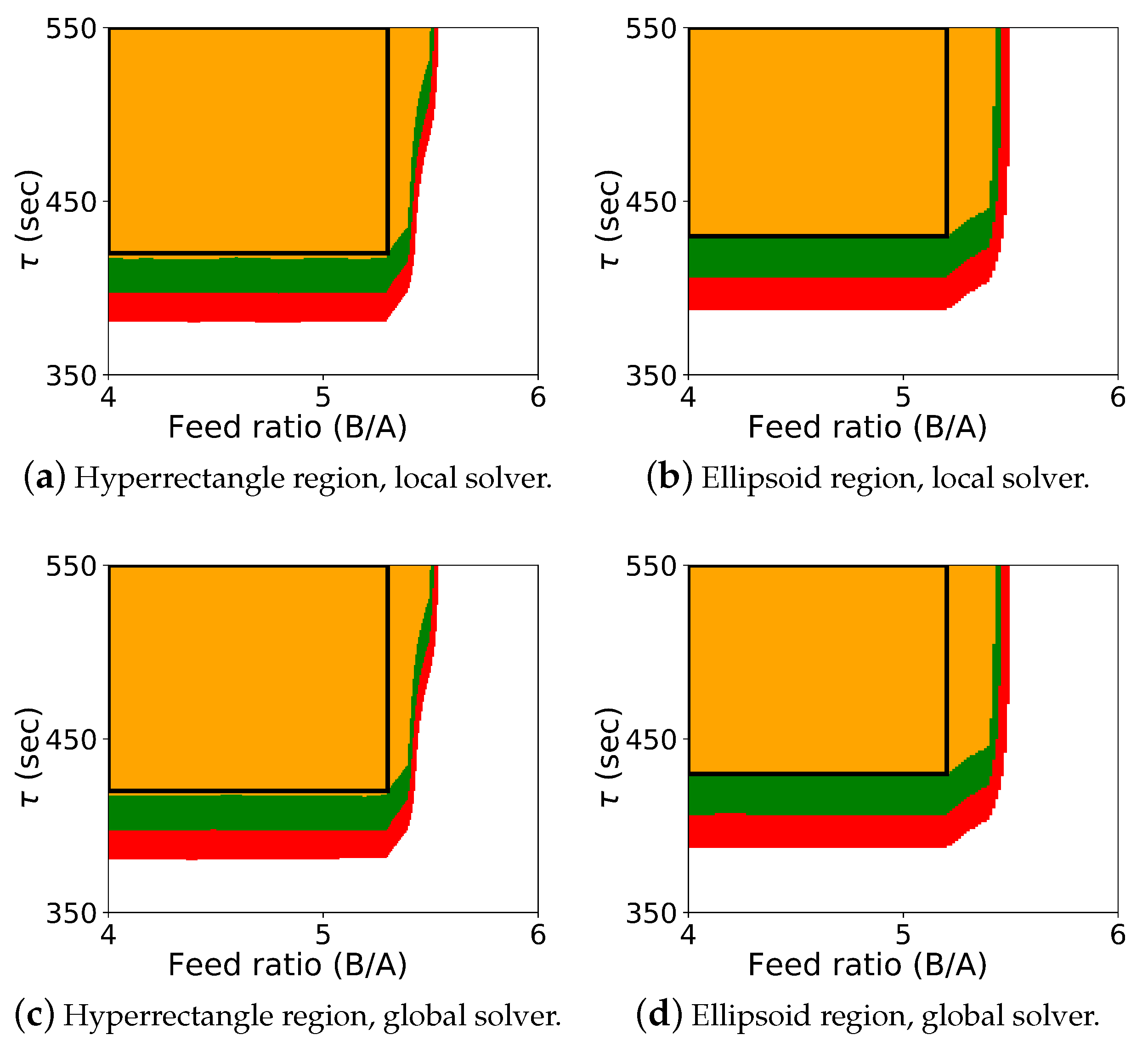
The results for the optimization-based flexibility methods are shown in Figure 2, and it includes results for both Algorithm 2 and Algorithm 3, shown for the hyperrectangle and the ellipsoid constraint with both the local solver Ipopt and the global solver BARON.

The colored map shows the probabilistic design space obtained using Algorithm 2, and the black rectangle shows the space identified by Algorithm 3 (generated with a single confidence level of $0.85$). In this case study, it was known that the upper left corner of the design space corresponded to the “safe” operating region with respect to the CQAs, and the values for ${\overline{\theta }}_p$, $\Delta {\theta }_p^{-}$, and $\Delta {\theta }_p^{+}$ could be effectively selected a priori. Also, since the shape of the probabilistic design space itself is also rectangular, the differences between the regions from Algorithm 2 and Algorithm 3 are not dramatic. These differences can be more pronounced with other case studies. For this case study, the probabilistic design space identified is similar using both the hyperrectangle and ellipsoid constraints, and the regions identified with the local and global solver are also very similar.

As expected, if we compare these results with the results from Algorithm 1 shown in Figure 1, we see that the design space from the flexibility-based methods is indeed more conservative. Consider results from Algorithm 2. While there are minor differences with respect to $R_{B|A}$, the lower value for $\tau$ corresponding to a confidence level of $0.85$ is approximately 375 for the Monte-Carlo approach and 425 for the flexibility-based approaches. 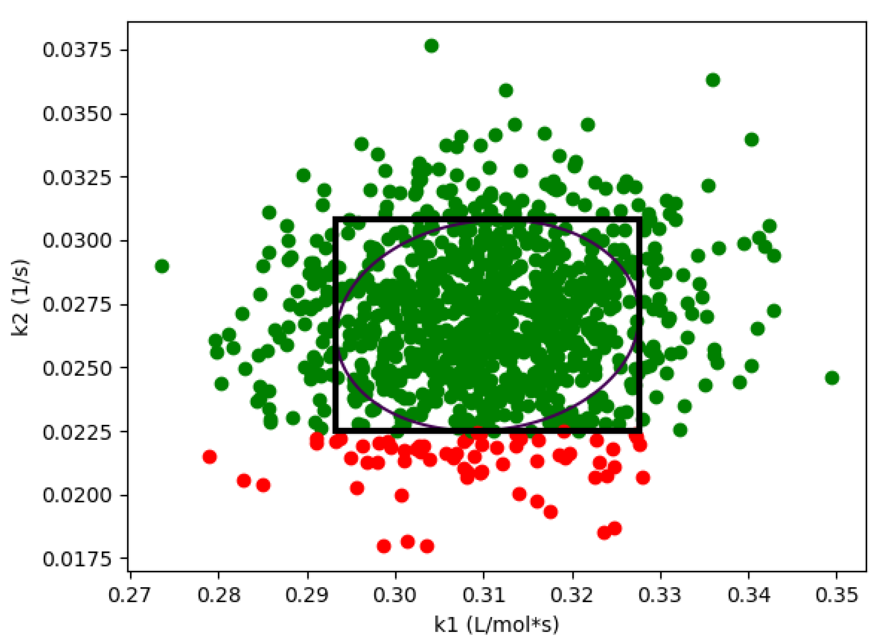This is because the shape of the flexibility region in ${\theta }_m$ is restricted. Consider a single point in the process parameter space. Figure 3 shows the results of 1000 simulations (from the Monte-Carlo approach), where the green points are feasible with respect to the CQAs, and red points are not. On this figure, we are also showing the hyperrectangle and ellipsoid generated with Algorithm 2. We can immediately see the impact of restricting the shape. Because of the constraints, the acceptable region for the CQAs in ${\theta }_m$ is not symmetric, and the Monte-Carlo approach is able to identify acceptable points that the flexibility-based approaches are not.

3.2. Case Study 2: Michael Addition Reaction

In this section, we consider an industrial case provided by the Eli Lilly and Company—the Michael addition reaction [27] with kinetics described in the following equations:

$$\begin{array}{c}\hfill AH+B\stackrel{k_1}{\to }{A}^{-}+B{H}^{+}\end{array}$$

(50)

$$\begin{array}{c}\hfill A^{-}+C\stackrel{k_2}{\to }A{C}^{-}\end{array}$$

(51)

$$\begin{array}{c}\hfill A{C}^{-}\stackrel{k_3}{\to }{A}^{-}+C\end{array}$$

(52)

$$\begin{array}{c}\hfill A{C}^{-}+AH\stackrel{k_4}{\to }{A}^{-}+P\end{array}$$

(53)

$$\begin{array}{c}\hfill A{C}^{-}+B{H}^{+}\stackrel{k_5}{\to }P+B\end{array}$$

(54)

where $AH$ (Michael donor) and C (Michael acceptor) are starting materials, B is a base, $B{H}^{+},A^{-}$ and $A{C}^{-}$ are reaction intermediates, and P is the product. Reaction rates $r_i$ are defined as follows:

$$\begin{array}{c}\hfill r_1=k_1{c}_{AH}{c}_B\end{array}$$

(55)

$$\begin{array}{c}\hfill r_2=k_2{c}_{A^{-}}{c}_C\end{array}$$

(56)

$$\begin{array}{c}\hfill r_3=k_3{c}_{A{C}^{-}}\end{array}$$

(57)

$$\begin{array}{c}\hfill r_4=k_4{c}_{A{C}^{-}}{c}_{AH}\end{array}$$

(58)

$$\begin{array}{c}\hfill r_5=k_5{c}_{A{C}^{-}}{c}_{B{H}^{+}}\end{array}$$

(59)

The rate constants $k_i$ are the uncertain model parameters (i.e., ${\theta }_m=\{k_1,k_2,k_3,k_4,k_5\}$), and these rate constants have estimated values,

$$\begin{array}{c}\hfill \widehat{k}=\left[\begin{array}{ccccc}49.7796& 8.9316& 1.3177& 0.3109& 3.8781\end{array}\right]\end{array}$$

and the multivariate normal variance-covariance matrix given by:

$$\left[\begin{array}{ccccc}1.005& -3.428\times {10}^{-4}& -1.006\times {10}^{-3}& -1.523\times {10}^{-3}& 2.718\times {10}^{-3}\\ -3.428\times {10}^{-4}& 0.412& 7.951\times {10}^{-4}& -3.937\times {10}^{-3}& 2.364\times {10}^{-3}\\ -1.006\times {10}^{-3}& -7.951\times {10}^{-4}& 3.224\times {10}^{-3}& 1.466\times {10}^{-3}& -2.400\times {10}^{-3}\\ -1.523\times {10}^{-3}& -3.937\times {10}^{-3}& 1.466\times {10}^{-3}& 2.746\times {10}^{-3}& -4.102\times {10}^{-3}\\ 2.718\times {10}^{-3}& 2.364\times {10}^{-3}& -2.400\times {10}^{-3}& -4.102\times {10}^{-3}& 7.148\times {10}^{-3}\end{array}\right]$$

(60)

Using a CSTR mass balance over the reactions, Equations (50)–(54), we may write the following equations:

$$\begin{array}{c}\hfill c_{AH}^0-c_{AH}+\tau \left(-r_1-r_4\right)=0\end{array}$$

(61)

$$\begin{array}{c}\hfill c_B^0-c_B+\tau \left(-r_1+r_5\right)=0\end{array}$$

(62)

$$\begin{array}{c}\hfill c_C^0-c_C+\tau \left(-r_2+r_3\right)=0\end{array}$$

(63)

$$\begin{array}{c}\hfill c_{A^{-}}^0-c_{A^{-}}+\tau \left(r_1-r_2+r_3+r_4\right)=0\end{array}$$

(64)

$$\begin{array}{c}\hfill c_{A{C}^{-}}^0-c_{A{C}^{-}}+\tau \left(r_2-r_3-r_4-r_5\right)=0\end{array}$$

(65)

$$\begin{array}{c}\hfill c_{B{H}^{+}}^0-c_{B{H}^{+}}+\tau \left(r_1-r_5\right)=0\end{array}$$

(66)

$$\begin{array}{c}\hfill c_P^0-c_P+\tau \left(r_4+r_5\right)=0\end{array}$$

(67)

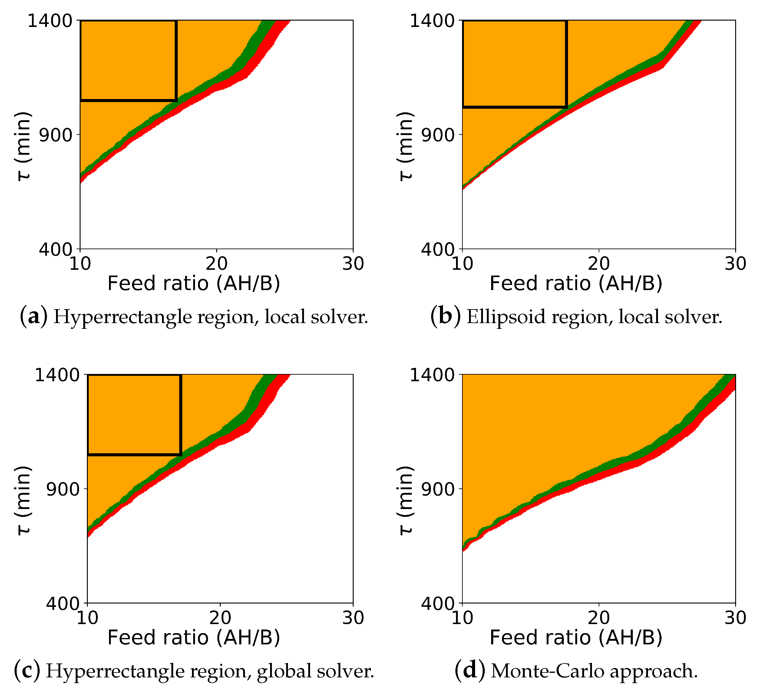
In this study, the initial concentrations $\left\{c_{AH}^0,c_B^0,c_C^0,c_{{BH}^{+}}^0,c_{A^{-}}^0,c_{{AC}^{-}}^0,c_P^0\right\}$ are set to be $\left\{0.3955,0.3955/R,0.25,0,0,0,0\right\}$ mol/L respectively, where R is the molar ratio between the feed concentration of AH and B. The process parameters include the molar ratio R and the residence time $\tau$ (i.e., ${\theta }_p=\{R,\tau \}$). These process parameters are discretized with R from 10 to 30, and $\tau$ from 400 to 1400 min, with 21 and 11 points respectively.

Feasible process operation is determined by the following two CQA constraints:

$$\begin{array}{c}\hfill \frac{c_C^0-c_C-c_{A{C}^{-}}}{c_C^0}\ge 0.9\Rightarrow c_C+c_{A{C}^{-}}-0.1\times c_C^0\le 0\end{array}$$

(68)

$$\begin{array}{c}\hfill c_{A{C}^{-}}\le 0.002\end{array}$$

(69)

The first constraint states that the conversion of feed C must be greater than 90%, and the second states that the concentration of $A{C}^{-}$ in the outlet must be less than 0.002 mol/L.

The model equations h are represented with Equations (55)–(59) and (61)–(67), and the CQAs are represented with Equations (68) and (69).

The timing results for this case study can be found in

Table 2. Timing results for Case Study 2 (in seconds).

Approach	Ipopt (Local)	BARON (Global)
Alg. 1	6116.2	–
Alg. 2 with Equation (21),	16.3	203
Alg. 2 with Equation (24),	18.0	–
Alg. 3 with Equation (33),	1.26	21.7
Alg. 3 with Equation (34),	1.65	245.3

.

Here we see similar results as with the first case study. The flexibility-based methods are significantly faster than the Monte-Carlo approach. As before, Algorithm 3 was about an order of magnitude faster than Algorithm 2. However, here we also see one of the challenges of the global optimization approaches. For the ellipsoidal constraint with Algorithm 2, BARON failed to converge for a small number of points, and therefore, timing results are not reported for this case. When using BARON with the ellipsoidal constraint in Algorithm 3, the gap did not close within the specified time limit on two iterations of the bisection method. However, when the maximum allowed time was reached for these two points, both the upper and lower bounds on the objective value were negative, signifying operational feasibility. The LDL transformation of the ellipsoid constraint was used in both formulations during global optimization.

The probabilistic design space generated from the Monte Carlo procedure and from the flexibility-based approaches is shown in Figure 4. As with case study 1, this figure includes results for both Algorithm 2 and Algorithm 3. Since BARON did not solve with the ellipsoidal constraint using Algorithm 2, this figure also includes the Monte-Carlo results in the subfigure (d).

As before, comparing the computed probabilistic design space, we see that Algorithm 2 is more conservative than the Monte-Carlo approach. Here, however, we see the more significant differences between the flexibility-based methods. The rectangular region produced by Algorithm 3 correctly lies inside the probabilistic design space produced by Algorithm 2. But, since the actual probabilistic design space is not rectangular, the rectangular region produced by Algorithm 3 significantly underestimates the size of the region. In some applications, the region that is to be reported may be defined with simple bounds on process parameters, and the rectangular region produced by Algorithm 3 will be sufficient. For other applications, this underestimation may be too dramatic, and extensions of this approach may need to be used to find a larger region (e.g., shifting the nominal point and producing multiple overlapping rectangles).

4. Discussion and Conclusions

A key component of the QbD initiative in the pharmaceutical industry is the identification of the probabilistic design space defined as the region in the space of the process parameters over which the critical quality attributes of the product are acceptable. Traditional Monte-Carlo approaches have been used to compute the probabilistic design space by discretizing the process parameters and performing simulations over hundreds (or more) of samples from the uncertain parameters.

Here, we proposed an optimization-based framework to define the probabilistic design space of a pharmaceutical process with model uncertainty using concepts from flexibility analysis [15,19]. Specifically, we proposed two methods. The first, Algorithm 2, is a direct application of the flexibility index formulation. This approach still discretizes the process parameters ${\theta }_p$, but replaces the Monte-Carlo simulations with a flexibility index formulation in the uncertain parameters ${\theta }_m$. The second approach solves for the probabilistic design space in ${\theta }_p$ directly, removing the need to discretize the process parameter space as well. Both these approaches showed significant improvement in computational performance over the Monte-Carlo approach, with Algorithm 3 being another order of magnitude faster than Algorithm 2. While the Monte-Carlo approach can be easily run in parallel, note that Algorithm 2 can also be run in parallel over the discretized points in ${\theta }_p$. Given the difference in solution time between the Monte-Carlo approach and Algorithm 3, it would take significant HPC resources to make the Monte-Carlo approach faster.

However, the size of the probabilistic design space produced by the flexibility-based approaches is more conservative since they restrict the shape of the confidence region in ${\theta }_m$ and, in the case of Algorithm 3, the shape of the probabilistic design space itself. It will depend on the specific application to determine if this trade-off is acceptable or not. Also, extensions of the flexibility test and flexibility index approaches could be used to reduce this effect.

Due to the problem definition, the formulations presented did not make use of online control action to increase the size of the probabilistic design space. The flexibility test and flexibility index formulations do provide rigorous treatment of controls [15,19,28], and future work will explore this aspect.

With case study 2 (Michael addition reaction), the global solver did not fully converge for either Algorithm 2 or Algorithm 3 when the ellipsoidal constraint in ${\theta }_m$ was used. While this constraint is convex, it was presented to the solver as a sum of bilinear terms, and it is possible that solver tuning or a straightforward outer-approximation would yield improved behavior.

As these problems become larger, performance of the global optimization step will become the primary bottleneck. One approach to improve performance is to instead solve a relaxation of Equations (16)–(23) or Equations (28)–(36). This will produce a design space that is more conservative, but the relaxations could be progressively refined (e.g., piecewise outer approximation) to manage the trade-off between the size of the design space and the computational effort of the approach.

This paper has shown that the concepts of flexibility analysis, and specifically the flexibility test and flexibility index formulations, can be used to compute probabilistic design spaces much more efficiently. Furthermore, there have been many advances in flexibility analysis that could be further applied to improve scalability and reduce conservativeness when estimating the design space.