Multiphase Open Phase Processes Differential Equations

Abstract

The thermodynamic approach for the description of multiphase open phase processes is developed based on van der Waals equation in the metrics of Gibbs and incomplete Gibbs potentials. Examples of thermodynamic modeling of the multiphase and multicomponent A³B⁵ systems (In-Ga-As-Sb and In-P-As-Sb) and Na⁺, K⁺, Mg²⁺, Ca²⁺//Cl⁻, SO₄²⁻-H₂O water–salt system are presented. Topological isomorphism of different type phase diagrams is demonstrated.

1. Introduction

It is common knowledge that conditions of phase equilibria shifts can be expressed in different mathematical forms, for example, as equality of the intense parameters of state first differentials (temperature, pressure and chemical potentials of components) in equilibrium (α, β) phases: dT^(α) = dT^(β); dP^(α) = dP^(β); dμ_i^(α) = dμ_i^(β) [1]. According to these conditions, van der Waals developed the differential equation for the description of phase equilibria shifts in the two-phase binary system [2]. Van der Waals equation allows obtaining the rules and laws characterizing the two-phase equilibrium in one-component and binary systems (Clausius–Clapeyron equation, Gibbs–Konovalov law, Gibbs–Roseboom rule, etc.). Storonkin expanded the van der Waals equation for multicomponent systems [3] and developed thermodynamic laws and rules for ternary, quaternary and more component systems (in particular, expanded Clausius–Clapeyron equation for the states characterized by equality of composition in equilibrium phases, van Rijn rule, hetero-azeotropes rule, Schreinemakers rule, etc.). Filippov et al. obtained the vector-matrix form of the van der Waals equation in the Gibbs potential metric [4,5]. Korjinskiy introduced the incomplete Gibbs potentials characteristic in the following set of variables: temperature, pressure, mole numbers and chemical potentials of the components [6]. Filippov et al. developed the vector-matrix form of van der Waals equation in the metric of incomplete Gibbs potential. In addition, they determined that the matrixes of the second concentration derivatives of Gibbs potential are nondegenerated and positively determined according to diffusional criterion of stability [4,5].

Charykova et al. [7] determined the absolute topological isomorphism of different types of phase diagrams (in particular, vapor–liquid equilibria at T = const and P = const, fusibility diagrams, solubility diagrams at T, P = const, etc.) in the complete and incomplete Gibbs potentials metrics. Phase processes can be divided into two classes:

(i) Close phase processes, when all masses of equilibrium phases coexist in equilibrium during the process. This case is trivial and does not require any additional equations, except classical mass balance equation: ${\displaystyle \sum _{i=1}^r[m^{(i)}d{\overrightarrow{x}}^{(i)}+}d{m}^{(i)}{\overrightarrow{x}}^{(i)}]=0$, where $m^{(i)},{\overrightarrow{x}}^{(i)}-$ mole number and composition vector of ith phase (in mole fraction concentration scale) and r is a total number of phases.

(ii) Open phase processes, when one or several equilibrium phases are continuously added or removed from the system. Gibbs developed the basic theory and equations for thermodynamic description of such processes [1]. Charykov et al. [8,9] obtained the vector form of differential equations for the description of open phase processes (for example, crystallization process) in the two phase and multiphase polyvariant systems.

The present article is devoted to the development of differential equations for thermodynamic description of different types of open phase processes. In addition, we demonstrate the application of these equations for calculation of open phase processes in multicomponent natural systems.

Van der Waals equations (equations of chemical equilibrium shift) and differential equations of open phase processes, obtained in this article, can be used for the following goals:

-

To test corresponding experimental data, concerning phase equilibrium diagrams and open phase processes diagrams; and

-

To predict phase equilibrium diagrams and open phase processes diagrams in multicomponent systems, using modeling parameters of non-ideality, determined later from available experimental data in binary and rarely in ternary subsystems.

In the article, the authors consequently consider

-

Generalized differential equation of phase equilibrium shifts (van der Waals Equation in Vector-Matrix Form) in the metrics of Gibbs and incomplete Gibbs potentials;

-

Differential equations of the open phase processes for two phase and multiphase equilibrium;

-

Differential equations of open phase processes in isothermal, isobaric and isothermo-isobaric conditions;

-

Non-extreme properties of the driving force parameters in the open phase processes; and

-

Some examples of thermodynamic semi-empirical modeling, based on the numerical integration of differential equations of open phase processes in multicomponent semiconductor A³-B⁵ and water–salt systems.

The manuscript is organized as follows: We first describe generalized differential equation of phase equilibrium shifts, van der Waals Equation and common differential equations of open phase processes in isothermal, isobaric and isothermo-isobaric conditions, both in vector-matrix form in the metrics of complete and incomplete Gibbs potentials. The second part of the article presents examples of the application of these differential equations to the description of open phase processes in multicomponent semiconductor (A³-B⁵) and water–salt systems.

2. Generalized Differential Equation of Phase Equilibrium Shifts (Van Der Waals Equation in Vector-Matrix Form)

2.1. Metric of Gibbs Potential

Let us consider the two-phase (α–β) equilibria in the n-component system. In metrics of Gibbs potential, the following parameters are independent variables of phases state: temperature (T), pressure (P) and mole numbers of components (or molar fractions,). The description of the two-phase (α–β) equilibrium shift can be given by the following system of differential van der Waals equations in the vector-matrix form [4,5]:

$$\begin{array}{ll}({\overrightarrow{x}}^{(\beta )}-{\overrightarrow{x}}^{(\alpha )}){\widehat{G}}^{(a)}d{\overrightarrow{x}}^{(a)}=& [S^{(a)}-S^{(\beta )}+({\overrightarrow{x}}^{(\beta )}-{\overrightarrow{x}}^{(\alpha )})\nabla S^{(a)}]dT\\ & -[V^{(a)}-V^{(\beta )}+({\overrightarrow{x}}^{(\beta )}-{\overrightarrow{x}}^{(\alpha )})\nabla V^{(a)}]dP\end{array}$$

(1)

$$\begin{array}{ll}({\overrightarrow{x}}^{(\alpha )}-{\overrightarrow{x}}^{(\beta )}){\widehat{G}}^{(\beta )}d{\overrightarrow{x}}^{(\beta )}=& [S^{(\beta )}-S^{(\alpha )}+({\overrightarrow{x}}^{(\alpha )}-{\overrightarrow{x}}^{(\beta )})\nabla S^{(\beta )}]dT\\ & -[V^{(\beta )}-V^{(\alpha )}+({\overrightarrow{x}}^{(\alpha )}-{\overrightarrow{x}}^{(\beta )})\nabla V^{(\beta )}]dP\end{array}$$

(2)

$${\widehat{G}}^{(a)}d{\overrightarrow{x}}^{(a)}-\nabla S^{(a)}dT+\nabla V^{(a)}dP={\widehat{G}}^{(\beta )}d{\overrightarrow{x}}^{(\beta )}-\nabla S^{(\beta )}dT+\nabla V^{(\beta )}dP$$

(3)

where $V^{(\tau )}$ and $S^{(\tau )}$ are the molar volumes and entropies of phases (τ = α or β); $\nabla V^{(\tau )}$ and $\nabla S^{(\tau )}$ are the gradients of these last properties with the concentration ${(\partial V^{(\tau )}/\partial x_i^{(\tau )})}_{T,P,x_k^{(\tau )}\ne X_{i,n}^{(\tau )}}$ and ${(\partial S^{(\tau )}/\partial x_i^{(\tau )})}_{T,P,X_k^{(\tau )}\ne X_{i,n}^{(\tau )}}$); ${\overrightarrow{x}}^{(\tau )}$ is a vector, characterizing the state of the figurative point of the τ phase in the concentration space; $d{\overrightarrow{x}}^{(\tau )}$ is a vector characterizing the displacement of ${\overrightarrow{x}}^{(\tau )}$ according to displacement of the two-phase equilibrium; and ${\widehat{G}}^{(\tau )}$ is an operator, corresponding to the matrix of the second derivatives $G_{ij}^{(\tau )}$:

$$G_{ij}^{(\tau )}={\left(\frac{\partial {}^2{G}^{(\tau )}}{\partial x_i^{(\tau )}\partial x_j^{(\tau )}}\right)}_{T,P,x_{k\ne j,n}}$$

(4)

where $G^{(\tau )}$ is the molar Gibbs energy potential of the τ phase. According to the phase stability criterion, the matrices of the ${\widehat{G}}^{(\tau )}$ operators and corresponding quadratic bilinear forms are nondegenerate and positively defined. Equations (1) and (2) expressed in the variables of (α) and (β) phases are equivalent. Equation (3) is a condition of phase equilibrium shift.

Parameters $S^{(\alpha \to \beta )}=[S^{(a)}-S^{(\beta )}+({\overrightarrow{x}}^{(\beta )}-{\overrightarrow{x}}^{(\alpha )})\nabla S^{(a)}]$ and $V^{(\alpha \to \beta )}=[V^{(a)}-V^{(\beta )}+({\overrightarrow{x}}^{(\beta )}-{\overrightarrow{x}}^{(\alpha )})\nabla V^{(a)}]$ have the physical sense of entropy and volume changes in the process of the isothermo-isobaric formation of one mole of β phase from infinitely large mass of α phase.

2.2. Metric of Incomplete Gibbs Potential (Korjinskiy Potential)

Filippov et al. developed van der Waals differential equations (Equations (6)–(8)) in the metric of incomplete Gibbs potential (Korjinskiy potential, see Equation (5)) defined as a function of the following natural parameters—temperature (T), pressure (P), mole numbers of the first k-components (n₁, n₂, …, n_k) and chemical potentials of the rest components (μ_k+1, μ_k+2,…,μ_n) [6,10]:

$$G_{[k]}=G-{\displaystyle \sum _{i=k+1}^n{n}_i{\mu }_i}={\displaystyle \sum _{i=1}^k{n}_i{\mu }_i}$$

(5)

$$\begin{array}{l}({\overrightarrow{Y}}^{(\alpha )}-{\overrightarrow{Y}}^{(\beta )}){\widehat{G}}_{[k]}^{(\beta )}d{\overrightarrow{Y}}^{(\beta )}=[{\tilde{S}}^{(\beta )}-{\tilde{S}}^{(\alpha )}+({\overrightarrow{Y}}^{(\alpha )}-{\overrightarrow{Y}}^{(\beta )})\nabla {\tilde{S}}^{(\beta )}]dT-[{\tilde{V}}^{(\beta )}-{\tilde{V}}^{(\alpha )}\\ +({\overrightarrow{Y}}^{(\alpha )}-{\overrightarrow{Y}}^{(\beta )})\nabla {\tilde{V}}^{(\beta )}]dP+{\displaystyle \sum _{q=k+1}^n\left[n_q^{(\beta )}-n_q^{(\alpha )}+({\overrightarrow{Y}}^{(\alpha )}-{\overrightarrow{Y}}^{(\beta )})\nabla n_q^{(\beta )}\right]}d{\mu }_q\end{array}$$

(6)

$$\begin{array}{l}({\overrightarrow{Y}}^{(\beta )}-{\overrightarrow{Y}}^{(\alpha )}){\widehat{G}}_{[k]}^{(\alpha )}d{\overrightarrow{Y}}^{(\alpha )}=[{\tilde{S}}^{(\alpha )}-{\tilde{S}}^{(\beta )}+({\overrightarrow{Y}}^{(\beta )}-{\overrightarrow{Y}}^{(\alpha )})\nabla {\tilde{S}}^{(\alpha )}]dT-[{\tilde{V}}^{(\alpha )}-{\tilde{V}}^{(\beta )}\\ +({\overrightarrow{Y}}^{(\beta )}-{\overrightarrow{Y}}^{(\alpha )})\nabla {\tilde{V}}^{(\alpha )}]dP+{\displaystyle \sum _{q=k+1}^n\left[n_q^{(\alpha )}-n_q^{(\beta )}+({\overrightarrow{Y}}^{(\beta )}-{\overrightarrow{Y}}^{(\alpha )})\nabla n_q^{(\alpha )}\right]}d{\mu }_q\end{array}$$

(7)

$$\begin{array}{l}{\widehat{G}}_{[k]}^{(\alpha )}d{\overrightarrow{Y}}^{(\alpha )}-\nabla {\tilde{S}}^{(\alpha )}dT+\nabla {\tilde{V}}^{(\alpha )}dP-{\displaystyle \sum _{q=k+1}^n\nabla n_q^{(\alpha )}d{\mu }_q}\\ ={\widehat{G}}_{[k]}^{(\beta )}d{\overrightarrow{Y}}^{(\beta )}-\nabla {\tilde{S}}^{(\beta )}dT+\nabla {\tilde{V}}^{(\beta )}dP-{\displaystyle \sum _{q=k+1}^n\nabla n_q^{(\beta )}d{\mu }_q}\end{array}$$

(8)

Evidently, the designations in Equations (1)–(3) are similar to those in Equations (6)–(8), but in the latest case the G_[k], S and V functions are referred to one mole of the first k components, and the ${\overrightarrow{Y}}^{(\tau )}$ vectors characterize the position of figurative point of the τ phase (α or β) in the reduced (k − 1)-dimensional concentration space:

$$y_i^{(\tau )}=n_i^{(\tau )}/{\displaystyle \sum _{j=1}^k{n}_j^{(\tau )}}\hspace{1em}\hspace{1em}\hspace{1em}\hspace{1em}\left({\displaystyle \sum _{i=1}^k{y}_i^{(\tau )}}=1\right)$$

(9)

Matrices $G_{[k]ij}^{(\tau )}$ are also nondegenerate, and the corresponding quadratic bilinear forms are positively determined according to Sylvester’s criterion [4,5,11].

$$G_{[k]ij}^{(\tau )}={\left(\frac{\partial {}^2{G}_{[k]}^{(\tau )}}{\partial y_i^{(\tau )}\partial y_j^{(\tau )}}\right)}_{T,P,y_{l\ne j,k}},$$

(10)

Parameters ${\tilde{S}}^{(\alpha \to \beta )}=[{\tilde{S}}^{(a)}-{\tilde{S}}^{(\beta )}+({\overrightarrow{Y}}^{(\beta )}-{\overrightarrow{Y}}^{(\alpha )})\nabla {\tilde{S}}^{(a)}]$, ${\tilde{V}}^{(\alpha \to \beta )}=[{\tilde{V}}^{(a)}-{\tilde{V}}^{(\beta )}+({\overrightarrow{Y}}^{(\beta )}-{\overrightarrow{Y}}^{(\alpha )})\nabla {\tilde{V}}^{(a)}]$ and $n_q^{(\alpha \to \beta )}=[n_q^{(\alpha )}-n_q^{(\beta )}+({\overrightarrow{Y}}^{(\beta )}-{\overrightarrow{Y}}^{(\alpha )})\nabla n_q^{(\alpha )}]$ are the changes of entropy, volume and number of moles (of the last k+1, k+2…n components), respectively, in the process of the isothermo-isobaric formation of one mole of β phase from infinitely big amount of the α phase taking into account only the masses of the first k components.

2.3. Multiphase Equilibria

Let us consider the equilibrium shift in r-phase (r $\ge$ 2). The bottom index (1) refers to the phase containing the maximal number of components. As a rule, the liquid phase consists of the maximal number of components because solid and vapor phases often have the constant composition. For example, in A^3-1 - A^3-2 -…-A^3-N—B^5-1 - B^5-2 -…- B^5-M (A^3-I = Al, Ga, In, etc.; B^5-I = P, As, Sb, Bi, etc.), the liquid phase (melt) consists of (N + M) components and the solid solutions (s) only (N + M − 1) components due to constraint equation: ${\displaystyle \sum _{I=1}^N{X}_{A^{3-I}}^{(s)}}={\displaystyle \sum _{I=1}^M{X}_{B^{5-I}}^{(s)}}=1/2$.

In this case, the system of van der Waals equations for the equilibria of the phases pairs (1-2; 1-3; 1-4…1-r) in the variables of (1) phase is the following:

(i) In the metric of Gibbs potential

$$\begin{array}{l}({\overrightarrow{x}}^{(2)}-{\overrightarrow{x}}^{(1)}){\widehat{G}}^{(1)}d{\overrightarrow{x}}^{(1)}=S^{(1\to 2)}dT-V^{(1\to 2)}dP\\ ({\overrightarrow{x}}^{(3)}-{\overrightarrow{x}}^{(1)}){\widehat{G}}^{(1)}d{\overrightarrow{x}}^{(1)}=S^{(1\to 3)}dT-V^{(1\to 3)}dP\\ ........................................................................\\ ({\overrightarrow{x}}^{(r)}-{\overrightarrow{x}}^{(1)}){\widehat{G}}^{(1)}d{\overrightarrow{x}}^{(1)}=S^{(1\to r)}dT-V^{(1\to r)}dP\end{array}$$

(11)

(ii) In the metric of incomplete Gibbs potential

$$\begin{array}{l}({\overrightarrow{Y}}^{(2)}-{\overrightarrow{Y}}^{(1)}){\widehat{G}}_{[k]}^{(1)}d{\overrightarrow{Y}}^{(1)}={\tilde{S}}^{(1\to 2)}dT-{\tilde{V}}^{(1\to 2)}dP+{\displaystyle \sum _{q=k+1}^n{n}_q^{(1\to 2)}}d{\mu }_q\\ ({\overrightarrow{Y}}^{(3)}-{\overrightarrow{Y}}^{(1)}){\widehat{G}}_{[k]}^{(1)}d\overrightarrow{Y}={\tilde{S}}^{(1\to 3)}dT-{\tilde{V}}^{(1\to 3)}dP+{\displaystyle \sum _{q=k+1}^n{n}_q^{(1\to 3)}}d{\mu }_q\\ .................................................................................................\\ ({\overrightarrow{Y}}^{(r)}-{\overrightarrow{Y}}^{(1)}){\widehat{G}}_{[k]}^{(1)}d\overrightarrow{Y}={\tilde{S}}^{(1\to r)}dT-{\tilde{V}}^{(1\to r)}dP+{\displaystyle \sum _{q=k+1}^n{n}_q^{(1\to r)}}d{\mu }_q\end{array}$$

(12)

Equations (11) and (12) are the systems of (1-2-3…r)-phase equilibria shifts in the metrics of different potentials.

3. Differential Equations of the Open Phase Processes

3.1. Two-Phase Processes

Let us formulate the differential equation of the two-phase (α–β) open phase process in vector form. The mass balance equation in the metric of Gibbs potential metric is the following:

$${\overrightarrow{x}}^{(\alpha )}=(1-d{m}^{(\beta )})({\overrightarrow{x}}^{(\alpha )}+d{\overrightarrow{x}}^{(\alpha )})+d{m}^{(\beta )}{\overrightarrow{x}}^{(\beta )}$$

(13)

where m^(β) is a mole number of β-phase formed from one mole of α-phase.

After neglecting the $d{m}^{(\beta )}d{\overrightarrow{x}}^{(\alpha )}$ second-order small term. one can get the equation:

$$d{\overrightarrow{x}}^{(\alpha )}=-({\overrightarrow{x}}^{(\beta )}-{\overrightarrow{x}}^{(\alpha )})d{m}^{(\beta )}$$

(14)

where $({\overrightarrow{x}}^{(\alpha )}-{\overrightarrow{x}}^{(\beta )})$ is a node vector, connecting the figurative points of coexisting equilibrium phases.

The mass balance equation in the metric of Korjinskiy potential is the following:

$$d{\overrightarrow{Y}}^{(\alpha )}=-({\overrightarrow{Y}}^{(\beta )}-{\overrightarrow{Y}}^{(\alpha )})d{\tilde{m}}^{(\beta )}$$

(15)

where $d{\tilde{m}}^{(\beta )}$ is a mole number of β-phase formed from one mole of α-phase (taking into account the first k components), and $({\overrightarrow{Y}}^{(\alpha )}-{\overrightarrow{Y}}^{(\beta )})$ is quasi-node vector connecting the figurative points of coexisting equilibrium phases in reduced (k − 1)-dimension concentration space.

3.2. Multiphase Processes

Let us formulate the vector form of differential equation of multiphase (1–2–…–r) open phase process for the description of r-phase equilibrium shifts (r $\ge$ 2). In this case, the mass balance equation is the following:

$${\overrightarrow{x}}^{(1)}=(1-{\displaystyle \sum _{i=2}^r}d{m}^{(i)})({\overrightarrow{x}}^{(1)}+d{\overrightarrow{x}}^{(1)})+{\displaystyle \sum _{i=2}^r}d{m}^{(i)}{\overrightarrow{x}}^{(i)}$$

(16)

where dm⁽²⁾, dm⁽³⁾…dm^(r) are the mole numbers of the 2,3…r phases formed from one mole of α-phase.

After neglecting the second-order small terms, one can get the equation:

$$d{\overrightarrow{x}}^{(i)}=-{\displaystyle \sum _{i=2}^r}({\overrightarrow{x}}^{(i)}-{\overrightarrow{x}}^{(1)})d{m}^{(i)}$$

(17)

where $({\overrightarrow{x}}^{(i)}-{\overrightarrow{x}}^{(1)})$ is a node vector and $({\overrightarrow{x}}^{(i)}-{\overrightarrow{x}}^{(j)})$, and $1\le i,j\le r;i\ne j$ is a nodes simplex (the set of all possible nodes). For example, in the case of two-phase system, it can be presented as a segment and in the case of three- and four-phase systems as triangle and tetrahedron, respectively.

Similarly, the mass balance equation in the metric of Korjinskiy potential is the following:

$$d{\overrightarrow{Y}}^{(i)}=-{\displaystyle \sum _{i=2}^r}({\overrightarrow{Y}}^{(i)}-{\overrightarrow{Y}}^{(1)})d{\tilde{m}}^{(i)}$$

(18)

where ${\tilde{m}}^{(i)}$ is a mass of ith phase (in mole numbers), considering only the first k components of the system.

4. Hybrid Differential Equations for Open Phase Processes

4.1. Two-Phase Systems

The combination of the open phase process equation (Equation (14)) and van der Waals equation in the Gibbs potential metric (Equation (1)) leads to Equation (19):

$$-({\overrightarrow{x}}^{(\beta )}-{\overrightarrow{x}}^{(\alpha )}){\widehat{G}}^{(\alpha )}({\overrightarrow{x}}^{(\beta )}-{\overrightarrow{x}}^{(\alpha )})d{m}^{(\beta )}=S^{(\alpha \to \beta )}dT-V^{(\alpha \to \beta )}dP$$

(19)

In addition, we can obtain the similar result based on differential equation of open phase process (Equation (14) and van der Waals equation in the metric of Korjinskiy potential (Equation (6)):

$$-({\overrightarrow{Y}}^{(\beta )}-{\overrightarrow{Y}}^{(\alpha )}){\widehat{G}}^{(a)}({\overrightarrow{Y}}^{(\beta )}-{\overrightarrow{Y}}^{(\alpha )})d{\tilde{m}}^{(\beta )}={\tilde{S}}^{(\alpha \to \beta )}dT-{\tilde{V}}^{(\alpha \to \beta )}dP+{\displaystyle \sum _{q=k+1}^n{n}_q^{(\alpha \to \beta )}}d{\mu }_q$$

(20)

4.2. Multiphase Systems

The substitution of differential equation for multiphase (1–2–…–r) open phase processes (Equation (17)) into the system of van der Waals Equation in the metric of Gibbs potential (Equation (11)) leads to the following system of equations:

$$\begin{array}{c}-({\overrightarrow{x}}^{(2)}-{\overrightarrow{x}}^{(1)}){\widehat{G}}^{(1)}{\displaystyle \sum _{i=2}^r}({\overrightarrow{x}}^{(i)}-{\overrightarrow{x}}^{(1)})d{m}^{(i)}=S^{(1\to 2)}dT-V^{(1\to 2)}dP\\ -({\overrightarrow{x}}^{(3)}-{\overrightarrow{x}}^{(1)}){\widehat{G}}^{(1)}{\displaystyle \sum _{i=2}^r}({\overrightarrow{x}}^{(i)}-{\overrightarrow{x}}^{(1)})d{m}^{(i)}=S^{(1\to 3)}dT-V^{(1\to 3)}dP\\ \dots \dots \dots \dots \dots \dots \dots \dots \dots \dots \dots \dots \dots \dots \dots \dots \dots \dots \dots \dots \dots \\ -({\overrightarrow{x}}^{(r)}-{\overrightarrow{x}}^{(1)}){\widehat{G}}^{(1)}{\displaystyle \sum _{i=2}^r}({\overrightarrow{x}}^{(r)}-{\overrightarrow{x}}^{(1)})d{m}^{(i)}=S^{(1\to r)}dT-V^{(1\to r)}dP\end{array}$$

(21)

Additionally, combining Equations (18) and (12) allows obtaining the following system of equations in the metric of Korjinskiy potential:

$$\begin{array}{c}-({\overrightarrow{Y}}^{(2)}-{\overrightarrow{Y}}^{(1)}){\widehat{G}}_{[k]}^{(1)}{\displaystyle \sum _{i=2}^r}({\overrightarrow{Y}}^{(i)}-{\overrightarrow{Y}}^{(1)})d{\tilde{m}}^{(i)}={\tilde{S}}^{(1\to 2)}dT-{\tilde{V}}^{(1\to 2)}dP+{\displaystyle \sum _{q=k+1}^n{n}_q^{(1\to 2)}}d{\mu }_q\\ -({\overrightarrow{Y}}^{(3)}-{\overrightarrow{Y}}^{(1)}){\widehat{G}}_{[k]}^{(1)}{\displaystyle \sum _{i=2}^r}({\overrightarrow{Y}}^{(i)}-{\overrightarrow{Y}}^{(1)})d{\tilde{m}}^{(i)}={\tilde{S}}^{(1\to 3)}dT-{\tilde{V}}^{(1\to 3)}dP+{\displaystyle \sum _{q=k+1}^n{n}_q^{(1\to 3)}}d{\mu }_q\\ \dots \dots \dots \dots \dots \dots \dots \dots \dots \dots \dots \dots \dots \dots \dots \dots \dots \dots \dots \dots \dots \dots \dots \dots \dots \dots \dots \dots \\ -({\overrightarrow{Y}}^{(r)}-{\overrightarrow{Y}}^{(1)}){\widehat{G}}_{[k]}^{(1)}{\displaystyle \sum _{i=2}^r}({\overrightarrow{Y}}^{(i)}-{\overrightarrow{Y}}^{(1)})d{\tilde{m}}^{(i)}={\tilde{S}}^{(1\to r)}dT-{\tilde{V}}^{(1\to r)}dP+{\displaystyle \sum _{q=k+1}^n{n}_q^{(1\to r)}}d{\mu }_q\end{array}$$

(22)

5. Open Phase Processes in Isothermal, Isobaric and Isothermo-Isobaric Conditions

5.1. Isobaric Conditions

The phase (β) formed in the open phase process should be continuously removed from phase equilibrium. Due to the isobaric conditions, the driving force of the process is temperature change or supplying-removal of heat. Let us consider the variants of realization of such isobaric open phase processes:

(i) Open evaporation with elimination of vapor. This process underlies the polythermal rectification column working. The typical case is two-phase systems, but we can also give a thermodynamic description for multiphase systems (equilibrium of several immiscible liquids with vapor phase or equilibrium of liquid phase with several immiscible vapors).

(ii) Open sublimation with elimination of vapor. As an example, this process can be realized in the polythermal sublimation column for the fullerenes mixtures (C₆₀ + C₇₀ + C₇₆ + C₇₈ + C₈₄ + …) separation. In the latest case, the two- and multiphase processes are possible.

(iii) Open crystallization of solid phases with constant compositions from the melts. Such phase processes are always open because only surfaces of formed crystals are in equilibrium with melts. Consequently, the deep crystal layers and crystal surface have different composition. As an example of realization of such processes, we can consider smelting of metals (the case of two-phase equilibrium) or the formation of geological rocks in the process of cooling of the Earth crust (liquid multiphase solids equilibrium).

(iv) Open crystallization of solid solutions from the melts. Similarly, such phase processes are open because only surfaces of formed solid solutions are in equilibrium with the melts. In real processes, we can neglect by diffusion in solid phases due to extremely low kinetic. The example of technical realization of such open phase processes is smelting of metal alloys or zone melting processes.

(v) Open crystallization of solid phases with constant composition or solid solutions from liquid solutions. Such processes can be realized during crystallization of evaporite minerals (NaCl, KCl, MgCl₂·6H₂O, Na₂SO₄·10H₂O, MgSO₄·7H₂O, Na₂SO₄·MgSO₄·4H₂O, etc.) from the modern evaporite basins under freezing in winter periods.

(vi) Open solid phase formation in the matrix of “old” solid phase. Due to a very slow solid phase diffusion, one can consider that only surface layers of growing solid phases are in equilibrium with the “old” solid phase.

Based on Equation (19) under isobaric conditions, we can obtain the following differential equations for the description of open phase process in two-phase systems:

$$\begin{array}{l}{(d{m}^{(\beta )}/dT)}_P=-S^{(\alpha \to \beta )}/[({\overrightarrow{x}}^{(\beta )}-{\overrightarrow{x}}^{(\alpha )}){\widehat{G}}^{(\alpha )}({\overrightarrow{x}}^{(\beta )}-{\overrightarrow{x}}^{(\alpha )})]\\ {(d{m}^{(\alpha )}/dT)}_P=-{(d{m}^{(\beta )}/dT)}_P\end{array}$$

(23)

In our conditions van der Waals differential Equations (1), (2) gives Equation (24):

$$\begin{array}{c}({\overrightarrow{x}}^{(\beta )}-{\overrightarrow{x}}^{(\alpha )}){\widehat{G}}^{(a)}d{\overrightarrow{x}}^{(a)}=S^{(a\to \beta )}dT\\ \hspace{1em}\hspace{1em}({\overrightarrow{x}}^{(\alpha )}-{\overrightarrow{x}}^{(\beta )}){\widehat{G}}^{(\beta )}d{\overrightarrow{x}}^{(\beta )}=S^{(\beta \to a)}dT\end{array}$$

(24)

The system in Equation (24) allows determining compositions and masses of both equilibrium phases (α and β).

Let us consider the system of differential equations in Equation (21) in isobaric conditions (dP = 0) for the description of the r-phase equilibria:

$$\begin{array}{c}{\displaystyle \sum _{i=2}^r({\overrightarrow{x}}^{(2)}-{\overrightarrow{x}}^{(1)}){\widehat{G}}^{(1)}}({\overrightarrow{x}}^{(i)}-{\overrightarrow{x}}^{(1)}){(d{m}^{(i)}/dT)}_P=-S^{(1\to 2)}\\ {\displaystyle \sum _{i=2}^r({\overrightarrow{x}}^{(3)}-{\overrightarrow{x}}^{(1)}){\widehat{G}}^{(1)}}({\overrightarrow{x}}^{(i)}-{\overrightarrow{x}}^{(1)}){(d{m}^{(i)}/dT)}_P=-S^{(1\to 3)}\\ \dots \dots \dots \dots \dots \dots \dots \dots \dots \dots \dots \dots \dots \dots \dots \dots \dots \dots \\ {\displaystyle \sum _{i=2}^r({\overrightarrow{x}}^{(r)}-{\overrightarrow{x}}^{(1)}){\widehat{G}}^{(1)}}({\overrightarrow{x}}^{(i)}-{\overrightarrow{x}}^{(1)}){(d{m}^{(i)}/dT)}_P=-S^{(1\to r)}\end{array}$$

(25)

The obtained system of equations can be solved by regarding ${(d{m}^{(i)}/dT)}_P$-derivative (2 ≤ i ≤ r) using the Cramer’s rule. Introducing the Gram determinant (see Equation (26))

$${\mathsf{\Delta }}_{Gr}^{(r-1)}=\left|\begin{array}{l}G{r}_{22}G{r}_{23}\dots G{r}_{2r}\\ G{r}_{32}G{r}_{33}\dots G{r}_{3r}\\ ...........................\\ G{r}_{r2}G{r}_{r3}\dots G{r}_{rr}\end{array}\right|;G{r}_{ij}=({\overrightarrow{x}}^{(i)}-{\overrightarrow{x}}^{(1)}){\widehat{G}}^{(1)}({\overrightarrow{x}}^{(j)}-{\overrightarrow{x}}^{(1)})$$

(26)

and S-substituted Gram determinant (Equation (27))

$${\mathsf{\Delta }}_{Gr-S-i}^{(r-1)}=\left|\begin{array}{l}G{r}_{22}G{r}_{23}\dots S^{(1\to 2)}\dots G{r}_{2r}\\ G{r}_{32}G{r}_{33}\dots S^{(1\to 3)}\dots G{r}_{3r}\\ ..........................................\\ G{r}_{r2}G{r}_{r3}\dots S^{(1\to r)}\dots G{r}_{rr}\end{array}\right|$$

(27)

allows obtaining the following expression for the ${(d{m}^{(i)}/dT)}_P$-derivative:

$${(d{m}^{(i)}/dT)}_P=-{\mathsf{\Delta }}_{Gr-S-i}^{(r-1)}/{\mathsf{\Delta }}_{Gr}^{(r-1)},{(d{m}^{(1)}/dT)}_P=-{\displaystyle \sum _{i=2}^r}{(d{m}^{(i)}/dT)}_P$$

(28)

The combination of the van der Waals differential equations (see Equations (24)) and Equation (28) allows determining the compositions and masses of all equilibrium phases (1,2,3…r). Masses of equilibrium phases in Equations (23) and (28) are natural parameters of state (or parameters of phase process). In addition, the mass balance differential equation for the description of open phase process is the following:

$${\displaystyle \sum _{i=2}^r{\mathsf{\Delta }}_{Gr-S-i}^{(r-1)}}/{\mathsf{\Delta }}_{Gr}^{(r-1)}={(d{m}^{(1)}/dT)}_P$$

(29)

5.2. Isothermal Conditions

In the case of isothermal conditions (T = const), the driving force of the process is a pressure change. Such open phase processes are comparatively rare, and we can provide only few examples:

(i) Open evaporation with vapor elimination. A technical device using such process is a standard polybaric rectification column, characterized by pressure decrease from bottom to top of the column. The typical case is a two-phase system, but we can also perform thermodynamic description of multiphase systems with immiscibility in liquid or vapor phases.

(ii) Open sublimation with vapor elimination.

(iii) Open phase processes with participation of only condensed phases are atypical because the moderate pressures do not considerably affect the condensed phases outside the critical state. In addition, the processes at high pressures (for example synthesis of detonation diamonds) cannot be realized as opened.

The differential equations of the open phase process in two-phase systems at constant temperature (dT = 0) are the following:

$$\begin{array}{l}{(d{m}^{(\beta )}/dP)}_T=V^{(\alpha \to \beta )}/[({\overrightarrow{x}}^{(\beta )}-{\overrightarrow{x}}^{(\alpha )}){\widehat{G}}^{(\alpha )}({\overrightarrow{x}}^{(\beta )}-{\overrightarrow{x}}^{(\alpha )})]\\ {(d{m}^{(\alpha )}/dP)}_T=-{(d{m}^{(\beta )}/dP)}_T\end{array}$$

(30)

Combining Equation (30) with the system of van der Waals equations (see Equation (31)) gives the following:

$$\begin{array}{c}({\overrightarrow{x}}^{(\beta )}-{\overrightarrow{x}}^{(\alpha )}){\widehat{G}}^{(a)}d{\overrightarrow{x}}^{(a)}=-V^{(a\to \beta )}dP\\ ({\overrightarrow{x}}^{(\alpha )}-{\overrightarrow{x}}^{(\beta )}){\widehat{G}}^{(\beta )}d{\overrightarrow{x}}^{(\beta )}=-V^{(\beta \to a)}dP\end{array}$$

(31)

Equation (31) can be used for determination of compositions and masses of both equilibrium phases (α and β).

Let us consider the system of Equation (21) at dT = 0 for the description of r-phase system:

$$\begin{array}{c}{\displaystyle \sum _{i=2}^r({\overrightarrow{x}}^{(2)}-{\overrightarrow{x}}^{(1)}){\widehat{G}}^{(1)}}({\overrightarrow{x}}^{(i)}-{\overrightarrow{x}}^{(1)}){(d{m}^{(i)}/dP)}_T=V^{(1\to 2)}\\ {\displaystyle \sum _{i=2}^r({\overrightarrow{x}}^{(3)}-{\overrightarrow{x}}^{(1)}){\widehat{G}}^{(1)}}({\overrightarrow{x}}^{(i)}-{\overrightarrow{x}}^{(1)}){(d{m}^{(i)}/dP)}_T=V^{(1\to 3)}\\ \dots \dots \dots \dots \dots \dots \dots \dots \dots \dots \dots \dots \dots \dots \dots \dots \dots \dots \\ {\displaystyle \sum _{i=2}^r({\overrightarrow{x}}^{(r)}-{\overrightarrow{x}}^{(1)}){\widehat{G}}^{(1)}}({\overrightarrow{x}}^{(i)}-{\overrightarrow{x}}^{(1)}){(d{m}^{(i)}/dP)}_T=V^{(1\to r)}\end{array}$$

(32)

Introduction of V-substituted Gram determinant (see Equation (33))

$${\mathsf{\Delta }}_{Gr-V-i}^{(r-1)}=\left|\begin{array}{l}G{r}_{22}G{r}_{23}\dots V^{(1\to 2)}\dots G{r}_{2r}\\ G{r}_{32}G{r}_{33}\dots V^{(1\to 3)}\dots G{r}_{3r}\\ .........................................\\ G{r}_{r2}G{r}_{r3}\dots V^{(1\to r)}\dots G{r}_{rr}\end{array}\right|$$

(33)

and considering Equation (26) allows obtaining the following equation for ${(d{m}^{(i)}/dP)}_T$ (2 ≤ i ≤ r) derivatives:

$${(d{m}^{(i)}/dP)}_T={\mathsf{\Delta }}_{Gr-V-i}^{(r-1)}/{\mathsf{\Delta }}_{Gr}^{(r-1)},{(d{m}^{(1)}/dP)}_T=-{\displaystyle \sum _{i=2}^r}{(d{m}^{(i)}/dP)}_T$$

(34)

The system in Equations (31) and (34) allows determining the compositions and masses of all equilibrium phases (1,2,…,r). Masses of equilibrium phases in Equations (31) and (34) are the natural parameters of state (parameters of phase process). In addition, the mass balance equation for the description of the open phase process is the following:

$${\displaystyle \sum _{i=2}^r{\mathsf{\Delta }}_{Gr-V-i}^{(r-1)}}/{\mathsf{\Delta }}_{Gr}^{(r-1)}=-{(d{m}^{(1)}/dP)}_T$$

(35)

5.3. Isothermo-Isobaric Conditions

In the case of the isothermo-isobaric conditions, the driving force of the process is change of chemical potential of the component. Such isothermo-isobaric open phase processes can be realized in the following cases:

(i) Open crystallization of both solid phases with constant composition or solid solutions from liquid phase in the process of evaporation of a single volatile component—solvent (for example, water). As an example of the technical realization of such processes, we can consider the crystallization of evaporite minerals from the natural brines during evaporation of water.

(ii) Precipitate formation (crystallization) in the process of salting out of the solid phase from solution by the second solvent characterized by very low solubility of the salts. Such processes can be realized during purification of the substances by (re)crystallization.

Let us consider the incomplete Gibbs potential (see Equation (5)) defined as a function of T, P, mole numbers of components (n₁, n₂,…, n_k−1) and chemical potentials of the nth component (μ_w):

$$G_{[w]}=G-n_n{\mu }_n={\displaystyle \sum _{i=1}^{n-1}{n}_i{\mu }_i}$$

(36)

the subindex “w” denotes the solvent molecule (for example, water).

Differential equations of the open phase process in the isothermo-isobaric conditions are the following in the case of two-phase systems:

$$\begin{array}{l}-({\overrightarrow{Y}}^{(\beta )}-{\overrightarrow{Y}}^{(\alpha )}){\widehat{G}}_{[\mathrm{w}]}^{(a)}({\overrightarrow{Y}}^{(\beta )}-{\overrightarrow{Y}}^{(\alpha )}){(d{\tilde{m}}^{(\beta )}/d{\mu }_w)}_{T,P}=n_w^{(\alpha \to \beta )}\\ {(d{\tilde{m}}^{(\alpha )}/d{\mu }_w)}_{T,P}=-{(d{\tilde{m}}^{(\beta )}/d{\mu }_w)}_{T,P}\end{array}$$

(37)

Combining Equation (37) with van der Waals equations (see Equations (6) and (7)) at dT = dP = 0 leads to Equation (38):

$$\begin{array}{c}({\overrightarrow{Y}}^{(\beta )}-{\overrightarrow{Y}}^{(\alpha )}){\widehat{G}}_{[w]}^{(\alpha )}d{\overrightarrow{Y}}^{(\alpha )}=n_w^{(\alpha \to \beta )}d{\mu }_w\\ ({\overrightarrow{Y}}^{(\alpha )}-{\overrightarrow{Y}}^{(\beta )}){\widehat{G}}_{[w]}^{(\beta )}d{\overrightarrow{Y}}^{(\beta )}=n_w^{(\beta \to \alpha )}d{\mu }_w\end{array}$$

(38)

Equation (38) allows determining the compositions and masses of both equilibrium phases (α and β).

Let us consider the system of differential equations (see Equation (22)) for r-phase system at dT = dP = 0:

$$\begin{array}{c}-{\displaystyle \sum _{i=2}^r({\overrightarrow{Y}}^{(2)}-{\overrightarrow{Y}}^{(1)}){\widehat{G}}_{[w]}^{(1)}}({\overrightarrow{Y}}^{(i)}-{\overrightarrow{Y}}^{(1)}){(d{\tilde{m}}^{(i)}/d{\mu }_w)}_{T,P}=n_w^{(1\to 2)}\\ -{\displaystyle \sum _{i=2}^r({\overrightarrow{Y}}^{(3)}-{\overrightarrow{Y}}^{(1)}){\widehat{G}}_{[w]}^{(1)}}({\overrightarrow{Y}}^{(i)}-{\overrightarrow{Y}}^{(1)}){(d{\tilde{m}}^{(i)}/d{\mu }_w)}_{T,P}=n_w^{(1\to 3)}\\ \dots \dots \dots \dots \dots \dots \dots \dots \dots \dots \dots \dots \dots \dots \dots \dots \dots \dots \dots \\ -{\displaystyle \sum _{i=2}^r({\overrightarrow{Y}}^{(r)}-{\overrightarrow{Y}}^{(1)}){\widehat{G}}_{[w]}^{(1)}}({\overrightarrow{Y}}^{(i)}-{\overrightarrow{Y}}^{(1)}){(d{\tilde{m}}^{(i)}/d{\mu }_w)}_{T,P}=n_w^{(1\to r)}\end{array}$$

(39)

In this case, the Gram determinant and μ_w-substituted Gram determinant can be expressed by Equations (40) and (41), respectively:

$${\tilde{\mathsf{\Delta }}}_{Gr}^{(r-1)}=\left|\begin{array}{l}G{\tilde{r}}_{22}G{\tilde{r}}_{23}\dots G{\tilde{r}}_{2r}\\ G{\tilde{r}}_{32}G{\tilde{r}}_{33}\dots G{\tilde{r}}_{3r}\\ ............................\\ G{\tilde{r}}_{r2}G{\tilde{r}}_{r3}\dots G{\tilde{r}}_{rr}\end{array}\right|;G{\tilde{r}}_{ij}=({\overrightarrow{Y}}^{(i)}-{\overrightarrow{Y}}^{(1)}){\widehat{G}}_{[w]}^{(1)}({\overrightarrow{Y}}^{(j)}-{\overrightarrow{Y}}^{(1)})$$

(40)

$${\tilde{\mathsf{\Delta }}}_{Gr-{\mu }_w-i}^{(r-1)}=\left|\begin{array}{l}G{\tilde{r}}_{22}G{\tilde{r}}_{23}\dots {\tilde{n}}_w^{(1\to 2)}\dots G{\tilde{r}}_{2r}\\ G{\tilde{r}}_{32}G{\tilde{r}}_{33}\dots {\tilde{n}}_w^{(1\to 3)}\dots G{\tilde{r}}_{3r}\\ ..........................................\\ G{\tilde{r}}_{r2}G{\tilde{r}}_{r3}\dots {\tilde{n}}_w^{(1\to r)}\dots G{\tilde{r}}_{rr}\end{array}\right|$$

(41)

The solution of differential Equation (39) by regarding ${(d{\tilde{m}}^{(i)}/d{\mu }_w)}_{T,P}$-derivative (2 ≤ i ≤ r) can be expressed as follows:

$${(d{\tilde{m}}^{(i)}/d{\mu }_w)}_{T,P}=-{\tilde{\mathsf{\Delta }}}_{Gr-{\mu }_w-i}^{(r-1)}/{\tilde{\mathsf{\Delta }}}_{Gr}^{(r-1)},{(d{\tilde{m}}^{(1)}/d{\mu }_w)}_{T,P}=-{\displaystyle \sum _{i=2}^r}{(d{\tilde{m}}^{(i)}/d{\mu }_w)}_{T,P}$$

(42)

Equations (38) and (42) allow determining the compositions and masses of all equilibrium phases (1,2,…,r). In addition, masses of equilibrium phases in Equations (37) and (42) are natural parameters of state (or parameters of the phase process). In addition, the mass balance equation of the open phase process can be expressed by Equation (43):

$${\displaystyle \sum _{i=2}^r{\tilde{\mathsf{\Delta }}}_{Gr-{\mu }_w-i}^{(r-1)}}/{\tilde{\mathsf{\Delta }}}_{Gr}^{(r-1)}={(d{\tilde{m}}^{(1)}/d{\mu }_w)}_{P,T}$$

(43)

5.4. Properties of the Driving Force Parameters in the Open Phase Processes

Based on the obtained theoretical results, we can conclude the following: (i) The driving forces (T, P and μ_w) cannot take the extremal values ($dT\ne 0,dP\ne 0,d{\mu }_w\ne 0$); in other words, Gram determinants should be non-zero defined (${\mathsf{\Delta }}_{Gr}^{(r-1)}\ne 0$,). (ii) Node vectors $({\overrightarrow{x}}^{(i)}-{\overrightarrow{x}}^{(1)})$ in the full concentration range or in the reduced concentration range $({\overrightarrow{Y}}^{(i)}-{\overrightarrow{Y}}^{(1)})$ should be linearly independent. Thus, the vectors of phase compositions in the full concentration range $({\overrightarrow{x}}^{(i)})$ or in the reduced concentration range $({\overrightarrow{Y}}^{(i)})$ should be linearly independent. (iii) It is necessary to state that, in the case of two-phase systems, we exclude from our consideration (independently of the component number): azeotropic points, points (curves, surfaces, hypersurfaces, etc.) characterized by extremum of the solid solutions melting temperature, congruent melting points of compounds with constant composition (with maximum of temperature), polymorph transformation points in solid phases, points of the solvent chemical potential extremum (always minimum of μ_w), points of congruent dissolution of compounds with constant composition (always maximum of μ_w), and solubility points of two different crystal solvates referred to the same compound. The above-mentioned cases can be described by the following equations:

$${(d{m}^{(i)}/dT)}_P=\infty ,\mathrm{or}{(d{m}^{(i)}/dP)}_T=\infty ,\mathrm{or}{(d{\tilde{m}}^{(i)}/d{\mu }_w)}_{T,P}=\infty$$

(44)

(iv) In the case of open phase processes in r-phase systems, we exclude from our consideration the following cases (independently of number of components): points, curves, surfaces, hyper-surfaces, and characterized by linear dependence of the phases composition (extremum T_P or P_T). Such peculiarities in phase diagrams take place in the following cases: fusibility diagrams of ternary systems (van Rijn points); three-phase equilibrium (liquid–liquid–vapor) curves in ternary systems, when figurative points of both liquids and vapor phases belong to the straight line; lines corresponding to equilibrium of the two different polymorph modifications of component (or compound) and melt in ternary systems; and geometrical images, where the reduced compositions of the phases (without taking into account the solvent) are linearly dependent (have extremum of (μ_w)_P,T). Such properties can be observed in the following cases: van Rijn points in solubility diagrams of quaternary systems; three-phase equilibrium (solid–solid–liquid) curves, when figurative points of both solid phases and liquid belong to the straight line; lines corresponding to equilibrium of two different solid crystal solvates (of component or compound) and liquid in the case of quaternary systems; the case when one of the equilibrium phases containing the maximal number of components reduces its number up to the value corresponding to the equilibrium phase with decreased number of components (the latest condition leads to extremum of T_P or P_T); and the case when one of the equilibrium phases containing the maximal number of components reduces its number up to the value corresponding to the equilibrium phase with decreased number of components (in the concentration space without solvent molecules). The latest conditions leads to (μ_w)_P,T extremum.

6. Examples of Thermodynamic Modeling

In our opinion, the developed differential equations are very convenient for calculation of open phase processes in real natural or technological systems. To this end, it is enough to determine the dependencies of Gibbs potentials on the parameters of state for all coexisting phases: $G(T,P,\overrightarrow{x}),G_{[w]}(T,P,\overrightarrow{Y},n_w)$. Since the standard functions of the components and compounds are well-known and tabulated, the main complicity is determining the excess thermodynamic functions of the solution in different aggregative states. For determination of excess thermodynamic functions, the following semi-empirical models can be used:

-

EFLCP model (Excess Functions = Linear Combinations of standard Chemical Potentials) [12,13] for the description of the excess functions in systems containing melts of A³-B⁵ semiconductors;

-

LDM (Lennard–Jones Model) or QRSM model (Quasi Regular Solution Model) [14,15] for the description of excess thermodynamic functions in systems, containing solid solutions of isovalent substitution (for example, in systems containing A³-B⁵ semiconductors) [12]; and

-

classical Pitzer’s model [16,17] for the description of excess functions in water–salt systems.

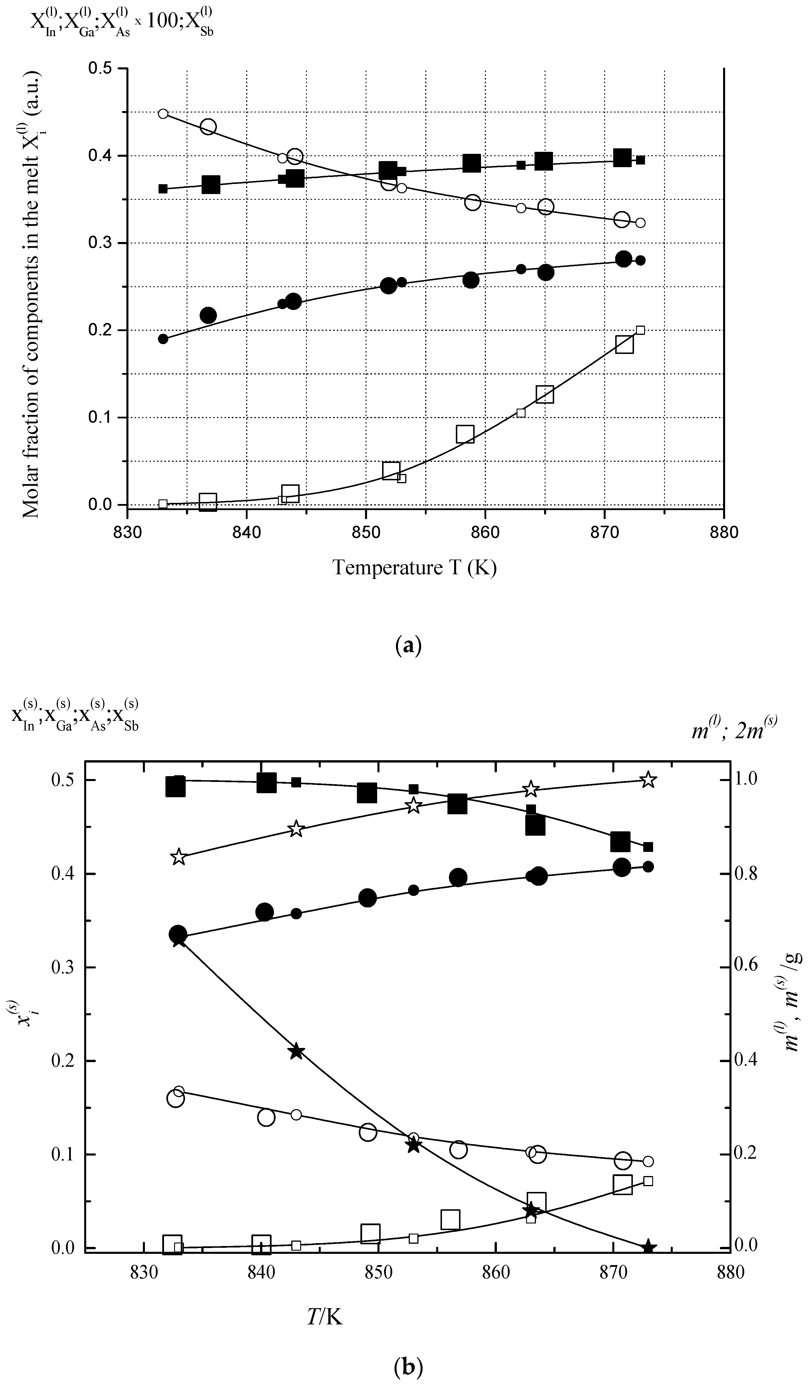
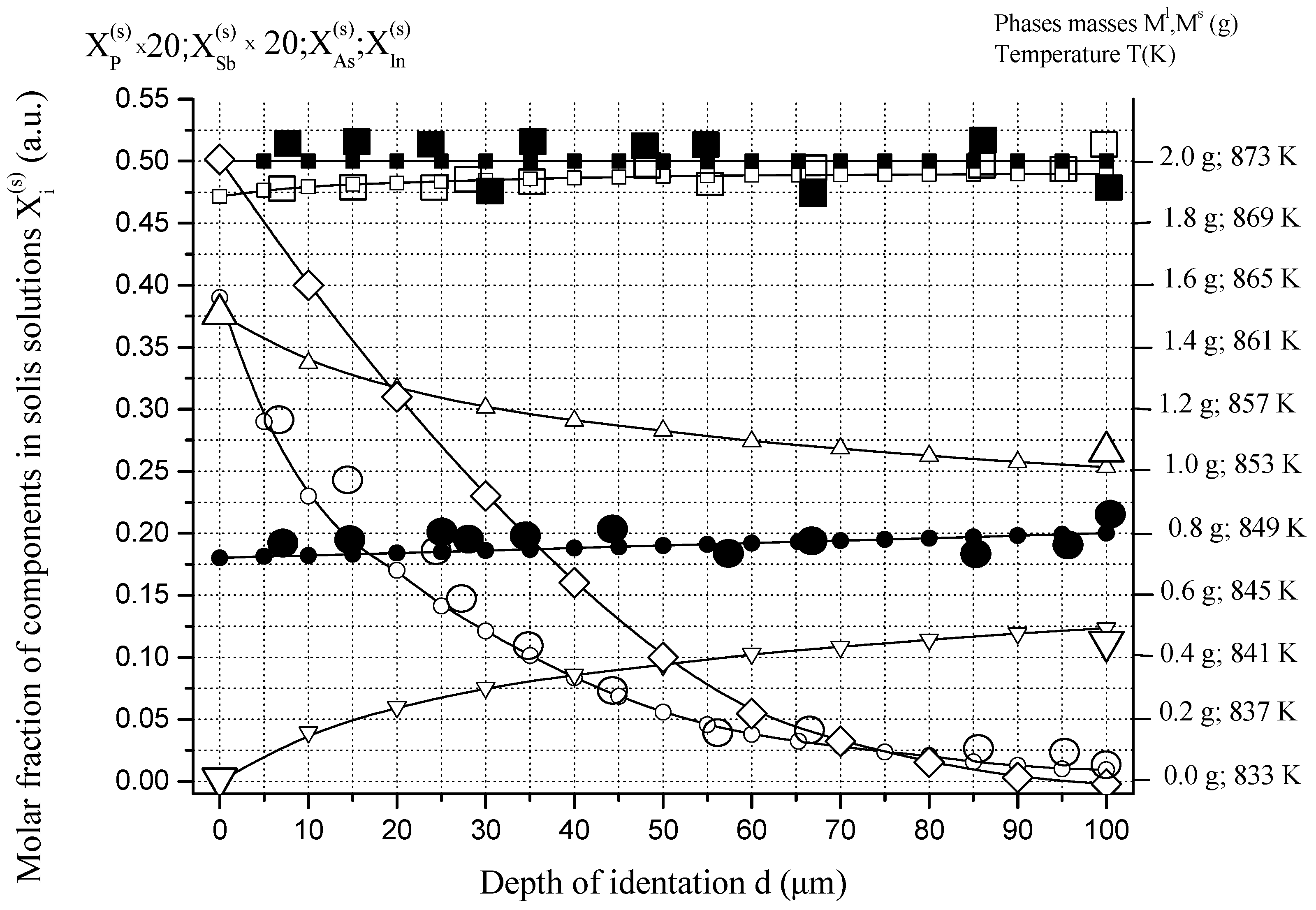
6.1. Two-Phase Open Crystallization in the In-Ga-As-Sb and In-P-As-Sb Systems at Temperature Decrease

Figure 1 presents open crystallization curves for the In-Ga-As-Sb system in the temperature range from 873 to 833 K obtained by LPE (Liquid Phase Epitaxy) from the quaternary melts by crystallization on the GaSb monocrystal substrate (1, 0, 0) [18]. The compositions of solid solutions were determined using the indentation plate by X-ray microanalysis in the form of x_i^(s)(d) dependencies (d is a plate thickness or depth of indentation). Obtained x_i^(s)(d) data were recalculated into the x_i^(s)(T) dependencies using experimental data on temperature dependence of the sample mass m^(s)(T) (in mole numbers) and Vegard’s low for the lattice parameter of solid solution (a):

$$a=4{\displaystyle \sum _{i=A^3=1}^2{\displaystyle \sum _{j=B^5=1}^2{x}_i^{(s)}{x}_j^{(s)}{a}_{ij}}}$$

(45)

where a_ij is a lattice period of the A_i³B_j⁵ compound (InAs, InSb, GaAs, GaSb). The molar volumes of solid solution and function d can be calculated as:

$$V^{(s)}=N_a{a}^3,d=1/S{\displaystyle \underset{T_1}{\overset{T_2}{\int }}{V}^{(s)}(T)/(d{m}^{(s)}/dT}{)}_{P}dT=1/S{\displaystyle \sum _{i(T_1)}^{i(T_2)}{V}_i{}^{(s)}(T)/d{m}_i{}^{(s)}/dT}$$

(46)

where S is a substrate area, i is a number of fragment of the solid solution growth, and i(T₁) and i(T₂) are the first and the last crystallization fragments. In addition, the data on melt composition can be calculated based on experimental data on composition and mass of solid solution using the mass balance equation for all melt components. The same procedure can be used for calculation of the crystallization curves in In-P-As-Sb system in the temperature range from 923 to 883 K (Figure 2) [18].

As standard functions of the components and compounds A³B⁵ in melts and solid phase (standard heats of formation, entropies and isobar heat capacities) are well-known, the parameters of non-ideality or excess thermodynamic functions (EFLCP and MLD (Lennard-Jones Model) show the strongest influence on the accuracy of modeling.

Here and when comparing the calculated and experimental data, deviations between them amounted to up to five relative percent.

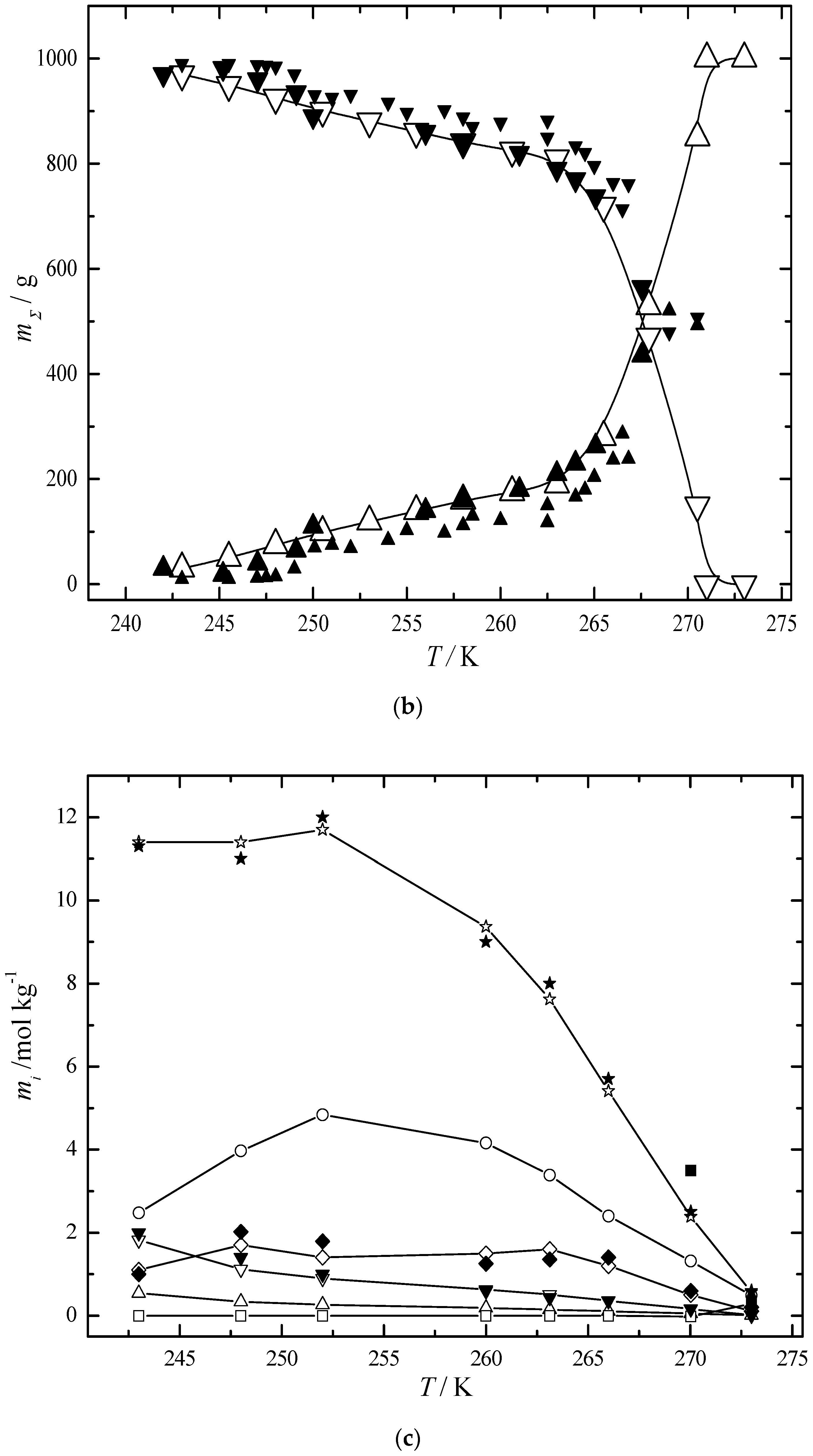
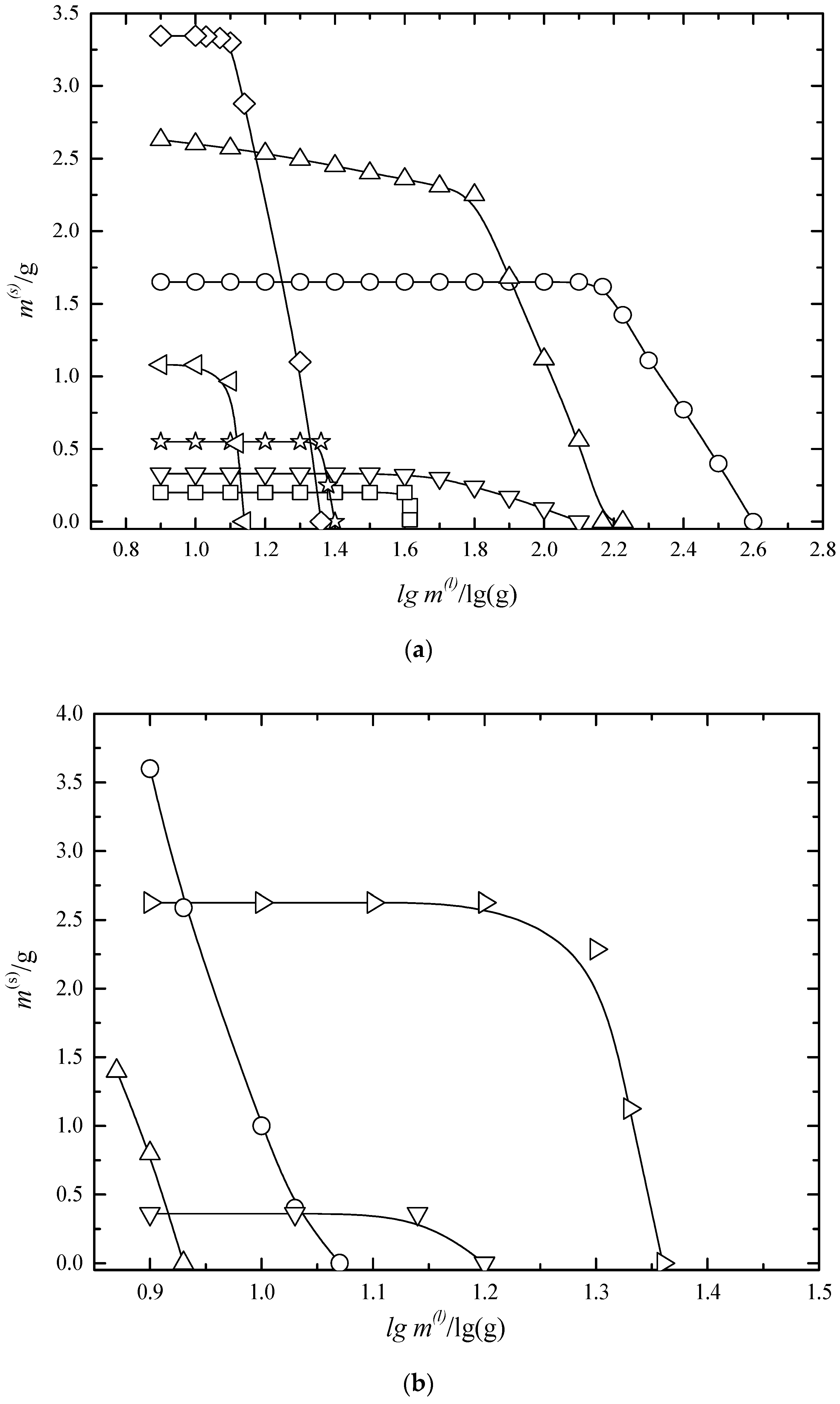
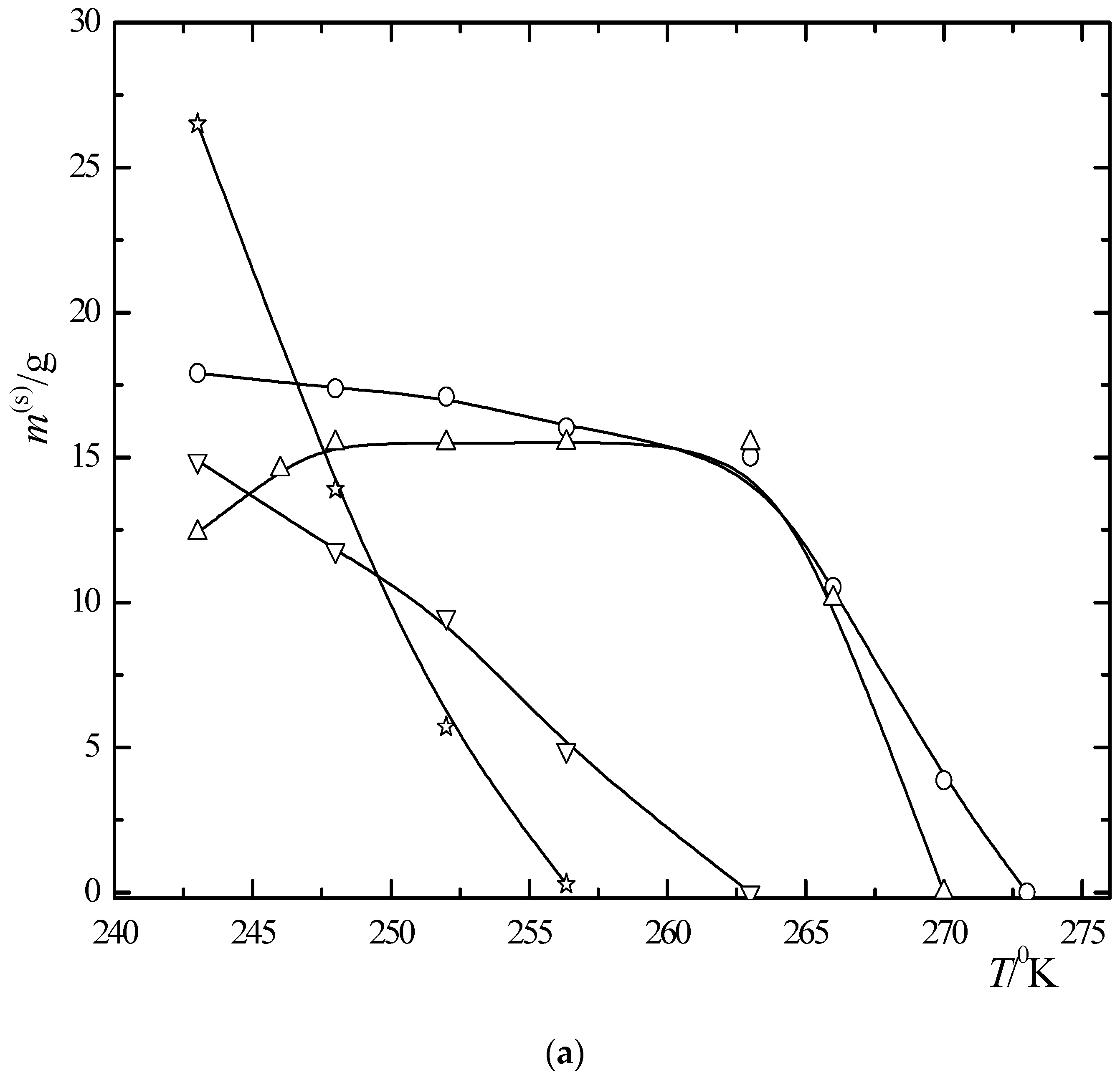
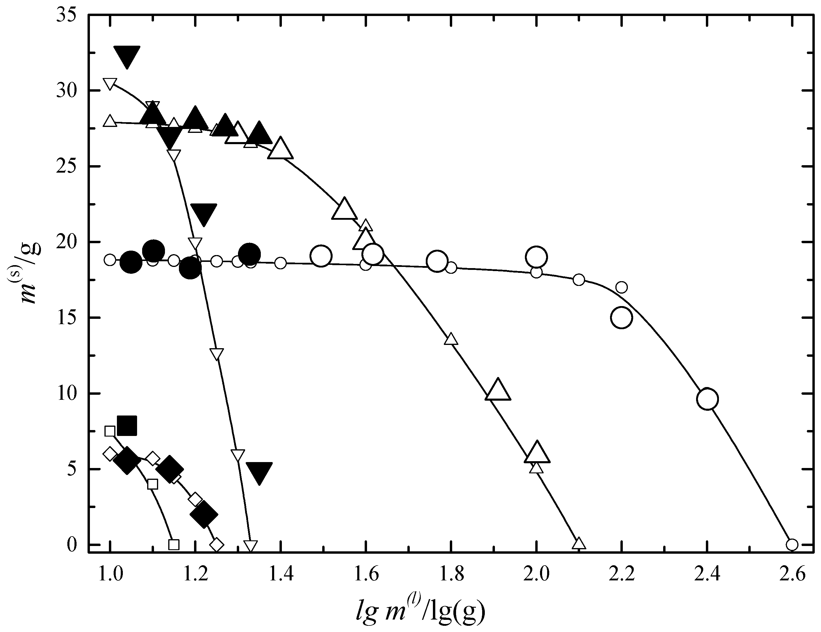
6.2. Multiphase Open Crystallization in the Na⁺, K⁺, Mg²⁺, Ca²⁺//Cl⁻, SO₄²⁻-H₂O System at Water Chemical Potential Decrease (Water Evaporation)

Figure 3 presents the open crystallization curves in Na⁺, K⁺, Mg²⁺, Ca²⁺//Cl⁻, SO₄²⁻-H₂O system at 298 K [7]. Chemical potential of water (μ_w)_P,T decreases in the range of water activity changing from 0.9416 to 0.3195. In addition, the chemical potential monotonically decreases in the process of open crystallization:

$${\mu }_w={\mu }_w{}^{(0)}+RT\ln a_w,{(\partial {\mu }_w/\partial n_w)}_{T,P,n_i^{}\ne w}>0$$

(47)

where n_w is a mole number of solvent molecules in liquid solution.

The mole numbers of solid phase in the reduced concentration space (without taking into account the solvent molecules) can be recalculated into m⁽ⁱ⁾—a function in full concentration space (in mole numbers or grams).

The parameters of non-ideality or excess thermodynamic functions (classical Pitzer model) and thermodynamic potentials of solid phases (in poly-thermal conditions) show the strongest influence on the accuracy of modeling.

The differential equation system in Equation (39) with numerical integration was used for the description of the diagrams in Figure 3. Lines in Figure 3 demonstrate the results of computer modeling of the process of open water evaporation of typical ocean water at 25 °C. Points symbolize states of phase process change, namely change of the numbers of crystallizing solid phases. In Figure 3a,b, the masses of formed different solid phases and, in Figure 3c, liquid solution composition against logarithm of mass of liquid solution are presented. For the calculation, we used parameters of classical Pitzer equations and solid phases potentials, which are represented in monograph [7].

6.3. Multiphase Open Crystallization in the Na⁺, K⁺, Mg²⁺, Ca²⁺//Cl⁻, SO₄²⁻-H₂O System at Temperature Decrease

The curves of open crystallization in the Na⁺, K⁺, Ca²⁺, Mg²⁺//Cl, SO₄²⁻-H₂O system imitating the average ocean water composition in the temperature range from 273 to 243 K are presented in Figure 4a–c as temperature dependences of the solid phase mass, total mass of the system (liquid and solid phases), and composition of liquid phase.

The differential equations system in Equation (25) with numerical integration was used for the description of the diagrams in Figure 4. Lines and open points in Figure 4 demonstrate the results of computer modeling of open crystallization curves in the Na⁺, K⁺, Ca²⁺, Mg²⁺//Cl⁻, SO₄²⁻-H₂O system during freezing ocean water from 273 to 243 K. Solid points in Figure 4b,c symbolize literature experimental data. In Figure 4a, the masses of formed different solid phases, in Figure 4b, total mass of solid phases and mass of liquid solution, and, in Figure 4c, liquid solution composition against temperature are presented. For the calculation, we also used parameters of classical Pitzer equations and solid phases potentials temperature dependencies, which are represented in monograph [7]. One can see good agreement between literature experimental and calculated data. Here and everywhere below when comparing the calculated and experimental data (if any), deviations between them amounted to up to 10 relative percent.

The developed thermodynamic approach and the algorithm for calculation of open phase processes is also valid for the description of metastable equilibrium characterized by stability against infinitely small changes of state and unstable against finite changes of state. In our case, the equilibrium in the Na⁺, K⁺, Ca²⁺, Mg²⁺//Cl, SO₄²⁻-H₂O system is metastable because such stable phases as CaSO₄·Na₂SO₄, Na₂SO₄·MgSO₄·4H₂O, K₂SO₄·MgSO₄·2CaSO₄·2H₂O, KCl·MgSO₄·3H₂O, and MgSO₄·H₂O cannot be formed. This type of crystallization is typical for quick water evaporation, which occurs during the ocean water evaporation in the conditions of shallow basins under the action of sunrays (see Figure 5), data are represented in [7].

At the same time, the stability criterion against the infinitely small changes of state (diffusional stability criterion) must be valid. In the opposite case, the determinants of bilinear forms and minors of its main diagonals corresponding to ${\widehat{G}}^{(i)}$,${\widehat{G}}_{[\mathrm{k}]}^{(\mathrm{i})}$ operators and ${\mathsf{\Delta }}_{Gr}^{(r-1)}$, ${\tilde{\mathsf{\Delta }}}_{Gr}^{(r-1)}$ determinants change the sign.

The differential equations system in Equation (39) with numerical integration was used for the description of the diagrams in Figure 5. Lines and open points in Figure 5 demonstrate the results of computer modeling of the process of metastable open water evaporation of typical ocean water at 298 K. Solid points in Figure 5 symbolize literature experimental data. In Figure 5, the masses of formed different solid phases against logarithm of mass of liquid solution are presented. For the calculation, we used parameters of classical Pitzer equations and solid phases potentials, which are represented in monograph [7].

7. Conclusions

Based on generalized van der Waals equations in the metrics of complete and incomplete Gibbs potentials, we proved the topological isomorphism of phase diagrams, namely liquid–vapor in the $P(\overrightarrow{x})$ and $T(\overrightarrow{X})$ variables at constant T and P, liquid–solid in the $T(\overrightarrow{X})$ variables at P = const and liquid–solid in the Y_i–Y_j variables at P, T = const. The paper presents thermodynamic approach for the description of different types of open phase processes. Additionally, we demonstrated the validity of developed equations for the calculation of open phase processes by the examples of the several multicomponent model systems. The developed approach has, in our opinion, some benefits:

-

It is most common and does not depend of the type of phase process or components number.

-

It is not recursive and gives unidirectional motion in the direction of action of thermodynamic forces of phase process.

-

The algorithm is easy to program, because, in the region of diffusional stability, we are always dealing with convex functions and positively determined (according to Sylvester’s theorem) bilinear forms in our differential equations. The vector-matrix form of writing equations in this case is, in our opinion, the most compact and convenient for the calculation and analysis.

-

The main novelty of this work is the following not very obvious result: in the opinion of the authors, for the first time, the equations systems of phase processes have been deduced, where masses of phases are natural parameters of state, absolutely the same as classical parameters: temperature, pressure, components molar numbers, etc.

References

1. Gibbs, J.W. The Scientific Papers of J.W. Gibbs; Longmans Green: London, UK, 1906. [Google Scholar]
2. Waals, J.D.; Kohnstamm, P. Lehrbuch der Thermostatik das heisst des thermischen Gleichgewichtes materieller Systeme. I Th Allgemeine Thermostatik, zuglesch dritte Auflage des Lehrbuch der Thermodynamik derselben Verfasser; Verlag J. A. Barth: Leipzig, Germany, 1927. [Google Scholar]
3. Storonkin, A.V. Thermodynamic of Heterogeneous Systems; LGU: Leningrad, Russia, 1967. (In Russian) [Google Scholar]
4. Filippov, V.K. Metrics of Gibbs potential and theory on nonvariant equilibrium. In Thermodynamics of Heterogeneous Systems and Theory of Surface Phenomena; LGU: Leningrad, Russia, 1973; Volume 2, pp. 20–35. (In Russian) [Google Scholar]
5. Filippov, V.K.; Sokolov, V.A. Metrics of incomplete Gibbs potentials. In Thermodynamics of Heterogeneous Systems and Theory of Surface Phenomena; LGU: Leningrad, Russia, 1988; Volume 8, pp. 3–34. (In Russian) [Google Scholar]
6. Korjinskiy, A.D. Theoretical Basis of the Analysis of Minerals Paragenesis; Nauka: Moscow, Russia, 1973. (In Russian) [Google Scholar]
7. Charykova, M.V.; Charykov, N.A. Thermodynamic Modeling of the Processes of Evaporate Sedimentation; Nauka: Saint-Petersberg, Russia, 2003. (In Russian) [Google Scholar]
8. Charykov, N.A.; Shakhmatkin, B.A.; Charykova, M.V.; Schultz, M.M. Open multiphase isobaric crystallization from the melts in the conditions of polyvariant equilibrium. Russ. Acad. Sci. Ser. Phys.-Chem. 1999, 368, 260–263. [Google Scholar]
9. Charykov, N.A.; Shakhmatkin, B.A.; Charykova, M.V. Crystallization from the melts in the conditions of polyvariant equilibrium. Russ. J. Phys. Chem. 2000, 74, 360–1365. [Google Scholar]
10. Jarikov, V.A. Basis of Physical-Chemical Petrology; MGU: Moscow, Russia, 1976. (In Russian) [Google Scholar]
11. Sharipov, R.A. Course of Linear Algebra and Multidimensional Geometry; Bashk.GU: Ufa, Russia, 1996. (In Russian) [Google Scholar]
12. Charykov, N.A.; Litvak, A.M.; Mikhailova, M.P.; Moiseev, K.D.; Yakovlev, Y.P. Solid solution InxGa1−xAs ySbzP1−y−z. New material ofIR optoelectronics.I. Thermodynamic analysis of production conditions for solid solutions, isoperiodicto the substrates InAs and GaSb, by liquid phase epitaxy method. Russ. Phys. Tech. Semicond. 1997, 31, 410–415. [Google Scholar]
13. Litvak, A.M.; Charykov, N.A. New thermodynamic method of calculation of meltsolidphase equilibria (for the example of A3B5 systems). Russ. J. Phys. Chem. 1990, 64, 2331–2335. [Google Scholar]
14. Litvak, A.M.; Charykov, N.A. Melt-solid phase equilibria in the system Pb-InAs-InSb. Russ. J. Inorg. Chem. 1990, 35, 3059–3062. [Google Scholar]
15. Litvak, A.M.; Charykov, N.A. Application of EF-LCP Method to the Calculation of epitaxial crystal Growth in A3B5 Semiconductor Systems In-Ga-As-Sb, In-As-Sb-P. In Epitaxial Crystal Growth: Proceedings of the 1st International Conference on Epitaxial Crystal Growth, Budapest, Hungary, April 1–7, 1990; Lendvay, E., Ed.; Trans Tech Publications: Aedermannsdorf, Switzerland, 1991; Volume 31, pp. 392–394. [Google Scholar]
16. Pitzer, K.S. Thermodynamics of electrolytes. I. Theoretical basis and general equations. J. Phys. Chem. 1973, 77, 268–277. [Google Scholar] [CrossRef]
17. Pitzer, K.S.; Kim, J.J. Thermodynamics of electrolytes. IV. Activity and osmotic coefficients for mixed electrolytes. J. Am. Chem. Soc. 1974, 96, 5701–5707. [Google Scholar] [CrossRef] [Green Version]
18. Charykov, N.A. Thermodynamic Modeling of Phase Equilibrium and Open Phase Processes on the Basis of Virial Decomposition of Gibbs Potentials of Condensed Phases. Ph.D.Thesis, St-Petersburg State Technological Institute (Technical University), St-Petersburg, Russian, 1993. [Google Scholar]
Figure 1. Temperature dependences of liquid (a) and solid (b) phases compositions in the In-Ga-As-Sb system: In, ○; Ga, ●; As, □; Sb, ■; little points, calculation; large points, experimental data [18]; masses of equilibrium melt and solid solution, m(l) and m(s) (☆ and ★ in (a)). Conditions of experiment: initial crystallization temperature Ts = 873 K, final crystallization temperature Tf = 833 K; initial melt mass m(l)0 = 1.0035 g; substrate (GaSb) area S = 1.01 cm2.
Processes 07 00148 g001
Figure 2. Dependence between the ternary solid solution composition ( x i ( s ) ) and indentation depth (d) in the In-P-As-Sb system: P, ○; Sb, ●; As, □; In, ■; melt mass, △; solid solution mass, ▽; crystallization temperature, ◇: little points, calculation; large points, experimental data [18]. Conditions of experiment: initial crystallization temperature Ts = 923 K, final crystallization temperature Tf = 883 K; initial melt mass m(l)0 = 1.4009 g; substrate (InAs) area S = 0.81 cm2.
Processes 07 00148 g002
Figure 3. Open crystallization curves in the Na+, K+, Ca2+, Mg2+//Cl, SO42−-H2O system. Dependences between the masses of solid phases (a,b) and composition of solution (c), and the solution mass mi, molality of solution; m(s), mass of the solid phase; open points, calculation; solid points, experimental data. Initial composition of solution (mol·kg−1): m(Na+) = 0.485, m(K+) = 0.010, m(Ca2+) = 0.011, m(Mg2+) = 0.056, m(Cl) = 0.565; initial solution mass M(l)0 = 1000 g. (a) CaSO4∙2H2O, ○; Na2SO4∙CaSO4, ▽; MgSO4∙6H2O, ◁, m(s)∙30; NaCl, △, m(s)∙0.1; K2SO4∙MgSO4∙2CaSO4∙2H2O, □, m(s)∙10; Na2SO4∙MgSO4∙4H2O, ☆, m(s)∙5; KCl∙MgSO4∙3H2O, ◇. (b) MgSO4∙7H2O, ▷, m(s)∙15; KCl∙MgCl2∙6H2O, ○, m(s)∙20; MgSO4∙H2O, ▽, m(s)∙10; MgCl2∙6H2O, △; m(s)∙10. (c) m(Na+), ○; m(K+), △; m(Mg2+), ▽; m(Ca2+)∙100, ▷; m(Cl), ◁; m(SO42−)∙10, □; aw, ◇.
Processes 07 00148 g003aProcesses 07 00148 g003b
Figure 4. Open crystallization curves in the Na+, K+, Ca2+, Mg2+//Cl, SO42−-H2O system during freezing from 273 to 243 K. Temperature dependences of the solid phase masses (a); total mass of the system (liquid and solid phases) (b); and composition of liquid phase (c). mi, molality of solution; m(s), mass of the solid phase; m(l), mass of the liquid phase; m , total mass of the system (liquid and solid phases) open points, calculation; solid points, experimental data. Initial composition of solution (mol·kg−1): m(Na+) = 0.485, m(K+) = 0.010, m(Ca2+) = 0.011, m(Mg2+) = 0.056, m(Cl) = 0.565 m(SO42−) = 0.029; initial solution mass M(l)0 = 1000 g. (a) H2O (ice), ○, m(s)∙0.02; Na2SO4∙10H2O, △; CaSO4∙2H2O, ▽, m(s)∙10; NaCl∙2H2O, ☆. (b) Values of the liquid phase mass (m(l)), △, ▲; values of the total mass (m), ▽, ▼; m(Na+), ○, ●; m(K+), △, ▲; m(Mg2+), ▽, ▼; m(Ca2+)∙100, ◇, ◆; m(Cl), ☆, ★; m(SO42−)∙10, □, ■.
Processes 07 00148 g004aProcesses 07 00148 g004b
Figure 5. Open crystallization curves in the Na+, K+, Ca2+, Mg2+//Cl, SO42−-H2O system during water evaporation at 298 K. Dependence between the solid phase masses (m(s)) and solution mass (m(l)). Open points, calculation; solid points, experimental data; CaSO4∙2H2O, ○, ●, m(s)∙10; NaCl, △, ▲; MgSO4∙7H2O+MgSO4∙6H2O, ▽, ▼, m(s)∙10; KCl, ◇, ◆, m(s)∙10; KCl∙MgCl2∙6H2O, □, ■, m(s)∙10. Initial composition of solution (mol·kg−1): m(Na+) = 0.485, m(K+) = 0.010, m(Ca2+) = 0.011, m(Mg2+) = 0.056, m(Cl) = 0.565, m(SO42−) = 0.029, initial solution mass M(l)0 = 1000 g.
Processes 07 00148 g005