Monitoring the Process Based on Belief Statistic for Neutrosophic Gamma Distributed Product


1
Department of Statistics, Faculty of Science, King Abdulaziz University, Jeddah 21551, Saudi Arabia
2
Department of Marine Geology, Faculty of Marine Science, King Abdulaziz University, Jeddah 21551, Saudi Arabia
3
Department of Statistics, University of Veterinary and Animal Sciences (Jhang campus), Lahore 54000, Pakistan
*
Author to whom correspondence should be addressed.
Processes 2019, 7(4), 209; https://0-doi-org.brum.beds.ac.uk/10.3390/pr7040209
Submission received: 12 March 2019
/
Revised: 4 April 2019
/
Accepted: 8 April 2019
/
Published: 12 April 2019
(This article belongs to the Special Issue Advances in Condition Monitoring, Optimization and Control for Complex Industrial Processes)
Abstract
:In this paper, we developed a control chart methodology for the monitoring the mean time between two events using the belief estimator under the neutrosophic gamma distribution. The proposed control chart coefficients and the neutrosophic average run length (NARL) have been determined using different process settings. The performance of the proposed chart is compared with the control chart under classical statistics in terms of NARL using the simulation data and real example. From comparisons, it is concluded that the proposed chart is efficient, effective and adequate to be used under uncertainty environment than the chart under classical statistics.
1. Introduction
The control chart is an important tool of Statistical Process Control (SPC) used in production processes for monitoring the quality of the products and effective in defect prevention. The diagnosis and correction of many production problems which often cause huge loss to the production unit can substantially be improved with the utilization of the effective control chart technique [1]. Once the control chart is established from the initial observations of the interested quality characteristic normally known as the Phase-I control limits and revised according to monitoring parameters with the prime objective of the maintaining the repute of the product in the market and the profit maximization. In the quick monitoring of the quality of the product in this era of fast technology, being used in the production units, a minute delay can result in the production of a huge amount of defective items or items which need reworking. To maintain the production process at the required quality level, the continuous improvement of the production process and the identification of sources of the variation are the prime objectives of any process monitoring scheme [2]. Vigilant monitoring is demanded by the production process to identify the root cause and preventing it from reoccurring of unwanted situation. The Shewhart control charts are technically the most sophisticated tool for monitoring such unusual changes in the processes Montgomery [3]. The tool of a control chart is used for the need of conducting timely corrective action if any abnormality creeps into the production process [4]. Fuzzy transformation methods to determine the tightness of the inspection for the linguist data are a valuable development [5]. The belief estimator has been thoroughly defined and discussed by Fallah Nezhad and Akhavan Niaki [6]. Variable control charts are developed when the characteristic under study is continuous in nature. The best-fitted distribution is the normal distribution for the continuous data when collected in groups or when the form of the distribution is known. In general, there are many instances when the data are not collected in the form of the groups or the shape of the distribution is skewed or unknown. When this occurs then the use of normal distribution may lead to erroneous results. The most commonly suggested distribution for this type of data is the gamma distribution. The study of control charts using the gamma distribution has been explored by many authors, for instance, see references [7,8,9,10,11,12,13]. The Shewhart control charts also known as the classic control charts are used to analyze variations in the quality characteristic when the collected data are quite exact and precise. However, the collected data may not always be so clear and exact in practice. We observe that uncertainty is a natural phenomenon which is associated with the human world, for which researches are continuously struggling for devising chart to address the uncertainty through probability theory or the fuzzy set theory. Also, the data collected from the human subjectivity cannot be treated as the exact numeric data and the construction of the control limits based upon such data will lead to erroneous conclusions. The construction of the control chart for such vague data can be best represented by using the most common logic of fuzzy control charts [14]. The fuzzy logic deals with data of the situation, which is, not clear, ambiguous or not well defined. The fuzzy logic is a special case of the neutrosophic statistic (see Smarandache [15]). In the literature of quality control, the fuzzy control charts are developed when the data are vague, incomplete, ambiguous and not well defined [16]. The notion of fuzzy sets was exposed by Zadeh [17]. The use of the fuzzy concept in the control chart literature started when Wang and Raz [18] published their paper. They applied two approaches to the construction of control charts for linguistic data. The linguistic data can provide thorough investigation than the binary classification used in attribute control charts. Raz and Wang [19] provided more results from the findings of Wang and Raz [18]. Taleb and Limam [20] proposed three sets of membership functions with different degrees of fuzziness for the fuzzy and probabilistic models using the average run lengths for comparisons. Kanagawa and Tamaki [21] developed control charts for the process average and process variability based on linguistic or imprecise data. Erginel and Sentürk [22] developed the fuzzy control chart for monitoring the food industry using fuzzy and . El-Shal and Morris [23] suggested a fuzzy rule-based algorithm for quality improvement monitoring through control charts. Rowlands and Wang [24] studied the fuzzy logic operation and its functioning in the control chart literature. Gülbay and Kahraman [1] used the -cut control charts for the tightened inspection of observation for the fuzzy sets. Aslam [25] developed a sampling plan for the Neutrosophic statistics under the process loss index. Senturk and Erginel [26] constructed the fuzzy − and − charts with the -cuts. Sentürk [27] developed the fuzzy regression control chart for the -cut fuzzy numbers. Kaya and Kahraman [28] proposed a fuzzy control chart for process capability analysis based upon fuzzy measurements. Broumi and Smarandache [29] studied the correlation coefficient of the interval Neutrosophic set. Şentürk and Erginel [16] developed a fuzzy exponentially weighted moving average chart for univariate data with a real case application.
As mentioned by Smarandache [30] that the neutrosophic logic which considered the measure of indeterminacy is an extension of the fuzzy logic. The neutrosophic statistics which is based on neutrosophic numbers is the generalization of classical statistics and has been used under uncertainty, see Smarandache [31] and Smarandache [32]. The Neutrosophic statistics is the extension of the classic statistics used to analyze the data of vague, undefined, imprecise, incomplete, and indeterminate nature in opposition to the clear, certain, and crisp observations or parameters in which classical statistics is suitable, (see [32] and [25]). Due to wide application of the neutrosophic statistics, several authors applied it in various fields. Neutrosophic Statistical Numbers were introduced in [32], page 11. Chen et al. [33] and Chen et al. [34] introduced the neutrosophic statistical numbers to measure the rock roughness. Aslam [25] introduced the neutrosophic statistical quality control. Aslam [35] proposed a neutrosophic reliability plan. Aslam [36] designed the plan for the exponential distribution using neutrosophic statistics. Aslam [37] presented a neutrosophic attribute sampling plan. Aslam et al. [38] proposed the attribute control chart using neutrosophic statistics. Aslam et al. [39] worked on neutrosophic variance chart. Aslam et al. [40] proposed the chart for the gamma distribution under the neutrosophic statistics. Aslam [41] proposed the plan with measurement error in uncertainty. Aslam and Arif [42] worked on sudden death tests under the uncertainty. Aslam and Raza [43] designed the neutrosophic plan for multiple manufacturing lines. Peng and Dai [44] has given the bibliographic review of the Neutrosophic statistics for the last two decades. Peng and Dai [45], initiated a new axiomatic definition of single-valued neutrosophic distance measure and proposed a novel measure. More literature on Neutrosophic can be seen in [46,47,48,49,50,51].
In this paper, a control chart scheme has been developed for monitoring the mean time between two events under the neutrosophic statistics using the belief estimator for the NGD which according to the best knowledge of the authors has not been explored by any researcher. It is mentioned here that the proposed chart is reduced to the classical chart when no parameter is obtained as vague, imprecise, indeterminate or incomplete. Gao, Cecati, and Ding [52] provided a sophisticated state-of-the-art overview on data-driven and machine learning based fault detection and diagnosis approaches. The proposed control chart will indicate the change in the process mean and will be helpful to correct the fault during the process. The rest of the paper is organized as: the design of the proposed chart is explained in Section 2. In Section 3 the simulation study of the proposed scheme has been discussed. In Section 4 the application of the proposed chart has been explained by using a real-world example. In the last section, the conclusion of the proposed chart has been described.
2. The Neutrosophic Gamma Distribution
The neutrosophic gamma distribution (NGD) is introduced by Aslam et al. [40]. Let be the neutrosophic random variable (NRV) of size of the quality of interest that follows the NGD, where and are the lower and upper failure times of the indeterminacy interval. The neutrosophic cumulative distribution function (ncdf) of the NGD with two neutrosophic parameters and where is the shape parameter and is the scale parameter is given by
The NGD is the generalization of the several distributions. The NGD reduces to neutrosophic exponential distribution when , see [36]. The NGD reduced to exponential distribution under classical distribution when and . According to Wilson and Hilferty [53] using the transformation of in the NGD tends to form the approximate neutrosophic normal distribution, see Smarandache [32], with the mean and variance can be described as:
So, the approximate neutrosophic normal distribution of ; is given as:
3. Designing of the Proposed Chart
Suppose that a single observation of the quality of interest is collected at every iteration or subgroup with then the observation of and = be defined as the iteration. We define the posterior belief and the prior belief as and respectively with The new observed variable ; is updated using and for the posterior belief using the following equation
The variable is given without the subscript just for the purpose of simplicity. Using a new statistic based upon and suggested by Fallah Nezhad and Akhavan Niaki [6] given as:
The recursion relation is given as
Let the initial value of = 0.5 and = 1 then according to Fallah Nezhad and Akhavan Niaki [6] the statistic proposed below follows the normal distribution with mean 0 and variance . Thus the neutrosophic lower and upper control limits of the proposed chart can be written as:
Using the Equations (8) and (9) the control coefficient is computed for the specific level of type-I error and the predefined in-control average run length values.
3.1. The Proposed Chart
The procedure of the proposed control chart can be summarized using the following steps:
Step 1: Measure the quality characteristic of the subgroup selected at random. Find and then calculate
Step 2: If , Declare the process in-control and if or then the process is declared as out-of-control.
For the purpose of calculating different measures of the in-control and out-of-control processes we suppose that the scale parameter of the gamma distribution is not constant while other parameters, i.e., shape parameter, is declared as a constant parameter. Let and be the in-control and the out-of-control values of the shape parameter respectively then the probability of declaring the process as out-of-control when the process is in-control may be defined as
where denotes the cumulative distribution function of neutrosophic standard normal distribution, see Smarandache [31].
Finally, Equation (11) reduces to
It is to be noted that is independent of .
3.2. Neutrosophic Average Run Length for In-Control Process
As mentioned above the neutrosophic average run length (NARL) is defined as the average number of samples before the process is indicated as the out-of-control. It is used very commonly in the literature of the control chart for the evaluation and the comparison of the proposed control chart [3]. Two types of ARLs has been used by the quality control researchers as the in-control ARL is denoted by and the out-of-control is denoted by [54]. More literature on ARL can be seen in references [55,56,57,58,59,60,61,62].
The of the proposed chart can be calculated as
3.3. Neutrosophic Average Run Length for Shifted Process
Now we develop the procedure for the shifted process. Here we suppose that a shift in the scale parameter of the gamma distribution is introduced to observe the efficiency of the proposed scheme in quick detection of this shift. It is to be noted that the NARL of the in-control process () is some predefined value of 200, 300, and 370 based upon the false alarm rate which is larger values while NARL of the shifted process () should be smaller values for the more efficient proposed chart. Now let is the shift in the scale parameter of the gamma distribution with a shift constant is . Then the mean and variance of the fort the shifted process can be determined as:
Then the mean and variance of at can be calculated as:
The probability of shifted process to declare as an out-of-control process at kth subgroup is calculated as:
Finally, we have
The probability of declaring out-of-control at th subgroup when the process shift occurs at is expressed as
where is a random variable representing .
Therefore, under the proposed control chart is given as:
Note here that the formulae in Equation (1) to Equation (21) under the neutrosophic statistics is the generalization of the formulae in Aslam et al. [63].
To determine the control coefficient , denoted by ()and the using the above-mentioned methodology, the following stepwise algorithm can be described as:
Step 1: Choose a range of control coefficient
Step 2: Calculate such that
Step 3: For a fixed level of and various shift constants s calculate using Equation (19).
Step 4: Calculate the values of for a fixed for various shift constants .
Using the above mentioned methodology, an R-language code program was written and run for different parameters such that , and and using different in-control NARL values as and and different shift levels as = 4.00, 3.00, 2.80, 2.50, 2.25, 2.00, 1.90, 1.80, 1.70, 1.60, 1.50, 1.40, 1.30, 1.20, 1.10, 1.00, 0.80, 0.75, 0.70, 0.60, 0.50, 0.40, 0.30, 0.25, 0.15, 0.10, and 0.05. The values are determined and given in Table 1, Table 2, Table 3 and Table 4.
4. Advantages of the Proposed Chart
For the data having some ambiguous observations, Chen et al. [33] mentioned that the method which provides the parameters in an indeterminacy interval is said to be more efficient and effective to be applied than the method which provides the determined value of the parameters. Related to the control chart theory, a control chart which provided the smaller values of NARL is called the efficient control chart, see Aslam et al. [38]. Now we discuss the advantages of the proposed control chart over the control chart proposed by Aslam et al. [63] under classical statistics.
4.1. By NARL
To compare both control chart in terms of NARL, the values of NARL are reported for the same values of control chart parameters. Let , where denotes the values of ARL of the chart under classical statistics and be the indeterminacy interval. Table 5 is presented for both control chart when and . From Table 5, it can be noted that the proposed control provides the values of NARL in the indeterminacy interval while the existing control chart proposed by Aslam et al. [63] provides the determined values of ARL. For example, when , the indeterminacy interval from the proposed chart is . The value of ARL from [63] chart is 20.76. It means that when , the control chart will be out-of-control between 14th and 20th sample. By comparing both the control chart, it is concluded that the proposed control chart under uncertain situations is more effective than the control chart proposed by Aslam et al. [63].
4.2. By Simulation
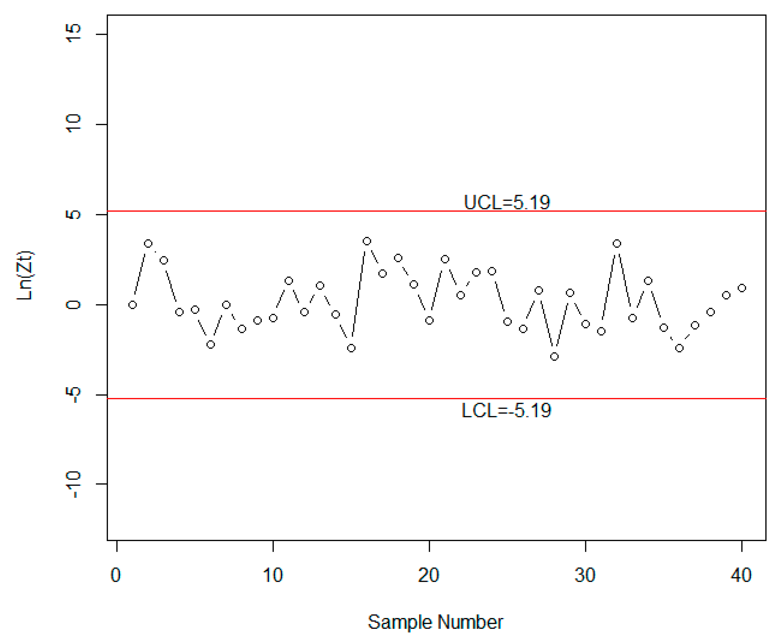
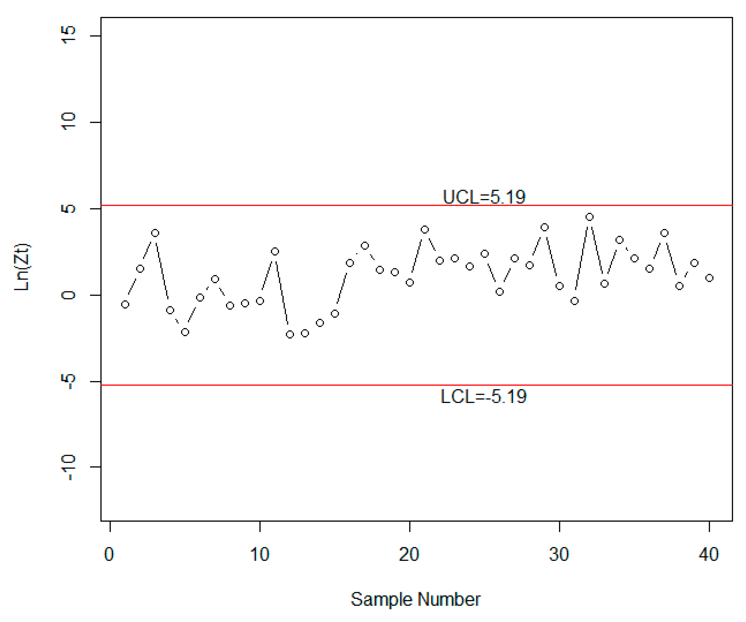
Control charts are used for monitoring the process for unusual changes in the process. The proposed scheme has been developed for the efficient monitoring of the mean time of the process under uncertainty environment. The proposed control chart has been examined using the simulation data of the mean time between two events. The first 20 neutrosophic observations are generated from the neutrosophic gamma distribution with neutrosophic parameters = [3,5], = [1.95,2.05] and = [2,2.2]. The next 20 observations are generated from the same distribution with s = 1.50. The gamma distributed data is transformed into a neutrosophic normal distribution using the transformation . At these parameters, the tabulated value of . It is expected that the process will be out-of-control between 14th sample and 24th sample. We plotted the values of statistic on the control chart in Figure 1. From Figure 1, it is clear that the first shift is at the 38th sample. The values of are also calculated for Aslam et al. [63] and plotted in Figure 2. From Figure 2, we note no shift indication in the process. By comparing both control charts, it is concluded that the proposed control chart provides the values of NARL in indeterminacy interval and gives the quick indication about the shift in the process as compared to the existing sampling plan. A quick indication in the shift in the process helps industrial engineers to identify the cause of variation which resulted in minimizing the non-conforming items.
5. Real Example
The application of the proposed control will be given in the healthcare department. Healthcare practitioners are interested in applying the proposed control chart for the monitoring of urinary tract infections (UTI) among male patients in a large hospital. A similar study was done by Santiago and Smith [64] and Aslam et al. [63] using classical statistics. The UTIs data is measured with the help of measurement devices. Therefore, there is a chance that observations are more fuzzy or imprecise. Under this uncertainty situation, the application of the existing control chart under classical statistics may mislead healthcare practitioners in monitoring the UTIs. Therefore, the proposed control chart is quite reasonable to apply for the monitoring of the UTIs infection. The neutrosophic data, which follows the gamma distribution with and is reported in Table 6.
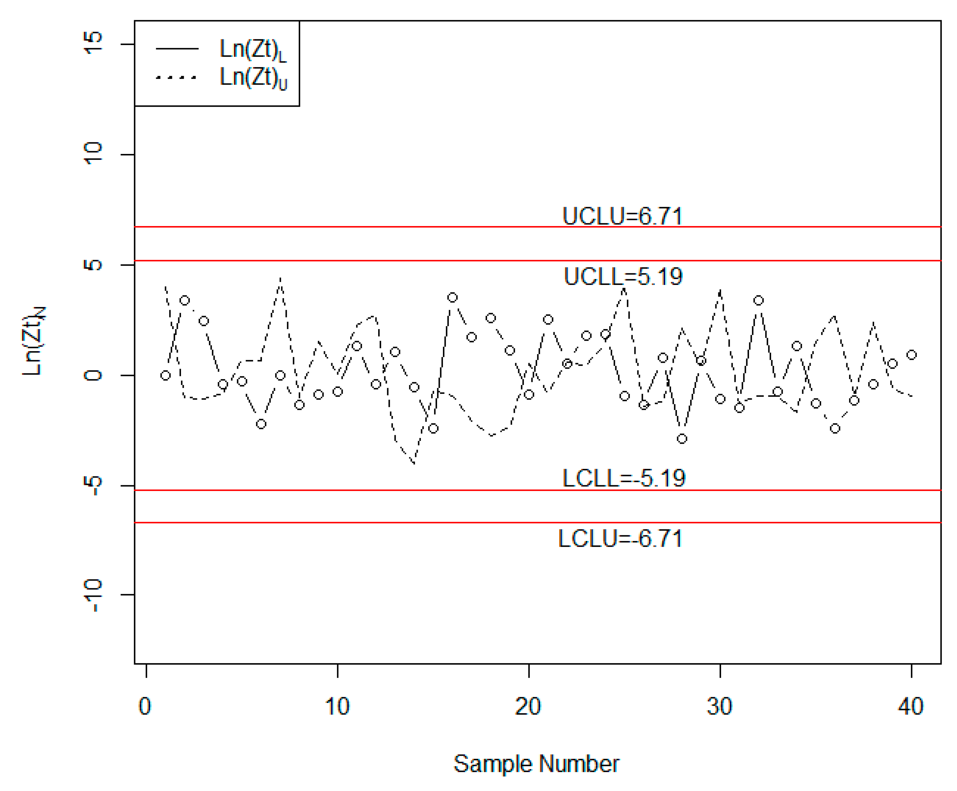
The control limits are calculated as follows: ; and ; . We set the initial value of and . As, which yield . The values of neutrosophic statistic are plotted in Figure 3. From Figure 3, we note although the process is an in-control state, the 16th sample and 33rd sample are near the control limits which indicate some issue in the process. The values of under classical statistics are also plotted in Figure 4. From Figure 4, it can be seen that only one point is near to control limit. By comparing both charts, it is concluded that the proposed control chart indicates that there is some issue in the process which should be identified. Therefore, the proposed control is more beneficial to be applied for the monitoring of UTIs inspection among male patients.
6. Conclusions
In this article, a control chart for the belief statistic under the gamma distribution has been presented when the interested quality characteristics of the process are imprecise, incomplete and vague. Although there are numerous techniques available in the literature like the fuzzy logic the proposed scheme is effective in dealing with vague information. The control limits have been determined for different settings of the parameters and different levels of process shifts. In this paper, the average run lengths for many settings of the proposed technique have been tabulated. The comparison of the proposed chart with the existing chart for different process shifts have been tested and it has been observed that the proposed chart is an effective addition in the toolkit of the quality control experts. We conclude that the proposed control is more robustness in detecting cause of variation in the process than the chart under classical statistics in uncertainty. The proposed chart can further be extended for other probability distributions, see, for example, references [65] and [66], particularly for the multivariate case.
Author Contributions
M.A.; R.A.R.B., N.K., and M.A. conceived and designed the experiments; M.A. and N.K. performed the experiments; M.A. and N.K. analyzed the data; M.A. contributed reagents/materials/analysis tools; M.A. wrote the paper.
Funding
This work was supported by the Deanship of Scientific Research (DSR), King Abdulaziz University, Jeddah, under grant No. (130-107-D1440). The author, therefore, gratefully acknowledge the DSR technical and financial support.
Acknowledgments
The authors are deeply thankful to the editor and reviewers for their valuable suggestions to improve the quality of this manuscript.
Conflicts of Interest
The authors declare no conflict of interest regarding this paper.
References
- Gülbay, M.; Kahraman, C.; Ruan, D. α-Cut fuzzy control charts for linguistic data. Int. J. Intell. Syst. 2004, 19, 1173–1195. [Google Scholar] [CrossRef]
- Demirli, K.; Vijayakumar, S. Fuzzy logic based assignable cause diagnosis using control chart patterns. Inf. Sci. 2010, 180, 3258–3272. [Google Scholar] [CrossRef]
- Montgomery, C.D. Introduction to Statistical Quality Control, 6th ed.; John Wiley & Sons, Inc.: New York, NY, USA, 2009. [Google Scholar]
- Cheng, C.-B. Fuzzy process control: Construction of control charts with fuzzy numbers. Fuzzy Sets Syst. 2005, 154, 287–303. [Google Scholar] [CrossRef]
- Gülbay, M.; Kahraman, C. An alternative approach to fuzzy control charts: Direct fuzzy approach. Inf. Sci. 2007, 177, 1463–1480. [Google Scholar] [CrossRef]
- Fallah Nezhad, M.S.; Akhavan Niaki, S.T. A new monitoring design for uni-variate statistical quality control charts. Inf. Sci. 2010, 180, 1051–1059. [Google Scholar] [CrossRef]
- Aksoy, H. Use of gamma distribution in hydrological analysis. Turk. J. Eng. Environ. Sci. 2000, 24, 419–428. [Google Scholar]
- Zhang, C.; Zhang, C.W.; Xie, M.; Liu, J.Y.; Goh, T.N. A control chart for the Gamma distribution as a model of time between events. Int. J. Prod. Res. 2007, 45, 5649–5666. [Google Scholar] [CrossRef]
- Aslam, M.; Arif, O.-H.; Jun, C.-H. A Control Chart for Gamma Distribution using Multiple Dependent State Sampling. Ind. Eng. Manag. Syst. 2017, 16, 109–117. [Google Scholar] [CrossRef] [Green Version]
- Chen, F.; Yeh, C.-H. Economic statistical design of non-uniform sampling scheme X bar control charts under non-normality and Gamma shock using genetic algorithm. Expert Syst. Appl. 2009, 36, 9488–9497. [Google Scholar] [CrossRef]
- Al-Oraini, H.A.; Rahim, M. Economic statistical design of X control charts for systems with Gamma (λ, 2) in-control times. Comput. Ind. Eng. 2002, 43, 645–654. [Google Scholar] [CrossRef]
- Bhaumik, D.K.; Gibbons, R.D. One-sided approximate prediction intervals for at least p of m observations from a gamma population at each of r locations. Technometrics 2006, 48, 112–119. [Google Scholar] [CrossRef]
- Khan, N.; Aslam, M.; Ahmad, L.; Jun, C.H. A Control Chart for Gamma Distributed Variables Using Repetitive Sampling Scheme. Pak. J. Stat. Oper. Res. 2017, 13, 47–61. [Google Scholar] [CrossRef]
- Kaya, I.; Erdoğan, M.; Yıldız, C. Analysis and control of variability by using fuzzy individual control charts. Appl. Soft Comput. 2017, 51, 370–381. [Google Scholar] [CrossRef]
- Smarandache, F. Neutrosophic logic-generalization of the intuitionistic fuzzy logic. arXiv, 2003; arXiv:math/0303009. [Google Scholar]
- Şentürk, S.; Erginel, N.; Kaya, İ.; Kahraman, C. Fuzzy exponentially weighted moving average control chart for univariate data with a real case application. Appl. Soft Comput. 2014, 22, 1–10. [Google Scholar] [CrossRef]
- Zadeh, L.A. Fuzzy sets. Inf. Control 1965, 8, 338–353. [Google Scholar] [CrossRef] [Green Version]
- Wang, J.-H.; Raz, T. On the construction of control charts using linguistic variables. Int. J. Prod. Res. 1990, 28, 477–487. [Google Scholar] [CrossRef]
- Raz, T.; Wang, J.-H. Probabilistic and membership approaches in the construction of control charts for linguistic data. Prod. Plan. Control 1990, 1, 147–157. [Google Scholar] [CrossRef]
- Taleb, H.; Limam, M. On fuzzy and probabilistic control charts. Int. J. Prod. Res. 2002, 40, 2849–2863. [Google Scholar] [CrossRef]
- Kanagawa, A.; Tamaki, F.; Ohta, H. Control charts for process average and variability based on linguistic data. Int. J. Prod. Res. 1993, 31, 913–922. [Google Scholar] [CrossRef]
- Erginel, N.; Sentürk, S.; Kahraman, C.; Kaya, I. Evaluating the packing process in food industry using fuzzy and [stilde] control charts. Int. J. Comput. Intell. Syst. 2011, 4, 509–520. [Google Scholar] [CrossRef]
- El-Shal, S.M.; Morris, A.S. A fuzzy rule-based algorithm to improve the performance of statistical process control in quality systems. J. Intell. Fuzzy Syst. 2000, 9, 207–223. [Google Scholar]
- Rowlands, H.; Wang, L.R. An approach of fuzzy logic evaluation and control in SPC. Qual. Reliab. Eng. Int. 2000, 16, 91–98. [Google Scholar] [CrossRef]
- Aslam, M. A New Sampling Plan Using Neutrosophic Process Loss Consideration. Symmetry 2018, 10, 132. [Google Scholar] [CrossRef]
- Senturk, S.; Erginel, N. Development of fuzzy and control charts using α-cuts. Inf. Sci. 2009, 179, 1542–1551. [Google Scholar] [CrossRef]
- Sentürk, S. Fuzzy regression control chart based on α-cut approximation. Int. J. Comput. Intell. Syst. 2010, 3, 123–140. [Google Scholar] [CrossRef]
- Kaya, İ.; Kahraman, C. Process capability analyses based on fuzzy measurements and fuzzy control charts. Expert Syst. Appl. 2011, 38, 3172–3184. [Google Scholar] [CrossRef]
- Broumi, S.; Smarandache, F. Correlation coefficient of interval neutrosophic set. In Applied Mechanics and Materials; Trans Tech Publication: Stafa-Zurich, Switzerland, 2013; pp. 511–517. [Google Scholar]
- Smarandache, F. Neutrosophic Logic-A Generalization of the Intuitionistic Fuzzy Logic. Multispace Multistruct. Neutrosophic Transdiscipl. 2010, 4, 396. [Google Scholar] [CrossRef]
- Smarandache, F. Neutrosophy: Neutrosophic Probability, Set, and Logic: Analytic Synthesis & Synthetic Analysis; American Research Press: Rehoboth, DE, USA, 1998; p. 105. [Google Scholar]
- Smarandache, F. Introduction to Neutrosophic Statistics; Infinite Study: Hollywood, FL, USA, 2014. [Google Scholar]
- Chen, J.; Ye, J.; Du, S. Scale effect and anisotropy analyzed for neutrosophic numbers of rock joint roughness coefficient based on neutrosophic statistics. Symmetry 2017, 9, 208. [Google Scholar] [CrossRef]
- Chen, J.; Ye, J.; Du, S.; Yong, R. Expressions of rock joint roughness coefficient using neutrosophic interval statistical numbers. Symmetry 2017, 9, 123. [Google Scholar] [CrossRef]
- Aslam, M. A New Failure-Censored Reliability Test Using Neutrosophic Statistical Interval Method. Int. J. Fuzzy Syst. 2019, 1–7. [Google Scholar] [CrossRef]
- Aslam, M. Design of Sampling Plan for Exponential Distribution under Neutrosophic Statistical Interval Method. IEEE Access 2018, 6, 64153–64158. [Google Scholar] [CrossRef]
- Aslam, M. A new attribute sampling plan using neutrosophic statistical interval method. Complex Intell. Syst. 2019, 1–6. [Google Scholar] [CrossRef]
- Aslam, M.; Bantan, R.A.; Khan, N. Design of a New Attribute Control Chart Under Neutrosophic Statistics. Int. J. Fuzzy Syst. 2019, 21, 433–440. [Google Scholar] [CrossRef]
- Aslam, M.; Khan, N.; Khan, M. Monitoring the Variability in the Process Using Neutrosophic Statistical Interval Method. Symmetry 2018, 10, 562. [Google Scholar] [CrossRef]
- Aslam, M.; Bantan, R.A.; Khan, N. Design of a Control Chart for Gamma Distributed Variables under the Indeterminate Environment. IEEE Access 2019, 7, 8858–8864. [Google Scholar] [CrossRef]
- Aslam, M. Product Acceptance Determination with Measurement Error Using the Neutrosophic Statistics. Adv. Fuzzy Syst. 2019, 2019, 8953051. [Google Scholar] [CrossRef]
- Aslam, M.; Arif, O. Testing of Grouped Product for the Weibull Distribution Using Neutrosophic Statistics. Symmetry 2018, 10, 403. [Google Scholar] [CrossRef]
- Aslam, M.; Raza, M.A. Design of New Sampling Plans for Multiple Manufacturing Lines Under Uncertainty. Int. J. Fuzzy Syst. 2019, 21, 978–992. [Google Scholar] [CrossRef]
- Peng, X.; Dai, J. A bibliometric analysis of neutrosophic set: Two decades review from 1998 to 2017. Artif. Intell. Rev. 2018, 1–57. [Google Scholar] [CrossRef]
- Peng, X.; Dai, J. Approaches to single-valued neutrosophic MADM based on MABAC, TOPSIS and new similarity measure with score function. Neural Comput. Appl. 2018, 29, 939–954. [Google Scholar] [CrossRef]
- Smarandache, F. Neutrosophic set-a generalization of the intuitionistic fuzzy set. J. Def. Resour. Manag. 2010, 1, 107. [Google Scholar]
- Smarandache, F. A geometric interpretation of the neutrosophic set-A generalization of the intuitionistic fuzzy set. arXiv, 2004; arXiv:math/0404520. [Google Scholar]
- Smarandache, F. n-Valued Refined Neutrosophic Logic and Its Applications to Physics. Available online: https://arxiv.org/pdf/1407.104 (accessed on 12 March 2019).
- Rivieccio, U. Neutrosophic logics: Prospects and problems. Fuzzy Sets Syst. 2008, 159, 1860–1868. [Google Scholar] [CrossRef]
- Wang, H.; Smarandache, F.; Zhang, Y.; Sunderraman, R. Single Valued Neutrosophic Sets. Available online: fs.unm.edu/SingleValuedNeutrosophicSets.pdf (accessed on 12 March 2019).
- Wang, H.; Smarandache, F.; Sunderraman, R.; Zhang, Y.Q. Interval Neutrosophic Sets and Logic: Theory and Applications in Computing: Theory and Applications in Computing. Available online: https://arxiv.org/abs/cs/0505014 (accessed on 12 March 2019).
- Gao, Z.; Cecati, C.; Ding, S.X. A survey of fault diagnosis and fault-tolerant techniques—Part II: Fault diagnosis with knowledge-based and hybrid/active approaches. IEEE Trans. Ind. Electron. 2015, 62, 3768–3774. [Google Scholar] [CrossRef]
- Wilson, E.B.; Hilferty, M.M. The distribution of chi-square. Proc. Natl. Acad. Sci. USA 1931, 17, 684–688. [Google Scholar] [CrossRef]
- Ahmad, L.; Aslam, M.; Jun, C.-H. Designing of X-bar control charts based on process capability index using repetitive sampling. Trans. Inst. Meas. Control 2014, 36, 367–374. [Google Scholar] [CrossRef]
- Knoth, S. Accurate ARL Calculation for EWMA Control Charts Monitoring Normal Mean and Variance Simultaneously. Seq. Anal. 2007, 26, 251–263. [Google Scholar] [CrossRef]
- Li, Z.H.; Zou, C.; Gong, Z.; Wang, Z. The computation of average run length and average time to signal: An overview. J. Stat. Comput. Simul. 2014, 84, 1779–1802. [Google Scholar] [CrossRef]
- Lee, M.; Khoo, M.B. Optimal statistical design of a multivariate EWMA chart based on ARL and MRL. Commun. Stat. Simul. Comput. 2006, 35, 831–847. [Google Scholar] [CrossRef]
- Phanyaem, S.; Areepong, Y.; Sukparungsee, S. Numerical Integration of Average Run Length of CUSUM Control Chart for ARMA Process. Int. J. Appl. Phys. Math. 2014, 4, 232–235. [Google Scholar] [CrossRef]
- Busaba, J.; Sukparungsee, S.; Areepong, Y. Numerical approximations of average run length for AR (1) on exponential CUSUM. Comput. Sci. Telecommun. 2012, 19, 23. [Google Scholar]
- Aslam, M.; Khan, N.; Ahmad, L.; Jun, C.H.; Hussain, J. A mixed control chart using process capability index. Seq. Anal. 2017, 36, 278–289. [Google Scholar] [CrossRef]
- Ahmad, L.; Aslam, M.; Khan, N.; Jun, C.H. Double moving average control chart for exponential distributed life using EWMA. In AIP Conference Proceedings; AIP Publishing: New York, NY, USA, 2017. [Google Scholar]
- Ahmad, L.; Aslam, M.; Jun, C.-H. Coal Quality Monitoring With Improved Control Charts. Eur. J. Sci. Res. 2014, 125, 427–434. [Google Scholar]
- Aslam, M.; Khan, N.; Jun, C.-H. A control chart using belief information for a gamma distribution. Oper. Res. Decis. 2016, 26, 5–19. [Google Scholar]
- Santiago, E.; Smith, J. Control charts based on the exponential distribution: Adapting runs rules for the t chart. Qual. Eng. 2013, 25, 85–96. [Google Scholar] [CrossRef]
- Smarandache, F. Introduction to Neutrosophic Measure, Neutrosophic Integral, and Neutrosophic Probability. Available online: https://arxiv.org/abs/1311.7139 (accessed on 12 March 2019).
- Smarandache, F. Neutrosophic Precalculus and Neutrosophic Calculus: Neutrosophic Applications. Available online: https://arxiv.org/pdf/1509.07723 (accessed on 12 March 2019).
Figure 1.
The proposed chart for the simulated data.

Figure 2.
The existing chart for the simulated data.

Figure 3.
The proposed chart for the real data.

Figure 4.
The existing chart for the real data.


Table 1.
The values of neutrosophic average run length (NARL) when and .
| [2.8071,2.8141] | [2.9354,2.9416] | [3.0003,3.0012] | |
| s | NARL | ||
| 4.00 | [1.28,1.06] | [1.32,1.07] | [1.34,1.07] |
| 3.00 | [1.76,1.24] | [1.88,1.28] | [1.95,1.31] |
| 2.80 | [1.98,1.34] | [2.13,1.40] | [2.22,1.43] |
| 2.50 | [2.50,1.58] | [2.75,1.68] | [2.89,1.73] |
| 2.25 | [3.27,1.97] | [3.67,2.13] | [3.91,2.22] |
| 2.00 | [4.75,2.74] | [5.48,3.05] | [5.92,3.22] |
| 1.90 | [5.74,3.28] | [6.71,3.70] | [7.29,3.93] |
| 1.80 | [7.13,4.05] | [8.47,4.66] | [9.28,4.98] |
| 1.70 | [9.18,5.24] | [11.1,6.12] | [12.26,6.61] |
| 1.60 | [12.32,7.12] | [15.19,8.51] | [16.96,9.28] |
| 1.50 | [17.4,10.34] | [21.93,12.67] | [24.76,13.98] |
| 1.40 | [26.08,16.27] | [33.74,20.51] | [38.61,22.94] |
| 1.30 | [41.89,28.25] | [55.90,36.86] | [64.99,41.90] |
| 1.20 | [72.12,54.92] | [99.88,74.68] | [118.35,86.58] |
| 1.10 | [127.96,115.71] | [185.0,165.6] | [224.15,196.69] |
| 1.00 | [200.02,204.41] | [300.17,306.26] | [370.82,371.83] |
| 0.80 | [152.58,98.67] | [227.95,143.72] | [281.15,172.31] |
| 0.75 | [119.34,67.59] | [177.29,97.32] | [218.11,116.09] |
| 0.70 | [90.73,45.44] | [134.07,64.61] | [164.56,76.64] |
| 0.60 | [49.26,19.71] | [71.88,27.17] | [87.73,31.78] |
| 0.50 | [24.63,8.22] | [35.26,10.86] | [42.65,12.45] |
| 0.40 | [11.21,3.44] | [15.56,4.26] | [18.55,4.75] |
| 0.30 | [4.64,1.60] | [6.10,1.82] | [7.09,1.95] |
| 0.25 | [2.91,1.22] | [3.68,1.32] | [4.19,1.37] |
| 0.15 | [1.27,1.00] | [1.4,1.01] | [1.49,1.01] |
| 0.10 | [1.03,1.00] | [1.05,1.00] | [1.07,1.00] |
| 0.05 | [1.00,1.00] | [1.00,1.00] | [1.00,1.00] |
Table 2.
The values of NARL when and .
| [2.8071,2.8164] | [2.9354,2.9436] | [2.9997,3.007] | |
| s | NARL | ||
| 4.00 | [1.01,1] | [1.01,1] | [1.01,1] |
| 3.00 | [1.07,1.02] | [1.08,1.03] | [1.09,1.03] |
| 2.80 | [1.11,1.04] | [1.13,1.05] | [1.14,1.05] |
| 2.50 | [1.23,1.1] | [1.27,1.12] | [1.29,1.13] |
| 2.25 | [1.43,1.22] | [1.5,1.26] | [1.54,1.28] |
| 2.00 | [1.86,1.5] | [2.01,1.59] | [2.1,1.64] |
| 1.90 | [2.17,1.71] | [2.38,1.83] | [2.5,1.9] |
| 1.80 | [2.63,2.02] | [2.93,2.21] | [3.1,2.31] |
| 1.70 | [3.34,2.52] | [3.8,2.81] | [4.07,2.97] |
| 1.60 | [4.51,3.36] | [5.25,3.83] | [5.69,4.1] |
| 1.50 | [6.58,4.88] | [7.87,5.72] | [8.64,6.22] |
| 1.40 | [10.58,7.92] | [13.06,9.6] | [14.57,10.61] |
| 1.30 | [19.27,14.85] | [24.68,18.73] | [28.06,21.11] |
| 1.20 | [40.86,33.47] | [54.79,44.29] | [63.76,51.16] |
| 1.10 | [99.7,91.45] | [141.65,128.72] | [169.75,153.39] |
| 1.00 | [200.01,205.94] | [300.2,308.26] | [370.01,379.03] |
| 0.80 | [63.82,47.69] | [91.14,66.87] | [109.64,79.63] |
| 0.75 | [39.6,27.68] | [55.57,37.96] | [66.28,44.72] |
| 0.70 | [24.4,16.13] | [33.57,21.58] | [39.66,25.12] |
| 0.60 | [9.26,5.74] | [12.14,7.23] | [14.01,8.17] |
| 0.50 | [3.69,2.34] | [4.54,2.74] | [5.07,2.98] |
| 0.40 | [1.71,1.27] | [1.94,1.36] | [2.08,1.42] |
| 0.30 | [1.09,1.01] | [1.14,1.02] | [1.16,1.03] |
| 0.25 | [1.02,1.00] | [1.03,1.00] | [1.03,1.00] |
| 0.15 | [1.00,1.00] | [1.00,1.00] | [1.00,1.00] |
| 0.10 | [1.00,1.00] | [1.00,1.00] | [1.00,1.00] |
| 0.05 | [1.00,1.00] | [1.00,1.00] | [1.00,1.00] |
Table 3.
The values of NARL when and .
| [2.8071,2.8142] | [2.9352,2.9392] | [2.9997,3.0056] | |
| s | NARL | ||
| 4.00 | [2.09,1.4] | [2.24,1.45] | [2.32,1.49] |
| 3.00 | [3.34,2.02] | [3.71,2.17] | [3.92,2.26] |
| 2.80 | [3.86,2.29] | [4.33,2.49] | [4.61,2.61] |
| 2.50 | [5.04,2.93] | [5.78,3.25] | [6.21,3.43] |
| 2.25 | [6.74,3.88] | [7.88,4.38] | [8.56,4.69] |
| 2.00 | [9.78,5.66] | [11.74,6.58] | [12.92,7.15] |
| 1.90 | [11.71,6.84] | [14.24,8.05] | [15.76,8.81] |
| 1.80 | [14.33,8.5] | [17.66,10.15] | [19.69,11.19] |
| 1.70 | [17.99,10.91] | [22.52,13.24] | [25.31,14.73] |
| 1.60 | [23.25,14.56] | [29.63,18] | [33.6,20.23] |
| 1.50 | [31.1,20.36] | [40.43,25.71] | [46.32,29.23] |
| 1.40 | [43.21,30.06] | [57.47,38.92] | [66.63,44.84] |
| 1.30 | [62.46,47.23] | [85.32,62.95] | [100.27,73.68] |
| 1.20 | [93.37,78.73] | [131.5,108.66] | [156.99,129.57] |
| 1.10 | [140.64,134.1] | [204.74,192.56] | [248.65,234.62] |
| 1.00 | [200.02,204.48] | [300.01,303.91] | [370.04,377.32] |
| 0.80 | [238.37,175.18] | [365.34,260.87] | [455.85,324.45] |
| 0.75 | [220.33,142.4] | [338.02,211.22] | [422.1,262.24] |
| 0.70 | [197.09,112.31] | [302.88,166.02] | [378.67,205.82] |
| 0.60 | [147.18,65.42] | [227.51,95.98] | [285.52,118.6] |
| 0.50 | [101.86,34.98] | [158.66,50.71] | [200.09,62.32] |
| 0.40 | [64.33,16.86] | [100.95,23.93] | [127.95,29.12] |
| 0.30 | [35.38,7.15] | [55.76,9.77] | [70.97,11.66] |
| 0.25 | [24.24,4.43] | [38.16,5.86] | [48.62,6.88] |
| 0.15 | [8.68,1.64] | [13.36,1.93] | [16.9,2.13] |
| 0.10 | [4.15,1.12] | [6.10,1.20] | [7.59,1.26] |
| 0.05 | [1.60,1.00] | [2.05,1.00] | [2.39,1.00] |
Table 4.
The values of NARL when and .
| [2.8071,2.8145] | [2.9354,2.9399] | [2.9998,3.0019] | |
| s | NARL | ||
| 4.00 | [1.18,1.07] | [1.21,1.08] | [1.22,1.08] |
| 3.00 | [1.55,1.27] | [1.64,1.32] | [1.68,1.34] |
| 2.80 | [1.72,1.38] | [1.83,1.44] | [1.90,1.47] |
| 2.50 | [2.13,1.64] | [2.32,1.74] | [2.42,1.80] |
| 2.25 | [2.76,2.05] | [3.06,2.22] | [3.24,2.32] |
| 2.00 | [3.97,2.87] | [4.53,3.20] | [4.86,3.39] |
| 1.90 | [4.78,3.43] | [5.54,3.88] | [5.98,4.14] |
| 1.80 | [5.95,4.25] | [7.00,4.89] | [7.62,5.25] |
| 1.70 | [7.68,5.50] | [9.20,6.43] | [10.10,6.97] |
| 1.60 | [10.37,7.48] | [12.67,8.94] | [14.06,9.79] |
| 1.50 | [14.79,10.84] | [18.49,13.27] | [20.77,14.71] |
| 1.40 | [22.54,17] | [28.94,21.4] | [32.96,24.07] |
| 1.30 | [37.13,29.36] | [49.22,38.19] | [56.97,43.67] |
| 1.20 | [66.38,56.51] | [91.46,76.54] | [107.95,89.33] |
| 1.10 | [123.82,117.26] | [178.57,166.92] | [215.76,199.71] |
| 1.00 | [200.02,204.72] | [300.15,304.57] | [370.2,372.66] |
| 0.80 | [133.37,103.02] | [197.81,149.39] | [242.69,180.6] |
| 0.75 | [100.03,71.35] | [147.26,102.35] | [180.06,123.11] |
| 0.70 | [73.11,48.45] | [106.83,68.69] | [130.19,82.17] |
| 0.60 | [36.85,21.38] | [52.88,29.45] | [63.9,34.75] |
| 0.50 | [17.23,9.02] | [24.08,11.93] | [28.73,13.8] |
| 0.40 | [7.48,3.76] | [10.03,4.69] | [11.73,5.28] |
| 0.30 | [3.10,1.71] | [3.89,1.96] | [4.40,2.11] |
| 0.25 | [2.02,1.28] | [2.42,1.39] | [2.67,1.46] |
| 0.15 | [1.09,1.00] | [1.14,1.01] | [1.18,1.01] |
| 0.10 | [1.00,1.00] | [1.01,1.00] | [1.01,1.00] |
| 0.05 | [1.00,1.00] | [1.00,1.00] | [1.00,1.00] |
Table 5.
Comparison of average run length values at different levels of shift when a = 0.95 and k = 8.
Table 5.
Comparison of average run length values at different levels of shift when a = 0.95 and k = 8.
| s | Control Chart [63] | The Proposed Chart | ||||
|---|---|---|---|---|---|---|
| ARLs | NARL | |||||
| 4.00 | 1.178764 | 1.206864 | 1.2224 | [1.18,1.07] | [1.21,1.08] | [1.22,1.08] |
| 3.00 | 1.550192 | 1.635354 | 1.68279 | [1.55,1.27] | [1.64,1.32] | [1.68,1.34] |
| 2.80 | 1.720708 | 1.833704 | 1.896919 | [1.72,1.38] | [1.83,1.44] | [1.90,1.47] |
| 2.50 | 2.133142 | 2.317927 | 2.422306 | [2.13,1.64] | [2.32,1.74] | [2.42,1.80] |
| 2.25 | 2.757243 | 3.061253 | 3.23504 | [2.76,2.05] | [3.06,2.22] | [3.24,2.32] |
| 2.00 | 3.967114 | 4.530703 | 4.858373 | [3.97,2.87] | [4.53,3.20] | [4.86,3.39] |
| 1.90 | 4.783924 | 5.539304 | 5.982269 | [4.78,3.43] | [5.54,3.88] | [5.98,4.14] |
| 1.80 | 5.950011 | 6.99735 | 7.617622 | [5.95,4.25] | [7.00,4.89] | [7.62,5.25] |
| 1.70 | 7.680794 | 9.193211 | 10.09918 | [7.68,5.50] | [9.20,6.43] | [10.10,6.97] |
| 1.60 | 10.37155 | 12.66559 | 14.058 | [10.37,7.48] | [12.67,8.94] | [14.06,9.79] |
| 1.50 | 14.79182 | 18.4856 | 20.76225 | [14.79,10.84] | [18.49,13.27] | [20.77,14.71] |
| 1.40 | 22.53872 | 28.93451 | 32.94814 | [22.54,17] | [28.94,21.4] | [32.96,24.07] |
| 1.30 | 37.12749 | 49.20506 | 56.94885 | [37.13,29.36] | [49.22,38.19] | [56.97,43.67] |
| 1.20 | 66.37585 | 91.41983 | 107.9055 | [66.38,56.51] | [91.46,76.54] | [107.95,89.33] |
| 1.10 | 123.8084 | 178.4871 | 215.6592 | [123.82,117.26] | [178.57,166.92] | [215.76,199.71] |
| 1.00 | 200 | 300 | 370.0001 | [200.02,204.72] | [300.15,304.57] | [370.2,372.66] |
| 0.80 | 133.3607 | 197.7073 | 242.5684 | [133.37,103.02] | [197.81,149.39] | [242.69,180.6] |
| 0.75 | 100.0185 | 147.1854 | 179.9717 | [100.03,71.35] | [147.26,102.35] | [180.06,123.11] |
| 0.70 | 73.10437 | 106.7805 | 130.1201 | [73.11,48.45] | [106.83,68.69] | [130.19,82.17] |
| 0.60 | 36.84876 | 52.85517 | 63.86527 | [36.85,21.38] | [52.88,29.45] | [63.9,34.75] |
| 0.50 | 17.23191 | 24.06818 | 28.71763 | [17.23,9.02] | [24.08,11.93] | [28.73,13.8] |
| 0.40 | 7.479311 | 10.02559 | 11.72831 | [7.48,3.76] | [10.03,4.69] | [11.73,5.28] |
| 0.30 | 3.097514 | 3.884251 | 4.398122 | [3.10,1.71] | [3.89,1.96] | [4.40,2.11] |
| 0.25 | 2.023985 | 2.417816 | 2.672091 | [2.02,1.28] | [2.42,1.39] | [2.67,1.46] |
| 0.15 | 1.090389 | 1.144401 | 1.180756 | [1.09,1.00] | [1.14,1.01] | [1.18,1.01] |
| 0.10 | 1.003689 | 1.008166 | 1.011881 | [1.00,1.00] | [1.01,1.00] | [1.01,1.00] |
| 0.05 | 1.000 | 1.000 | 1.000001 | [1.00,1.00] | [1.00,1.00] | [1.00,1.00] |
Table 6.
The data for a real example.
| Sr. # | B(k) | z(k) | ln(zk) |
|---|---|---|---|
| 1 | [0.496,0.982] | [0.985,54.568] | [−0.015,3.999] |
| 2 | [0.968,0.261] | [30.555,0.353] | [3.42,−1.04] |
| 3 | [0.922,0.252] | [11.788,0.338] | [2.467,−1.086] |
| 4 | [0.403,0.290] | [0.675,0.408] | [−0.393,−0.897] |
| 5 | [0.432,0.654] | [0.761,1.891] | [−0.274,0.637] |
| 6 | [0.096,0.652] | [0.106,1.872] | [−2.247,0.627] |
| 7 | [0.490,0.988] | [0.962,83.351] | [−0.039,4.423] |
| 8 | [0.204,0.264] | [0.256,0.358] | [−1.363,−1.028] |
| 9 | [0.287,0.820] | [0.403,4.546] | [−0.908,1.514] |
| 10 | [0.325,0.519] | [0.481,1.078] | [−0.732,0.075] |
| 11 | [0.795,0.904] | [3.885,9.443] | [1.357,2.245] |
| 12 | [0.396,0.941] | [0.656,15.825] | [−0.421,2.762] |
| 13 | [0.740,0.049] | [2.843,0.051] | [1.045,−2.974] |
| 14 | [0.361,0.017] | [0.564,0.017] | [−0.572,−4.048] |
| 15 | [0.084,0.331] | [0.091,0.496] | [−2.393,−0.701] |
| 16 | [0.972,0.278] | [34.857,0.385] | [3.551,−0.956] |
| 17 | [0.849,0.109] | [5.611,0.122] | [1.725,−2.101] |
| 18 | [0.932,0.06] | [13.683,0.064] | [2.616,−2.75] |
| 19 | [0.752,0.086] | [3.028,0.094] | [1.108,−2.364] |
| 20 | [0.293,0.621] | [0.414,1.64] | [−0.883,0.495] |
| 21 | [0.924,0.304] | [12.2,0.436] | [2.501,−0.829] |
| 22 | [0.631,0.636] | [1.709,1.748] | [0.536,0.558] |
| 23 | [0.859,0.611] | [6.108,1.572] | [1.810,0.452] |
| 24 | [0.863,0.812] | [6.296,4.306] | [1.840,1.460] |
| 25 | [0.279,0.983] | [0.388,59.465] | [−0.947,4.085] |
| 26 | [0.208,0.191] | [0.263,0.236] | [−1.337,−1.445] |
| 27 | [0.691,0.232] | [2.236,0.303] | [0.805,−1.195] |
| 28 | [0.052,0.896] | [0.055,8.661] | [−2.908,2.159] |
| 29 | [0.659,0.608] | [1.936,1.551] | [0.660,0.439] |
| 30 | [0.252,0.981] | [0.337,50.315] | [−1.087,3.918] |
| 31 | [0.186,0.221] | [0.229,0.283] | [−1.475,−1.262] |
| 32 | [0.968,0.286] | [29.788,0.4] | [3.394,−0.916] |
| 33 | [0.324,0.279] | [0.479,0.387] | [−0.736,−0.95] |
| 34 | [0.791,0.157] | [3.78,0.186] | [1.33,−1.684] |
| 35 | [0.217,0.812] | [0.277,4.321] | [−1.284,1.464] |
| 36 | [0.08,0.942] | [0.086,16.316] | [−2.449,2.792] |
| 37 | [0.246,0.273] | [0.327,0.376] | [−1.119,−0.979] |
| 38 | [0.398,0.914] | [0.66,10.644] | [−0.415,2.365] |
| 39 | [0.625,0.358] | [1.665,0.557] | [0.51,−0.586] |
| 40 | [0.720,0.286] | [2.569,0.400] | [0.944,−0.916] |
© 2019 by the authors. Licensee MDPI, Basel, Switzerland. This article is an open access article distributed under the terms and conditions of the Creative Commons Attribution (CC BY) license (http://creativecommons.org/licenses/by/4.0/).
Share and Cite
MDPI and ACS Style
Aslam, M.; Bantan, R.A.R.; Khan, N. Monitoring the Process Based on Belief Statistic for Neutrosophic Gamma Distributed Product. Processes 2019, 7, 209. https://0-doi-org.brum.beds.ac.uk/10.3390/pr7040209
AMA Style
Aslam M, Bantan RAR, Khan N. Monitoring the Process Based on Belief Statistic for Neutrosophic Gamma Distributed Product. Processes. 2019; 7(4):209. https://0-doi-org.brum.beds.ac.uk/10.3390/pr7040209
Chicago/Turabian StyleAslam, Muhammad, Rashad A. R. Bantan, and Nasrullah Khan. 2019. "Monitoring the Process Based on Belief Statistic for Neutrosophic Gamma Distributed Product" Processes 7, no. 4: 209. https://0-doi-org.brum.beds.ac.uk/10.3390/pr7040209
Note that from the first issue of 2016, this journal uses article numbers instead of page numbers. See further details here.