Dynamic Flowsheet Model Development and Sensitivity Analysis of a Continuous Pharmaceutical Tablet Manufacturing Process Using the Wet Granulation Route

 , , ,
, , , 
Abstract
:
1. Introduction
Objectives
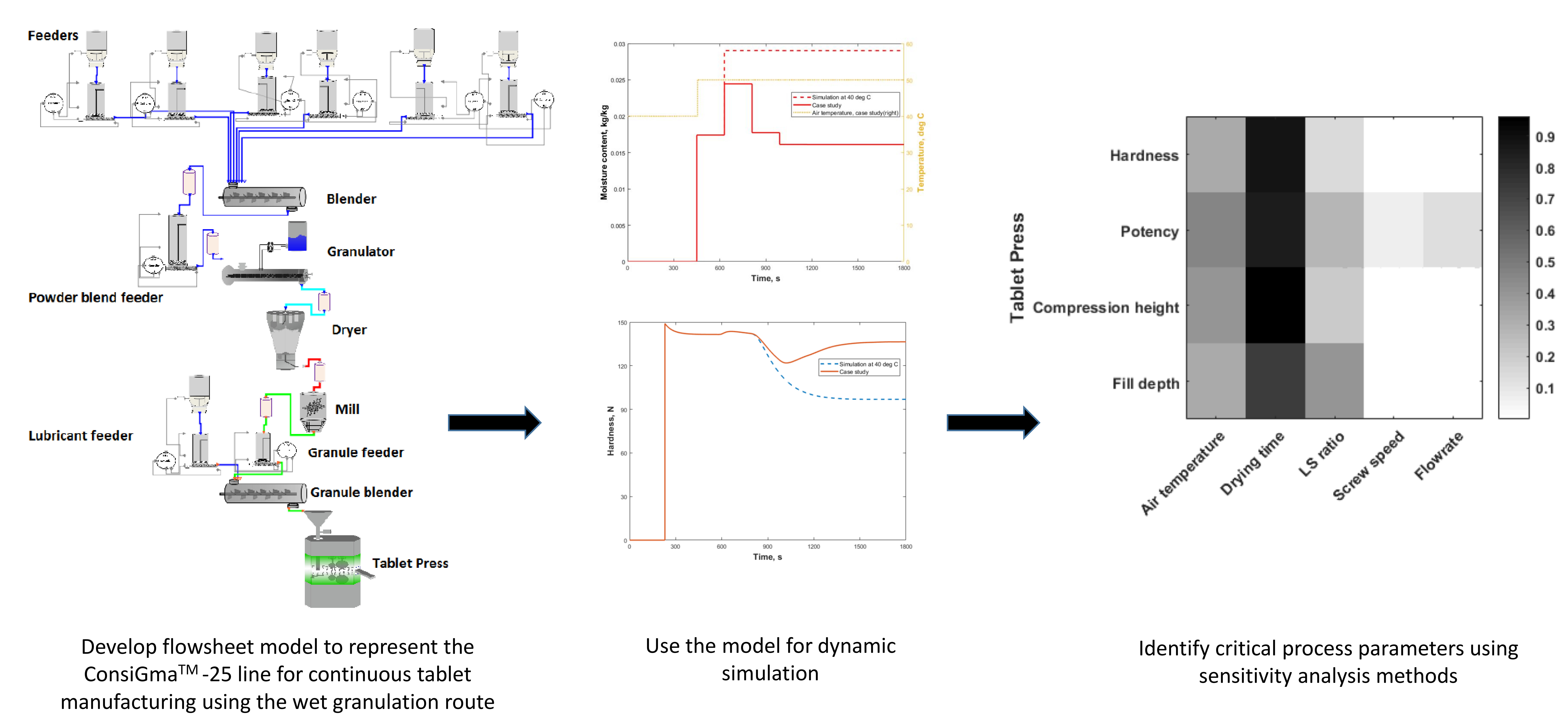
- Develop a flowsheet model approximating the ConsiGma-25 wet granulation manufacturing line;
- Demonstrate the use of the flowsheet model for simulating effects of disturbances in the continuous process;
- Identify critical process parameters (CPPs) affecting the properties of intermediate and final product.
2. Materials and Methods
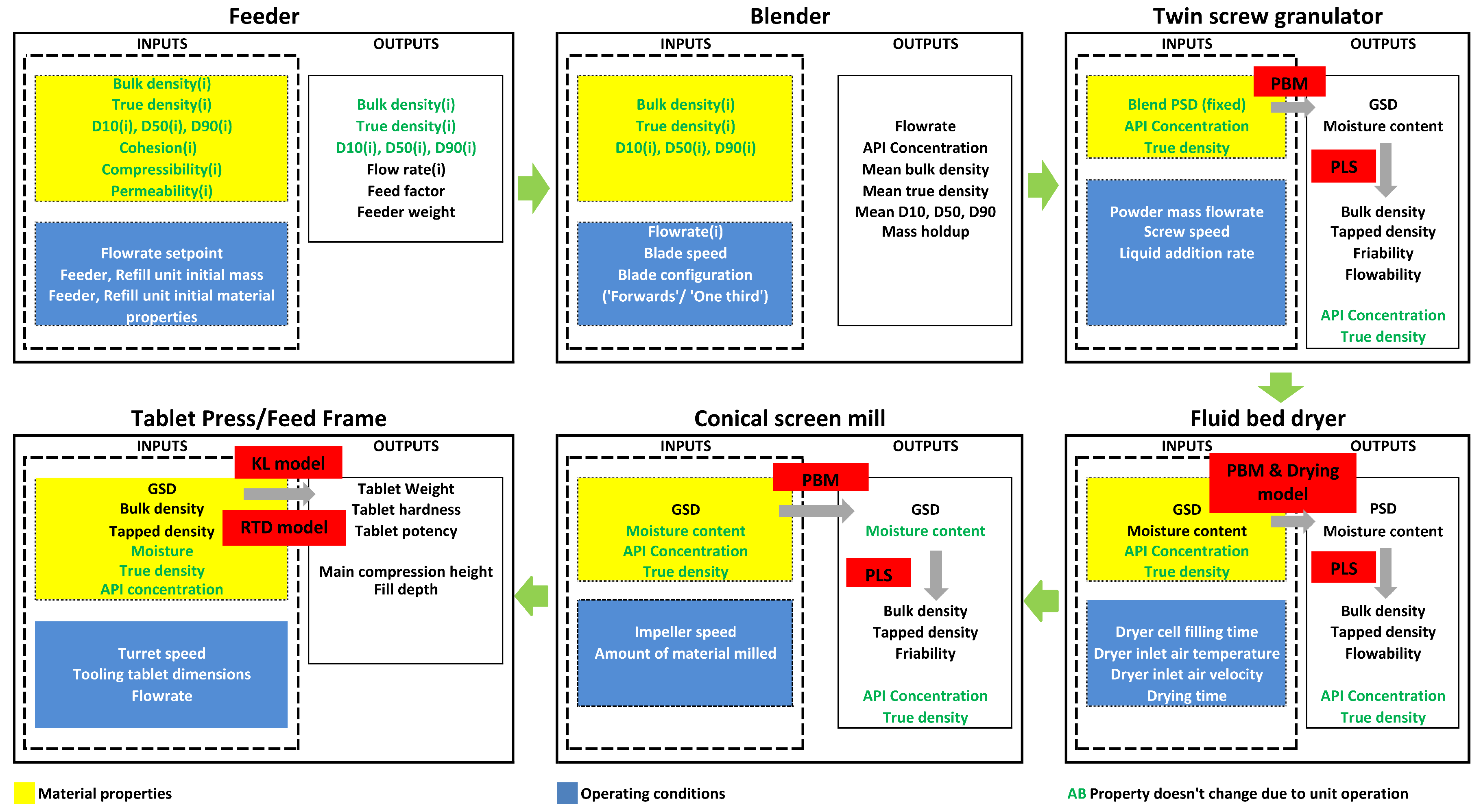
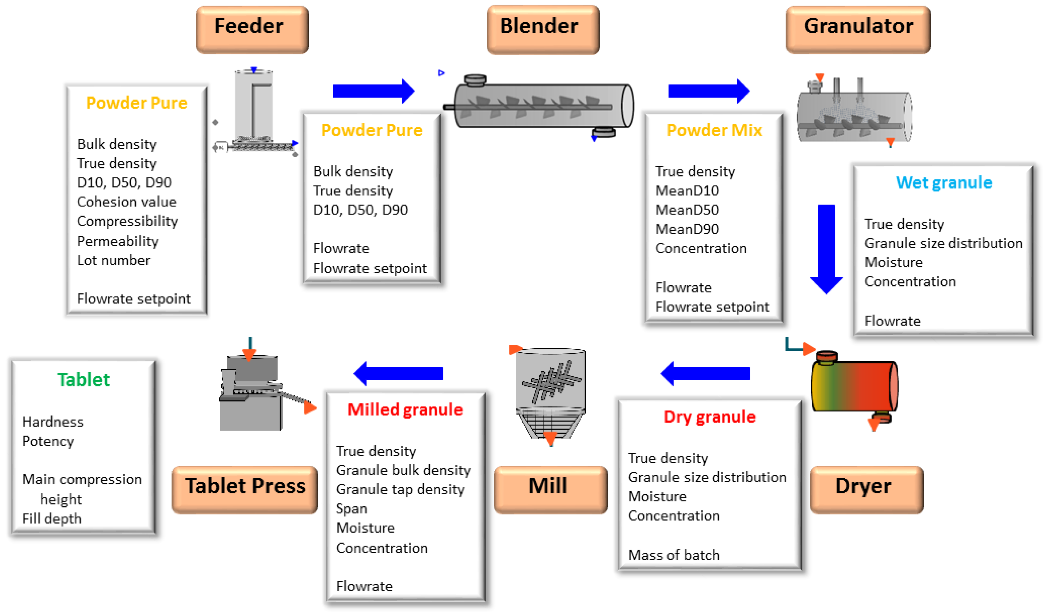
2.1. Flowsheet Modeling
2.1.1. Feeder
2.1.2. Blender
2.1.3. Twin-Screw Wet Granulator
2.1.4. Dryer
2.1.5. Mill
2.1.6. Tablet Press
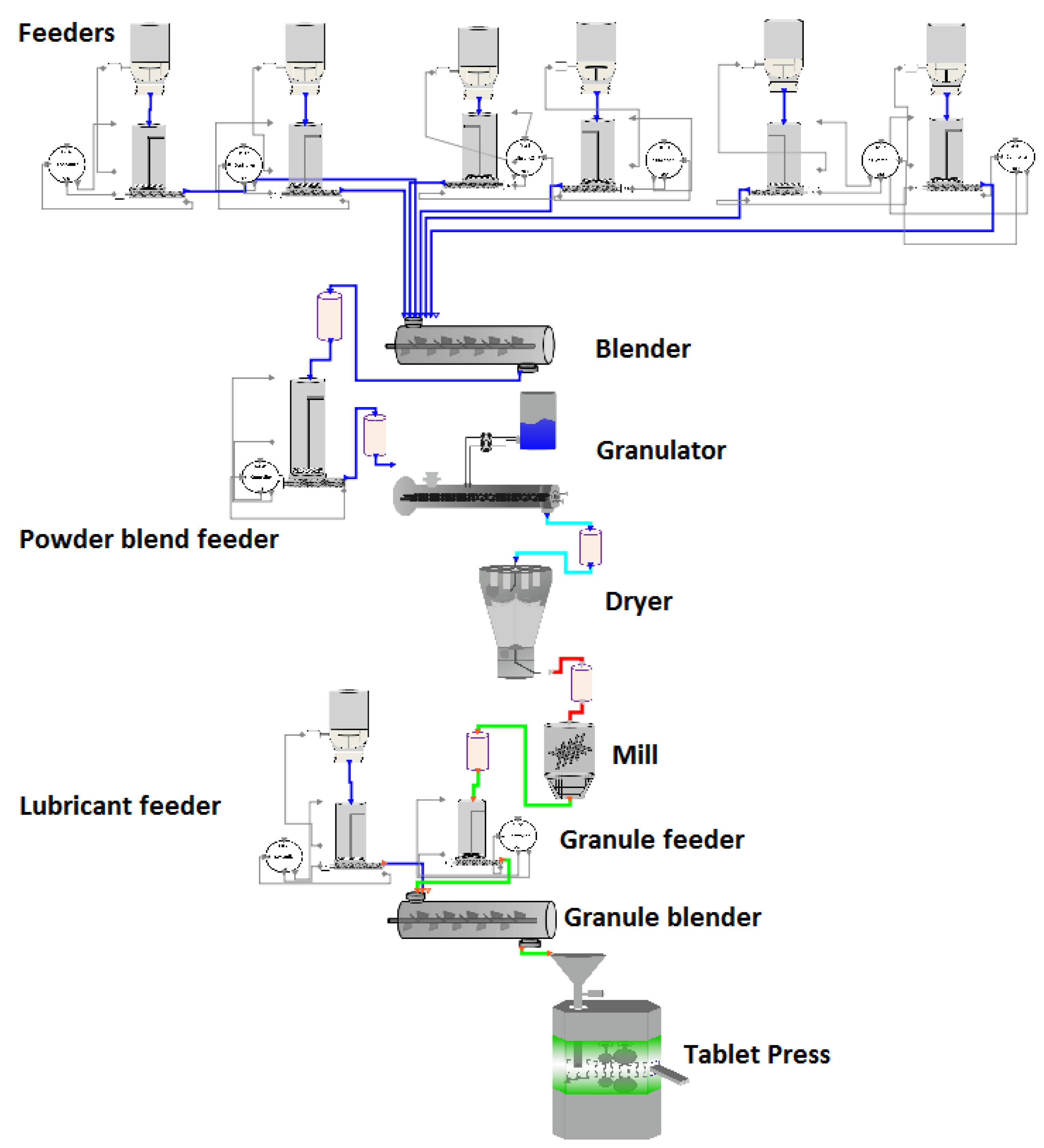
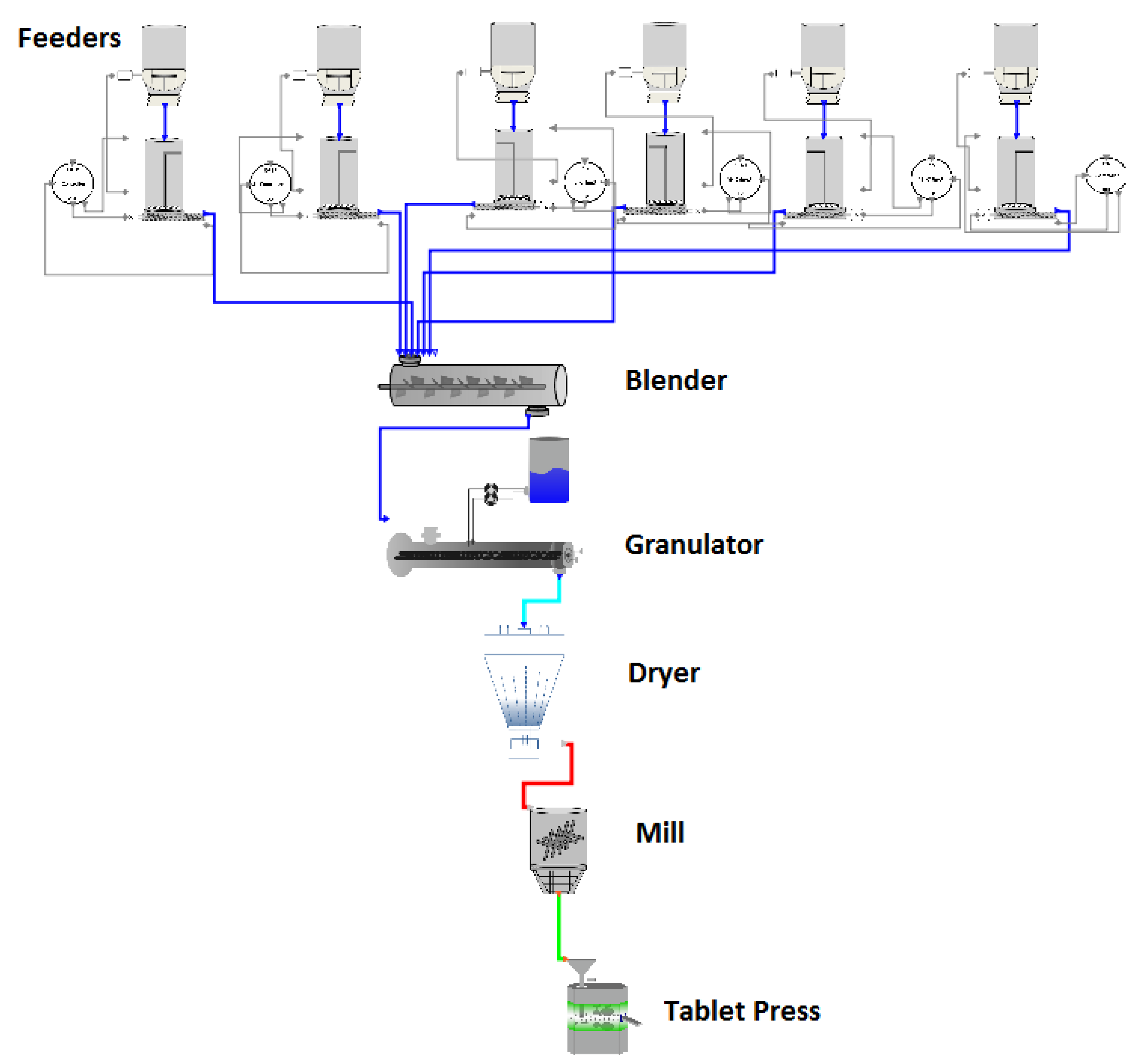
2.1.7. Overview
2.1.8. Intermediate Feeders, Blender, and Transfer Lines
2.2. Scenario Analysis
2.3. Sensitivity Analysis
2.3.1. Morris Method
2.3.2. Variance Based Method
3. Results and Discussion
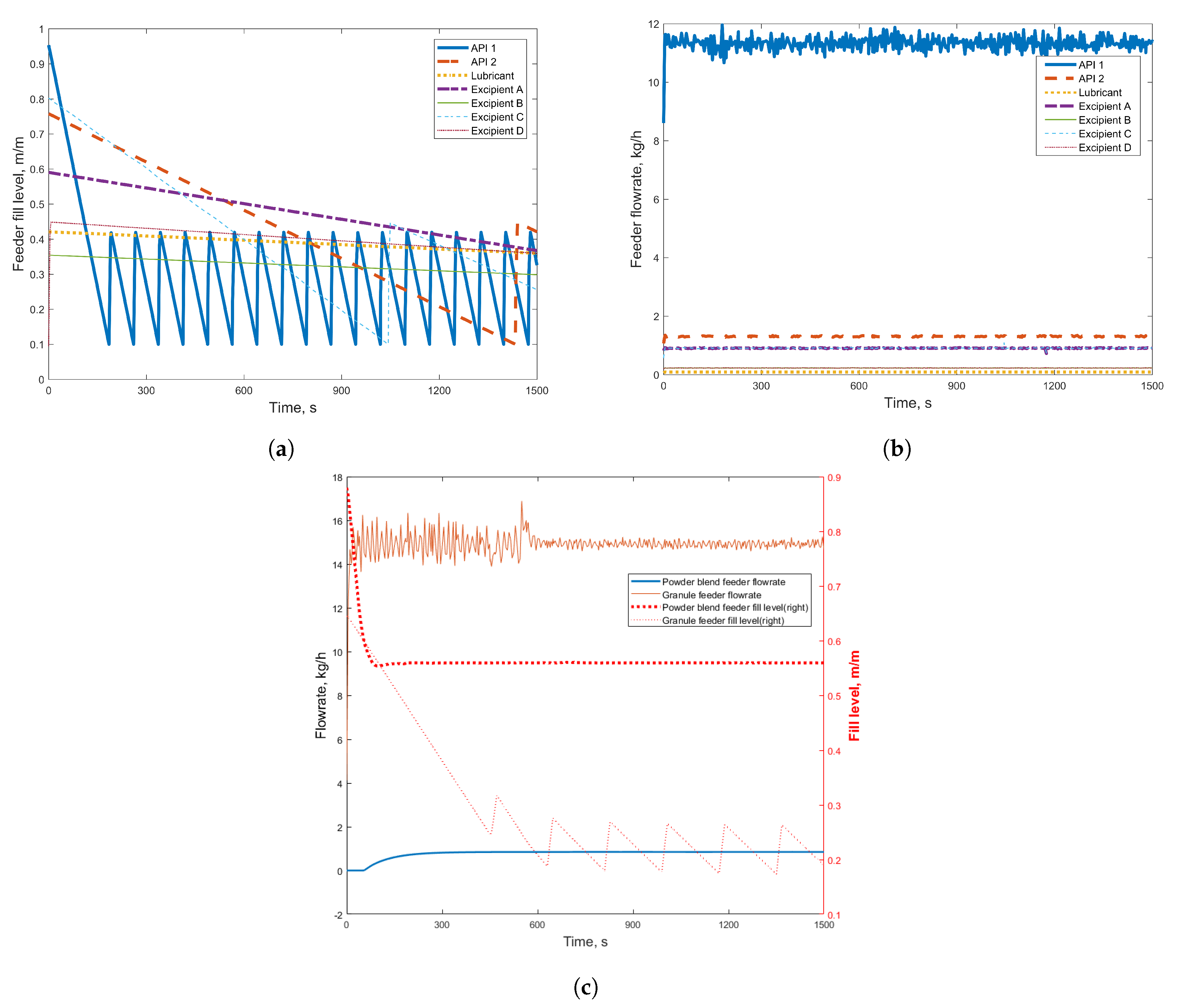
3.1. Simulation Results
3.2. Case Study
3.2.1. Case Study 1: Step Change in Feeder Flow Rate
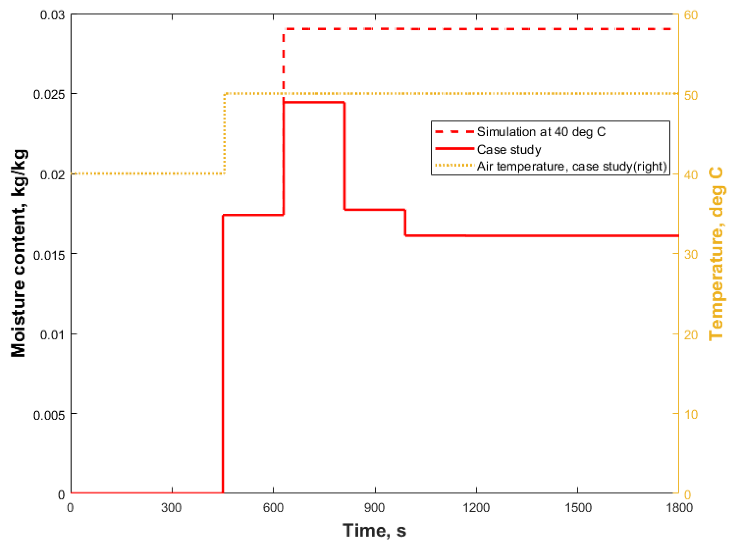
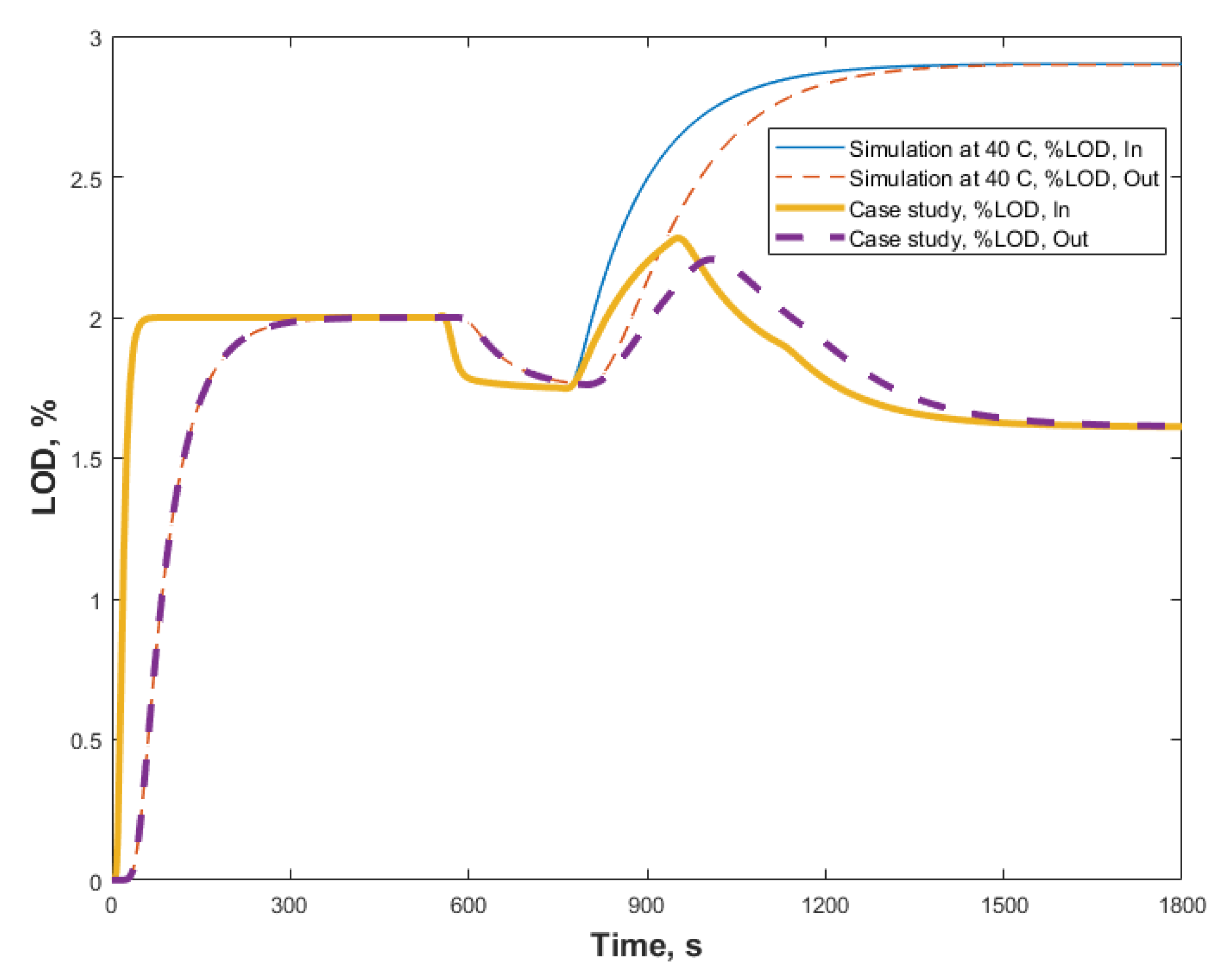
3.2.2. Case Study 2: Step Change in Dryer Air Temperature
3.3. Scenario Analysis Results
3.4. Sensitivity Analysis Results
4. Conclusions and Future Direction
Author Contributions
Funding
Acknowledgments
Conflicts of Interest
Acronyms
| PBM | population balance model |
| GSD | granule size distribution |
| PSD | particle size distribution |
| TSWG | twin-screw wet granulator |
| FBD | fluid bed dryer |
| CPPs | critical process parameters |
| CQAs | critical quality attributes |
| API | active pharmaceutical ingredients |
| CSTR | continuously stirred tank reactor |
| RTD | residence time distribution |
| MWC | mean weight control |
| LIW | Loss-in-weight |
| PLS | partial least squares |
| QbD | Quality-by-Design |
| PSE | Process Systems Engineering |
Nomenclature
| Unit | Symbol | Description |
| General | t | time |
| Feeder | Feed factor | |
| , , | Model parameters | |
| Screw speed | ||
| Mass flow rate, out | ||
| Blender | Time constant | |
| M | Mass holdup | |
| Steady state mass holdup | ||
| Mass flow rate, in | ||
| Mass flow rate, out | ||
| Axial dispersion time constant | ||
| API concentration, in | ||
| API concentration, out | ||
| Peclet number | ||
| Number of tanks | ||
| Granulator | n | Number density |
| x, | Particle volumes | |
| Collision frequency | ||
| Aggregation efficiency | ||
| b | Breakage fragment distribution | |
| , , , , , , | Aggregation kernel parameters | |
| S | Breakage selection rate | |
| Breakage rate constant | ||
| Standard deviation of a Gaussian distribution | ||
| Mean of a Gaussian distribution | ||
| volume fraction of erosion in breakage | ||
| Dryer | Mass transfer rate | |
| Mass transfer coefficient | ||
| Partial vapor density over the droplet surface | ||
| Partial vapor density in the ambient air | ||
| Droplet surface area | ||
| Specific heat of evaporation | ||
| Specific heat capacity liquid | ||
| Droplet mass | ||
| Uniform droplet temperature | ||
| h | Heat transfer coefficient | |
| Drying gas temperature | ||
| Droplet radius | ||
| Wet radius | ||
| Particle radius | ||
| Granule porosity | ||
| empirical coefficient | ||
| Vapor diffusion coefficient | ||
| Molecular weight liquid | ||
| Pressure of the drying air | ||
| ℜ | Ideal gas constant | |
| Temperature of solids at the granule surface | ||
| Temperature at particle gas-liquid interface | ||
| Partial vapor pressure drying air | ||
| Partial vapor pressure at gas-liquid interface | ||
| Temperature of the particle solids | ||
| X | Moisture content | |
| Equilibrium moisture content | ||
| Change in moisture content over time | ||
| Filling time | ||
| Drying time | ||
| f | Size fraction | |
| Average moisture content size fraction | ||
| Time | ||
| Dryer batch model parameter | ||
| API concentration | ||
| TSWG mass flow rate | ||
| Mill | M | Mass holdup |
| w,u | Particle volumes | |
| Rate of formation | ||
| Rate of depletion | ||
| Mass flow rate, in | ||
| Mass flow rate, out | ||
| K | Breakage kernel | |
| b | Breakage distribution function | |
| Impeller speed | ||
| Minimum impeller speed | ||
| Feed particle size distribution | ||
| Screen size | ||
| Critical screen size | ||
| p, q, , , , , | Model parameters | |
| Bulk density | ||
| Tablet Press | Delay time CSTR | |
| Delay time plug flow | ||
| Tablet cup volume | ||
| Tablet cup die surface | ||
| Tablet punch cup depth | ||
| True density | ||
| Bulk density | ||
| Tapped density | ||
| Fill density factor | ||
| Fill depth | ||
| Mean tablet weight | ||
| Volume of solids in tablet die | ||
| Main compression height | ||
| W | Tablet width | |
| T | Tablet thickness | |
| Upper punch penetration depth | ||
| P | Tablet potency | |
| Tablet volume | ||
| Relative density | ||
| N | Hardness | |
| Tensile strength | ||
| Critical density | ||
| Maximum tensile strength | ||
| PSD size span | ||
| Intermediate units | S | Signal to axial disperion model |
| z | Axial dispersion domain | |
| L | Transfer line length | |
| Plug flow time delay | ||
| Sensitivity analysis, Morris | Elementary effect for factor i | |
| Y | Model output | |
| Step change in input factor | ||
| Average elementary effect for factor i | ||
| Average absolute elementary effect for factor i | ||
| Variance of elementary effects for factor i | ||
| Sensitivity analysis, Variance based | Variance of matrix X | |
| Expectede values for matrix X | ||
| Sensitivity index for factor i | ||
| Total sensitivity index for factor i |
Appendix A
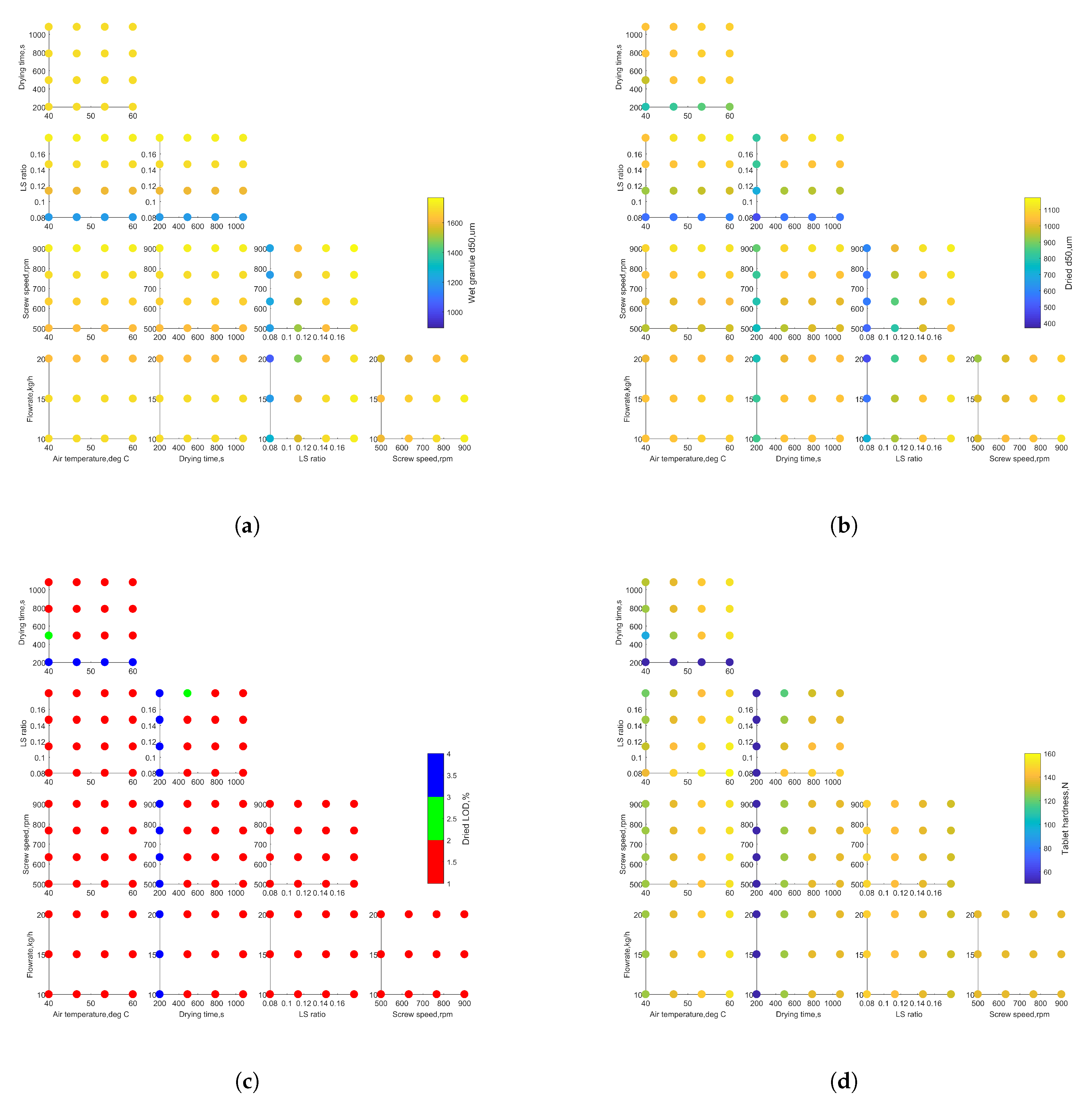
Appendix A.1. Morris Method Sensitivity Analysis
| Output → | d10, m | d50, m | d90, m | Moisture, kg/kg | ||||||||
| Input ↓ | ||||||||||||
| Air temperature | 0.11 | 0.21 | 0.30 | 0.52 | 0.87 | 1.29 | 0.98 | 1.77 | 2.59 | 0.00 | 0.00 | 0.00 |
| Drying time | 0.10 | 0.22 | 0.37 | 0.34 | 0.80 | 1.26 | 0.64 | 1.51 | 2.39 | 0.00 | 0.00 | 0.00 |
| LS ratio | 407.42 | 407.42 | 103.79 | 458.99 | 458.99 | 246.00 | 656.49 | 656.49 | 296.79 | 0.08 | 0.08 | 0.02 |
| Screw speed | 37.45 | 37.45 | 14.53 | 127.43 | 127.43 | 70.74 | 115.23 | 121.95 | 111.01 | 0.00 | 0.00 | 0.00 |
| Flow rate | −35.49 | 38.10 | 28.06 | −145.43 | 148.57 | 138.75 | −148.87 | 154.33 | 136.70 | 0.00 | 0.00 | 0.00 |
| Output → | d10, m | d50, m | d90, m | Moisture, % | ||||||||
| Input ↓ | ||||||||||||
| Air temperature | 17.30 | 17.39 | 17.79 | 81.69 | 82.11 | 55.76 | 139.08 | 139.79 | 103.01 | −2.01 | 2.01 | 1.64 |
| Drying time | 22.77 | 22.94 | 36.96 | 101.87 | 102.56 | 139.46 | 182.81 | 184.14 | 243.99 | −2.77 | 2.77 | 3.50 |
| LS ratio | 273.71 | 273.71 | 81.03 | 410.60 | 410.60 | 206.75 | 307.38 | 326.94 | 200.84 | 1.50 | 1.50 | 1.93 |
| Screw speed | 18.03 | 18.03 | 7.37 | 121.74 | 121.74 | 53.72 | 86.86 | 86.86 | 48.09 | 0.00 | 0.00 | 0.00 |
| Flow rate | −22.44 | 22.44 | 11.43 | −109.86 | 115.99 | 99.38 | −102.19 | 114.15 | 96.78 | 0.00 | 0.00 | 0.00 |
| Output → | Bulk Density, Kg/m | Tapped Density, Kg/m | Angle of Repose, deg | ||||||
| Input ↓ | |||||||||
| Air temperature | −6.19 | 6.24 | 5.89 | −4.75 | 4.78 | 4.53 | 0.79 | 0.80 | 0.62 |
| Drying time | -8.30 | 8.33 | 12.12 | −6.21 | 6.23 | 8.76 | 1.07 | 1.08 | 1.50 |
| LS ratio | 16.70 | 16.70 | 11.80 | 11.25 | 11.39 | 8.56 | 1.17 | 1.43 | 1.20 |
| Screw speed | −14.25 | 14.25 | 5.73 | −12.32 | 12.32 | 4.64 | 0.85 | 0.85 | 0.40 |
| Flow rate | 4.53 | 6.99 | 7.71 | 3.82 | 5.23 | 5.57 | −0.63 | 0.80 | 0.76 |
| Output → | d10, m | d50, m | d90, m | Span | ||||||||
| Input ↓ | ||||||||||||
| Air temperature | 4.81 | 4.81 | 5.06 | 7.94 | 7.96 | 5.06 | 8.76 | 8.80 | 6.68 | −0.02 | 0.02 | 0.01 |
| Drying time | 6.50 | 6.56 | 10.44 | 9.45 | 9.52 | 12.07 | 11.21 | 11.27 | 13.85 | −0.02 | 0.02 | 0.03 |
| LS ratio | 146.63 | 146.63 | 46.95 | 252.14 | 252.14 | 68.84 | 83.55 | 83.55 | 31.47 | −0.96 | 0.96 | 0.29 |
| Screw speed | 3.38 | 3.68 | 3.56 | 3.16 | 9.13 | 10.91 | 16.16 | 16.53 | 10.26 | 0.01 | 0.03 | 0.03 |
| Flow rate | −7.63 | 8.39 | 8.91 | −8.83 | 13.65 | 12.13 | −16.54 | 19.73 | 23.27 | 0.01 | 0.05 | 0.06 |
| Output → | Bulk Density, Kg/m | Tapped Density, Kg/m | ||||
| Input ↓ | ||||||
| Air temperature | 4.93 | 4.93 | 3.24 | 4.09 | 4.09 | 2.54 |
| Drying time | 5.34 | 5.39 | 6.93 | 4.33 | 4.38 | 5.59 |
| LS ratio | 237.08 | 237.08 | 62.79 | 236.53 | 236.53 | 57.64 |
| Screw speed | 1.76 | 5.14 | 8.27 | −16.09 | 17.69 | 14.84 |
| Flow rate | −13.81 | 13.81 | 5.26 | −8.02 | 12.52 | 14.14 |
| Output → | Hardness, N | Potency, g | Compression Height, mm | Fill Depth, mm | ||||||||
| Input ↓ | ||||||||||||
| Air temperature | 28.85 | 28.85 | 38.87 | 0.00 | 0.00 | 0.00 | 0.37 | 0.37 | 1.67 | 0.85 | 0.96 | 4.05 |
| Drying time | 84.89 | 84.89 | 100.13 | 0.00 | 0.00 | 0.00 | 2.62 | 2.62 | 3.71 | 4.57 | 4.63 | 6.83 |
| LS ratio | −21.40 | 21.40 | 38.55 | 0.00 | 0.00 | 0.00 | −0.37 | 0.37 | 1.67 | −3.83 | 3.83 | 4.10 |
| Screw speed | 0.01 | 0.27 | 0.41 | 0.00 | 0.00 | 0.00 | 0.00 | 0.00 | 0.00 | −0.02 | 0.14 | 0.24 |
| Flow rate | 0.06 | 0.49 | 0.66 | 0.00 | 0.00 | 0.00 | 0.00 | 0.00 | 0.00 | 0.22 | 0.22 | 0.21 |
| Output → | Time Constant, s | Number of Tanks | Steady State Holdup, kg | ||||||
| Input ↓ | |||||||||
| Air temperature | 0.00 | 0.00 | 0.00 | 0.00 | 0.00 | 0.00 | 0.00 | 0.00 | 0.00 |
| Drying time | 0.00 | 0.00 | 0.00 | 0.00 | 0.00 | 0.00 | 0.00 | 0.00 | 0.00 |
| LS ratio | −0.00 | 0.00 | 0.00 | 0.00 | 0.00 | 0.00 | 0.00 | 0.00 | 0.00 |
| Screw speed | 0.00 | 0.00 | 0.00 | 0.00 | 0.00 | 0.00 | 0.00 | 0.00 | 0.00 |
| Flow rate | −15.53 | 15.53 | 3.68 | −0.15 | 0.15 | 0.07 | 0.03 | 0.03 | 0.01 |
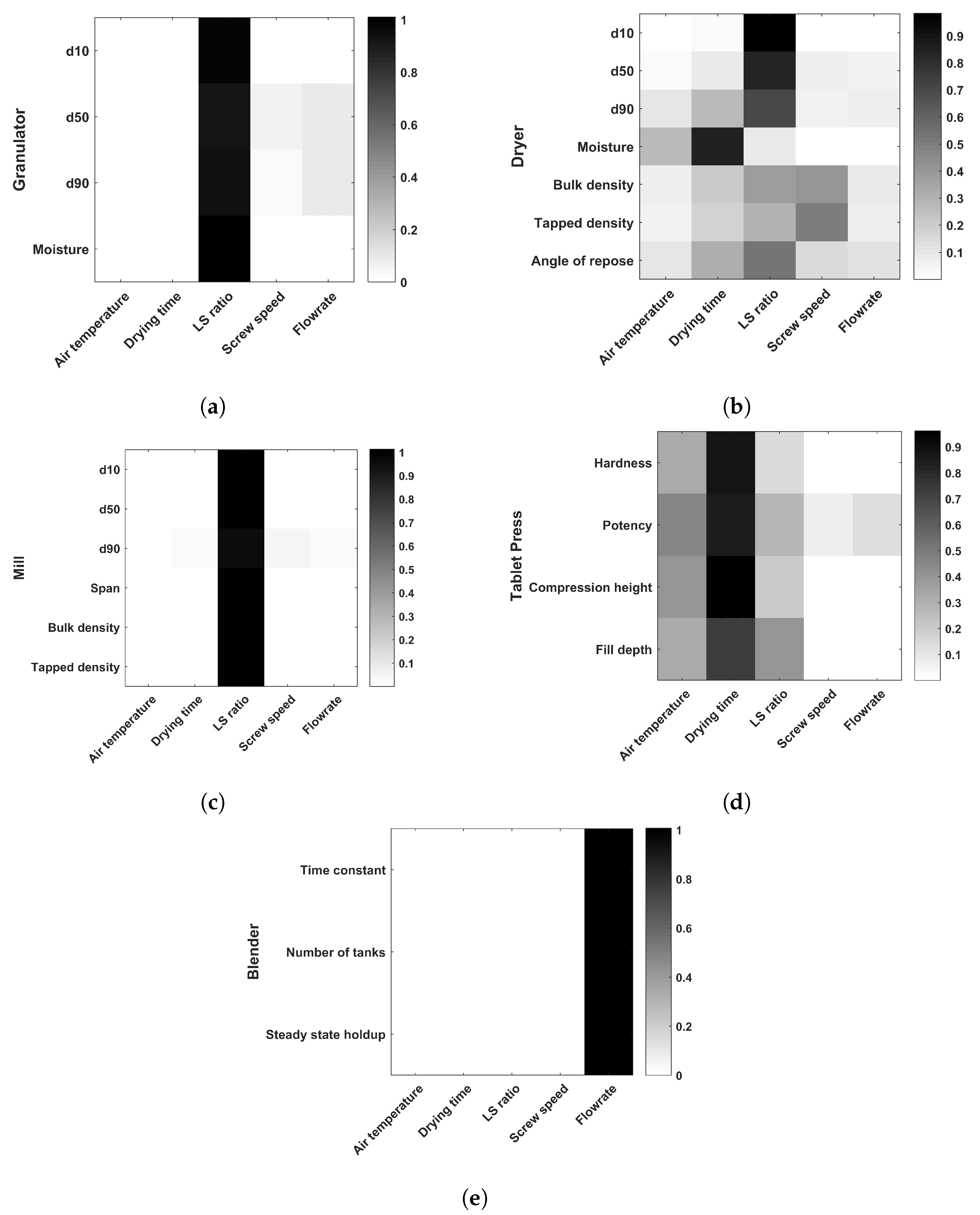
Appendix A.2. Variance Based Sensitivity Analysis
| Output → | d10 | d50 | d90 | Moisture | ||||
| Input ↓ | ||||||||
| Air temperature | 0.00 | 0.00 | 0.00 | 0.00 | 0.00 | 0.00 | 0.00 | 0.00 |
| Drying time | 0.00 | 0.00 | 0.00 | 0.00 | 0.00 | 0.00 | 0.00 | 0.00 |
| LS ratio | 0.98 | 0.99 | 0.87 | 0.92 | 0.90 | 0.94 | 1.00 | 1.01 |
| Screw speed | 0.00 | 0.01 | 0.03 | 0.05 | 0.00 | 0.02 | 0.00 | 0.00 |
| Flow rate | 0.00 | 0.01 | 0.03 | 0.09 | 0.03 | 0.09 | 0.00 | 0.00 |
| Output → | d10 | d50 | d90 | Moisture | ||||
| Input ↓ | ||||||||
| Air temperature | 0.00 | 0.01 | 0.00 | 0.03 | 0.04 | 0.10 | 0.11 | 0.27 |
| Drying time | 0.01 | 0.02 | 0.05 | 0.08 | 0.17 | 0.27 | 0.64 | 0.85 |
| LS ratio | 0.97 | 0.98 | 0.78 | 0.84 | 0.58 | 0.70 | 0.00 | 0.08 |
| Screw speed | 0.00 | 0.01 | 0.04 | 0.07 | 0.01 | 0.05 | 0.00 | 0.00 |
| Flow rate | 0.00 | 0.01 | 0.01 | 0.06 | 0.00 | 0.06 | 0.00 | 0.00 |
| Output → | Bulk Density | Tapped Density | Angle of Repose | |||
| Input ↓ | ||||||
| Air temperature | 0.01 | 0.06 | 0.01 | 0.06 | 0.04 | 0.11 |
| Drying time | 0.12 | 0.20 | 0.11 | 0.18 | 0.21 | 0.32 |
| LS ratio | 0.24 | 0.38 | 0.19 | 0.30 | 0.38 | 0.53 |
| Screw speed | 0.40 | 0.41 | 0.49 | 0.50 | 0.11 | 0.15 |
| Flow rate | 0.00 | 0.08 | 0.00 | 0.07 | 0.00 | 0.11 |
| Output → | d10 | d50 | d90 | Span | ||||
| Input ↓ | ||||||||
| Air temperature | 0.00 | 0.00 | 0.00 | 0.00 | 0.00 | 0.01 | 0.00 | 0.00 |
| Drying time | 0.00 | 0.00 | 0.00 | 0.00 | 0.00 | 0.02 | 0.00 | 0.00 |
| LS ratio | 0.99 | 1.00 | 0.99 | 1.01 | 0.91 | 0.96 | 0.99 | 1.01 |
| Screw speed | 0.00 | 0.00 | 0.00 | 0.00 | 0.02 | 0.04 | 0.00 | 0.00 |
| Flow rate | 0.00 | 0.01 | 0.00 | 0.00 | 0.00 | 0.03 | 0.00 | 0.00 |
| Output → | Bulk Density | Tapped Density | ||
| Input ↓ | ||||
| Air temperature | 0.00 | 0.00 | 0.00 | 0.00 |
| Drying time | 0.00 | 0.00 | 0.00 | 0.00 |
| LS ratio | 1.00 | 1.01 | 0.99 | 1.00 |
| Screw speed | 0.00 | 0.00 | 0.00 | 0.01 |
| Flow rate | 0.00 | 0.00 | 0.00 | 0.00 |
| Output → | Hardness | Potency | Compression Height | Fill Depth | ||||
| Input ↓ | ||||||||
| Air temperature | 0.14 | 0.33 | 0.04 | 0.45 | 0.08 | 0.39 | 0.08 | 0.32 |
| Drying time | 0.58 | 0.88 | 0.52 | 0.85 | 0.51 | 0.96 | 0.40 | 0.72 |
| LS ratio | 0.03 | 0.14 | 0.01 | 0.28 | 0.02 | 0.21 | 0.26 | 0.40 |
| Screw speed | 0.00 | 0.00 | 0.00 | 0.07 | 0.00 | 0.00 | 0.00 | 0.00 |
| Flow rate | 0.00 | 0.00 | 0.02 | 0.13 | 0.00 | 0.00 | 0.00 | 0.00 |
| Output → | Time Constant | Number of Tanks | Steady State Holdup | |||
| Input ↓ | ||||||
| Air temperature | 0.00 | 0.00 | 0.00 | 0.00 | 0.00 | 0.00 |
| Drying time | 0.00 | 0.00 | 0.00 | 0.00 | 0.00 | 0.00 |
| LS ratio | 0.00 | 0.00 | 0.00 | 0.00 | 0.00 | 0.00 |
| Screw speed | 0.00 | 0.00 | 0.00 | 0.00 | 0.00 | 0.00 |
| Flow rate | 1.00 | 1.00 | 1.00 | 1.01 | 1.00 | 1.00 |
References
- Escotet-Espinoza, M.S.; Singh, R.; Sen, M.; O’Connor, T.; Lee, S.; Chatterjee, S.; Ramachandran, R.; Ierapetritou, M.G.; Muzzio, F.J. Flowsheet Models Modernize Pharmaceutical Manufacturing Design and Risk Assessment. Pharm. Technol. 2015, 39, 34–42. [Google Scholar]
- Gernaey, K.V.; Cervera-Padrell, A.E.; Woodley, J.M. A perspective on PSE in pharmaceutical process development and innovation. Comput. Chem. Eng. 2012, 42, 15–29. [Google Scholar] [CrossRef]
- Wang, Z.; Escotet-Espinoza, M.S.; Ierapetritou, M. Process analysis and optimization of continuous pharmaceutical manufacturing using flowsheet models. Comput. Chem. Eng. 2017, 107, 77–91. [Google Scholar] [CrossRef]
- Galbraith, S.C.; Huang, Z.; Cha, B.; Liu, H.; Hurley, S.; Flamm, M.H.; Meyer, R.J.; Yoon, S. Flowsheet Modeling of a Continuous Direct Compression Tableting Process at Production Scale. In Proceedings of the Foundations of Computer Aided Process Operations/Chemical Process Control, Tucson, AZ, USA, 8–12 January 2017. [Google Scholar]
- Rogers, A.J.; Inamdar, C.; Ierapetritou, M.G. An Integrated Approach to Simulation of Pharmaceutical Processes for Solid Drug Manufacture. Ind. Eng. Chem. Res. 2014, 53, 5128–5147. [Google Scholar] [CrossRef]
- García-Muñoz, S.; Butterbaugh, A.; Leavesley, I.; Manley, L.F.; Slade, D.; Bermingham, S. A flowsheet model for the development of a continuous process for pharmaceutical tablets: An industrial perspective. AIChE J. 2018, 64, 511–525. [Google Scholar] [CrossRef]
- Park, S.Y.; Galbraith, S.C.; Liu, H.; Lee, H.; Cha, B.; Huang, Z.; O’Connor, T.; Lee, S.; Yoon, S. Prediction of critical quality attributes and optimization of continuous dry granulation process via flowsheet modeling and experimental validation. Powder Technol. 2018, 330, 461–470. [Google Scholar] [CrossRef]
- Boukouvala, F.; Niotis, V.; Ramachandran, R.; Muzzio, F.J.; Ierapetritou, M.G. An integrated approach for dynamic flowsheet modeling and sensitivity analysis of a continuous tablet manufacturing process. Comput. Chem. Eng. 2012, 42, 30–47. [Google Scholar] [CrossRef]
- Boukouvala, F.; Chaudhury, A.; Sen, M.; Zhou, R.; Mioduszewski, L.; Ierapetritou, M.G.; Ramachandran, R. Computer-Aided Flowsheet Simulation of a Pharmaceutical Tablet Manufacturing Process Incorporating Wet Granulation. J. Pharm. Innov. 2013, 8, 11–27. [Google Scholar] [CrossRef]
- Boukouvala, F.; Ierapetritou, M.G. Surrogate-based optimization of expensive flowsheet modeling for continuous pharmaceutical manufacturing. J. Pharm. Innov. 2013, 8, 131–145. [Google Scholar] [CrossRef]
- Rogers, A.; Ierapetritou, M. Challenges and opportunities in modeling pharmaceutical manufacturing processes. Comput. Chem. Eng. 2015, 81, 32–39. [Google Scholar] [CrossRef]
- Verstraeten, M.; Van Hauwermeiren, D.; Lee, K.; Turnbull, N.; Wilsdon, D.; am Ende, M.; Doshi, P.; Vervaet, C.; Brouckaert, D.; Mortier, S.T.; et al. In-depth experimental analysis of pharmaceutical twin-screw wet granulation in view of detailed process understanding. Int. J. Pharm. 2017, 529, 678–693. [Google Scholar] [CrossRef] [PubMed]
- Van Hauwermeiren, D.; Verstraeten, M.; Doshi, P.; am Ende, M.T.; Turnbull, N.; Lee, K.; De Beer, T.; Nopens, I. On the modelling of granule size distributions in twin-screw wet granulation: Calibration of a novel compartmental population balance model. Powder Technol. 2018, 341, 116–125. [Google Scholar] [CrossRef]
- De Leersnyder, F.; Vanhoorne, V.; Bekaert, H.; Vercruysse, J.; Ghijs, M.; Bostijn, N.; Verstraeten, M.; Cappuyns, P.; Van Assche, I.; Vander Heyden, Y.; et al. Breakage and drying behaviour of granules in a continuous fluid bed dryer: Influence of process parameters and wet granule transfer. Eur. J. Pharm. Sci. 2018, 115, 223–232. [Google Scholar] [CrossRef] [PubMed]
- Ghijs, M.; Schäfer, E.; Kumar, A.; Cappuyns, P.; Van Assche, I.; De Leersnyder, F.; Vanhoorne, V.; De Beer, T.; Nopens, I. Modeling of Semicontinuous Fluid Bed Drying of Pharmaceutical Granules With Respect to Granule Size. J. Pharm. Sci. 2019. [Google Scholar] [CrossRef] [PubMed]
- Metta, N.; Verstraeten, M.; Ghijs, M.; Kumar, A.; Schafer, E.; Singh, R.; De Beer, T.; Nopens, I.; Cappuyns, P.; Van Assche, I.; Ierapetritou, M.; Ramachandran, R. Model development and prediction of particle size distribution, density and friability of a comilling operation in a continuous pharmaceutical manufacturing process. Int. J. Pharm. 2018, 549, 271–282. [Google Scholar] [CrossRef] [PubMed]
- Pantelides, C.C.; Nauta, M.; Matzopoulos, M.; Grove, H. Equation-Oriented Process Modelling Technology: Recent Advances & Current Perspectives. In Proceedings of the 5th Annual TRC-Idemitsu Work, Abu Dhabi, UAE, 15 February 2015. [Google Scholar]
- Escotet Espinoza, M. Phenomenological and Residence Time Distribution Models for Unit Operations in a Continuous Pharmaceutical Manufacturing Process. Ph.D. Thesis, Rutgers, The State University of New Jersey, Brunswick, NJ, USA, 2018. [Google Scholar]
- Abuaf, N.; Staub, F.W. Drying of Liquid–Solid Slurry Droplets. In Drying ’86; Mujumdar, A.S., Ed.; Hemisphere: Washington, DC, USA, 1986; Volume 1, pp. 227–248. [Google Scholar]
- Pitt, K.G.; Newton, J.M.; Richardson, R.; Stanley, P. The Material Tensile Strength of Convex-faced Aspirin Tablets. J. Pharm. Pharmacol. 1989, 41, 289–292. [Google Scholar] [CrossRef] [PubMed]
- Kuentz, M.; Leuenberger, H. A new model for the hardness of a compacted particle system, applied to tablets of pharmaceutical polymers. Powder Technol. 2000, 111, 145–153. [Google Scholar] [CrossRef]
- Engisch, W.; Muzzio, F. Using Residence Time Distributions (RTDs) to Address the Traceability of Raw Materials in Continuous Pharmaceutical Manufacturing. J. Pharm. Innov. 2016, 11, 64–81. [Google Scholar] [CrossRef] [PubMed]
- Saltelli, A.; Ratto, M.; Andres, T.; Campolongo, F.; Cariboni, J.; Gatelli, D.; Saisana, M.; Tarantola, S. Global Sensitivity Analysis: The Primer; Wiley: Hoboken, NJ, USA, 2008. [Google Scholar]
- Cryer, S.A.; Scherer, P.N. Observations and process parameter sensitivities in fluid-bed granulation. AIChE J. 2003, 49, 2802–2809. [Google Scholar] [CrossRef]
- Iooss, B.; Lemaître, P. A Review on Global Sensitivity Analysis Methods. In Uncertainty Management in Simulation-Optimization of Complex Systems: Algorithms and Applications; Dellino, G., Meloni, C., Eds.; Springer: New York, NY, USA, 2015; pp. 101–122. [Google Scholar] [CrossRef]
- Helton, J.C.; Davis, F.J. Latin hypercube sampling and the propagation of uncertainty in analyses of complex systems. Reliab. Eng. Syst. Saf. 2003, 81, 23–69. [Google Scholar] [CrossRef]


| Component Name | Weight % |
|---|---|
| API 1 | 75.58 |
| API 2 | 8.72 |
| Lubricant | 0.58 |
| Excipient A | 6.05 |
| Excipient B | 1.51 |
| Excipient C | 6.05 |
| Excipient D | 1.51 |
| Process Setting | Lower Bound | Upper Bound |
|---|---|---|
| Mass flow rate (kg/h) | 10 | 20 |
| Screw speed (RPM) | 500 | 900 |
| Liquid/solid-ratio (kg/kg ) | 0.08 | 0.18 |
| Unit | Initial State | Dynamic State |
|---|---|---|
| Feeders | Full | Refills when empty |
| Blender | Empty | Reaches steady state |
| Granulator | Empty | Output obtained when input is in studied range |
| Plug flow delay added to instantaneous response | ||
| Dryer | Empty | Releases batches of material at the end of drying time |
| Mill | Empty | Releases material in semi-continuous mode |
| Tablet Press | Empty | Output obtained when input is in studied range |
| Delay from RTD model in feed frame | ||
| Powder blend feeder | Full with powder blend | Continuous feed from blender |
| Granule feeder | Full with granules | Refill from mill |
| Granule blender | Always full | Delay from axial dispersion |
| Unit | Factor | Bounds | Number of Levels | Response |
|---|---|---|---|---|
| Blender | flowrate setpoint, kg/h | [10, 20] | 3 | Mean Residence time |
| Number of tanks | ||||
| Granulator | LS ratio, kg/kg | [0.08, 0.18] | 4 | PSD: d10, d50, d90 |
| Screw speed, rpm | [500, 900] | 4 | Moisture content | |
| Dryer | Air temperature, deg C | [40, 60] | 4 | PSD: d10, d50, d90 |
| Drying time, s | [200, 1080] | 4 | Moisture content | |
| Mill | PSD: d10, d50, d90 | |||
| Span | ||||
| Bulk density | ||||
| Tapped density | ||||
| Tablet Press | Tablet hardness | |||
| Tablet potency | ||||
| MCH | ||||
| Fill depth |
| Unit | Process Variable | Units | Value |
|---|---|---|---|
| Feeders | API 1 flow rate | kg/h | 11.337 |
| API 2 flow rate | kg/h | 1.308 | |
| Lubricant flow rate | kg/h | 0.087 | |
| Excipient A flow rate | kg/h | 0.907 | |
| Excipient B flow rate | kg/h | 0.227 | |
| Excipient C flow rate | kg/h | 0.907 | |
| Excipient D flow rate | kg/h | 0.227 | |
| Powder blend feeder flow rate | kg/h | 14.913 | |
| Granule feeder flow rate | kg/h | 14.913 | |
| Blenders | Bladespeed | rpm | 250 |
| Granulator | Liquid-solid ratio | kg/kg | 0.12 |
| Screw speed | rpm | 500 | |
| Dryer | Air flow | m/h | 360 |
| Air temperature | deg C | 40 | |
| Drying time | s | 450 | |
| Filling time | s | 180 | |
| Tablet Press | Turret speed | rpm | 29.8 |
| Mean weight | g | 0.43 |
© 2019 by the authors. Licensee MDPI, Basel, Switzerland. This article is an open access article distributed under the terms and conditions of the Creative Commons Attribution (CC BY) license (http://creativecommons.org/licenses/by/4.0/).
Share and Cite
Metta, N.; Ghijs, M.; Schäfer, E.; Kumar, A.; Cappuyns, P.; Van Assche, I.; Singh, R.; Ramachandran, R.; De Beer, T.; Ierapetritou, M.; et al. Dynamic Flowsheet Model Development and Sensitivity Analysis of a Continuous Pharmaceutical Tablet Manufacturing Process Using the Wet Granulation Route. Processes 2019, 7, 234. https://0-doi-org.brum.beds.ac.uk/10.3390/pr7040234
Metta N, Ghijs M, Schäfer E, Kumar A, Cappuyns P, Van Assche I, Singh R, Ramachandran R, De Beer T, Ierapetritou M, et al. Dynamic Flowsheet Model Development and Sensitivity Analysis of a Continuous Pharmaceutical Tablet Manufacturing Process Using the Wet Granulation Route. Processes. 2019; 7(4):234. https://0-doi-org.brum.beds.ac.uk/10.3390/pr7040234
Chicago/Turabian StyleMetta, Nirupaplava, Michael Ghijs, Elisabeth Schäfer, Ashish Kumar, Philippe Cappuyns, Ivo Van Assche, Ravendra Singh, Rohit Ramachandran, Thomas De Beer, Marianthi Ierapetritou, and et al. 2019. "Dynamic Flowsheet Model Development and Sensitivity Analysis of a Continuous Pharmaceutical Tablet Manufacturing Process Using the Wet Granulation Route" Processes 7, no. 4: 234. https://0-doi-org.brum.beds.ac.uk/10.3390/pr7040234