Predicting the Longitudinally and Radially Varying Gut Microbiota Composition using Multi-Scale Microbial Metabolic Modeling

Abstract

Background: The gut microbiota is a heterogeneous group of microbes that is spatially distributed along various sections of the intestines and across the mucosa and lumen in each section. Understanding the dynamics between the spatially differential microbial populations and the driving forces for the observed spatial organization will provide valuable insights into important questions such as the nature of colonization of the infant gut and different types of inflammatory bowel disease localized in different regions of the intestines. However, in most studies, the microbiota is sampled only at a single site (often feces) or from a particular anatomical site of the intestines. Differential oxygen availability is putatively a key factor shaping the spatial organization. Results: To test this hypothesis, we constructed a community genome-scale metabolic model consisting of representative organisms for the major phyla present in the human gut microbiome. By solving step-wise optimization problems embedded in a dynamic framework to predict community metabolism and integrate the mucosally-adherent with the luminal microbiome between consecutive sections along the intestines, we were able to capture (i) the essential features of the spatially differential composition of obligate anaerobes vs. facultative anaerobes and aerobes determined experimentally, and (ii) the accumulation of microbial biomass in the lumen. Sensitivity analysis suggests that the spatial organization depends primarily on the oxygen-per-microbe availability in each region. Oxygen availability is reduced relative to the ~100-fold increase in mucosal microbial density along the intestines, causing the switch between aerobes and anaerobes. Conclusion: The proposed integrated dynamic framework is able to predict spatially differential gut microbiota composition using microbial genome-scale metabolic models and test hypotheses regarding the dynamics of the gut microbiota. It can potentially become a valuable tool for exploring therapeutic strategies for site-specific perturbation of the gut microbiota and the associated metabolic activities.

1. Background

The human gut microbiota has been shown to be extremely influential in human health. It participates in various aspects of the human physiology, ranging from energy metabolism, immune response, bile acid metabolism, intestinal function and integrity, bone homeostasis to brain function and nerve system [1]. The gut microbiota has been implicated in the onset of a number of diseases. These include the inflammatory bowel disease (IBD), obesity, non-alcoholic fatty liver, type 2 diabetes and colorectal cancer [2]. Unraveling the interactions between gut microbes and drug metabolism (e.g., [3,4,5,6]) is becoming a significant factor in evaluating drug efficacy and toxicity [7]. It is therefore important to identify the factors that shape the composition of the gut microbiome and its function. Out of these factors, diet, from which the primary nutrients for the gut microbiome originate, has been widely studied [8,9,10,11,12,13] and while very important, it is not the sole determinant factor [14]. Other factors, such as host genotype [15], age, geographical location [16], circadian cycle [17] and history of antibiotic treatments [18,19], have also been assessed. While a large amount of gut microbiome studies have relied on comparing only the fecal microbiome or the microbiome in a particular section of the intestines, multiple studies have shown that the microbiome varies not only longitudinally along the intestines, but also radially between the mucosal surface and the lumen in each section of the intestines [12,20,21,22,23,24]. The spatially differential microbiome is likely the result of the differences in the biochemical, as well as physical properties of different intestinal anatomical sites, such as nutrient and oxygen concentrations [22], pH, and mucus viscosity [25].

To systematically analyze the impact of these properties on the spatial organization of the gut microbiome, a computational model integrating both the dynamics of bacterial growth and the spatial characteristics of the intestines is needed. Genome-scale metabolic models can predict the growth and metabolism of bacteria given the nutrients available using flux balance analysis (FBA) [26,27] and can be integrated into dynamic frameworks to describe biomass production and changes in metabolite concentrations over time through dynamic flux balance analysis (dFBA) [28,29]. The approach has been extensively applied to microbial communities [30,31,32,33,34,35], in particular gut microbiota [36,37,38,39,40,41,42,43,44] and integrated with dynamic frameworks [45,46,47,48] and spatiotemporal elements [49,50,51,52,53] (reviewed in references [54,55,56]). In this study, we analyzed the impact of the differential oxygen availability on the mucosal adherent microbiota and the luminal microbiota and their compositions. They were modeled as two distinct communities that are able to exchange metabolites and microbial biomass in each section of the intestines (see Figure 1A). Consecutive sections are connected by the flow of the luminal contents including microbes. Using this framework, microbiota compositions with a surprising high level of agreement with experimentally captured distributions of obligate anaerobes and facultative anaerobes were predicted [22,23,24]. This alludes to the possibility of using computations to predict the effect of perturbations on the spatially distributed microbial composition in the intestines.

2. Results

2.1. A dynamic Framework for Simulating Spatially Differential Gut Microbiota Metabolism

A dynamic model was assembled for simulating the spatial distribution of gut microbes along the intestines. The intestine was divided into seven sections according to anatomical considerations: proximal, middle and distal small intestine; cecum, and; proximal, middle and distal large intestine. There are two distinct communities defined in each section of the intestines: the mucosal microbiota adherent to the mucus layer and the luminal microbiota residing in the intestinal lumen. Figure 1A shows five processes being modeled (marked by roman numerals) and Figure 1B describes the corresponding simulation procedure. In each section of the intestines, the simulation was performed for a period of time equal to the retention time of the luminal contents. The initial luminal contents in each section are equal to the luminal contents at the end of the simulation for the previous intestinal section (including the microbes in the lumen), or the nutrients from the diet for the first section (Step I). In addition to the nutrients available in the luminal contents, oxygen diffused from intestinal epithelial cells is available to the microbiota (Step II, see Oxygen availability in Materials and Methods). The luminal microbiota changes over time and its growth was modeled using a previous procedure [45] (Step III, see Luminal microbiota in Materials and Methods). During the simulation, the mucosal microbiota was assumed to be relatively stable along the time-course of the experiment and was modeled using the SteadyCom framework [43] (Step IV, see Mucosal microbiota in Materials and Methods). Shedding from the mucosal microbiota also contributed to the increase in the luminal microbial biomass (Step V, see Connecting the luminal and mucosal microbiota in Materials and Methods). In each section of the intestines, the microbial community metabolic network consisting of representative species of the gut microbiota is identical for both the mucosal and luminal microbiota (including obligate anaerobes, facultative anaerobes and aerobes; see Metabolic models and nutrients available in Materials and Methods). The described algorithms and dynamics however allow for the simulation of microbiota abundance profiles that are location-specific.

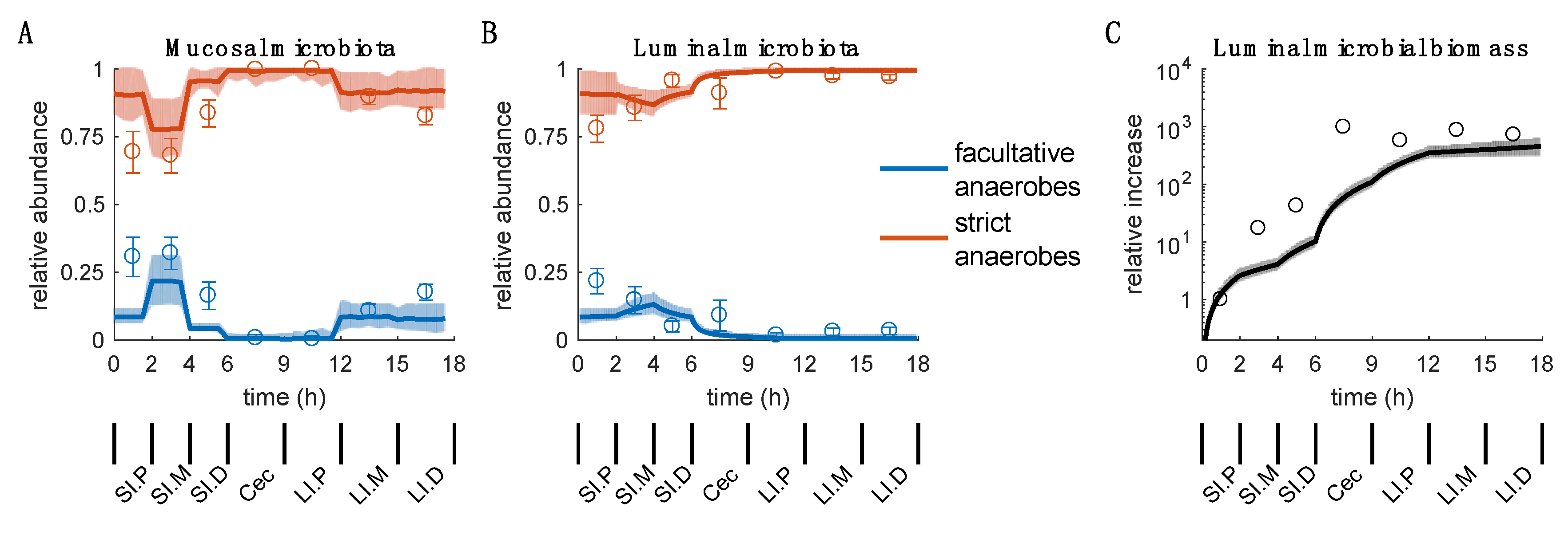
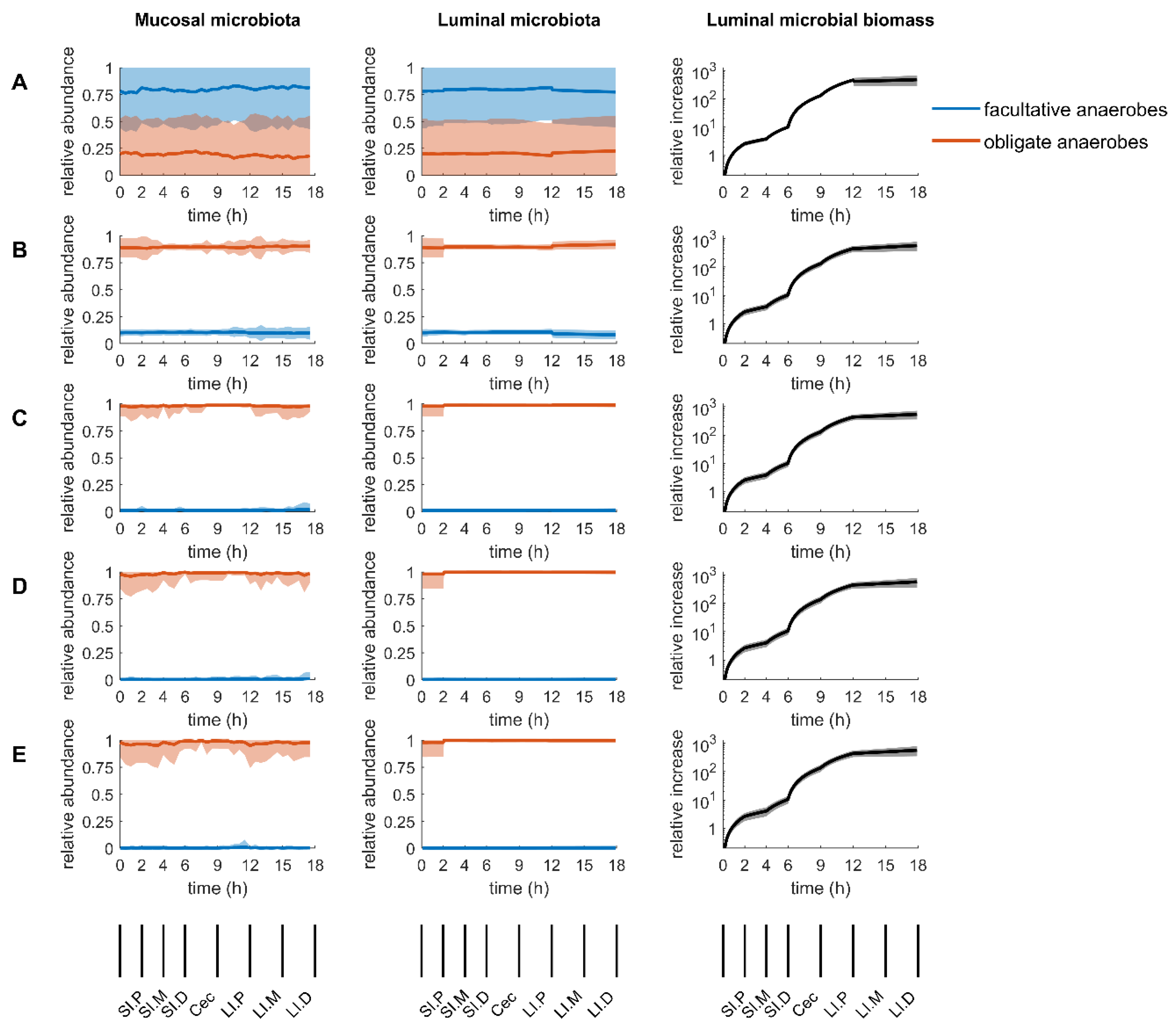
2.2. Overview of the Simulation Results

1000 simulations were performed using the default set of parameters from Table 2, Table 3 and Table 4 in which the total oxygen flux available was constant while the oxygen flux available to the luminal microbiota decreased as the luminal content progressed along the intestines (Figure 2). Interestingly, the simulation results (see Figure 2) showed changes in the composition of obligate anaerobes vs. aerobes and facultative anaerobes in both the mucosal and luminal microbiota that are strikingly similar to the experimental results in reference [24]. From sensitive analysis of the parameters in the model, the oxygen-per-mucosal-biomass availability $r_{oxygen}^{total} / X_{muc}^{total}$ that largely varies along the intestines, was found to be the most significant determinant of the spatial distribution. Perturbations in the oxygen-related parameters that are small compared to the experimentally observed variation in the mucosal biomass density had no qualitative impact on the distribution. These results are described in detail in the following subsections.

2.3. Mucosal Microbiota

For the mucosal microbiota, aerobes and facultative anaerobes (E. coli and C. glutamicum in the model) have relatively high abundance in the small intestine, close-to-zero abundance in cecum and proximal large intestine and a rebound in the middle and distal large intestines (Figure 2A). The simulation results recapitulated the trend and suggested that the primary factor shaping the abundances for aerobes and facultative anaerobes vs. obligate anaerobes in the mucosal microbiota was the large difference in biomass density in different sections of the intestines (100-fold increase in both the cecum and the proximal large intestine compared to other sections, Table 1). Because the total oxygen available to the community was kept constant, the oxygen available per gram of dry weight of microbes decreases with increasing total biomass density from the middle small intestine to the proximal large intestine. The abundance of aerobes or facultative anaerobes therefore consequently decreases. Because the magnitude difference in biomass density is large (100-fold), this trend was likely to hold unless the change in oxygen supplied reached a similar magnitude in the cecum or proximal large intestines compared to other sections (more discussion in ‘Sensitivity of parameters’).

Regarding the lower abundance of aerobes or facultative anaerobes in the proximal small intestine in the simulation compared to the experimental results, this deviation may be due to additional oxygen not accounted for in the simulation that originates from the diet in the luminal content when it entered into the small intestine from the stomach. Additionally, the mucosal aerobes or facultative anaerobes predicted in the simulation do not reflect the experimental increase in abundance in the distal large intestine compared to the middle large intestine. This could be due to the possible underestimation of oxygen diffusivity in the middle large intestine compared to the distal large intestine. In the distal colon, oxygen diffusion into solid stool is expected to decrease and therefore more oxygen was constrained to the mucus layer [24]. In the simulation, the mucosal microbiota in the middle and distal large intestines can respectively consume 95% and 100% of all available oxygen. The 5% increase in oxygen availability to the mucosal microbiota in the distal large intestine in the model is not sufficient to cause the additional increment in the abundance of aerobes or facultative anaerobes when there is a simultaneous 20% increase in total biomass density in the distal large intestine (from the experimental data).

2.4. Luminal Microbiota

For the luminal microbiota, the simulation results captured the general trend of decrease in the abundance of aerobes or facultative anaerobes along the intestines and the close-to-zero abundance in the large intestine (Figure 2B). This is the result of the combined effect of both decreasing oxygen available to the luminal microbiota due to the decreasing diffusivity along the intestines and the increasing total biomass in the lumen. Both of these factors lead to a decrease in the oxygen available per gram dry weight of bacteria. The growth rates of aerobes or facultative anaerobes gradually decrease and are finally outcompeted by obligate anaerobes in the large intestine. Another interesting observation is that the relative increase in the luminal microbial biomass can be predicted by the simulation (Figure 2C). This supports the hypothesis revealed by the model that the increase in microbial biomass in the lumen is contributed to by both the growth of the luminal microbiota and the microbes detached from the mucosal microbiota.

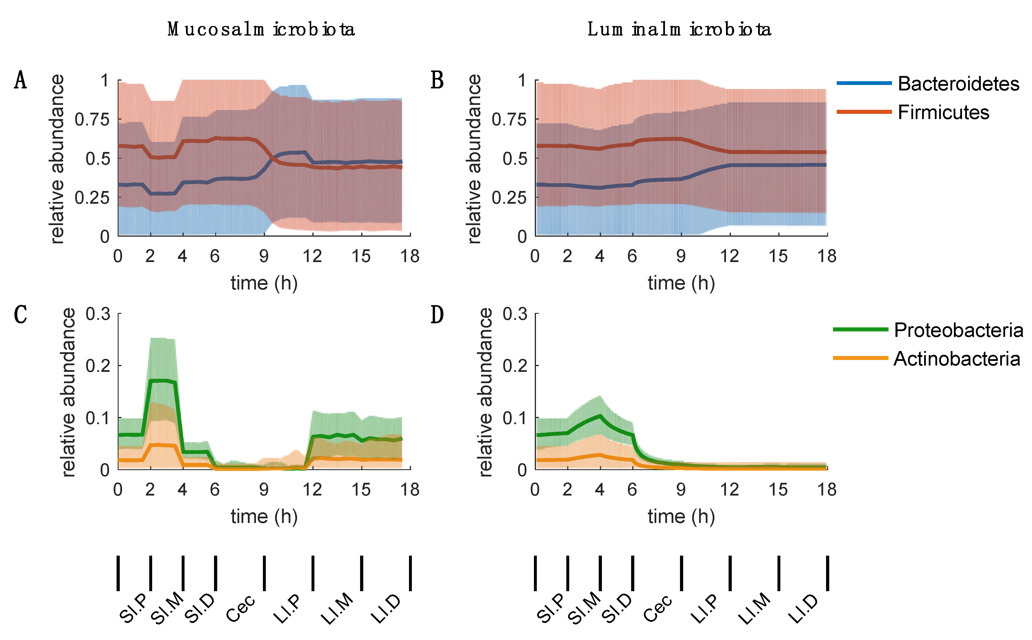
2.5. Inconclusive Firmicutes-to-Bacteroidetes Ratio

While the abundances predicted for aerobes and anaerobes were conserved across randomized uptake parameter simulations, the abundances predicted for Bacteroidetes and Firmicutes did not follow a unique trend (large standard deviations in Figure 3). The Firmicutes-to-Bacteroidetes ratio is known to be variable and may depend on host-specific factors [57]. The inconclusive abundance predictions for Bacteroidetes and Firmicutes may echo their intrinsic variability. Alternatively, the present model is not sufficient to predict at this level of granularity. Note that we only considered B. thetaiotamicron for the phylum Bacteroidetes, F. prausnitzii and E. rectale for Firmicutes, E. coli for Proteobacteria and C. glutamicum for Actinobacteria. Including more microbes such as representatives from Lactobacillales and Bifidobacterium may improve prediction fidelity. Despite its simplicity, the model was sufficient in predicting the change in aerobes and anaerobes in the gut microbiota.

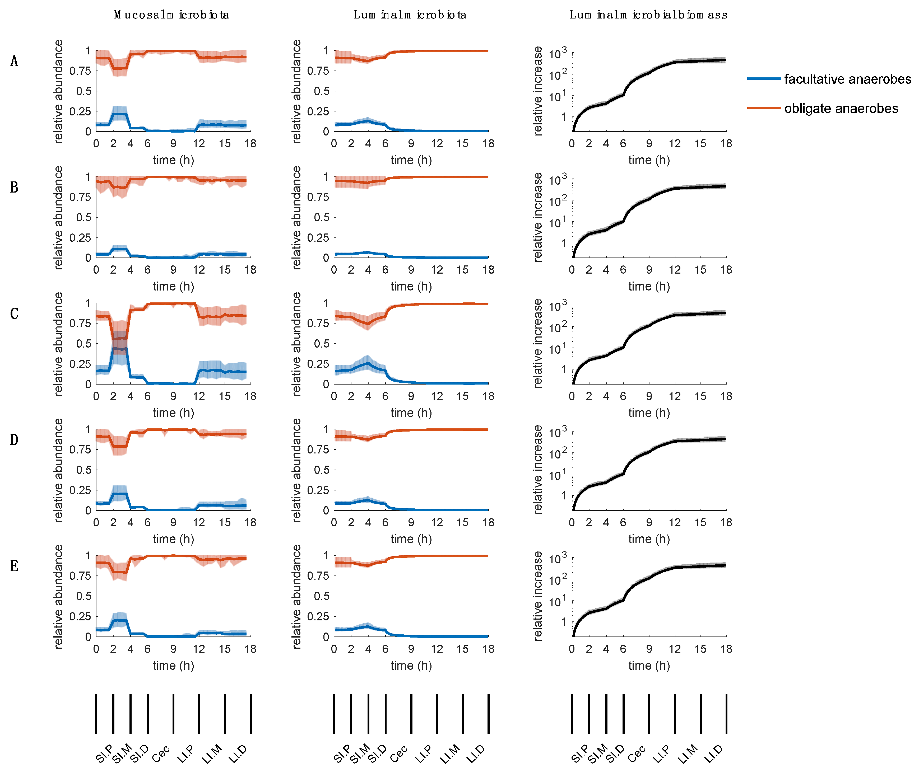
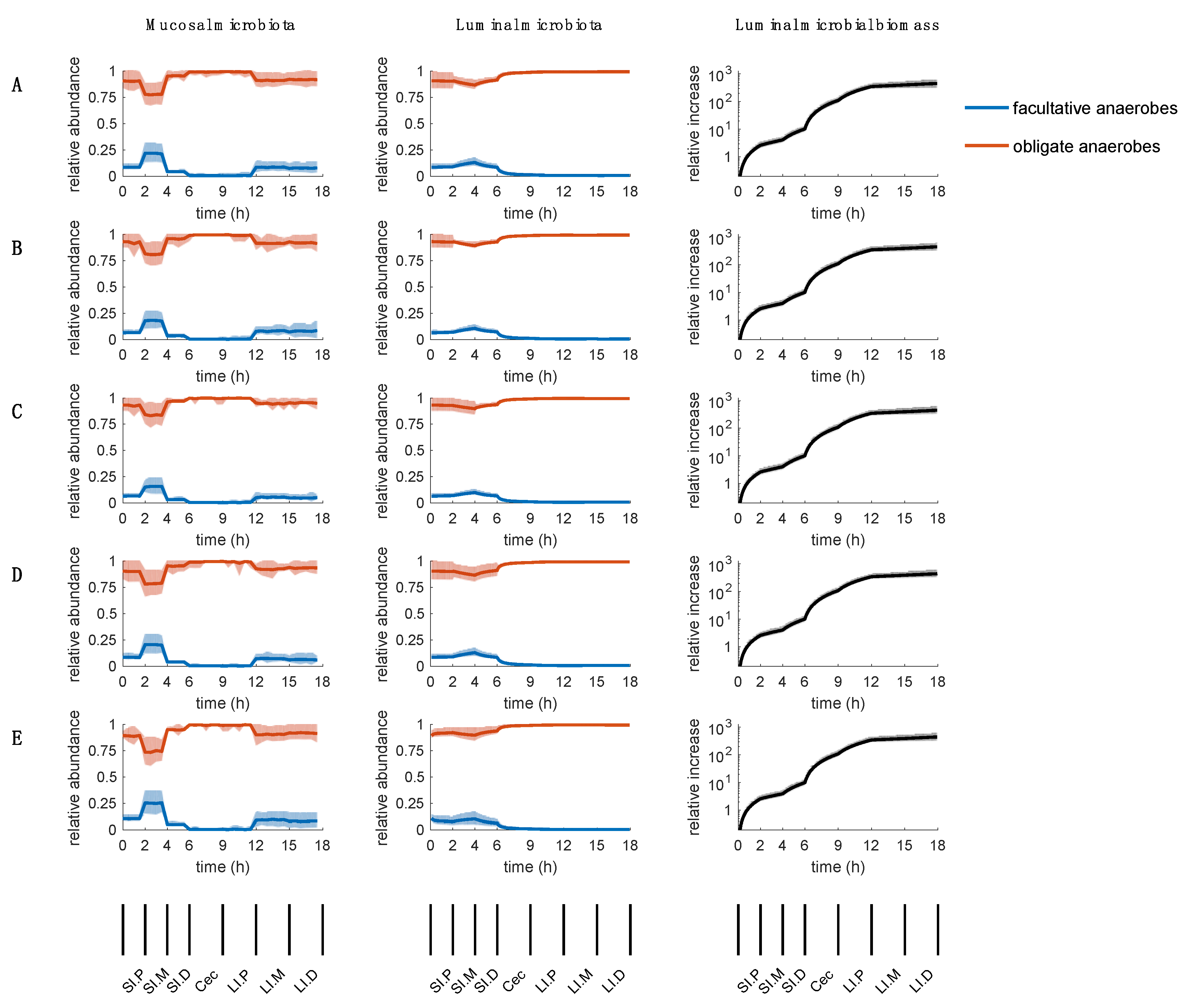
2.6. Sensitivity of Parameters

Parameters $X_{muc}^{total}$, $r_{oxygen}^{total}$ ${\alpha }_{oxygen}^{lum}$, and $L{B}_{OUR}^k$ were varied according to the entries in Table 2, Table 3, Table 4 and Table 5 and the oxygen simulations section. Simulations were repeated for 200 sets of uptake bounds randomly selected from the first simulation. Varying $X_{muc}^{total}$ (i.e., the biomass density of the mucosal microbiota) changed the model prediction most significantly (Figure 4). Setting $X_{muc}^{total}$ uniformly at a low (10⁻⁶ gdw/gram), medium (10⁻⁵) or high (10⁻⁴) level yields results not consistent with the experimental observations. Varying the other three parameters regarding oxygen availability and uptake by aerobes, $r_{oxygen}^{total}$, ${\alpha }_{oxygen}^{lum}$ and $L{B}_{OUR}^k$, though changing the model predictions quantitatively, did not significantly change the overall trends (Figure 5, Figure 6 and Figure 7). Among the three parameters, a 2-fold increase and decrease in the total oxygen available $r_{oxygen}^{total}$ respectively caused relatively more significant quantitative changes (Figure 5).

The sensitivity of $X_{muc}^{total}$ and $r_{oxygen}^{total}$ (Figure 4 and Figure 5) supports the hypothesis that the spatial distribution of aerobes and facultative anaerobes vs. obligate anaerobes in the gut microbiota depends primarily on the oxygen available relative to the microbial population size. To test the impact of oxygen-per-mucosal-biomass availability $r_{oxygen}^{total}/X_{muc}^{total}$ on the spatial distribution, $r_{oxygen}^{total}$ was set to vary in the same order of magnitude as $X_{muc}^{total}$ along the intestines such that $r_{oxygen}^{total}/X_{muc}^{total}$ is constant in each intestinal section in each simulation (see Table 5 for the values). For each value of $r_{oxygen}^{total}/X_{muc}^{total}$ tested, the relative abundances for aerobes and facultative anaerobes vs. obligate anaerobes do not change significantly along the intestines (Figure 8). When $r_{oxygen}^{total}/X_{muc}^{total}$ was 10-fold higher than the default value in the proximal small intestine, facultative anaerobes had an average relative abundance of about 75% (Figure 8A). When $r_{oxygen}^{total}/X_{muc}^{total}$ was equal to the default value in the proximal small intestine, the relative abundance of facultative anaerobes remained at about 10% (Figure 8B), similar to the proximal small intestine simulated under the default condition (Figure 2). As the value was further decreased, close to or smaller than that in the cecum and proximal large intestine, obligate anaerobes dominated (Figure 8C–E). The sensitivity analysis results suggested that the observed large variation in the total mucosal microbial density across various intestinal sections (up to 100-fold difference, Table 1) in conjunction with the comparatively small variation in the oxygen level is the primary factor shaping spatial distribution of aerobes and facultative anaerobes vs. obligate anaerobes.

3. Discussion

3.1. A Dynamic Model Capturing the Spatial Distribution of Aerobes vs Anaerobes

In this study, the established SteadyCom and DMMM microbial metabolism modeling frameworks were used in tandem to predict the steady-state mucosal microbiota and the dynamic luminal microbiota respectively at each time step given the nutrients available. We integrated the algorithms into a population dynamic model by connecting the microbial abundances in the mucosal and luminal microbiota across the intestines. Although the species-level predictions were inconclusive possibly due to the simplified community model consisting of only five microbial species, the model was able to capture the spatial distribution of aerobes and facultative anaerobes vs obligate anaerobes based on the experimental microbial density on the mucus layer and the estimated oxygen consumption rate only [23,24]. The study found that Actinobacteria and Proteobacteria were only present in the luminal and mucosal microbiota in the small intestine, and the mucosal microbiota in the middle and distal large intestine, which is captured qualitatively by our model (Figure 2A–B). This suggests that the genome-scale metabolic modeling approach can reasonably predict oxygen-dependent microbial growth given the nutrients available, which has been demonstrated in previous studies on single organisms [58,59]. The model dynamics assume that the shedding of mucosal microbiota in addition to the luminal microbial growth is an important parameter shaping the luminal microbiota. The predicted accumulation of luminal microbial biomass as a consequence of the hypothesis was similar to the experimental distribution of the luminal microbial biomass. The hypothesis could potentially represent an important interaction between the mucosal and luminal microbiota and is worth further study. The integrated dynamic model could become a valuable tool for exploring therapeutic strategies for site-specific perturbation of the gut microbiota and the associated metabolic activities. For example, perturbing the microbial density on the mucus layer at a site upstream can possibly reshape the microbial abundance at a site downstream.

3.2. Parameters Regarding Oxygen Availability and Uptake

Oxygen availability and uptake was modeled by testing three parameters $r_{oxygen}^{total}$, ${\alpha }_{oxygen}^{lum}$ and $L{B}_{OUR}^k$ instead of directly modeling oxygen diffusion. There are two reasons for this. (1) More physical and kinetic parameters are required. (2) Varying the three oxygen-related parameters currently tested is sufficient to determine the possible behavior of the model. We have estimated the parameters based on the experimental value of microbial oxygen uptake rate and other experimental values reported previously (see SI Methods). Under the present setting, the total oxygen flux available to the microbes for uptake, which changes only among the sections of the intestines, can be regarded as the average oxygen flux available to the microbes over time (mmol h⁻¹) in a certain section of the intestines.

3.3. Potential Future Extension of the Model

The proposed model connecting the steady-state mucosally adherent microbiota and the transient luminal microbiota along various sections of the intestines presents a foundational framework for simulating the gut microbiome dynamics and opens room for refinement and improvement. For example, the model can be further refined by explicitly integrating COMETS [49] or BacArena [52] to model the oxygen, metabolite and microbial cell diffusion processes on the mucus layer and in the lumen if more time-course data of oxygen diffusion and stratified microbial abundance data are available in the future, instead of simply using average oxygen consumption rates as in the current model. In addition to oxygen diffusion, another study reported that in addition to some aerobes and facultative anaerobes, asacharolytic bacteria were also found to be uniquely present in mucosal samples [22]. Their ability to metabolize more proteinaceous substrates such as mucus glycoprotein was suggested to explain this observation, as also simulated in silico previously [52]. The current simulation setting was not able to capture this due to the fact that the metabolic environment in the lumen and on the mucus layer was assumed to be the same except for the oxygen availability, because our aim was to test the impact of oxygen alone. A higher resolution of the microbiome dynamics can be obtained using site-specific metabolic environments and community models encompassing a large number of species.

4. Materials and Methods

4.1. Metabolic Models and Nutrient Availability

The genome-scale metabolic models (GSMs) for five organisms encompassing representative species in the four major phyla among gut microbes were used as proxies for the gut microbiota in each copy of the community metabolic model (Table 1). The GSM models used were all validated and curated in previous publications (see Table 1). The biomass reactions were standardized for community simulation [60]. In particular, a model for Corynebacterium glutamicum was used because Corynebacterium was the only Actinobacteria that was found to be present consistently in mucosal samples and absent in the majority of stool samples in a previous study [22]. Each microbe-specific GSM model within the simulated gut microbiota accounts for all known metabolic reactions carried out by the organism. An aggregate reaction, known as the biomass reaction, represents the accumulation of the metabolites required for growth in their experimentally measured proportions. Pseudo steady-state in metabolism is assumed for each organism resulting in the equal production and consumption of each intracellular metabolite. A community model is formed from multiple organisms by allowing them to compete for or cross-feed metabolites. The nutrients available to the community are defined based on the chemical composition of a mouse chow diet minus the absorption of nutrients by the host (see Table S1 for the detailed estimation). Generally, 99% of carbohydrates, 95% of fatty acids, 95% of amino acids, and 0% of dietary fiber are absorbed by the host, as estimated previously [43,61]. Metabolites are free for exchange between the mucosal and luminal microbiota, except for oxygen.

Table 1. Organisms in the community model.

Organism	Phylum	Ref.
Bacteroides thetaiotaomicron (B. thetaiotaomicron)	Bacteroidetes	[36,38]
Eubacterium rectale (E. rectale)	Firmicutes	[39]
Faecalibacterium prausnitzii (F. prausnitzii)	Firmicutes	[62]
Escherichia coli (E. coli)	Proteobacteria	[63]
Corynebacterium glutamicum (C. glutamicum)	Actinobacteria	[64]

Table 1. Organisms in the community model.

Organism	Phylum	Ref.
Bacteroides thetaiotaomicron (B. thetaiotaomicron)	Bacteroidetes	[36,38]
Eubacterium rectale (E. rectale)	Firmicutes	[39]
Faecalibacterium prausnitzii (F. prausnitzii)	Firmicutes	[62]
Escherichia coli (E. coli)	Proteobacteria	[63]
Corynebacterium glutamicum (C. glutamicum)	Actinobacteria	[64]

4.2. Mucosal Microbiota

The mucosal microbiota is assumed to reach steady-state due to the complete microbial colonization and the relatively stable composition observed [65]. As a result, we used the SteadyCom formulation [43] to predict the composition of the microbial community:

$$\max {\mu }_{muc}^s$$

(1)

subject to

$${\displaystyle \sum }_{j\in J^k}{S}_{ij}^k{V}_j^k=0 \forall i\in I^k,k\in K$$

(2)

$$L{B}_j^k{X}^k\le V_j^k\le U{B}_j^k{X}^k \forall j\in J^k,k\in K$$

(3)

$$V_{biomass}^k={\mu }_{muc}{X}^k \forall k\in K$$

(4)

$$u_i-e_i+{\displaystyle \sum }_{k\in K}{V}_{e{x}^k\left(i\right)}^k=0 \forall i\in I^{com}$$

(5)

$$u_{O_2}=r_{oxygen}^{total,s}\left(1-{\alpha }_{oxygen}^{lum,s}\right)$$

(6)

$${\displaystyle \sum }_{k\in K}{X}^k=X_{muc}^{total,s}$$

(7)

$$\mu ,X^k,e_i\ge 0 \forall i\in I^{com},k\in K$$

(8)

$$V_j^k \mathrm{is}\mathrm{free}\forall j\in J^k,k\in K$$

(9)

where the superscript s represents intestinal section s, $K$ is the set of all organisms (index k), $I^k$ is the set of all metabolites in organism k (index i), $I^{com}$ is the set of all community metabolites shared among the organisms, $J^k$ is the set of all reactions in organism k (index j). $j=e{x}^k\left(i\right)$ is the exchange reaction for community metabolite i of organism k. For exchange reactions, the convention is that positive flux represents the export of the metabolite from the organism to the community and negative represents the uptake of a metabolite by an organism from the community.

The decision variables are described as follows: $X^k$ is the biomass for organism k, in gram dry weight (gdw). ${\mu }_{muc}^s$ is the growth rate of the mucosal microbiota in section s, in h⁻¹. $e_i$ is the export flux of community metabolite i, in mmol h⁻¹. $V_j^k$ is the aggregate flux of reaction j for organism k, in mmol h⁻¹. In particular, $V_{biomass}^k$ is the biomass production rate, which together with the rates for other macromolecular productions in the model, has the unit of gdw h⁻¹.

The parameters are described as follows: $S_{ij}^k$ is the stoichiometry of metabolite i in the reaction j of organism k. $L{B}_j^k$ and $U{B}_j^k$ are the lower and upper bound for the specific rate of reaction j of organism k, in mmol gdw⁻¹h⁻¹, respectively. $u_i$ is the inflow of the community metabolite i, in mmol h⁻¹. $u_i=c_i/\Delta t_{muc}$ in the simulation except for oxygen, where c_i is the concentration of metabolite I and $\Delta t_{muc}$ is the step size of time for successive simulation of the mucosal microbiota. $r_{oxygen}^{total,s}$ is the total oxygen flux from the epithelial cells. ${\alpha }_{oxygen}^{lum,s}$ is the fraction of oxygen flux available to the luminal microbiota after the consumption by the mucosal microbiota. $X_{muc}^{total,s}$ is the total microbial biomass in the mucosal microbiota and has a different value for each section of the intestines based on the experimental biomass density for the mucosal microbiota [24]. Additional alternative sets of values were tested to examine the effect of this parameter on the simulations (Table 2).

Equation (1) maximizes the growth rate of the community so that the predicted community is favored by selection and can act as a reasonable estimate. Equation (2) represents the pseudo steady-state for the intracellular metabolites of each organism. Equation (3) is the flux capacity constraint for each reaction. Equation (4) enforces that the specific growth rate of each organism ($V_{biomass}^k/X^k$) is identical over time. Equation (5) represents the mass balance of the community metabolites shared by the organisms. The total export from the system (e_i) is equal to the sum of the inflow into the system (u_i) and the total consumption (−ve) or production (+ve) by the community. Equation (6) specifies the community uptake rate for oxygen. Equation (7) constrains the total amount of the community biomass. SteadyCom imposes that the averaged specific growth rate over time of each organism is the same. The identical growth rate averaged over time is the steady-state condition when the mucosal microbiota is subject to dilution (due to flushing of luminal contents, shedding of epithelial cells) at a rate assumed to be equal for each microbe (see SI Methods for the detailed derivation and explanation).

Table 2. Sets of values tested for the mucosal biomass density $X_{muc}^{total}$.

${\mathit{X}}_{\mathit{m}\mathit{u}\mathit{c}}^{\mathit{t}\mathit{o}\mathit{t}\mathit{a}\mathit{l}}\left(\mathbf{gdw}{\mathbf{g}}^{-1}\right)$	SI.P	SI.M	SI.D	Cecum	LI.P	LI.M	LI.D
Default	6.75 × 10−6	2.7 × 10−6	1.5 × 10−5	1.95 × 10−4	5.25 × 10−4	7.5 × 10−6	9 × 10−6
Test 1	1 × 10−6	1 × 10−6	1 × 10−6	1 × 10−6	1 × 10−6	1 × 10−6	1 × 10−6
Test 2	1 × 10−5	1 × 10−5	1 × 10−5	1 × 10−5	1 × 10−5	1 × 10−5	1 × 10−5
Test 3	1 × 10−4	1 × 10−4	1 × 10−4	1 × 10−4	1 × 10−4	1 × 10−4	1 × 10−4

Table 2. Sets of values tested for the mucosal biomass density $X_{muc}^{total}$.

${\mathit{X}}_{\mathit{m}\mathit{u}\mathit{c}}^{\mathit{t}\mathit{o}\mathit{t}\mathit{a}\mathit{l}}\left(\mathbf{gdw}{\mathbf{g}}^{-1}\right)$	SI.P	SI.M	SI.D	Cecum	LI.P	LI.M	LI.D
Default	6.75 × 10−6	2.7 × 10−6	1.5 × 10−5	1.95 × 10−4	5.25 × 10−4	7.5 × 10−6	9 × 10−6
Test 1	1 × 10−6	1 × 10−6	1 × 10−6	1 × 10−6	1 × 10−6	1 × 10−6	1 × 10−6
Test 2	1 × 10−5	1 × 10−5	1 × 10−5	1 × 10−5	1 × 10−5	1 × 10−5	1 × 10−5
Test 3	1 × 10−4	1 × 10−4	1 × 10−4	1 × 10−4	1 × 10−4	1 × 10−4	1 × 10−4

4.3. Luminal Microbiota

The microbiota composition and total biomass in the lumen are more variable and thus were modeled to vary over time. The increase in microbial biomass in the luminal contents is driven by two factors in the model: (1) microbes detaching from the mucosal microbiota and (2) the microbial growth of the luminal microbiota (see Figure 1). The biomass detaching from the mucosa is equal to the biomass produced by the mucosal microbiota as predicted by SteadyCom (${\mu }_{muc}^s{X}_{muc}^{k,s}$) since the total biomass of the mucosal microbiota is assumed to be constant over time. The time-dependent growth of the luminal microbiota was predicted using a dynamic framework for microbial communities called Dynamic Multi-species Metabolic Modeling (DMMM) [45]:

$$\max v_{biomass}^k$$

(10)

subject to

$${\displaystyle \sum }_{j\in J^k}{S}_{ij}^k{v}_j^k=0 \forall i\in I^k$$

(11)

$$L{B}_j^k\le v_j^k\le U{B}_j^k \forall j\in J^k$$

(12)

$$v_{e{x}^k\left(i\right)}^k\ge -c_i/\left(X_{lum}^{k,s}\Delta t_{lum}\right) \forall i\in I^{com}$$

(13)

$$v_{O_2}^k\ge -r_{oxygen}^{total,s}{\alpha }_{oxygen}^{lum,s}/X_{lum}^{k,s}$$

(14)

$$v_j^k \mathrm{is}\mathrm{free} \forall j\in J^k$$

(15)

where $c_i$ is concentration of metabolite I, $\Delta t_{lum}$ is the step size of time for successive simulation of the luminal microbiota, and $X_{lum}^{k,s}$ is the biomass of organism k in the lumen. Equations (11)–(12) similar to Equations (2)–(3) represent the pseudo steady-state of intracellular metabolites and the flux capacity constraint respectively. $c_i/\left(X_{lum}^{k,s}\Delta t_{lum}\right)$ is the maximum amount available for uptake in each time-step. The negative sign in Equation (13) is a result of defining the uptake fluxes to be negative in the model. Equation (14) specifies the maximum oxygen uptake rate. Here the flux variable used is $v_j^k$, which is the specific rate of the reaction, in mmol gdw⁻¹h⁻¹.

4.4. Connecting the Luminal and Mucosal Microbiota

For the s-th section of the intestines (s = 1 for proximal small intestine, s = 2 for middle small intestine and vice versa), the overall change in abundance of organism k in the luminal microbiota is given by:

$$\frac{d{X}_{lum}^{k,s}}{d{t}^s}\&={\mu }_{muc}^s{X}_{muc}^{k,s}+{\mu }_{lum}^{k,s}{X}_{lum}^{k,s}, \mathrm{for}{t}^s\in \left[0,T^s\right], \&\forall k\in K , s=1,2,\dots ,7$$

(16)

$$X_{lum}^{k,s}\left(0\right)\&=X_{lum}^{k,s-1}\left(T^{s-1}\right), \forall k\in K , s=1,2,\dots ,7$$

(17)

where ${\mu }_{muc}^s$ and $X_{muc}^{k,s}$ are the growth rate and biomass of organism k on the mucus layer for intestinal section s, respectively. Similarly, ${\mu }_{lum}^{k,s}$ and $X_{lum}^{k,s}$ denote the growth rate and biomass of organism k in the lumen whereas $t^s$ is the time point and $T^s$ is the retention time for intestinal section s. Equation (17) represents the transfer of biomass in the lumen from the upstream section to the current section. The initial microbial biomass in the luminal contents entering into the small intestine from the stomach is assumed to be negligible, compared to the effect of the mucosal microbiota. Therefore, we have $X_{lum}^{k,0}\left(T^0\right)=0$. The concentrations of metabolites in the s-th section of the intestines, $c_i^s$, are updated by the following population balance model:

$$\frac{d{c}_i^s}{d{t}^s}={\displaystyle \sum }_{k\in K}\left(V_{e{x}^k\left(i\right)}^{k,s}+X_{lum}^{k,s}{v}_{e{x}^k\left(i\right)}^{k,s}\right), \mathrm{for}{t}^s\in \left[0,T^s\right] , \forall i\in I^{com}, s=1,2,\dots ,7$$

(18)

$$c_i^s\left(0\right)=c_i^{s-1}\left(T^{s-1}\right) \forall i\in I^{com},s=1,2,\dots ,7$$

(19)

Here $V_{e{x}^k\left(i\right)}^{k,s}$ and $X_{lum}^{k,s}{v}_{e{x}^k\left(i\right)}^{k,s}$ are the fluxes of the exchange of metabolite i due to organism k in the mucosal and luminal microbiota in the s-th section of the intestines, respectively. Both terms are scaled to the abundance of organism k. Equation (19) represents the transfer of metabolites from the upstream section to the current section. The initial concentration profiles, $c_i^0\left(T^0\right)$, is the estimated dietary contents available to the gut microbes. In SteadyCom the aggregate rate $V_j^k$ (in mmol h⁻¹) is used in order to maintain linearity in the optimization model rather than the specific rate $v_j^k$ (in mmol gdw⁻¹h⁻¹) as in DMMM.

4.5. Oxygen Availability

The two separate microbiota (i.e., the mucosal and luminal microbiota) were assumed to share the same extracellular environment for all metabolites except for oxygen. Total oxygen flux availability $r_{oxygen}^{total,s}$ from the epithelial cells and the fraction of oxygen flux available to the luminal microbiota from the epithelial cells, ${\alpha }_{oxygen}^{lum,s}$ were varied along different sections of the intestines to represent the varying oxygen diffusivity. The values were estimated based on experimental data [24] and the characteristics of the intestines (see supplementary methods Text S1). Various sets of values for $r_{oxygen}^{total,s}$, ${\alpha }_{oxygen}^{lum,s}$ as well as the oxygen-per-mucosal-biomass availability $r_{oxygen}^{total,s}/X_{muc}^{total}$ were tested to examine the sensitivity of the model to these parameters (Table 3, Table 4 and Table 5). The maximum specific oxygen uptake rate for individual microbes $L{B}_{OUR}^k$ was estimated to be 2 mmol gdw⁻¹h⁻¹ based on experimentally reported values [59,66,67] and the gut conditions [22]. Values ranging from 1 to 20 mmol gdw⁻¹h⁻¹ were also tested. For each set of values tested, the oxygen flux available within each section of the intestines was assumed to be constant, representing an average over time for the section. See Supplementary Materials Text S1 for a more detailed estimation of the parameters.

Table 3. Sets of values tested for the total oxygen available $r_{oxygen}^{total}$.

${\mathit{r}}_{\mathit{o}\mathit{x}\mathit{y}\mathit{g}\mathit{e}\mathit{n}}^{\mathit{t}\mathit{o}\mathit{t}\mathit{a}\mathit{l}}$ (mmol h−1g−1)	SI.P	SI.M	SI.D	Cecum	LI.P	LI.M	LI.D
Default	1.6 × 10−6	1.6 × 10−6	1.6 × 10−6	1.6 × 10−6	1.6 × 10−6	1.6 × 10−6	1.6 × 10−6
Test 1	0.8 × 10−6	0.8 × 10−6	0.8 × 10−6	0.8 × 10−6	0.8 × 10−6	0.8 × 10−6	0.8 × 10−6
Test 2	3.2 × 10−6	3.2 × 10−6	3.2 × 10−6	3.2 × 10−6	3.2 × 10−6	3.2 × 10−6	3.2 × 10−6
Test 3	1.6 × 10−6	1.52 × 10−6	1.44 × 10−6	1.36 × 10−6	1.28 × 10−6	1.2 × 10−6	1.12× 10−6
Test 4	1.6 × 10−6	1.44 × 10−6	1.28 × 10−6	1.12 × 10−6	0.96 × 10−6	0.8 × 10−6	0.64× 10−6

Table 3. Sets of values tested for the total oxygen available $r_{oxygen}^{total}$.

${\mathit{r}}_{\mathit{o}\mathit{x}\mathit{y}\mathit{g}\mathit{e}\mathit{n}}^{\mathit{t}\mathit{o}\mathit{t}\mathit{a}\mathit{l}}$ (mmol h−1g−1)	SI.P	SI.M	SI.D	Cecum	LI.P	LI.M	LI.D
Default	1.6 × 10−6	1.6 × 10−6	1.6 × 10−6	1.6 × 10−6	1.6 × 10−6	1.6 × 10−6	1.6 × 10−6
Test 1	0.8 × 10−6	0.8 × 10−6	0.8 × 10−6	0.8 × 10−6	0.8 × 10−6	0.8 × 10−6	0.8 × 10−6
Test 2	3.2 × 10−6	3.2 × 10−6	3.2 × 10−6	3.2 × 10−6	3.2 × 10−6	3.2 × 10−6	3.2 × 10−6
Test 3	1.6 × 10−6	1.52 × 10−6	1.44 × 10−6	1.36 × 10−6	1.28 × 10−6	1.2 × 10−6	1.12× 10−6
Test 4	1.6 × 10−6	1.44 × 10−6	1.28 × 10−6	1.12 × 10−6	0.96 × 10−6	0.8 × 10−6	0.64× 10−6

Table 4. Sets of values tested for the fraction of oxygen available to the luminal microbiota ${\alpha }_{oxygen}^{lum}$.

${\mathit{\alpha }}_{\mathit{o}\mathit{x}\mathit{y}\mathit{g}\mathit{e}\mathit{n}}^{\mathit{l}\mathit{u}\mathit{m}}$	SI.P	SI.M	SI.D	Cecum	LI.P	LI.M	LI.D
Default	0.2	0.15	0.15	0.01	0.05	0.05	0
Test 1	0.4	0.3	0.3	0.05	0.1	0.1	0
Test 2	0.4	0.4	0.4	0.4	0.4	0.4	0.4
Test 3	0.2	0.2	0.2	0.2	0.2	0.2	0.2
Test 4	0	0	0	0	0	0	0

Table 4. Sets of values tested for the fraction of oxygen available to the luminal microbiota ${\alpha }_{oxygen}^{lum}$.

${\mathit{\alpha }}_{\mathit{o}\mathit{x}\mathit{y}\mathit{g}\mathit{e}\mathit{n}}^{\mathit{l}\mathit{u}\mathit{m}}$	SI.P	SI.M	SI.D	Cecum	LI.P	LI.M	LI.D
Default	0.2	0.15	0.15	0.01	0.05	0.05	0
Test 1	0.4	0.3	0.3	0.05	0.1	0.1	0
Test 2	0.4	0.4	0.4	0.4	0.4	0.4	0.4
Test 3	0.2	0.2	0.2	0.2	0.2	0.2	0.2
Test 4	0	0	0	0	0	0	0

Table 5. Sets of values tested for the oxygen-per-mucosal-biomass availability$r_{oxygen}^{total}/X_{muc}^{total}$.

${\mathit{r}}_{\mathit{o}\mathit{x}\mathit{y}\mathit{g}\mathit{e}\mathit{n}}^{\mathit{t}\mathit{o}\mathit{t}\mathit{a}\mathit{l}}/{\mathit{X}}_{\mathit{m}\mathit{u}\mathit{c}}^{\mathit{t}\mathit{o}\mathit{t}\mathit{a}\mathit{l}}$ (mmol gdw−1h−1)	SI.P	SI.M	SI.D	Cecum	LI.P	LI.M	LI.D
Default	0.24	0.59	0.11	0.008	0.003	0.21	0.18
Test 1	2.4	2.4	2.4	2.4	2.4	2.4	2.4
Test 2	0.24	0.24	0.24	0.24	0.24	0.24	0.24
Test 3	0.024	0.024	0.024	0.024	0.024	0.024	0.024
Test 4	0.0024	0.0024	0.0024	0.0024	0.0024	0.0024	0.0024
Test 5	0.00024	0.00024	0.00024	0.00024	0.00024	0.00024	0.00024

Table 5. Sets of values tested for the oxygen-per-mucosal-biomass availability$r_{oxygen}^{total}/X_{muc}^{total}$.

${\mathit{r}}_{\mathit{o}\mathit{x}\mathit{y}\mathit{g}\mathit{e}\mathit{n}}^{\mathit{t}\mathit{o}\mathit{t}\mathit{a}\mathit{l}}/{\mathit{X}}_{\mathit{m}\mathit{u}\mathit{c}}^{\mathit{t}\mathit{o}\mathit{t}\mathit{a}\mathit{l}}$ (mmol gdw−1h−1)	SI.P	SI.M	SI.D	Cecum	LI.P	LI.M	LI.D
Default	0.24	0.59	0.11	0.008	0.003	0.21	0.18
Test 1	2.4	2.4	2.4	2.4	2.4	2.4	2.4
Test 2	0.24	0.24	0.24	0.24	0.24	0.24	0.24
Test 3	0.024	0.024	0.024	0.024	0.024	0.024	0.024
Test 4	0.0024	0.0024	0.0024	0.0024	0.0024	0.0024	0.0024
Test 5	0.00024	0.00024	0.00024	0.00024	0.00024	0.00024	0.00024

4.6. Simulation Parameters

In each section of the intestines, using the oxygen parameters defined and given the final simulated luminal biomass and the remaining nutrient pool from the previous section, the growth and composition of the two microbiota were simulated over a time period equal to the estimated transit time. The initial biomass in the luminal contents entering into the proximal small intestine was set to zero and the nutrient pool was set to be equal to the estimated dietary contents available to the gut microbes. At time t, the steady-state mucosal microbiota was simulated by solving SteadyCom. The solution was used from time t to $t+\Delta t_{muc}$ ($\Delta t_{muc}=$ 30 mins). Within this time period, DMMM for simulating the luminal microbiota was solved with a time step of $\Delta t_{lum}$ ($\Delta t_{lum}$ = 5 mins). The solution from DMMM and SteadyCom were used to update the total biomass of microbes in the lumen and the metabolite concentrations in Equations. (1) and (3). Randomized uptake bounds for carbon sources were used in 1000 simulations to assess the sensitivity of microbial abundances at different uptake capacity of carbon sources as performed previously. In addition, parameters $X_{muc}^{total}$, $r_{oxygen}^{total}$, ${\alpha }_{oxygen}^{lum}$ and $L{B}_{OUR}^k$ were also varied (see Table 2, Table 3 and Table 4 and the subsection Oxygen availability) and simulations were repeated for 200 sets of the uptake bounds randomly selected from the 1000 sets of uptake bounds to assess their sensitivities.

4.7. Availability of Data and Materials

The Matlab code and example script is available at https://github.com/shjchan/spatialGut.

References

1. Sommer, F.; Bäckhed, F. The gut microbiota—Masters of host development and physiology. Nat. Rev. Microbiol. 2013, 11, 227–238. [Google Scholar] [CrossRef] [PubMed]
2. Marchesi, J.R.; Adams, D.H.; Fava, F.; Hermes, G.D.A.; Hirschfield, G.M.; Hold, G.; Quraishi, M.N.; Kinross, J.; Smidt, H.; Tuohy, K.M.; et al. The gut microbiota and host health: A new clinical frontier. Gut 2015, 65, 1–10. [Google Scholar] [CrossRef] [PubMed]
3. Jiang, C.; Xie, C.; Lv, Y.; Li, J.; Krausz, K.W.; Shi, J.; Brocker, C.N.; Desai, D.; Amin, S.G.; Bisson, W.H.; et al. Intestine-selective farnesoid X receptor inhibition improves obesity-related metabolic dysfunction. Nat. Commun. 2015, 6, 10166. [Google Scholar] [CrossRef] [PubMed]
4. Zhang, L.; Xie, C.; Nichols, R.G.; Chan, S.H.J.; Jiang, C.; Hao, R.; Smith, P.B.; Cai, J.; Simons, M.N.; Hatzakis, E.; et al. Farnesoid X receptor signaling shapes the gut microbiota and controls hepatic lipid metabolism. MSystems 2016, 1, e00070-16. [Google Scholar] [CrossRef] [PubMed]
5. Bajaj, J.S.; Cox, I.J.; Betrapally, N.S.; Heuman, D.M.; Schubert, M.L.; Ratneswaran, M.; Hylemon, P.B.; White, M.B.; Daita, K.; Noble, N.A.; et al. Systems biology analysis of omeprazole therapy in cirrhosis demonstrates significant shifts in gut microbiota composition and function. AJP Gastrointest. Liver Physiol. 2014, 307, G951–G957. [Google Scholar] [CrossRef] [PubMed] [Green Version]
6. Yoo, D.-H.; Kim, I.S.; Van Le, T.K.; Jung, I.-H.; Yoo, H.H.; Kim, D.-H. Gut microbiota-mediated drug interactions between lovastatin and antibiotics. Drug Metab. Dispos. 2014, 42, 1508–1513. [Google Scholar] [CrossRef]
7. Wilson, I.D.; Nicholson, J.K. Gut microbiome interactions with drug metabolism, efficacy, and toxicity. Transl. Res. 2017, 179, 204–222. [Google Scholar] [CrossRef]
8. De Filippo, C.; Cavalieri, D.; Di Paola, M.; Ramazzotti, M.; Poullet, J.B.; Massart, S.; Collini, S.; Pieraccini, G.; Lionetti, P. Impact of diet in shaping gut microbiota revealed by a comparative study in children from Europe and rural Africa. Proc. Natl. Acad. Sci. USA 2010, 107, 14691–14696. [Google Scholar] [CrossRef] [Green Version]
9. Claesson, M.J.; Jeffery, I.B.; Conde, S.; Power, S.E.; O’Connor, E.M.; Cusack, S.; Harris, H.M.B.; Coakley, M.; Lakshminarayanan, B.; O’Sullivan, O.; et al. Gut microbiota composition correlates with diet and health in the elderly. Nature 2012, 488, 178–184. [Google Scholar] [CrossRef]
10. Wu, G.D.; Chen, J.; Hoffmann, C.; Bittinger, K.; Chen, Y.-Y.; Keilbaugh, S.A.; Bewtra, M.; Knights, D.; Walters, W.A.; Knight, R.; et al. Linking long-term dietary patterns with gut microbial enterotypes. Science 2011, 334, 105–108. [Google Scholar] [CrossRef]
11. Cotillard, A.; Kennedy, S.P.; Kong, L.C.; Prifti, E.; Pons, N.; Le Chatelier, E.; Almeida, M.; Quinquis, B.; Levenez, F.; Galleron, N.; et al. Dietary intervention impact on gut microbial gene richness. Nature 2013, 500, 585–588. [Google Scholar] [CrossRef] [PubMed]
12. Turnbaugh, P.J.; Ridaura, V.K.; Faith, J.J.; Rey, F.E.; Knight, R.; Gordon, J.I. The effect of diet on the human gut microbiome: A metagenomic analysis in humanized gnotobiotic mice. Sci. Transl. Med. 2009, 1, 6ra14. [Google Scholar] [CrossRef] [PubMed]
13. Dhingra, D.; Michael, M.; Rajput, H.; Patil, R.T. Dietary fibre in foods: A review. J. Food Sci. Technol. 2012, 49, 255–266. [Google Scholar] [CrossRef] [PubMed]
14. Wu, G.D.; Compher, C.; Chen, E.Z.; Smith, S.A.; Shah, R.D.; Bittinger, K.; Chehoud, C.; Albenberg, L.G.; Nessel, L.; Gilroy, E.; et al. Comparative metabolomics in vegans and omnivores reveal constraints on diet-dependent gut microbiota metabolite production. Gut 2016, 65, 63–72. [Google Scholar] [CrossRef] [PubMed]
15. Spor, A.; Koren, O.; Ley, R. Unravelling the effects of the environment and host genotype on the gut microbiome. Nat. Rev. Microbiol. 2011, 9, 279–290. [Google Scholar] [CrossRef] [PubMed]
16. Yatsunenko, T.; Rey, F.E.; Manary, M.J.; Trehan, I.; Dominguez-Bello, M.G.; Contreras, M.; Magris, M.; Hidalgo, G.; Baldassano, R.N.; Anokhin, A.P.; et al. Human gut microbiome viewed across age and geography. Nature 2012, 486, 222–228. [Google Scholar] [CrossRef]
17. Liang, X.; Bushman, F.D.; FitzGerald, G.A. Rhythmicity of the intestinal microbiota is regulated by gender and the host circadian clock. Proc. Natl. Acad. Sci. USA 2015, 112, 10479–10484. [Google Scholar] [CrossRef] [Green Version]
18. Jakobsson, H.E.; Jernberg, C.; Andersson, A.F.; Sjölund-Karlsson, M.; Jansson, J.K.; Engstrand, L. Short-term antibiotic treatment has differing long-term impacts on the human throat and gut microbiome. PLoS ONE 2010, 5, e9836. [Google Scholar] [CrossRef]
19. Theriot, C.M.; Koenigsknecht, M.J.; Carlson, P.E.; Hatton, G.E.; Nelson, A.M.; Li, B.; Huffnagle, G.B.Z.; Li, J.; Young, V.B. Antibiotic-induced shifts in the mouse gut microbiome and metabolome increase susceptibility to Clostridium difficile infection. Nat. Commun. 2014, 5, 3114. [Google Scholar] [CrossRef]
20. Eckburg, P.B.; Bik, E.M.; Bernstein, C.N.; Purdom, E.; Dethlefsen, L.; Sargent, M.; Gill, S.R.; Nelson, K.E.; Relman, D.A. Diversity of the human intestinal microbial flora. Science 2005, 308, 1635–1638. [Google Scholar] [CrossRef]
21. Gillevet, P.; Sikaroodi, M.; Keshavarzian, A.; Mutlu, E.A. Quantitative assessment of the human gut microbiome using multitag pyrosequencing. Chem. Biodivers. 2010, 7, 1065–1075. [Google Scholar] [CrossRef] [PubMed]
22. Albenberg, L.; Esipova, T.V.; Judge, C.P.; Bittinger, K.; Chen, J.; Laughlin, A.; Grunberg, S.; Baldassano, R.N.; Lewis, J.D.; Li, H.; et al. Correlation between intraluminal oxygen gradient and radial partitioning of intestinal microbiota. Gastroenterology 2014, 147, 1055–1063. [Google Scholar] [CrossRef] [PubMed]
23. Liang, X.; Bittinger, K.; Li, X.; Abernethy, D.R.; Bushman, F.D.; FitzGerald, G.A. Bidirectional interactions between indomethacin and the murine intestinal microbiota. Elife 2015, 4, 1–22. [Google Scholar] [CrossRef] [PubMed]
24. Friedman, E.S.; Bittinger, K.; Esipova, T.V.; Hou, L.; Chau, L.; Jiang, J.; Mesaros, C.; Lund, P.J.; Liang, X.; FitzGerald, G.A.; et al. Microbes vs. chemistry in the origin of the anaerobic gut lumen. Proc. Natl. Acad. Sci. USA 2018, 115, 4170–4175. [Google Scholar] [CrossRef] [PubMed] [Green Version]
25. Swidsinski, A.; Sydora, B.C.; Doerffel, Y.; Loening-Baucke, V.; Vaneechoutte, M.; Lupicki, M.; Scholze, J.; Lochs, H.; Dieleman, L.A. Viscosity gradient within the mucus layer determines the mucosal barrier function and the spatial organization of the intestinal microbiota. Inflamm. Bowel Dis. 2007, 13, 963–970. [Google Scholar] [CrossRef]
26. Orth, J.D.; Thiele, I.; Palsson, B.Ø. What is flux balance analysis? Nat. Biotechnol. 2010, 28, 245–248. [Google Scholar] [CrossRef] [PubMed]
27. McCloskey, D.; Palsson, B.O.; Feist, A.M. Basic and applied uses of genome-scale metabolic network reconstructions of Escherichia coli. Mol. Syst. Biol. 2014, 9, 661. [Google Scholar] [CrossRef]
28. Mahadevan, R.; Edwards, J.S.; Doyle, F.J. Dynamic flux balance analysis of diauxic growth in Escherichia coli. Biophys. J. 2002, 83, 1331–1340. [Google Scholar] [CrossRef]
29. Varma, A.; Palsson, B.O. Stoichiometric flux balance models quantitatively predict growth and metabolic by-product secretion in wild-type Escherichia coli W3110. Appl. Environ. Microbiol. 1994, 60, 3724–3731. [Google Scholar]
30. Stolyar, S.; Van Dien, S.; Hillesland, K.L.; Pinel, N.; Lie, T.J.; Leigh, J.A.; Stahl, D.A. Metabolic modeling of a mutualistic microbial community. Mol. Syst. Biol. 2007, 3, 92. [Google Scholar] [CrossRef]
31. Klitgord, N.; Segrè, D. Environments that induce synthetic microbial ecosystems. PLoS Comput. Biol. 2010, 6, e1001002. [Google Scholar] [CrossRef] [PubMed]
32. Freilich, S.; Zarecki, R.; Eilam, O.; Segal, E.S.; Henry, C.S.; Kupiec, M.; Gophna, U.; Sharan, R.; Ruppin, E. Competitive and cooperative metabolic interactions in bacterial communities. Nat. Commun. 2011, 2, 589. [Google Scholar] [CrossRef] [PubMed] [Green Version]
33. Zomorrodi, A.R.; Maranas, C.D. OptCom: A multi-level optimization framework for the metabolic modeling and analysis of microbial communities. PLoS Comput. Biol. 2012, 8, e1002363. [Google Scholar] [CrossRef] [PubMed]
34. Khandelwal, R.A.; Olivier, B.G.; Röling, W.F.M.; Teusink, B.; Bruggeman, F.J. Community flux balance analysis for microbial consortia at balanced growth. PLoS ONE 2013, 8, e64567. [Google Scholar] [CrossRef] [PubMed]
35. Zelezniak, A.; Andrejev, S.; Ponomarova, O.; Mende, D.R.; Bork, P.; Patil, K.R. Metabolic dependencies drive species co-occurrence in diverse microbial communities. Proc. Natl. Acad. Sci. USA 2015, 112, 6449–6454. [Google Scholar] [CrossRef] [PubMed] [Green Version]
36. Heinken, A.; Sahoo, S.; Fleming, R.M.T.; Thiele, I. Systems-level characterization of a host-microbe metabolic symbiosis in the mammalian gut. Gut Microbes 2013, 4, 28–40. [Google Scholar] [CrossRef] [PubMed] [Green Version]
37. Heinken, A.; Thiele, I. Anoxic conditions promote species-specific mutualism between gut microbes in silico. Appl. Environ. Microbiol. 2015, 81, 4049–4061. [Google Scholar] [CrossRef] [PubMed]
38. Heinken, A.; Thiele, I. Systematic prediction of health-relevant human-microbial co-metabolism through a computational framework. Gut Microbes 2015, 6, 120–130. [Google Scholar] [CrossRef]
39. Shoaie, S.; Karlsson, F.; Mardinoglu, A.; Nookaew, I.; Bordel, S.; Nielsen, J. Understanding the interactions between bacteria in the human gut through metabolic modeling. Sci. Rep. 2013, 3, 2532. [Google Scholar] [CrossRef]
40. Shoaie, S.; Ghaffari, P.; Kovatcheva-Datchary, P.; Mardinoglu, A.; Sen, P.; Pujos-Guillot, E.; de Wouters, T.; Juste, C.; Rizkalla, S.; Chilloux, J.; et al. Quantifying diet-induced metabolic changes of the human gut microbiome. Cell Metab. 2015, 22, 320–331. [Google Scholar] [CrossRef]
41. Mardinoglu, A.; Shoaie, S.; Bergentall, M.; Ghaffari, P.; Zhang, C.; Larsson, E.; Backhed, F.; Nielsen, J. The gut microbiota modulates host amino acid and glutathione metabolism in mice. Mol. Syst. Biol. 2015, 11, 834. [Google Scholar] [CrossRef] [PubMed]
42. Magnúsdóttir, S.; Heinken, A.; Kutt, L.; Ravcheev, D.A.; Bauer, E.; Noronha, A.; Greenhalgh, K.; Jäger, C.; Baginska, J.; Wilmes, P.; et al. Generation of genome-scale metabolic reconstructions for 773 members of the human gut microbiota. Nat. Biotechnol. 2016, 35, 81–89. [Google Scholar] [CrossRef] [PubMed]
43. Chan, S.H.J.; Simons, M.N.; Maranas, C.D. SteadyCom: Predicting microbial abundances while ensuring community stability. PLoS Comput. Biol. 2017, 13, e1005539. [Google Scholar] [CrossRef] [PubMed]
44. Henson, M.A.; Phalak, P. Suboptimal community growth mediated through metabolite crossfeeding promotes species diversity in the gut microbiota. PLoS Comput. Biol. 2018, 14, 1–21. [Google Scholar] [CrossRef] [PubMed]
45. Zhuang, K.; Izallalen, M.; Mouser, P.; Richter, H.; Risso, C.; Mahadevan, R.; Lovley, D.R. Genome-scale dynamic modeling of the competition between Rhodoferax and Geobacter in anoxic subsurface environments. ISME J. 2011, 5, 305–316. [Google Scholar] [CrossRef] [PubMed]
46. Hanly, T.J.; Henson, M.A. Dynamic flux balance modeling of microbial co-cultures for efficient batch fermentation of glucose and xylose mixtures. Biotechnol. Bioeng. 2011, 108, 376–385. [Google Scholar] [CrossRef] [PubMed]
47. Zomorrodi, A.R.; Islam, M.M.; Maranas, C.D. d-OptCom: Dynamic multi-level and multi-objective metabolic modeling of microbial communities. ACS Synth. Biol. 2014, 3, 247–257. [Google Scholar] [CrossRef] [PubMed]
48. Wilken, S.; Saxena, M.; Petzold, L.; O’Malley, M. In silico identification of microbial partners to form consortia with anaerobic fungi. Processes 2018, 6, 7. [Google Scholar] [CrossRef]
49. Harcombe, W.R.; Riehl, W.J.; Dukovski, I.; Granger, B.R.; Betts, A.; Lang, A.H.; Bonilla, G.; Kar, A.; Leiby, N.; Mehta, P.; et al. Metabolic resource allocation in individual microbes determines ecosystem interactions and spatial dynamics. Cell Rep. 2014, 7, 1104–1115. [Google Scholar] [CrossRef]
50. Van Hoek, M.J.A.; Merks, R.M.H. Emergence of microbial diversity due to cross-feeding interactions in a spatial model of gut microbial metabolism. BMC Syst. Biol. 2017, 11, 56. [Google Scholar] [CrossRef]
51. Henson, M.; Phalak, P. Byproduct cross feeding and community stability in an in silico biofilm model of the gut microbiome. Processes 2017, 5, 13. [Google Scholar] [CrossRef]
52. Bauer, E.; Zimmermann, J.; Baldini, F.; Thiele, I.; Kaleta, C. BacArena: Individual-based metabolic modeling of heterogeneous microbes in complex communities. PLoS Comput. Biol. 2017, 13, 1–22. [Google Scholar] [CrossRef] [PubMed]
53. Phalak, P.; Chen, J.; Carlson, R.P.; Henson, M.A. Metabolic modeling of a chronic wound biofilm consortium predicts spatial partitioning of bacterial species. BMC Syst. Biol. 2016, 10, 90. [Google Scholar] [CrossRef] [PubMed]
54. Song, H.S.; Cannon, W.; Beliaev, A.; Konopka, A. Mathematical modeling of microbial community dynamics: A methodological review. Processes 2014, 2, 711–752. [Google Scholar] [CrossRef]
55. Van der Ark, K.C.H.; van Heck, R.G.A.; Martins Dos Santos, V.A.P.; Belzer, C.; de Vos, W.M. More than just a gut feeling: Constraint-based genome-scale metabolic models for predicting functions of human intestinal microbes. Microbiome 2017, 5, 78. [Google Scholar] [CrossRef] [PubMed]
56. Magnúsdóttir, S.; Thiele, I. Modeling metabolism of the human gut microbiome. Curr. Opin. Biotechnol. 2018, 51, 90–96. [Google Scholar] [CrossRef] [PubMed]
57. Canfora, E.E.; Jocken, J.W.; Blaak, E.E. Short-chain fatty acids in control of body weight and insulin sensitivity. Nat. Rev. Endocrinol. 2015, 11, 577–591. [Google Scholar] [CrossRef]
58. Fong, S.S.; Marciniak, J.Y.; Palsson, B.O. Description and interpretation of adaptive evolution of Escherichia coli K-12 MG1655 by using a genome-scale in silico metabolic model. J. Bacteriol. 2003, 185, 6400–6408. [Google Scholar] [CrossRef]
59. Ibarra, R.U.; Edwards, J.S.; Palsson, B.O. Escherichia coli K-12 undergoes adaptive evolution to achieve in silico predicted optimal growth. Nature 2002, 420, 186–189. [Google Scholar] [CrossRef]
60. Chan, S.H.J.; Cai, J.; Wang, L.; Simons-Senftle, M.N.; Maranas, C.D. Standardizing biomass reactions and ensuring complete mass balance in genome-scale metabolic models. Bioinformatics 2017, 33, 3603–3609. [Google Scholar] [CrossRef]
61. Rose, C.; Parker, A.; Jefferson, B.; Cartmell, E. The characterization of feces and urine: A review of the literature to inform advanced treatment technology. Crit. Rev. Environ. Sci. Technol. 2015, 45, 1827–1879. [Google Scholar] [CrossRef] [PubMed]
62. Heinken, A.; Khan, M.T.; Paglia, G.; Rodionov, D.A.; Harmsen, H.J.M.; Thiele, I. Functional metabolic map of Faecalibacterium prausnitzii, a beneficial human gut microbe. J. Bacteriol. 2014, 196, 3289–3302. [Google Scholar] [CrossRef] [PubMed]
63. Orth, J.D.; Conrad, T.M.; Na, J.; Lerman, J.A.; Nam, H.; Feist, A.M.; Palsson, B.Ø. A comprehensive genome-scale reconstruction of Escherichia coli metabolism 2011. Mol. Syst. Biol. 2011, 7, 535. [Google Scholar] [CrossRef] [PubMed]
64. Kjeldsen, K.R.; Nielsen, J. In silico genome-scale reconstruction and validation of the Corynebacterium glutamicum metabolic network. Biotechnol. Bioeng. 2009, 102, 583–597. [Google Scholar] [CrossRef] [PubMed]
65. Faith, J.J.; Guruge, J.L.; Charbonneau, M.; Subramanian, S.; Seedorf, H.; Goodman, A.L.; Clemente, J.C.; Knight, R.; Heath, A.C.; Leibel, R.L.; et al. The long-term stability of the human gut microbiota. Science 2013, 341, 1237439. [Google Scholar] [CrossRef]
66. Kiefer, P.; Heinzle, E.; Wittmann, C. Influence of glucose, fructose and sucrose as carbon sources on kinetics and stoichiometry of lysine production by Corynebacterium glutamicum. J. Ind. Microbiol. Biotechnol. 2002, 28, 338–343. [Google Scholar] [CrossRef] [PubMed]
67. Shinfuku, Y.; Sorpitiporn, N.; Sono, M.; Furusawa, C.; Hirasawa, T.; Shimizu, H. Development and experimental verification of a genome-scale metabolic model for Corynebacterium glutamicum. Microb. Cell Fact. 2009, 8, 43. [Google Scholar] [CrossRef]
Figure 1. Proposed dynamic framework for predicting the mucosal and luminal microbiota along various sections of the intestines. (A) Five processes being modeled in each section: (I) the luminal contents at the beginning of the simulation for each section are equal to the luminal contents at the end of the simulation for the previous section. Metabolites in the luminal contents shared freely by the mucosal and luminal microbiota, (II) oxygen diffused from intestinal epithelial cells to the mucus layer and further to the lumen, (III) the metabolism and abundance profile of the luminal microbiota predicted using DMMM, (IV) the metabolism and abundance profile of the mucosal microbiota predicted using SteadyCom, (V) newly produced mucosal microbial biomass shed into the lumen and becoming luminal biomass. (B) The corresponding simulation procedure. The luminal and mucosal microbiota in each section use the same copy of community metabolic network structure consisting of the organisms listed in Table 1.
Processes 07 00394 g001
Figure 2. Simulated microbial abundance (lines) compared with experimentally determined microbial abundance (circles, from reference [24]) at various sections of the intestines in terms of facultative anaerobes vs obligate anaerobes. (A) Abundance profile for the mucosal microbiota. (B) Abundance profile for the luminal microbiota. (C) Relative increase in the luminal microbial biomass. The geometric mean of the luminal microbial biomass for all simulated time points in the first intestinal section (SI.P) was taken as the reference level. The shaded regions and the error bars in all plots represent one standard deviation. The markers at the bottom show the time intervals for which simulations of the corresponding intestinal sections were performed. SI.P, SI.M and SI.D stand for proximal, middle and distal small intestine respectively. Cec stands for cecum. LI.P, LI.M and LI.D stand for proximal, middle and distal large intestine, respectively.
Processes 07 00394 g002
Figure 3. Simulated relative abundance profiles for the four phyla Bacteroidetes, Firmicutes, Actinobacteria and Proteobacteria in the gut community model. Relative abundances for Bacteroidetes and Firmicutes (A) on the mucus layer and (B) in the lumen. Relative abundances for Proteobacteria and Actinobacteria (C) on the mucus layer and (D) in the lumen. The shaded regions in all plots represent one standard deviation. The markers at the bottom show the time intervals for which simulations of the corresponding intestinal sections were performed. SI.P, SI.M and SI.D stand for proximal, middle and distal small intestine respectively. Cec stands for cecum. LI.P, LI.M and LI.D stand for proximal, middle and distal large intestine, respectively.
Processes 07 00394 g003
Figure 4. Varying the biomass density of the mucosal microbiota X m u c t o t a l as detailed in Table 2. (A) Default, experimental values, ranging from ~10−6 to ~10−4. (B) Test 1, constantly 10−6 gdw g−1. (C) Test 2, constantly 10−5 gdw g−1. (D) Test3, constantly 10−4 gdw g−1.
Processes 07 00394 g004
Figure 5. Varying the total oxygen available to the gut microbiota r o x y g e n t o t a l as detailed in Table 3. (A) Default, 1.6 × 10⁻⁶ mmol h−1g−1. (B) Test 1, 0.8 × 10⁻⁶ mmol h−1g−1. (C) Test 2, 3.2 × 10⁻⁶ mmol h−1g−1. (D) Test 3, uniformly decreasing from 1.6 × 10⁻⁶ to 1.12 × 10⁻⁶ mmol h−1g−1. (E) Test 4, uniformly decreasing from 1.6 × 10⁻⁶ to 0.64 × 10⁻⁶ mmol h−1g−1.
Processes 07 00394 g005
Figure 6. Varying the fraction of the total oxygen available to luminal microbiota α o x y g e n l u m as detailed in Table 4. (A) Default, decreasing from 0.2 to 0. (B) Test 1, decreasing from 0.4 to 0. (C) Test 2, constantly 0.4. (D) Test 3, constantly 0.2. (E) Test 4, constantly 0.
Processes 07 00394 g006
Figure 7. Varying the maximum specific oxygen uptake rates of aerobes, L B O U R k . (A) 2 mmol gdw−1h−1, the default value. (B) 1 mmol gdw−1h−1. (C) 5 mmol gdw−1h−1. (D) 10 mmol gdw−1h−1. (E) 20 mmol gdw−1h−1.
Processes 07 00394 g007
Figure 8. Varying the total oxygen available to the gut microbiota r o x y g e n t o t a l such that the oxygen-per-mucosal-biomass availability r o x y g e n t o t a l / X m u c t o t a l remains constant along the intestines in each simulation as detailed in Table 4. (A) 2.4   mmol   gdw 1 h 1 . (B) 0.24   mmol   gdw 1 h 1 , same as the default value in the proximal small intestine. (C) 0.024   mmol   gdw 1 h 1 . (D) 0.0024   mmol   gdw 1 h 1 , close to the default value in the proximal large intestine. (E) 0.00024   mmol   gdw 1 h 1 .
Processes 07 00394 g008