Optimization-Based Scheduling for the Process Industries: From Theory to Real-Life Industrial Applications


1
Department of Chemical Engineering, Aristotle University of Thessaloniki, 54124 Thessaloniki, Greece
2
Chemical Process and Energy Resources Institute (CPERI), Centre for Research and Technology Hellas (CERTH), P.O. Box 60361, 57001 Thessaloniki, Greece
*
Author to whom correspondence should be addressed.
Processes 2019, 7(7), 438; https://0-doi-org.brum.beds.ac.uk/10.3390/pr7070438
Submission received: 27 May 2019
/
Revised: 2 July 2019
/
Accepted: 4 July 2019
/
Published: 10 July 2019
(This article belongs to the Special Issue Commemorative Issue to Celebrate the Life and Work of Prof. Roger W.H. Sargent)
Abstract
:Scheduling is a major component for the efficient operation of the process industries. Especially in the current competitive globalized market, scheduling is of vital importance to most industries, since profit margins are miniscule. Prof. Sargent was one of the first to acknowledge this. His breakthrough contributions paved the way to other researchers to develop optimization-based methods that can address a plethora of process scheduling problems. Despite the plethora of works published by the scientific community, the practical implementation of optimization-based scheduling in industrial real-life applications is limited. In most industries, the optimization of production scheduling is seen as an extremely complex task and most schedulers prefer the use of a simulation-based software or manual decision, which result to suboptimal solutions. This work presents a comprehensive review of the theoretical concepts that emerged in the last 30 years. Moreover, an overview of the contributions that address real-life industrial case studies of process scheduling is illustrated. Finally, the major reasons that impede the application of optimization-based scheduling are critically analyzed and possible remedies are discussed.
1. Introduction
Scheduling is concerned with the allocation of scarce resources among competing activities over time. It is a decision-making process aiming to optimize one or more objectives by taking into account the processes taking place and their interactions with the environment. Scheduling problems exist in many manufacturing and production systems, in transportation and distribution of people and goods, and in other types of industries. The three elements which need to be mapped out are time, tasks and resources: The time at which the tasks have to be performed needs to be optimized considering the availability and restrictions on the required resources. The resources may include processing, material storage and transportation equipment, manpower, utilities (e.g., steam, electricity), any supplementary equipment and so on. The tasks typically include processing operations (e.g., reaction, separation, blending, packaging) as well as other activities like transportation, cleaning in place, changeovers, etc. Both external and internal elements of the production need to be considered. The external element originates from the need to co-ordinate manufacturing and inventory levels based on a given demand, as well as arrival time of raw materials and even maintenance activities. The internal element considers the execution of tasks in an appropriate sequence and time, while taking into account all external considerations and resource availabilities. Overall, the sequencing and timing of tasks over time and the assignment of appropriate resources to the tasks must be performed in an efficient manner, that will, as far as possible, optimize an objective. Typical objectives include the minimization of cost or maximization of profit, the maximization of throughput, the minimization of tardy jobs, etc.
Flexible multipurpose plants are able to produce a wide range of different products using a variety of production routes. This characteristic makes such plants particularly effective for the manufacture of classes of products that exhibit a large degree of diversity and which are subject to fast-varying demands. Due to their inherent flexibility, the scheduling of such plants is a problem of high complexity. Compared to other parts of the supply chain management (e.g., distribution management and inventory control), the production scheduling is often by far the most computationally demanding part. The most general “multipurpose” plants can be viewed as collections of production resources (e.g., raw materials, processing and storage equipment, utilities, manpower) shared by a number of processing operations manufacturing a number of products over a given time horizon. The process may involve intermediates shared among two or more products, recycles of unconverted material, and multiple routes to the same end product. Single or multiple stage multi-product plants are thus special cases of multipurpose plants.
Roger Sargent was one of the first researchers in chemical engineering who foresaw the value of, and need for optimization in the design, control, and operation of process systems. One of the major steps in his research was in the area of multipurpose batch and continuous process scheduling, where the introduction of the state-task network (STN) concept was a major breakthrough. This generic representation allowed researchers to efficiently address arbitrary configurations of recipe-based batch operations. The major novelty was that equipment was not preassigned, like in previous contributions [1]. The utilization of the STN representations for the production scheduling problem resulted to a discrete time mixed-integer linear programming (MILP) model. Despite its novelty, that paper was rejected twice, since at that time MILP algorithms were considered inefficient and incapable of solving large-scale problems, which of course has changed drastically over the last decades [2]. Furthermore, progress with the STN modelling approach was also due to the improved formulation proposed by Nilay Shah in which big-M constraints were replaced by fewer and tighter sets of constraints [3].
An indicative example of the impact of Sargent’s research work in the process scheduling area is his paper, “A General Algorithm for Short-Term Scheduling of Batch-Operations. 1. MILP Formulation” by E. Kondili, C. C. Pantelides, and R. W. H. Sargent, Computers & Chemical Engineering, 17, 211–227 (1993). This is one of the most widely cited contributions in the PSE (Process Systems Engineering) community (over 800 citations in SCOPUS as of April 2019), and has been recognized by researchers all over the world as the major framework for mathematically modeling batch and continuous operations through the state-task-network representation.
The formulation of Kondili et al. [4] relies on binary variables that specify whether a task starts in an equipment at the start of each time period. Other key variables denote the amount of material in each state, and the amount of utility required for processing tasks over each time interval. Equipment and utility usage constraints as well as material balances and capacity constraints are considered in the formulation. A common, discrete time grid is employed to capture all plant resource utilizations in a straightforward manner. This approach was hindered in its ability to handle large problems mainly due to the limitations of discrete-time approaches that require relatively large numbers of grid points, thus resulting to large-sized models.
Inspired by the work of Kondili et al. [1] a number of contributions appeared in the literature utilizing the STN representation and the overall mathematical programming framework to address general classes of batch and continuous process scheduling problems. Shah et al. [3] was able to generate the smallest possible integrality gap for this type of formulation by efficiently modifying the allocation constraints. They additionally proposed a tailored branch-and-bound solution procedure that uses a significantly smaller LP (Linear Programming) relaxation in order to further improve integrality at each node. In the same research, authors addressed the cyclic scheduling problem, where they simultaneously derived optimal schedules as well as the frequency at which they should be repeated [5]. Papageorgiou and Pantelides [6,7] further expanded this work to cover the case of multiple campaigns. Yee and Shah [8,9] also considered variable elimination to improve the performance of general discrete-time scheduling models. More specifically, they recognized that only about 5–15% of the variables are active at the integer solution, and it would be beneficial to identify and eliminate as far as possible inactive variables prior to solving the scheduling problem. To achieve that, they introduce an LP-based heuristic, alongside a flexibility and sequence reduction technique and a formal branch-and-price method.
Pantelides et al. [10] presented an STN-based approach for the scheduling problem of pipeless plants, where material is transferred between processing stations in vessels, thus requiring the simultaneous scheduling of the movement and processing operations. Pantelides [11] criticized the STN, arguing that despite its advantages, it inherently suffers from a number of drawbacks. For example, the fact that each equipment if treated as a distinct entity that results to solution degeneracy in case of multiple equivalent items exist. Therefore, he proposed a differentiated representation, the resource-task network (RTN), which is based on the equable description of all resources [11]. Contrary to the STN representation, where different states are consumed or produced by a task utilizing the equipment and the utilities, in this approach even the items of equipment or the plants’ utilities are considered as resources. Production units are assumed to be consumed at the start and produced at the end of a task. Furthermore, different equipment conditions (e.g., “clean” or “dirty”) can be treated as separate resources, with different activities (e.g., “processing” or “cleaning”) consuming and generating them—this allows for a simple representation of changeovers. Pantelides illustrated that the integrality gap of RTN formulations is never worse than the most efficient form of STN formulation, and the ability to adapt additional problem features in a straightforward way, made it a favorable framework for future research.
The review above has mainly focused on the development of discrete-time models. As pointed out by Schilling [12], while discrete-time models have been capable to handle numerous industrially-relevant problems (see, e.g., [13]), they are characterized by a number of inherent drawbacks:
- A large number of time periods is required to capture all significant events and extract a high quality solution—this usually results to extremely large models;
- Operations in which the processing time is dependent on the batch size are difficult to be modelled;
- The modelling of continuous and semi-continuous operations must be approximately modelled.
In order to address these issues a number of researchers have attempted to develop scheduling models that employ a continuous representation of time. As a result, fewer grid points are required leading to fewer variables and smaller model sizes.
Dimitriadis et al. [14] describe two rolling horizon procedures for medium-term planning and scheduling, based on the more general RTN formulation. They take advantage of the unique properties of Wilkinson et al. [15] and aggregation in this context. In the forwards rolling horizon algorithm, the horizon is divided into two-time blocks. The first is relatively short and modelled in detail, while the second is relatively long and modelled using the aggregate scheduling formulation. The solution of this MILP gives rise to a detailed solution for the first period and an aggregate one for the second. Dimitriadis et al. [14] recognized that, rather than fix all the variables in the first period at the next iteration of the procedure, it makes sense only to fix the complicating integer variables and leave the continuous ones free for further optimization. At the next iteration, there are three time blocks, the first one with fixed integer variables, the second one modelled in detail and the third (the remainder of the horizon) modelled at an aggregate level. The algorithm proceeds until a detailed solution is obtained for the entire horizon.
As noted in the excellent review by Shah [16] a common conclusion in most PSE contributions is that one of the most important advances in the area of process scheduling over the past 25 years has been the increasing usage of rigorous mathematical programming approaches. In addition, the importance of the establishment of frameworks for process scheduling which can be used for the description of a wide variety of processes and for the development of general solution algorithms has been emphasized.
The contributions described above, inspired many researchers from the PSE community to further investigate the production scheduling problem. Numerous novel approaches have been proposed by different research teams, providing novel efficient models and solution techniques. Network representations [17], event-based formulations [18] and precedence-based models [19] have been developed. Furthermore, a high interest has been expressed for real-life industrial study cases and problem specific solutions have been generated for real industrial facilities. Moreover, the ever-increasing computational power, allowed the handling of larger problem instances. However, there is still a significant gap between the academic research and the industrial practice, as only a few contributions have been successfully applied in real-life scheduling problems.
The rest of this paper is organized as follows. In Section 2, a detailed analysis of the theoretical concepts of optimization-based process scheduling is presented, including a classification of the different mathematical models, as well as a characterization of the problems they are able to address. Section 3 illustrates a systematic review on the application of optimization methods in real-life industrial scheduling problems in the process industries. The main modelling features and the industrial case study characteristics are summarized. In Section 4, we highlight the major challenges in applying optimization methods in real industrial problems and discuss potential remedies to close the existing gap between theoretical advancements and practical implementations. Finally, Section 5, draws up the main concluding remarks of this work
2. Theoretical Aspects of Optimization-Based Process Scheduling
As noted by Gabow [20], all scheduling problems are NP-hard, meaning that no known solution algorithms exist that are of polynomial complexity in the problem size. Therefore, the development of efficient optimization-based solution strategies for production scheduling has been a great challenge to the research community. As a result, a significant contribution emerged in the last decades aiming to develop either tailored algorithms for specific problem instances or efficient generic methods.
2.1. Classification of Scheduling Problems
Main goal of all scheduling problems is to propose a schedule that reaches the production targets, while respecting all operational, logistical and technical constraints, and achieves a certain objective, such as the maximization of profit, the minimization of the total cost, earliness and/or tardiness, and production makespan.
The general scheduling problem seeks to optimally answer the following questions (Figure 1):
- What tasks must be executed to satisfy the given demand (batching/lot-sizing)?
- How should the given resources be utilized (task-resource assignment)?
- In what order are batches/lots processed (sequencing and/or timing)?
Note that depending on the specifics of the problem in hand, some of these decisions are not considered in the scheduling level. When developing a model for the optimal scheduling all characteristics of the production must be considered to ensure the feasibility of the proposed schedules. However, the production needs to be portrayed in an abstract way to reduce the computational complexity of the problem. This is even more crucial when dealing with real-life industrial applications, which are typically characterized by complex structures, ever-expanding product portfolios and a huge number of constraints that must be considered.
Traditionally, scheduling problems are defined in terms of a triplet α/β/γ [21]. The α field describes the production environment, while the β field denotes the special characteristics and production constraints. Finally, field γ describes the problem’s objective, e.g., minimization of cost. The entries of this triplet can be extremely diverse between process industries, since a great variety of aspects needs to be considered when developing optimization models for process scheduling. As a result, many classes of scheduling problems exist. However, the general production scheduling problem can be summarized as follows:
- Facility data; e.g., processing stages and units, storage vessels, processing rates, unit to task compatibility.
- Production targets that need to be satisfied.
- Availability of raw materials and resource limitations; e.g., maintenance of units, availability of utilities.
The first term denotes the characteristics of the facility and can be considered static input to the scheduling problem, since it remains the same for all problem instances of a facility, unless any redesign studies are considered. The remaining terms are inputs from other decision-making processes in the manufacturing environment. Scheduling is not a standalone problem; it is part of the manufacturing supply chain and has strong connections to other planning functions. Production targets and materials availability come from the planning level, while resource availability is an output of the control level, thus there is a significant flow of information from other planning functions to scheduling (Figure 2).
Scheduling is a critical decision-making process in all process industries, from the chemical and pharmaceutical to the food and beverage and the petrochemical sector. Besides the aforementioned general description of scheduling, industrial applications display strong differences to each other, due to the facility itself, the production policy or market and business considerations. First step when approaching an industrial scheduling problem is to identify its problem specifics, in order to accurately portray the problem in hand. Moreover, a strong correlation between different classes of scheduling problems and the available mathematical modelling frameworks exist. The scheduling problems found in process industries are classified in terms of: (a) The production facility, (b) the interaction with the rest of the production supply chain, and (c) the specific processing characteristics and constraints. A short description of these terms follows, the interested reader can find details in the excellent reviews of Maravelias [22] and Harjunkoski et al. [23].
2.1.1. The Production Facility
At this point we should note that the following analysis focuses on production scheduling. However, many scheduling problems in the process industries target to the optimization of material transfer operations rather than production operations. Characteristic examples are crude oil and pipeline scheduling. With this in mind, the production facility is classified based on the type of process (batch/continuous) and the production environment (sequential or network).
Process Type
The type of production processes found in the process industries can be defined as continuous or batch. In the continuous mode, units are continuously fed and yield constant flow. Continuous processes are appropriate for mass production of similar products, since they can achieve consistency of product quality, while manufacturing costs are reduced, due to economies of scale. The main characteristic of batch processes is that all components are completed at a unit before they continue to the next one. Batch production is advantageous for production of low-volume high-added value products, or for production of seasonal demands which are difficult to forecast. One of the main advantages of batch production is the reduced initial capital investment, therefore, it is especially profitable for small business or trial runs of new facilities. From a scheduling point-of-view, both batch and continuous processes require the same type of decisions. Tasks can be characterized as batches or lots. Assignment (batches/lots to units), sequencing (between batches/lots) and timing (of batches/lots) decisions are identical, while selection and sizing of tasks (batching/lot-sizing) display more degrees of freedom in continuous processes. Capacity restrictions in continuous processes refer to processing rates and processing times and are usually unrestricted, thus a given order can be satisfied in a single lot (campaign) or multiple shorter ones. On the other hand, batch production is capacitated by the amount of processed material that a unit can process, thus affecting the number and size of batches to be scheduled. Another difference lies in the way inventory levels are affected. At this point, it is worth mentioning that many facilities are characterized by more than one type of processes. A characteristic example is the “make-and-pack” type of production, where several batch or continuous processing stages are followed by a packing (continuous) stage. This production flow is very common in the food and beverage and the consumer goods industries and requires the consideration of both the characteristics of batch and continuous production processes [24,25].
Production Environment
Production facilities can be classified as sequential or network based on the material handling restrictions. In sequential processing, each batch/lot follows a sequence of stages based on a specific recipe. Throughout its recipe a batch retains its identity, since it cannot be mixed with other batches or split into multiple downstream batches. Network facilities are characterized as more general and complex and have usually an arbitrary topology. Moreover, no restrictions exist for the handling of input and output materials, thus mixing and splitting operations are included. Based on their topological characteristics, sequential facilities can be further categorized into the following:
- Single stage: Production facility that consists of just one processing stage, which may consist of a single unit or multiple parallel units. The product to unit compatibility may be fixed (batch can be processed in a single unit) or flexible (batch can be processed in multiple units), but in all cases each batch must be processed in a single unit.
- Multistage: Each batch must be processed in more than one processing stages, each consisting of a single unit or multiple parallel units. The multistage environment can be further categorized into multiproduct and multipurpose, depending on the imposed routing restrictions. Multiproduct facilities are equivalent to flowshop environments in discrete manufacturing, where all products go through the same sequence of processing stages. In contrast, a facility is characterized as multipurpose when the routings are product-specific, or when a processing unit belongs to different processing stages depending on the product, thus being equivalent to jobshop environments in discrete manufacturing.
Early studies mainly focused on scheduling problems that are characterized as sequential [26,27]. Process industries with a sequential environment are very similar to discrete manufacturing, from a scheduling point-of-view. Sequential facilities can be easily modelled in terms of batches and production stages, like jobs and operations in discrete manufacturing. However, this does not hold true for network facilities, thus they cannot be modelled in a similar straightforward manner. Kondili et al. [1] followed by Pantelides [11] were the first to propose general representations of network facilities (STN, RTN), allowing the development of optimization models for scheduling problems of such complex structures. A classification of the production environments for process industries is illustrated in Figure 3.
2.1.2. Interaction with Other Planning Functions
Scheduling is strongly interconnected to the rest of the planning functions of the manufacturing supply chain; therefore, it cannot be approached as a standalone problem. The interactions between scheduling and the other decision making processes in a manufacturing environment must be accounted for, since they determine significant aspects of the scheduling problem; in particular: (a) the input parameters of the scheduling problem, (b) the decisions to be optimized by the scheduler, (c) the type of scheduling problem to be solved and (d) the problem’s objective.
Planning and scheduling are two interdependent, however, distinct decision-making processes. Their differences lie in the level of detail of the used models, the time horizon and the problem’s objective. In contrast to production scheduling, aggregate models are usually employed in planning, in order to specify the required produced amounts and storage levels that are able to satisfy a given demand at the minimum cost. Moreover, the planning horizon is much larger as it spans from weeks to months. The solution of planning determines the input of the scheduling problem in terms of production targets like order sizes, due dates and release dates. Additionally, batching/lot-sizing decisions can be made in the planning level, thus affecting the type of decisions that needs to be made in the scheduling level. In that case batching/lot-sizing decisions are pre-fixed and the scheduling decisions are narrowed down to just unit to task assignment, sequencing and timing of tasks. There is also an important flow of information between scheduling and control; more specifically, the optimized schedule provides the reference points to the control level while resource availability is in turn provided to the scheduling level. Most studies until the early 2000s, approach production scheduling as a standalone problem. However, the scientific community acknowledged the importance of integrating the decision-making process of the various functions (planning, scheduling and control) that comprise the supply chain of a process industry [28]. The integrated planning and scheduling problem has been studied in multiple works in the last decades [29,30] and also implemented in industrial case studies with great success [31]. In contrast the integrated scheduling and control and integrated planning, scheduling and control problems have been only recently examined [32,33].
The demand volume and variability defined by the market environment in which an enterprise operates plays a pivotal role, since it specifies the type of the scheduling problem to be solved. On the one hand, high-volume production with relative constant demand based on forecasting favors a “make-to-stock” production policy, while the low-volume production with irregular demand follows a “make-to-order” policy. In the former the generated schedule is repeated periodically (“cyclic scheduling”), while in the latter a short-term schedule must be frequently generated. The choice of a meaningful objective for any production scheduling problem is a challenging task due to the numerous competing goals. The production characteristic that usually imposes the objective function is the relation between the capacity of the plant and the demand to be satisfied. In particular, when the demand overcomes the capacity of the plant, then objectives such as, the minimization of backlogs or the maximization of throughput are favored. On the contrary, if the capacity is enough to satisfy the demand, then the minimization of total cost is usually preferred as the overarching production goal. However, the definition of the production scheduling objective also strongly depends on market considerations and goals originating from other planning functions. For example, the maximization of throughput cannot be a valid objective in a production that must be fixed to the amounts defined in the planning level. It must be also noted that production scheduling is an inherently dynamic process, so the objective can be adjusted at any time due to market-related reasons, e.g., new or changed contracts or fluctuations in the demand.
2.1.3. Processing Characteristics and Constraints
Scheduling problems may refer to facilities that exhibit various special processing characteristics and constraints. These aspects complicate the problem but must be considered, in order to ensure the feasibility of the generated production schedules. In the next section we will shortly review some of them and further details can be found in [34].
Resource considerations, aside from task-unit assignments and task-task sequences, are of great importance. These may involve auxiliary units (e.g., storage vessels), utilities (e.g., steam and water) and manpower. Resources are mainly classified into renewable (recover their capacity after being used in a task, e.g., labor) and non-renewable (their capacity is not recovered after being consumed by a task, e.g., raw materials). Renewable resources can be further classified into discrete (e.g., manpower) and continuous (e.g., electricity, cooling water). Another important characteristic in process industries is the handling of storage, which is usually referred to as the storage policy. Depending on the duration a material can be stored, the storage policies are described as (i) unlimited intermediate storage (UIS), (ii) non-intermediate storage (NIS), (iii) finite intermediate storage (FIS) and (iv) zero wait (ZW). Setups are a critical factor in most processing facilities as they represent operations like re-tooling of equipment, cleaning or transitions between steady states. They are associated with a specific downtime that can be sequence-independent or sequence-dependent (changeovers) and a cost is induced to the production process. To reduce the complexity associated with the consideration of setups, products are categorized into families. In that case setups exist only between products of different families.
This classification illustrates the complexity of scheduling problems and the tremendous diversity of aspects that must be accounted for when dealing with real industrial applications (Figure 4). The inherent diversification of scheduling problems in the process industries hindered the initial efforts of the academic community to propose a unified general mathematical framework. Therefore, research turned into the development of less general methods that can address industrial cases that share similar characteristics. As a result, a multitude of efficient specialized methods for the optimization of scheduling in the process industries have been proposed in the last 30 years.
2.2. Classification of Modelling Approaches
As mentioned in the previous subsection, scheduling problems in the process industries are defined by extremely diverse features (e.g., production environment, processing characteristics etc.), while different aspects need to be taken into account based on external parameters, like the market environment in which the industry under study operates. Therefore, the initial attempts of proposing a mathematical framework that would constitute a panacea to all scheduling problems, were unsuccessful and soon solutions that take advantage of the problem-specific characteristics emerged. The struggle to overcome the computational complexity associated with scheduling problems, gave rise to numerous scheduling models. It should be noted that in this work we focus on optimization-based approaches, more specifically, the models presented are mixed-integer programming (MIP) models. Nevertheless, we should mention that an abundance of alternative solution approaches, e.g., constraint programming models [35,36], heuristics [37] and metaheuristics [38], exist in the literature. These methods can provide fast and feasible solutions, thus being a very attractive option for industrial case studies. However, their superiority in terms of computational complexity comes with a cost, since optimality of the generated schedules is not ensured. To combine the advantages of both optimization and non-optimization approaches, hybrid methods have emerged that are able to provide near-optimal solutions in low computational time [39].
The three main aspects that describe all optimization models for scheduling are: (i) The optimization decisions to be made, (ii) the modelling elements and (iii) the representation of time (Figure 5).
2.2.1. Optimization Decisions
The optimization decisions are affected by the handling of batches/lots. As we underlined in Section 2.1.2, batching decisions may be optimized in the planning level, thus be prefixed and be an input to the scheduling problem. Even if this is not the case, the scheduler has the flexibility to decide whether the batching decisions will be part of the optimization model. For example, the decision-maker can heuristically specify the number and size of batches and then utilize an optimization approach for the unit allocation, sequencing and timing decisions. Usually models for sequential environments favor this two-step approach. In contrast, a monolithic approach, consisting of batching/lot-sizing, unit assignment, sequencing and timing decisions, is used for network environments. Few recent works have proposed a monolithic approach to deal with scheduling problems in sequential environments [40,41,42]. In some special cases, like in the single machine problems, only sequencing and timing decisions are optimized, thus reducing the scheduling problem to a traditional travelling salesman problem.
2.2.2. Modelling Elements
According to the entity used to ensure the resource constraints on processing units, modelling approaches are classified into two categories: Batch-based and material-based. In sequential environments, where the identity of each batch remains the same throughout the processing stages, batch-based approaches are used. On the contrary a material-based approach is favoured, when dealing with network environments, where batches are mixed or split. It is important to mention that the modelling elements used are tied to the optimization decisions. More specifically, in monolithic approaches the scheduling problems are modelled using a material-based approach, while a batch-based approach is followed, whenever the batching decisions are known a priori.
The modelling elements are strongly tied with the representation of the manufacturing process, which is the core of every scheduling model. The goal of a successful representation is to translate the real problem (orders, units, stages) into mathematical entities (variables, constraints) in an abstract way, that will allow for the fast generation of optimal and feasible schedules. Even a simple manufacturing process may consist of multiple operations, therefore, the use of a simplified representation is essential. The oldest type of manufacturing process representation is utilized to model scheduling problems of sequential production environment and is based on (i) processing stages, (ii) processing units in each stage and (iii) batches or products (depending on whether batching decisions are prefixed or not). The second type of representation emerged in the early 1990s from the novel works of Kondili [1] and Pantelides [11], who introduced the STN and RTN, both based on the modelling of materials, tasks, units and utilities. The STN represents manufacturing processes as a collection of material states (feeds, intermediate final products) that are consumed or produced by tasks. The main difference between STN and RTN is that in the latter states, units and utilities are represented uniformly as resources that are produced and consumed by tasks. While originally introduced for scheduling problems in network environments, recent works have addressed problems in sequential environments [43,44] using the RTN representation.
2.2.3. Time Representations
The most studied topic and the one that mostly differentiates optimization models for scheduling is the representation of time. Depending on the way sequencing and timing of tasks are considered, modelling approaches are categorized in two broad approaches, in particular precedence-based and time-grid-based. Based on their type, precedence-based models are classified into general, immediate and unit-specific general precedence models and time-grid-based into discrete and continuous. Continuous-time formulation may employ single or multiple-time grids. Figure 6 illustrates the various time representation approaches in optimization models for scheduling.
All precedence-based models consist of unit-task allocation and task-task sequencing constraints [45]. The latter are expressed as precedence relationships between tasks processed in the same unit, while the former ensure that each batch/lot is processed by exactly one unit in each stage. Binary sequencing variables are introduced to enforce the precedence relationships and ensure the generation of a feasible schedule (no processing of multiple tasks simultaneously in the same unit). Another main characteristic of any precedence model is that the timing variables are not mapped onto an external time reference, rather their exact values are specified within the scheduling horizon based on the interactions (timing constraints) between pairs of batches/lots or between processing stages of the same batch. Two types of precedence variables exist: (i) General, where precedence relationships are established between all pairs of batches/lots and (ii) immediate, where they are established only between consecutive pairs. General precedence models require fewer variables, so they are more computationally efficient. However, these models do not identify subsequent tasks, making it difficult to consider changeover costs and heuristics, such as pre-fixing or forbidding certain processing sequences. To overcome this limitation, Kopanos et al. [39] proposed the unit-specific general precedence approach that combines both general and immediate sequencing variables. In all cases precedence-based models can provide high quality solutions with low computational cost, thus being an attractive alternative when dealing with real-life industrial problems. One of the main disadvantages of this approach is the quadratic increase of the size of the model with the number of batches/products considered. The use of information such as product families or pre-fixing of sequences mitigates this phenomenon and vastly improves the efficiency of the models [46].
Time-grid-based models enforce timing and sequencing constraints through the utilization of a single or multiple time grids, onto which events (e.g., starting or completion of task) are mapped. A great variety of time-grid-based approaches exist depending on the representation of events (time slots, global periods, time points or events), which are classified into discrete and continuous. In discrete-time models the time-grid is portioned into a pre-fixed number of global time periods of a known duration, both of which need to be specified by the modeler. Most discrete formulations use a common time frame for all shared resources. However, Velez and Maravelias [47] proposed a discrete model that employs multiple time frames. One of the main challenges when setting up discrete models is the proper selection of the number of time periods that needs to be employed. A fine grid results to solutions of higher quality but in cost of larger less computationally efficient models. An advantage of discrete-time models is their capability of monitoring inventory and backlog levels, material balances, as well as the availability and consumption of utilities without introducing nonlinearities. Moreover, time-dependent utility-pricing and holding and backlog costs can be linearly modelled, while integration with higher planning levels is straightforward [48]. Additionally, discrete-time formulations are superior to their continuous counterparts in terms of solution quality [49]. Nevertheless, discrete formulations result in very large, however tight, models, especially when small discretization of time is mandatory. In continuous models, the horizon is subdivided into a fixed number of periods of variable length, which is defined as part of the optimization procedure. Single, common and multiple, unit-specific time frames have all been successfully employed to continuous-time models. Continuous formulations can alleviate some of the computational issues associated with discrete-time models, since fewer time periods, thus variables, are required for the representation of the same scheduling problem. However, they are not necessarily more computationally efficient compared to their discrete counterparts. Finally, it should be mentioned, that few models that utilize multiple ways of representing time have been proposed, thus combining both the advantages of discrete- and continuous-time formulations [29,50].
2.3. Alternative MILP Models for Process Scheduling
We already illustrated a classification of the various scheduling problems as well as the main modelling approaches that have been suggested in the last 30 years. A scheduling model is determined by both externally specified (problem class) and user selected (modelling approach) factors. On the one hand, the model should be suitable for the examined problem environment and the processing specifics of the facility under study, and on the other, it should be developed in terms of the chosen modelling approach’s characteristics. A given problem can be represented in multiple ways, however there is a significant relationship between these two aspects. In this subsection we will demonstrate the basic aspects of the mathematical models that have been proposed by the scientific community. More specifically, we present an overview of the models based on the problems they are used for and we analyse the basic constraints and variables of representative models. Further details on the different mathematical models for production scheduling can be found in the excellent review of Méndez et al. [34].
2.3.1. Models for Network Production Environments
In network environments batches do not maintain their identity, since mixing and splitting of batches is allowed. Therefore, the problem is presented utilizing either the STN or the RTN process representation (batch-based approaches). Moreover, the complexity of the production arrangement, with tasks consuming or producing multiple materials and materials being processed in different tasks and units, requires the proper monitoring of material balances, status of units and utility and inventory levels. This necessitates the utilization of a time-grid based approach.
A plethora of modelling formulation emerged after the introduction of the discrete STN and RTN models. Reklaitis and Mockus [51] were the first to propose a continuous-time STN formulation. A single common grid is used, in which the timing of the grid points (“event orders”) was determined by the optimization. The model is an MINLP, which can be further simplified to a mixed integer bilinear problem that is solved using an outer-approximation algorithm. Zhang and Sargent [52,53] developed an RTN-based continuous time formulation that can address both batch and continuous operations. The ensued MINLP model is solved using a local linearization procedure in combination with a column generation algorithm.
One of the major drawbacks of the first models developed according to the continuous STN and RTN mathematical frameworks was the large integrality gap. This deficiency was addressed by Schilling and Pantelides [12,54]. They modified the formulation of Zhang and Sargent [53], simplifying it and improving its general solution characteristics, while they developed a hybrid branch-and-bound solution method which branches in the space of the interval durations as well as in the space of the integer variables.
Castro et al. [17] proposed a relaxation of Schilling’s formulation [12], allowing tasks to last longer than the actual processing time. Consequently, their model is less degenerate and less CPU time is required. Some of the co-authors further improved this formulation in [55], allowing the optimization of continuous processes. A novel common-grid STN-continuous formulation was introduced by Giannelos and Georgiadis [56]. They utilized a non-uniform time grid, that eliminates any unnecessary time events, thus leading to small MILP models. Maravelias and Grossmann [57] suggested a general continuous STN-model that accounts for various processing characteristics such as different storage policies, shared storage, changeover times and variable batch sizes. The contribution of Sundaramoorthy and Karimi [58] is another well-known continuous MILP model that introduced the idea of several balances (resource, time, masses etc.).
The concept of multiple unit-specific time grids was first proposed by Ierapetritou and Floudas [18]. This approach decouples the task events from the unit events, thus less slots are required. As a result, smaller MILP models are generated, leading to a significant decrease in computational effort. Multiple works have been proposed ever since, improving the computational characteristics and expanding the scope of the initial formulation [59,60,61].
Velez and Maravelias [47] were the first to introduce the concept of multiple, non-uniform discrete time grids. The multiple grids can be unit-, task- and material-specific. The same authors extended this work in [62] with the consideration of general resources and characteristics like changeovers and intermediate storages. It should be noted that while these formulations were initially proposed for network facilities, they can be also used for the scheduling of sequential environments.
We will now focus our attention on two representative scheduling models for network environments. First, we will consider the continuous common-grid model by Castro et al. [55]. Here an RTN representation is employed, while the model utilizes a common grid to express the timing constraints. More specifically, a set of global time points T is predefined throughout the scheduling horizon. The major decisions are expressed through the binary allocation variable that is enabled whenever a task starts at time point t and is completed at or before point t′. The rest of the decision variables are continuous and express the exact time that corresponds to each time point , the size of a batch/lot of a task and the amount of resource being consumed at each time point . The major constraints of the model can be summarized as follows:
Assuming that no more than one task can be executed in each unit at a certain time (unary resource), constraint sets (1) and (2) guarantee that the time difference between any pair of time points t and t’ must be at least equal to the processing time of all tasks starting and finishing at those points. Furthermore, the batch/lot size is bounded by the unit capacity (3), while constraints (4) and (5) impose the storage constraints. They ensure that in case of a resource excess at time t, the corresponding storage task has to take place for both t − 1 and t. Finally, constraint (7) guarantees that the resource balance considerations are not violated.
Next, we present the model of Janak et al. [60]. In contrast to the previous model, an STN-representation is chosen. Tasks are mapped onto multiple time grids through the concept of event points. These are time instances located along the time axis of each unit that represent the starting of a task. Due to the incorporation of a unit-specific grid, fewer time points are required compared to common-grid formulations, thus the number of binary variables is significantly reduced. The main variables of the model are , and denoting that a task i is active, started or finished at event point t, accordingly. This formulation is one of the most general of the ones that employ a unit-specific grid, since it has the ability to account for various storage policies, batch splitting and mixing, changeovers and variable batch sizes. As a result, it involves a huge number of constraints, hence only the major ones will be presented here.
The major assignment constraints (8)–(10) impose that: (i) At most, one task can be executed by unit j at time t (unary resource), (ii) the assignment variable will be active only if the task i has started but not finished at or before time t and (iii) each task i must start and finish within the given scheduling horizon. Batch-size considerations are employed by constraints (11)–(13). In particular, they bound the amount of material starting processing at time t, according to the unit capacity and relate it to the amount undertaking task i in unit j at time t, . Constraint set (14) enforces the material balances, stating that the amount of state s at time t, , is increased by the amount produced and stored at time t − 1 and decreased by the amount consumed or stored at time t. The timing constraints (15) and (16) relate the starting and completion times of a task i in unit j and at time t. More specifically, they impose that the completion time must be larger or equal to the starting time, and that if the task i is not processed in unit j at time t, the completion time is set equal to the starting time. Constraint (17) ensures that if task i finishes at time t − 1 and task i starts at time t in the same unit, then task i must start after the completion of task i′. Finally, let us consider a task i′ that produces a state s at time point t − 1 that is used by task i in time t. To respect the production recipe task i must start after the completion of task i′. This sequencing consideration is enforced by constraint (18).
2.3.2. Models for Sequential Production Environments
Scheduling problems of sequential environments do not share the same complexity, in terms of problem representation, with the ones encountered in network environments. Therefore, both precedence-based and time-grid based approaches can be employed. Each of these approaches display specific advantages and drawbacks. On the one hand, precedence-based models generate smaller, more intuitive models that provide high quality solutions, on the other hand time-grid based models are usually tighter and computationally superior. As a result, a great variety of models have been proposed to address sequential production environments.
One of the most impactful time-grid based models is [63] from Pinto and Grossmann. They described an MILP model for the minimization of earliness of orders for a multiproduct plant with multiple equipment items at each stage. The interesting feature of the model is the representation of time, where two types of individual time grids are used: One for units and one for orders. Castro and Grossmann [64] proposed a non-uniform time grid representation for the scheduling problem of multistage multiproduct plants. They tested their formulation for various objectives, e.g., minimization of makespan, total cost and total earliness and compared it with other known formulations, concluding that the efficiency of a model highly depends on the objective and the problem characteristics. The same authors extended their work in [43] with the consideration of sequence-dependent setup times.
Unlike to most of the other contributions, which propose continuous-time models, the work of Maravelias and co-workers thoroughly investigated the employment of discrete-time models in sequential environments. Sundaramoorthy et al. [65] suggested a discrete time model to incorporate utility constraints for the scheduling problem of multistage batch processes. Merchan et al. [66] developed four novel formulations, two of them based on the STN and RTN representation and two more inspired by the resource-constrained project scheduling problem (RCPSP). Moreover, the authors introduced tightening constraints and reformulations that allowed for significant computational enhancements. Recently, Lee and Maravelias [67] presented two new MIP models for scheduling in multipurpose environments using network representations. Interestingly, states and tasks were defined based on batches instead of materials, making possible the consideration of material handling constraints in sequential production environments. The authors displayed the potential of the proposed models by incorporating important process features, such as time-varying data and limited shared resources, and by solving medium-size problem instances to optimality.
The concept of precedence has been extensively studied by the PSE community [68,69,70]. Numerous unit-specific immediate [71], immediate [72] and general precedence [19,73] models have been proposed for scheduling problems in sequential environments. In initial studies the batches to be scheduled was a problem data, however later contributions suggested models for the simultaneous batching and scheduling problem [74].
Let us consider the general scheduling problem of a multistage multiproduct facility with multiple units operating in parallel in each stage. Moreover, we assume that the batching decisions are fixed and provided to the scheduler from the planning decision level. This problem can be efficiently tackled by numerous precedence-based models. Here we use the formulation proposed by Méndez et al. [19] and present its core constraints. The main decision variable of all precedence-based models is a Boolean indicating the sequential relation between any pair of orders. More specifically, in the presented formulation defines whether an order o is processed prior to order o′ at stage s. Other characteristic decision variables are the binary allocation variable , defining whether an order o is executed by unit j or not, and that denotes the completion of order o in each stage. The main constraints of the model are illustrated below:
Constraint (19) ensures that each order o is processed by exactly one unit j in each stage l. The main timing considerations are specified by constraint (20), which enforces the completion time of an order o executed by unit j to be at least equal to the required processing and setup time. Big-M parameters are employed to express the sequencing constraints (21) and (22), between any pair of orders o in each stage l. A major difference to immediate precedence models, is that here only one sequencing variable is defined for every pair of orders, as a result the size of the model is significantly reduced. Moreover, both constraints become active only when both orders are processed by the same unit, i.e., , therefore the unit index is omitted from the precedence variables. If order o is processed before order o′ in the same unit, constraint (21) becomes active, ensuring that order o′ will be completed after the completion of order o plus the required processing time of o′ and any sequence-dependent or -independent setup times, while constraint (22) becomes redundant. In the opposite case where order o is processed earlier than o’, constraint (22) is activated and (21) becomes redundant. Finally, constraint (23) guarantees the correct sequence between processing stages for the same order.
At this point we should emphasize that no modelling approach exists that is computationally superior to the others in every type of scheduling problem. While discrete-time approaches generate tighter models, their continuous-time counterparts (precedence-based, continuous time-grid-based) require less variables, thus generating smaller-sized models. Extensive comparative studies on scheduling problems in sequential environments conclude that time-grid-based models tend to be generally superior to precedence-based ones [43,64]. However, we must note that the computational efficiency of a model can drastically change even with small alterations in the facility characteristics and the final objective. This will be more evident in our analysis in Section 3, which accentuates the case-specific nature of the problem. Finally, consider that most modelling developments have been tested in small or medium sized study cases, that usually do not represent real-life industrial scheduling problems. Consequently, the computational efficient of any optimization-based model itself is not sufficient enough to address large-sized industrial problems. Thus, as we present in the following section, the introduction of techniques, such as heuristics and decomposition algorithms, is inevitable.
3. Real-Life Process Systems Industrial Applications
As described in the previous section, a plethora of different mathematical models has been proposed for tackling the production scheduling problem. Except from solving literature problem examples, several researchers, mainly from the PSE community, expressed a high interest for handling real-life industrial case studies. Numerous modelling approaches and methods can be found in the open literature, addressing a great variety of industrial process scheduling problems. A categorization based on the industrial sectors, such as chemical, pharmaceutical, petrochemical, steel, food and consumer goods industries, is presented below, along with the proposed modeling approaches. We focus our attention on MILP-based approaches for the offline scheduling problem, excluding other solution methods (e.g., heuristic rules, metaheuristic algorithms etc.).
3.1. Chemical Industries
One of the main industrial sectors widely studied, considers chemical plants, where a variety of new products is produced via the chemical transformation of multiple raw materials. The use of mixed batch and continuous processes, the special equipment technologies and the necessity to achieve a specific quality of products are the main challenges in these problems. In chemical plants, various types of products can be manufactured via the same or a similar sequence of operations by sharing the several plant’s production units, intermediate materials, and other production resources. Lin and Floudas [75] proposed a continuous time, event-based MILP scheduling model and a decomposition methodology, to solve large-scale industrial cases of multiproduct batch plants. A real-life study case of a chemical plant, including 3 stages, 35 final products and 10 pieces of equipment is considered. To systematically apply the proposed approach, a graphical user interface is developed. Depending on each problem instance, the computational time of the proposed approach ranges from 15 min to 7 h. Janak et al. [76] extended the previous approach, by adapting intermediate due dates and other technical constraints. A unit specific, event-based formulation is applied in parallel with a decomposition-based approach, utilizing the rolling horizon technique. Problem instances with up to 67 product orders have been considered and a termination criterion of 3 h CPU time has been used. Westerlund et al. [77] introduced a mixed discrete-continuous time formulation to tackle short-term and periodic scheduling problems of multi-product plants, including intermediate storage constraints. As the suggested approach is focused on industrial applications, good quality solutions are targeted in reasonable computational times instead of global optimal solutions. The mixed discrete-continuous model provides better solutions in smaller computational times, in comparison with the discrete-time approach. A strategic planning tool was developed based on the proposed model and applied to an industrial plant, importing demand data from the plant’s ERP (Enterprise Resource Planning) system. Additionally, four scheduling approaches have been developed by Velez et al. [78]. Here the idea of multiple discrete-time grids is utilized, as each material, task and unit has its own time grid. Upper bounds on the total production of each material are defined using the concept of the effective time window for the executed tasks. Further extensions are adapted in order to solve a variety of different problems. The introduced methods have been applied to benchmark problem instances that can be found in literature [79] and to a real case study from Dow company [80], including five main product lines. Near optimal solutions are achieved in 1 h CPU time on average. A comparison of the proposed approaches and four other continuous time formulations has been also presented. The results indicate that the discrete time models generate better solutions in less computational time.
3.2. Pharmaceutical Industries
A special subsector of the chemical plants is the pharmaceutical industry. The majority of the operations taking place in these facilities are batch, as there is a high necessity to ensure the quality of the final products. Moniz et al. [81] motivated by a real-world scheduling problem of a chemical-pharmaceutical industry, developed a case-specific discrete-time MILP scheduling model, for batch plants. All the data used by the mathematical formulation, is taken automatically from a decision-making tool and a process representation, developed as a prototype in Microsoft Visio. A representative industrial case, including four products, nine shared processing units and 40 tasks, has been studied. The solutions can be generated in acceptable computational times according to the plant operators and even for larger problem instances, suboptimal but good quality solutions are provided in 1 h CPU time. Stefansson et al. [82] studied a large-scale industrial case study from a pharmaceutical company, including even 73 products and 35 product families. Mathematical frameworks based both on discrete and continuous time representations have been proposed and a comparison of them is illustrated. The initial problem is decomposed into two subproblems and the stage which constitutes the main production bottleneck is scheduled first. The continuous-time formulation can provide better solutions even for larger problem instances. Case studies with up to 400 orders can be solved by utilizing the continuous time formulation and schedules with 9.8% integrality gap are generated in 1408 min. Optimal schedules for smaller case studies, involving up to 150 product orders, can be generated in less than 1 h. On the other hand, only up to 75 products can be scheduled to optimality by utilizing the discrete time formulation, as suboptimal solutions with 10% integrality gap are generated for instances with up to 300 products. Castro et al. [83], presented a decomposition-based algorithm for tackling the high complexity of large-scale problems of multiproduct facilities. The production orders are inserted iteratively into the generated schedule, allowing some flexibility to provide better solutions. A case study comprising of 50 production orders, 17 units and six stages is efficiently solved in less than 1 min. The same pharmaceutical study case has been also considered by Kopanos et al. [39]. They proposed a decomposition-based solution strategy relying on two precedence-based MILP models in order to optimize different objectives, such as makespan, changeover-time and cost minimization. A feasible schedule is rapidly generated, and it is enhanced by applying an improvement algorithm. High quality solutions are provided for industrial cases with up to 60 products allocated to 17 units. Liu et al. [84] focused on the production and maintenance planning problem of biopharmaceutical process, consist of a fermentation and a purification stage. Maintenance activities related to the regeneration of the column resin, taken place in the purification stage, are considered. Two industrial indicative problem instances are illustrated to assess the applicability of the proposed MILP model and global optimal solutions are found, without exceeding the time limitation of 1 h CPU time. An event-based continuous time mathematical framework based on the STN representation has also been proposed for a general multiperiod biopharmaceutical scheduling problem [85]. Optimal solutions can be found in computational time in the range of 1–2 min.
3.3. Petrochemical Industries
A special interest is expressed for the scheduling problem of oil refineries or petroleum industries. A variety of products are produced by this specific industrial sector, such as gasoline, diesel jet fuel and others. Many different and complex processes are taken place in the oil refineries; therefore, their efficient scheduling constitutes a great challenge. Shah et al. [86] motivated by a study case provided by Honeywell Process Solutions (HPS), considered an MILP based heuristic algorithm. The initial oil refinery problem is spatially decomposed into two subproblems, one considering the production and blending and the other the delivery of the finished products. Feasible solutions are generated by solving the two subproblems iteratively, via a six-step heuristic algorithm as the resolution of the direct proposed MILP model is characterized by a high computational cost. Ten different problem instances were presented, for the production of diesel and jet fuel and nearly optimal solutions were generated within less computational time. In particular, the computational time ranged from 2 s to 1 h depending on the cases’ complexity. Zhang and Hua [87] deployed a plant-wide multi-period planning model, aiming to the integration of the plant processes and the utility system, in order to reduce the energy consumption. The plant-wide model is extended by considering the utility system model and constraints referring to the utilities’ balances such as steam, fuel oil and gas are adapted. The maximization of the total profit of the whole refinery plant is considered as the objective. The optimal operation modes of units and stream flow are defined by the model. Product blending and maintenance activities are taken into account. As the process system and the utility system are optimized separately by the suggested hierarchical method and the subproblems’ complexity decreased, good quality, but not global optimal solutions are generated in acceptable computational times. The applicability of the approach was illustrated in a real study case that considers a refinery industry, located in South China. The refinery, except from importing of electricity to cover its power needs, was also able to export the surplus power back to the network or other power companies. The integrated problem of investment planning and operation scheduling of offshore oil facilities was also addressed, by utilizing a multiperiod MILP model in order to maximize the general profit [88]. Various operational nonlinear constraints related to the reservoir performance and to other resources are efficiently adapted into the proposed model which was solved by utilizing a decomposition algorithm in order to handle the high complexity. A real-life, large-scale illustrative example was considered. Although a feasible solution can’t be returned by solving the exact MILP model, a feasible solution within 6600 s was obtained, by utilizing the proposed decomposition algorithm. The operation scheduling of a crude oil terminal has been considered by Assis et al. [89]. A real-life case study, oriented by the national refinery of Uruguay was considered and near optimal solutions were obtained by using an iterative two step MILP-NLP algorithm within a time limit of 3600 s. A domain reduction relaxation was also adapted for handling the emerging bilinear terms.
Other than the processes taking place in the refinery industries, a special interest has been also expressed from the PSE community, in the scheduling of liquid transportation via pipeline systems in petroleum supply chain. The crude oil is gathered and transported to the refineries, as the final refined products are sent to the retail market and distributed to customers. In order to reduce the transportation time, pipelines are preferred instead of using trucks or other means of transport, providing also more safety and lower CO2 emissions. Castro and Mostafaei [90] motivated by the scheduling problem of liquid transportation, proposed an event-point MILP formulation for treelike transportation systems, where a single input node leads to multiple outputs. A continuous time representation was utilized and novel constraints for ensuring the avoidance of forbidden product sequences were adapted. A real-life study case from the Iranian Oil Pipelines and Telecommunication Company network was considered and the optimal schedules could lead to even a 6.2% capacity increase, as the given demand can be efficiently covered fourteen hours earlier. A comparison with previous methods, proposed from one of the co-authors [91], indicates the efficiency of the approach. A time termination criterion of 5 h has been used for the proposed formulation. The number of the event points has been identified as key parameter with high impact on the computational time and solution quality. Nearly optimal solutions can be generated in less than 1 h by reducing the available event points. A similar problem, referring to the scheduling of a transportation system of petroleum products, produced from a single oil refinery industry was tackled by Cafaro and Cerdá [92]. They proposed an MILP continuous time model in order to define the optimal lot size, the batch sequence, as well as the delivery time of batch order. A variety of constraints were taken into account, such as tank availability and quality control operations. A real-life study case consisting of six different oil derivatives produced by a unique oil refinery to a single distribution center was scheduled, and the results indicated that better solutions were produced in comparison with other approaches for the same problem, in less than 60 s CPU time. The same problem was also addressed by Cafaro et al. [93], but now allowing simultaneous product deliveries, thus providing more realistic solutions. The proposed two-level MILP-based solution technique aimed for the minimization of the total number of operations in order to reduce the number of restarts and stoppages of the pipeline. On the upper level, the feasibility of the problem was ensured, as more detailed decisions such as lot sizing, lot sequencing and timing decisions were defined on the lower level. A study case related to REPLAN refinery industry, consisting of five distribution centers at Brazil, is used to illustrate the applicability of the model. Significant savings were noticed in CPU time using the multiple delivery policy, as the illustrative examples under consideration can be solved in less than 125 s CPU time. Rejowski and Pinto [94], inspired also from the REPLAN refinery, proposed two discrete-time, MILP-based models, to solve a real-life problem, including the distribution of various petroleum products to five depots. An indicative instance of a 75-h time horizon that is discretized in 5-h intervals was presented. A good quality solution with integrality gap of 5.8% was returned within the time limit of 10,000 CPU s. Boschetto et al. [95], proposed an MILP-based solution algorithm for solving a large scale real-life pipeline network problem, by determining the delivery and the pumping times of 14 different oil products and ethanol, to a number of distribution centers. Efficient heuristic rules were utilized in parallel with a continuous time representation, for tackling the daily scheduling problem, in reasonable computational times within 3–5 min. The generated solution for various studied cases, have been also validated by the planners.
3.4. Food Industries
The PSE community has also shown significant interest for the scheduling of food industries. Common characteristics of food processing industrial facilities, such as intermediate due dates, shelf life considerations and multiple mixed batch and continuous processing stages, substantially complicate the optimization of scheduling decisions. The above combined with market trends that enforce the gradual increase of the product portfolio, the demand profile (high variability-low volumes), and the multiple identical machines and shared resources, make the consideration of real-life industrial cases extremely challenging.
As the food industry focuses mainly on the production of perishable final products a make-to-stock production policy is not efficient, as the generation of high inventory levels should be avoided. A plethora of industrial study cases have been considered from various subsectors of the food industry. Baldo et al. [96] motivated by a real study case from a Portuguese brewery industry, proposed a novel MILP-based relax and fix heuristic algorithm, for the integrated fermentation and packing problem. The time horizon is discretized in two subperiods. The first subperiod is scheduled in detail, as for the second subperiod only the main planning decisions, such as the inventory levels, are optimized. Small and big sized problem instances have been considered, with five filling lines and up to 40 products. Although a direct comparison with the company plan was not possible, good quality schedules were generated, using a termination criterion of runtime limit equal to 3600 s or 7200 s. An immediate precedence-based MILP formulation for the packing stage of a brewery company was developed using a mixed discrete-continuous time representation in [29]. The scheduling decisions were defined in a continuous manner, while material balances were expressed at each discrete time period to ensure the generation of feasible schedules. The idea of grouping the products into product families leads to significant reduction of the computational cost. Changeover times among sequential time periods were also taken into account. The industrial study case under consideration consists of eight processing units and 162 products are produced in total, which are grouped into 22 product families. The generated solutions were better than the ones extracted by commercial tools. An upper bound of 300 s CPU time was utilized, for all cases under consideration. Abakarov and Simpson [97] investigated the scheduling problem of food canneries focusing on the sterilization stage and allowing the possibility of the simultaneous sterilization of different products in the same retort. A graphic user interface, able to identify the nondominated simultaneous sterilization vectors, was connected to the proposed MILP model. Different cases were solved, including 16 products with randomly generated product demand values, depicting a reduction of up to 25% in total plant operation time. The usage of COIN-OR as software tool can decrease the model’s computational time to 7.38 s. Georgiadis et al. [98] studied the integrated sterilization and packing stage scheduling problem in a large-scale canned fish Spanish industry. An MILP based decomposition algorithm was utilized to tackle the high computational cost, as the products are inserted in an iterative way until the final schedule was generated. A general precedence model efficiently describes the batch (sterilization) and the continuous (packing) processes of the plant. Nearly optimal schedules of a large-scale problem instance, with 100 final products and 362 product batches, have been generated for both stages, in less than 20 min. A study case of a real-world edible-oil deodorized industry was studied by Liu et al. [99]. The plant was described as a single-stage multiproduct batch process. The final products were grouped into product families having the same due date. The proposed approaches relied on mixed discrete and continuous MILP mathematical formulations and classic TSP (travelling salesman problem) constraints. A real study case of 128 hours’ time horizon of interest was studied. 70 product orders of 30 different final products of seven groups of different release time were scheduled. The new formulations are shown to be more efficient than previously proposed methods found in the literature. Solutions with approximately 2% integrality gap can be generated in 20 CPU s without allowing the backlog generation and 1075 CPU s by allowing the possibility of backlogs. Polon et al. [100] studied a sausage production industry aiming to the profit maximization by solving an MILP scheduling model for batch processes. The packaging stage, which often constitutes the main production bottleneck has not been considered. The plant operates in a single campaign mode and eight products are produced in total.
A special subsector of food industries is dairy manufacturing. Numerous products are produced, such as yoghurt, cheese and butter and distributed to customers worldwide. Doganis and Sarimveis [101] solved the scheduling problem of a single yoghurt production line taking into account inventory, manpower and capacity restrictions. The model was tested using data from a yoghurt production line of a Greek dairy industry, where 18 products were produced and global optimum schedules have been generated in less than 15 s. The integrated planning and scheduling problem of a small size Balkan type semi-continuous yoghurt facility, with eight final product types, produced by three intermediates has also been investigated [102]. The evaluation of the proposed MILP approach has been utilized via a simulation model. Thirty-two different scenarios were considered and a significant decrease in the total waste and makespan was achieved in approximately 1 h of CPU time. Touil et al. [103] deployed an MILP model for a small multiproduct milk industry, located in Morocco, aiming at the minimization of makespan. The stages of homogenization, pasteurization and packaging were scheduled for four final products, seven packing lines, two pasteurization units and one homogenizer. Efficient solutions were illustrated for the cases under consideration, as optimal schedules can be found in 2 min CPU time. A novel mixed discrete-continuous MILP formulation was deployed by Kopanos et al. [104] for the scheduling problem of a Greek yoghurt production facility. The idea of “product families” was adapted similarly to the other aforementioned works from the same authors. The packing stage was scheduled in detail, but mass balance constraints related to the production stage were also adapted, using a discrete time representation. Ninety-three final products (grouped into 23 product families) were allocated in four packing lines. Novel resource constraints can adapt realistic limitations to various types of resources (e.g., manpower) and ensure the generation of feasible optimal solutions in less than 10 min, depending on the case complexity. Based on a similar approach, the scheduling problem of another large-scale Greek dairy industry has been studied [105]. A rolling horizon technique was embedded to reactively adjust the schedule in case of disturbances, like the cancellation or modification of orders, or the sudden arrival of new orders or any digressions from the planned production. One hundred and fifty-eight final products (grouped into 44 product families) were allocated to six parallel packing lines, while the time horizon of interest was five days. A total cost decrease of 20% was achieved in comparison with the schedules generated by the company. An integrated software tool with a user-friendly graphical interface has been developed to connect the proposed MILP model to the input data, located in excel files (parameter values such as changeover times etc.) and the ERP system (providing the demand values). As a result, optimal solutions can be generated automatically in less than 10 min.
3.5. Consumer Goods Industries
Consumer goods, or final goods, are described as products consumed by the average customer. Depending on the shelf-life duration, they can be further categorized to durable goods (such as detergents) and nondurable (e.g., beverages). One of the main consumer goods group is the fast-moving consumer goods (FMCG), which are characterized by frequent purchases, rapid consumption and low prices. Elzakker et al. [106], presented a problem-specific model for the short-term scheduling problem, considering a fast-moving consumer goods (FMCG) industry. An algorithm based on a unit-specific, continuous time interval MILP model is proposed. Dedicated time intervals to specific product types are adapted to decrease the computational time. In order to assess the efficiency and the applicability of the proposed formulation ten industrial case studies are considered, as provided by Unilever, related to an ice cream production process. Optimal schedules have been generated for problem instances of up to 73 batches of eight products allocated to six storage tanks and two packing lines within 170 s. The time-horizon under consideration was 120 h. The production scheduling problem of an ice cream facility has also been tackled by Kopanos et al. [107]. A real-life study case of eight final ice cream products, two packing lines and six aging vessels is addressed. The simultaneous optimization of all processing stages is achieved, and 50 problem instances are optimally solved. An MILP-based decomposition strategy is proposed to handle scheduling problems of large-scale food process industries. High quality solutions were generated for larger cases of up to 24 final products utilizing the proposed decomposition technique. Industry related needs imposed the adaptation of a 600 CPU s as a time limit, but global optimal solutions can be found in less than 10 s for smaller problem instances.
Giannelos and Georgiadis [108] developed an MILP model to address the scheduling problem in fast consumer goods manufacturing processes. The proposed MILP model relied on the STN process representation and a continuous time formulation was used to reduce the computational complexity of the problem. The formulation was tested on a medium-sized industrial consumer goods manufacturing process, considering cases with up to 35 final products and 5 packing lines. Feasible schedules were generated within a 5–10% integrality gap in computational times, smaller than 5 min. Méndez and Cerdá [109] proposed a general precedence MILP formulation based on a continuous time representation, while they introduced constraints related to sequence dependent setup times and products’ due dates. Furthermore, efficient preordering rules were considered in order to provide solutions for industrial study cases of up to 18 final products, produced from five intermediates over a scheduling period of five days. The CPU time needed was gradually depleted to less than 10 s for small problem instances and even to 10 min to larger ones, by applying the proposed approaches and the suggested preordering rules. Baumann and Trautmann [110] proposed a hybrid method for large-scale, short-term scheduling problems of packed consumer goods products. A subset of the operations were scheduled iteratively by solving a general precedence MILP model [24]. Also, an iterative improvement step is applied to the initial schedule, by following a reinsertion policy identifying some critical operations. Ten large-sized instances provided by The Procter and Gamble Company that consisted of up to 1391 operations have been solved within reasonable CPU times of less than 1 h, as a 5 s time limit has been set for each iteration [111]. Smaller-scale problem instances with known optimal solutions, have also been considered, and optimal or near-optimal schedules were generated by applying the aforementioned hybrid method. Elekidis et al. [112] investigated the short-term scheduling problem of a large-scale consumer’s goods industry. An immediate-general precedence-based model was illustrated, focusing mainly on the packing stage. Constraints related to the previous stages were also taken into account. The production orders are inserted iteratively, utilizing a decomposition algorithm. Various real-life study cases have been considered that include up to six packing lines and 130 final products. Near optimal schedules are generated and significant savings in the changeover time are noticed within a CPU time of 10 min.
Georgiadis et al. [113] presented two different scheduling approaches, based on the RTN and the STN representations respectively. The work was focused on the scheduling problem of large-scale manufacturing industries of electrical appliances. A case study provided from a large manufacturing company located in Greece was used to assess the applicability of the proposed approaches. The generated schedules can be visualized via the Microsoft Excel application. A significant decrease in the operational cost was reported in a variety of problem instances. Although, the necessary computational time was in the range of some seconds, this could differ as the considered problem instances are described as data-driven.
3.6. Steel Plants
Another important field of interest is the steel-making process industries. Various challenges arise, due to the large variety of final products, the complex process that take place and the volatile electricity prices. The steel production is often divided into three stages: Molten steel is produced first (melt shop) and then the produced slabs are transformed (the hot rolling) into intermediate or final-products, (e.g., coils, billets etc.). In the last stage (cold casting), the dimensions and the desired mechanical properties are achieved. Biondi et al. [114], studied the scheduling problem of a hot rolling mill in a steel plant. Strict production constraints related to metallurgic production were taken into account. Decisions regarding the production planning on a hot rolling mill were taken, by applying intelligent heuristics, resulting to efficient production programs. A slot-based MILP formulation was proposed and the sequence of the aforementioned programs was defined. The technique described above, has also been implemented as a web-service, that gathers information from both the ERP system and the DCS (Distributed Control System). Rolling programs including up to 3000–5000 coil orders can be generated within some seconds. Yang et al. [115], proposed an MILP mathematical formulation to tackle the scheduling problem by optimizing the byproduct gas systems in steel plants. Optimal solutions can be found in approximately 10 s. A representative case study from a steel plant in China has been considered to illustrate the proposed approach. A significant reduction of even 7.8% in the operation cost was noticed. Li et al. [116] considered the scheduling problem of steel making industries, focusing mainly on the steelmaking continuous casting process, as it constitutes the main production bottleneck. A novel unit-specific event-based continuous-time MILP model was proposed, relied on material continuity and other technological requirements constraints in order to ensure the generation of feasible schedules. An extension of previous rolling horizon approaches [75,76] is also applied due to the high complexity of the large-scale problems under consideration. Four representative industrial problems have been considered, to assess the efficiency of the proposed approach. Although, not even a feasible solution could be returned by solving the MILP model for the two larger problem instances within the time limit of 80,000 s, good quality solutions were generated by using the new proposed approach in 3 s and 12,287 s respectively.
Gajic et al. [117] studied the integrated scheduling and electricity optimization problem of a hot rolling mill, taking also into account electricity costs and prices. An MILP-based model was proposed in parallel with intelligent heuristics, aiming to group the individual heats into casting sequences and decompose the large problem into several sub-problems with lower complexity. The proposed approach has been successfully implemented via offline tests and it has been deployed in the melt shop at Acciai Speciali Terni S.p.A., a member of ThyssenKrupp AG and one of the world’s leading producers of stainless steel based in Italy. The scheduling solutions could be generated within a few minutes and it has been shown that the electricity costs can be reduced by 3% as the coordination among the different production stages was significantly improved. Hadera et al. [118] proposed a new general precedence MILP scheduling model adapting energy awareness. Optimal production schedules were generated, simultaneously optimizing the electricity purchase and solving the load commitment problem. The case of selling electricity back to the grid was also taken into account. In order to handle large-scale industrial problem instances of a melt shop section of a stainless-steel plant, a bi-level heuristic algorithm was used. Solutions in the range of 9% and 25% integrality gap were obtained within the time limit of 600 s.
The scheduling problem of multiproduct plants with parallel units, implementing energy intensive tasks has also been considered. Continuous and discrete time RTN-based mathematical formulations have been proposed and tested to a few study cases from a real industrial problem [119]. Efficient solutions were generated and optimality gaps of 1% were achieved within 5 min of computational time. Significant savings of electricity costs, even up to 20%, were reported [120]. The same problem was also considered by Kong et al. [121]. The authors proposed an MILP model, targeting the minimization of the operational cost by optimizing the by-product gas distribution. The proposed MILP model has been successfully tested in a real-life case study, provided by an iron and steel plant located in China. The results show that the operational cost was reduced by up to 6.2% by applying the proposed approach. Wang et al. [122] investigated the bi-objective single machine batch scheduling problem of a real-world scheduling problem in a glass company located in Shanghai, China. An exact ε-constraint method was adapted to the MILP model in order to minimize the makespan and the total energy costs. Two heuristic methods were proposed to tackle the high complexity of larger scale problems. A representative real-life case study, including 13 batches has been studied and a pareto curve was generated, illustrating the tradeoffs between the two objectives. Not even a feasible solution can be obtained after 31,823.64 CPU s by utilizing the direct ε-constraint method. However, approximate Pareto fronts, including 11 different solution points, can be generated in 5648.05 and 6359.25 CPU s, by using the two proposed heuristic methods respectively.
3.7. Paper Industries
A special interest has been expressed for the problem of trim loss minimization, mainly in the paper industry. In case the final products are to be divided in sizes of specific dimensions, significant trim losses are unavoidably generated, leading to important increase in the operational cost. Westerlund et al. [123] studied the trim-loss problem of a Finnish paper-converting mill. A two-step optimization procedure based on an MILP model was solved by CPLEX solver in fractions of a second, resulting to waste savings of 2% of the turnover. A sequential updating procedure [124] has been also presented. The researchers proposed that by resolving an MILP model iteratively, feasible schedules can be promptly extracted. A case with up to 10 products and three machines was tackled and the provided solutions are better than the ones generated manually. According to Roslöf et al. [125] various sophisticated heuristics can be utilized in large scale industrial problems to provide feasible suboptimal solutions in reasonable computational times. Extending the previous approach, an extra improvement reordering step was introduced that can lead to nearly optimal solutions. Various problem instances have been considered and the proposed approach has been compared with a heuristic based policy, and manually generated schedules. Better solutions can be provided by targeting at tardiness and makespan minimization utilizing the proposed method. A real-life case study provided by a Finnish paper mill included 61 scheduling jobs and a single processing unit was solved in 3755.1 s of CPU time. Giannelos and Georgiadis [126] proposed a slot-based MILP scheduling model, which relied on a continuous time representation, to examine the problem of cutting operations on parallel slitting machines. A CPU time limit of 1500 s has been adapted, and good quality solutions have been obtained within 6% to 9% integrality gap. The proposed approach has been applied to an industrial case study, provided by a paper mill company (Macedonian Paper Mills, S.A., Greece), including eight final products and consisting of three parallel cutting machines. Castro et al. [127] proposed an MILP and an MINLP mathematical model, which were based on a continuous and a discrete time RTN representation. The non-linearity of the second formulation can be eliminated assuming a constant throughput. The aforementioned frameworks were applied to an industrial case study from a pulp mill plant, located in Portugal. According to the detailed comparisons, the discrete time formulation seems to be more efficient, as optimal schedules can be generated in less than 600 s of CPU time, depending on the different level of discretization and the differentiation of the problem instances. On the other hand, the computational cost of the continuous time formulation seems prohibitively high, as by increasing the number of the event points by one, an increase of one order of magnitude appeared also to the computational time. Castro et al. [128] proposed an RTN-based formulation and showcased a detailed comparison between continuous and discrete time models by applying them in an industrial problem consisting of three raw materials, five intermediates and five product qualities. Novel recycling policies were also adapted and as a result, significant reduction of raw materials can be achieved, providing higher profits and lower waste. Οn the contrary, with the previous research, the proposed continuous time formulation led to a better quality and faster solution than the discrete one. A similar pattern also appeared in the computational time, as an increase of one order of magnitude appeared by increasing the number of the event points by one.
Table 1 presents the contributions reviewed in this section, illustrating the industrial sector for which the optimization method has been developed, as well as their main features.
4. Industrial Applications of Optimization-Based Scheduling—Challenges
In the previous section, a wide range of real-life applications using various scheduling frameworks have been described. It can be noticed that most of the methods have efficiently handled small or medium sized problem instances, with just a few of them addressing large scale industrial problems.
A major issue, referred to the applicability of the scheduling approaches, is the accuracy of the input data. In many cases the generated schedules are manually modified by the planners in a time-consuming process, as some important information is missing [111]. If the data given by the plant managers are not accurate, the assessment of the model’s efficiency is extremely difficult or even impossible. We can conclude that the connection of the proposed solution method with the plants’ ERP and the other plant systems, plays a key role for a successful model implementation. Integrated software should be developed, to provide an easy way to transport the necessary input data to the model solver in an automated way. In addition, the direct communication between the mathematical model and the ERP systems, could also make possible the consideration of the several planning decisions of the plant (e.g., planned cleaning or maintenance activities).
The aforementioned suggestion could also give the chance to solve and analyze a plethora of different cases, in order to test the efficiency of the model. All possible operational scenarios should be provided from the plant managers to the model developers. Further important production parameters could also be identified by checking the feasibility of the schedules generated by the model during the test runs.
The proposed models could efficiently solve all problem cases. The company should identify the largest or the most complex cases of the plant. Different models could also be addressed for different problem instances. Also, as the scheduling and planning decisions are strongly connected, there is a high necessity to ensure that the planning decisions are feasible. For example, the customer’s demand, given usually by the ERP systems, must be covered by the plant’s capacity during the available time horizon. Otherwise, not even a feasible solution could be returned from the model. However, even in cases when the optimization fails, an output should be exported [130].
The model’s output should also be visualized in an interactive way. The planners should be able to modify the schedules by hand, or adding late order deliveries. We have to keep in mind that the planners are the ones responsible for the final schedule and an optimization model can provide a suggested solution to them. Flexible Gannt charts, allowing the right or left swift movement of the production orders, could also be an efficient tool for the planners. Also, in that way, a number of modifications, based on the planners’ experience can be easily adapted to the final schedule [23].
Moreover, as the industrial environment is highly dynamic and it is characterized by a high level of uncertainty, a lot of daily modifications should be applied. Therefore, efficient rescheduling methods should also be provided, utilizing fast execution models. The utilization of decomposition algorithms or heuristic rules in parallel with the MILP models could also be a good quality option, as nearly optimal solutions can be generated in reasonable computational times [96,107]. It should also be noticed, that the updated schedule has to consider the previous schedule as an initial condition. In this way more realistic solutions can be provided.
As in the majority of the plants, production scheduling is done on a daily basis, the computational time of the utilized models should not be extremely high. Even good quality suboptimal solutions could be acceptable in time limitations defined by the company. Moreover, in practice due to unexpected events, the initial schedule rarely is completely applied.
An analysis of the expected savings could also be accomplished. The consideration of case studies of past weeks could provide a good estimation of the optimization savings range. The company should analyze the investment that has to be made to install a new integrated software and the possible time or cost savings of it. The necessary investment has to lead to higher profits. The company personnel should also be trained to use and modify efficiently the new optimization tools.
The proposed model approach should also be able to adapt new information or different types of modifications. New products could be inserted, by identifying their basic production features, as well as new pieces of equipment. Parameter values, such as, units’ production rates, or new product allocation policies should be easily changed by the planners. The new integrated software should be flexible enough to adapt to the plant’s changes, as otherwise the solution approach could be considered obsolete. The optimization tools should be easily used, and modified by the planners in a daily basis, without the supervision of experts in model development [131].
5. Conclusions
Prof. Sargent is one of the greatest personalities in the area of chemical engineering. He is the pioneer and father of the field of process system engineering. He was one of the first researchers who foresaw the value of the need for the optimization of process scheduling. His contributions inspired numerous researches in the last three decades, resulting in a plethora of mathematical programming formulations for general classes of process scheduling problems. This work presents a review of the theoretical modelling aspects and solution approaches for the process scheduling problem. Although there is no single comprehensive approach for handling all possible industrial problems, and the majority of the proposed models are characterized as problem-specific, a categorization is possible by identifying basic common features. Various problem instances, as well as different optimization models are classified, presenting their most important characteristics and the main contributions of them. Furthermore, an overview on the applications of the modeling formulations in real-life industrial case studies is presented. The industrial studies under consideration are categorized according to the different process industries subsectors, focusing on chemical, pharmaceutical, food, consumer goods, steel and paper industries. It is concluded that only a limited number of the contributions are able to solve large-scale industrial problems. In most of the large-scale problem instances, a variety of decomposition techniques and heuristic rules are applied in parallel with the mathematical programming models, and as a result; good but suboptimal solutions are obtained. A very small number of the generated solutions were directly compared with the plant’s schedules. The development of integrated software tools, aiming to the direct data transfer between the mathematical models and the plant’s ERP systems, according also and to the general trend of digitalization, was identified as a crucial step for the successful industrial applications of scheduling methods. Another scheduling challenge to be confronted is the efficient and flexible visualization of the generated solutions, allowing also for manual modifications.
Author Contributions
All authors contributed to this work. Individual contributions of the authors can be specified as: “Conceptualization M.C.G.; Analysis and Investigation G.P.G. and A.P.E.; Writing – Original draft G.P.G. and A.P.E.; Writing – Review & Editing M.C.G., G.P.G. and A.P.E.; Supervision M.C.G.”.
Funding
This research was funded by the European Union’s Horizon 2020 research and innovation program (SPIRE PPP framework) grant number 723575 (Project CoPro).
Conflicts of Interest
The authors declare no conflict of interest.
Nomenclature
Indices/Sets
| processing tasks | |
| orders to be processed | |
| units | |
| time events | |
| processing stages | |
| resources | |
| states | |
| storage tasks | |
| tasks requiring resource r | |
| tasks that can be executed in unit j | |
| storage tasks for state s | |
| tasks that produce state s | |
| tasks that consume state s | |
| resources corresponding to unit j | |
| resources corresponding to storage that can be used for task i | |
| units that can perform task i | |
| units that can execute both order i and order i’ at stage l | |
| units that can execute order i at stage l | |
| stage required for the production of order o and o’ |
Parameters
| constant term for the processing time of task i | |
| proportional term for the processing time of task i | |
| time horizon | |
| minimum batch size of task i | |
| maximum batch size of task i | |
| minimum available resource r | |
| maximum available resource r | |
| fixed term for the production of resource r at the end of task i | |
| fixed term for the consumption of resource r at the beginning of task i | |
| variable term for the production of resource r at the end of task i | |
| variable term for the consumption of resource r at the beginning of task i | |
| proportion of state s consumed/produced by task i | |
| processing time of order o in unit j | |
| setup time for order o in unit j | |
| changeover time between orders o and o’ processed in unit j |
Variables
| exact time of event point t | |
| defines a task I that starts at event point t and ends at time point t’ | |
| amount of material processed by task I, that starts at t and ends at t’ | |
| amount of resource r consumed at event point t | |
| denotes that a task i starts at event point t | |
| denotes that a task i ends at event point t | |
| denotes that a task i is active at event point t | |
| batch size of the task i in unit j started at event point t | |
| batch size of the task i in unit j being processed at event point t | |
| batch size of the task i in unit j finished at event point t | |
| batch size of storage task ist at event point t | |
| time at which the execution of task i by unit j at event point t starts | |
| time at which the execution of task i by unit j at event point t ends | |
| binary variable denoting that order o is allocated to unit j | |
| completion time of order o in unit j | |
| binary variable that is activated when order o is processed before order o′ at stage l |
References
- Kondili, E.; Pantelides, C.C.; Sargent, R.W.H. A General Algorithm for Short-term Scheduling of Batch Operations-I. MILP Formulation. Comput. Chem. Eng. 1993, 17, 211–227. [Google Scholar] [CrossRef]
- Bixby, R.; Rothberg, E. Progress in Computational Mixed Integer Programming—A Look Back from the Other Side of the Tipping Point. Ann. Oper. Res. 2007, 149, 37–41. [Google Scholar] [CrossRef]
- Shah, N.; Pantelides, C.C.; Sargent, R.W.H. A General Algorithm for Short-Term Scheduling of Batch-Operations 2. Computational Issues. Comput. Chem. Eng. 1993, 17, 229–244. [Google Scholar] [CrossRef]
- Kondili, E.; Pantelides, C.C.; Sargent, R.W.H. A General Algorithm for Scheduling of Batch Operations. In Proceedings of the Third International Symposium on Process Systems Engineering (PSE’88), Sydney, Australia, 28 August–2 September 1998; pp. 62–75. [Google Scholar]
- Shah, N.; Pantelides, C.C.; Sargent, R.W.H. Optimal Periodic Scheduling of Multipurpose Batch Plants. Ann. Oper. Res. 1993, 42, 193–228. [Google Scholar] [CrossRef]
- Papageorgiou, L.G.; Pantelides, C.C. Optimal Campaign Planning/Scheduling of Multipurpose Batch/Semicontinuous Plants. 1. Mathematical Formulation. Ind. Eng. Chem. Res. 1996, 35, 488–509. [Google Scholar] [CrossRef]
- Papageorgiou, L.G.; Pantelides, C.C. Optimal Campaign Planning/Scheduling of Multipurpose Batch/Semicontinuous Plants. 2. A Mathematical Decomposition Approach. Ind. Eng. Chem. Res. 1996, 35, 510–529. [Google Scholar] [CrossRef]
- Yee, K.L.; Shah, N. Scheduling of Multistage Fast-Moving Consumer Goods Plants. J. Oper. Res. Soc. 1997, 48, 1201–1214. [Google Scholar] [CrossRef]
- Yee, K.L.; Shah, N. Improving the Efficiency of Discrete Time Scheduling Formulation. Comput. Chem. Eng. 1998, 22, S403–S410. [Google Scholar] [CrossRef]
- Pantelides, C.C.; Realff, M.J.; Shah, N. Short-term Scheduling of Pipeless Batch Plants. Chem. Eng. Res. Des. 1997, 75, S156–S169. [Google Scholar] [CrossRef]
- Pantelides, C.C. Unified Frameworks for Optimal Process Planning and Scheduling. In Proceedings of the Second International Conference on Foundations of Computer-Aided Process Operations, Crested Butte, CO, USA, 18–23 July 1993; pp. 253–274. [Google Scholar]
- Schilling, G.H. Algorithms for Short-Term and Periodic Process Scheduling and Rescheduling. Ph.D. Thesis, University of London, London, UK, 1997. [Google Scholar]
- Tahmassebi, T. Industrial Experience with a Mathematical-programming Based System for Factory Systems Planning/Scheduling. Comput. Chem. Eng. 1996, 20, S1565–S1570. [Google Scholar] [CrossRef]
- Dimitriadis, A.D.; Shah, N.; Pantelides, C.C. RTN-based Rolling Horizon Algorithms for Medium Term Scheduling of Multipurpose Plants. Comput. Chem. Eng. 1997, 21, S1061–S1066. [Google Scholar] [CrossRef]
- Wilkinson, S.J. Aggregate Formulations for Large-Scale Process Scheduling. Ph.D. Thesis, University of London, London, UK, 1996. [Google Scholar]
- Shah, N. Process Industry Supply Chains: Advances and Challenges. Comput. Chem. Eng. 2005, 29, 1225–1235. [Google Scholar] [CrossRef]
- Castro, P.M.; Barbosa-Póvoa, A.P.; Matos, H. An Improved RTN Continuous-Time Formulation for the Short-term Scheduling of Multipurpose Batch Plants. Ind. Eng. Chem. Res. 2001, 40, 2059–2068. [Google Scholar] [CrossRef]
- Ierapetritou, M.G.; Floudas, C.A. Effective Continuous-Time Formulation for Short-Term Scheduling. 1. Multipurpose Batch Processes. Ind. Eng. Chem. Res. 1998, 37, 4341–4359. [Google Scholar] [CrossRef]
- Méndez, C.A.; Henning, G.P.; Cerdá, J. An MILP Continuous-Time Approach to Short-Term Scheduling of Resource-Constrained Multistage Flowshop Batch Facilities. Comput. Chem. Eng. 2001, 25, 701–711. [Google Scholar] [CrossRef]
- Gabow, H.N. On the Design and Analysis of Efficient Algorithms for Deterministic Scheduling. In Proceedings of the 2nd International Conference Foundations of Computer-Aided Process Design, Snowmass, CO, USA, 19–24 June 1983; pp. 473–528. [Google Scholar]
- Pinedo, M.L. Scheduling: Theory, Algorithms and Systems, 5th ed.; Springer: Berlin, Germany, 2016. [Google Scholar]
- Maravelias, C.T. General Framework and Modeling Approach Classification for Chemical Production Scheduling. AIChE J. 2012, 58, 1812–1828. [Google Scholar] [CrossRef]
- Harjunkoski, I.; Maravelias, C.T.; Bongers, P.; Castro, P.M.; Engell, S.; Grossmann, I.E.; Hooker, J.; Méndez, C.; Sand, G.; Wassick, J. Scope for Industrial Applications of Production Scheduling Models and Solution Methods. Comput. Chem. Eng. 2014, 62, 161–193. [Google Scholar] [CrossRef]
- Baumann, P.; Trautmann, N.A. Continuous-Time MILP Model for Short-Term Scheduling of Make-and-Pack Production Processes. Int. J. Prod. Res. 2013, 51, 1707–1727. [Google Scholar] [CrossRef]
- Georgiadis, G.P.; Ziogou, C.; Kopanos, G.M.; Pampin, B.M.; Cabo, D.; Lopez, M.; Georgiadis, M.C. On the Optimization of Production Scheduling in Industrial Food Processing Facilities. In Proceedings of the 29th European Symposium on Computer Aided Process Engineering, Eindhoven, The Netherlands, 16–19 June 2019. Accepted manuscript. [Google Scholar]
- Egli, U.M.; Rippin, D.W.T. Short-term Scheduling for Multiproduct Batch Chemical Plants. Comput. Chem. Eng. 1986, 10, 303–325. [Google Scholar] [CrossRef]
- Vaselenak, J.A.; Grossmann, I.E.; Westerberg, A.W. An Embedding Formulation for the Optimal Scheduling and Design of Multipurpose Batch Plants. Ind. Eng. Chem. Res. 1987, 26, 139–148. [Google Scholar] [CrossRef]
- Grossmann, I. Enterprise-wide Optimization: A New Frontier in Process Systems Engineering. AIChE J. 2005, 51, 1846–1857. [Google Scholar] [CrossRef]
- Kopanos, G.M.; Puigjaner, L.; Maravelias, C.T. Production Planning and Scheduling of Parallel Continuous Processes with Product Families. Ind. Eng. Chem. Res. 2011, 50, 1369–1378. [Google Scholar] [CrossRef]
- Li, Z.; Ierapetritou, M.G. Rolling Horizon Based Planning and Scheduling Integration with Production Capacity Consideration. Chem. Eng. Sci. 2010, 65, 5887–5900. [Google Scholar] [CrossRef]
- Sel, C.; Bilgen, B.; Bloemhof-Ruwaard, J.M.; van der Vorst, J.G.A.J. Multi-bucket Optimization for Integrated Planning and Scheduling in the Perishable Dairy Supply Chain. Comput. Chem. Eng. 2015, 77, 59–73. [Google Scholar] [CrossRef]
- Du, J.; Park, J.; Harjunkoski, I.; Baldea, M. A Time Scale-bridging Approach for Integrating Production Scheduling and Process Control. Comput. Chem. Eng. 2015, 79, 59–69. [Google Scholar] [CrossRef]
- Charitopoulos, V.M.; Dua, V.; Papageorgiou, L.G. Traveling salesman Problem-based Integration of Planning, Scheduling, and Optimal Control for Continuous Processes. Ind. Eng. Chem. Res. 2017, 56, 11186–11205. [Google Scholar] [CrossRef]
- Méndez, C.A.; Cerdá, J.; Grossmann, I.E.; Harjunkoski, I.; Fahl, M. State-of-the-art Review of Optimization Methods for Short-term Scheduling of Batch Processess. Comput. Chem. Eng. 2006, 30, 913–946. [Google Scholar] [CrossRef]
- Malapert, A.; Guéret, C.; Rousseau, L.M. A Constraint Programming Approach for a Batch Processing Problem with Non-identical Job Sizes. Eur. J. Oper. Res. 2012, 221, 533–545. [Google Scholar] [CrossRef]
- Zeballos, L.J.; Novas, J.M.; Henning, G.P. A CP Formulation for Scheduling Multiproduct Multistage Batch Plants. Comput. Chem. Eng. 2011, 35, 2973–2989. [Google Scholar] [CrossRef]
- Bassett, M.H.; Pekny, J.F.; Reklaitis, G.V. Decomposition Techniques for the Solution of Large-Scale Scheduling Problems. AIChE J. 1996, 42, 3373–3387. [Google Scholar] [CrossRef]
- Panek, S.; Engell, S.; Subbiah, S.; Stursberg, O. Scheduling of Multi-Product Batch Plants Based Upon Timed Automata models. Comput. Chem. Eng. 2008, 32, 275–291. [Google Scholar] [CrossRef]
- Kopanos, G.M.; Méndez, C.A.; Puigjaner, L. MIP-Based Decomposition Strategies for Large-Scale Scheduling Problems in Multiproduct Multistage Batch Plants: A Benchmark Scheduling Problem of the Pharmaceutical Industry. Eur. J. Oper. Res. 2010, 207, 644–655. [Google Scholar] [CrossRef]
- Prasad, P.; Maravelias, C.T. Batch Selection, Assignment and Sequencing in Multi-Stage Multi-Product Processes. Comput. Chem. Eng. 2008, 32, 1106–1119. [Google Scholar] [CrossRef]
- Sundaramoorthy, A.; Maravelias, C.T. Simultaneous Batching and Scheduling in Multistage Multiproduct Processes. Ind. Eng. Chem. Res. 2008, 47, 1546–1555. [Google Scholar] [CrossRef]
- Lee, H.; Maravelias, C.T. Mixed-integer Programming Models for Simultaneous Batching and Scheduling in Multipurpose Batch Plants. Comput. Chem. Eng. 2017, 106, 621–644. [Google Scholar] [CrossRef]
- Castro, P.M.; Grossmann, I.E.; Novais, A.Q. Two New Continuous-Time Models for the Scheduling of Multistage Batch Plants with Sequence Dependent Changeovers. Ind. Eng. Chem. Res. 2006, 45, 6210–6226. [Google Scholar] [CrossRef]
- Velez, S.; Maravelias, C.T. Mixed-Integer Programming Model and Tightening Methods for Scheduling in General Chemical Production environments. Ind. Eng. Chem. Res. 2013, 52, 3407–3423. [Google Scholar] [CrossRef]
- Pinto, J.M.; Grossmann, I.E. Assignment and Sequencing Models of the Scheduling of Process Systems. Ann. Oper. Res. 1998, 1621, 36–43. [Google Scholar] [CrossRef]
- Kopanos, G.M.; Puigjaner, L.; Georgiadis, M.C. Optimal Production Scheduling and Lot-Sizing in Dairy Plants: The Yogurt Production Line. Ind. Eng. Chem. Res. 2009, 49, 701–718. [Google Scholar] [CrossRef]
- Velez, S.; Maravelias, C.T. Multiple and Nonuniform Time Grids in Discrete-Time MIP Models for Chemical Production Scheduling. Comput. Chem. Eng. 2013, 53, 70–85. [Google Scholar] [CrossRef]
- Maravelias, C.T.; Sung, C. Integration of Production Planning and Scheduling: Overview, Challenges and Opportunities. Comput. Chem. Eng. 2009, 33, 1919–1930. [Google Scholar] [CrossRef]
- Sundaramoorthy, A.; Maravelias, C.T. Computational Study of Network-Based Mixed-Integer Programming Approaches for Chemical Production Scheduling. Ind. Eng. Chem. Res. 2011, 50, 5023–5040. [Google Scholar] [CrossRef]
- Lee, H.; Maravelias, C.T. Combining the Advantages of Discrete- and Continuous-Time Scheduling Models: Part 1. Framework and Mathematical Formulations. Comput. Chem. Eng. 2018, 116, 176–190. [Google Scholar] [CrossRef]
- Reklaitis, G.V.; Mockus, L. Mathematical Programming Formulation for Scheduling of Batch Operations based on Non-uniform Time Discretization. Acta Chim. Slov. 1995, 42, 81–86. [Google Scholar]
- Xueja, Z.; Sargent, R.W.H. The Optimal Operation of Mixed Production Facilities—A General Formulation and some Approaches for the Solution. In Proceedings of the 5th International Symposium Process Systems Engineering, Kyongju, Korea, 30 May–3 June 1994; pp. 171–178. [Google Scholar]
- Zhang, X.; Sargent, R.W.H. The Optimal Operation of Mixed Production Facilities—Extensions and Improvements. Comput. Chem. Eng. 1996, 20, S1287–S1293. [Google Scholar] [CrossRef]
- Schilling, G.; Pantelides, C.C. A Simple Continuous-Time Process Scheduling Formulation and a Novel Solution Algorithm. Comput. Chem. Eng. 1996, 20, 1221–1226. [Google Scholar] [CrossRef]
- Castro, P.M.; Barbosa-Póvoa, A.P.; Matos, H.A.; Novais, A.Q. Simple Continuous-Time Formulation for Short-Term Scheduling of Batch and Continuous Processes. Ind. Eng. Chem. Res. 2004, 43, 105–118. [Google Scholar] [CrossRef]
- Giannelos, N.F.; Georgiadis, M.C. A Simple New Continuous-Time Formulation for Short-Term Scheduling of Multipurpose Batch Processes. Ind. Eng. Chem. Res. 2002, 41, 2178–2184. [Google Scholar] [CrossRef]
- Maravelias, C.T.; Grossmann, I.E. New General Continuous-Time State−Task Network Formulation for Short-Term Scheduling of Multipurpose Batch Plants. Ind. Eng. Chem. Res. 2003, 42, 3056–3074. [Google Scholar] [CrossRef]
- Sundaramoorthy, A.; Karimi, I.A. A Simpler Better Slot-Based Continuous-Time Formulation for Short-Term Scheduling in Multipurpose Batch Plants. Chem. Eng. Sci. 2005, 60, 2679–2702. [Google Scholar] [CrossRef]
- Vin, J.P.; Ierapetritou, M.G. A New Approach for Efficient Rescheduling of Multiproduct Batch Plants. Ind. Eng. Chem. Res. 2000, 39, 4228–4238. [Google Scholar] [CrossRef]
- Janak, S.L.; Lin, X.; Floudas, C.A. Enhanced Continuous-Time Unit-Specific Event-Based Formulation for Short-Term Scheduling of Multipurpose Batch Processes: Resource Constraints and Mixed Storage Policies. Ind. Eng. Chem. Res. 2004, 43, 2516–2533. [Google Scholar] [CrossRef]
- Shaik, M.A.; Floudas, C.A. Novel Unified Modeling Approach for Short-Term Scheduling. Ind. Eng. Chem. Res. 2009, 48, 2947–2964. [Google Scholar] [CrossRef]
- Velez, S.; Maravelias, C.T. Theoretical Framework for Formulating MIP Scheduling Models with Multiple and Non-Uniform Discrete-Time Grids. Comput. Chem. Eng. 2015, 72, 233–254. [Google Scholar] [CrossRef]
- Pinto, J.M.; Grossmann, I.E. A Continuous Time Mixed Integer Linear Programming Model for Short Term Scheduling of Multistage Batch Plants. Ind. Eng. Chem. Res. 1995, 34, 3037–3051. [Google Scholar] [CrossRef]
- Castro, P.M.; Grossmann, I. New Continuous-Time MILP Model for the Short-Temr Scheduling of Multistage Batch Plants. Ind. Eng. Chem. Res. 2005, 44, 9175–9190. [Google Scholar] [CrossRef]
- Sundaramoorthy, A.; Maravelias, C.T.; Prasad, P. Scheduling of Multistage Batch Processes under Utility Constraints. Ind. Eng. Chem. Res. 2009, 48, 6050–6058. [Google Scholar] [CrossRef]
- Merchan, A.F.; Lee, H.; Maravelias, C.T. Discrete-time Mixed-integer Programming Models and Solution Methods for Production Scheduling in Multistage Facilities. Comput. Chem. Eng. 2016, 94, 387–410. [Google Scholar] [CrossRef]
- Lee, H.; Maravelias, C.T. Discrete-time mixed-integer programming models for short-term scheduling in multipurpose environments. Comput. Chem. Eng. 2017, 107, 171–183. [Google Scholar] [CrossRef]
- Gupta, S.; Karimi, I.A. An Improved MILP Formulation for Scheduling Multiproduct, Multistage Batch Plants. Ind. Eng. Chem. Res. 2003, 42, 2365–2380. [Google Scholar] [CrossRef]
- Kopanos, G.M.; Laınez, M.; Puigjaner, L. An Efficient Mixed-Integer Linear Programming Scheduling Framework for Addressing Sequence-Dependent Setup Issues in Batch Plants. Ind. Eng. Chem. Res. 2009, 48, 6346–6357. [Google Scholar] [CrossRef]
- Harjunkoski, I.; Grossmann, I. Decomposition Techniques for Multistage Scheduing Problems Using Mixed-Integer and Constraint Programming Methods. Comput. Chem. Eng. 2002, 26, 1533–1552. [Google Scholar] [CrossRef]
- Cerda, J.; Henning, G.P.; Grossmann, I.E. A Mixed-Integer Linear Programming Model for Short-Term Scheduling of Single-Stage Multiproduct Batch Plants with Parallel Lines. Ind. Eng. Chem. Res. 1997, 36, 1695–1707. [Google Scholar] [CrossRef]
- Méndez, C.A.; Henning, G.P.; Cerdá, J. Optimal Scheduling of Batch Plants Satisfying Multiple Product Orders with Different Due-Dates. Comput. Chem. Eng. 2000, 24, 2223–2245. [Google Scholar] [CrossRef]
- Mendez, C.A.; Cerdá, J. An MILP Framework for Batch Reactive Scheduling with Limited Discrete Resources. Comput. Chem. Eng. 2004, 28, 1059–1068. [Google Scholar] [CrossRef]
- Castro, P.M.; Erdirik-Dogan, M.; Grossmann, I.E. Simultaneous Batching and Scheduling ofSingle Stage Batch Plants with Parallel Units. AIChE J. 2007, 54, 183–193. [Google Scholar] [CrossRef]
- Lin, X.; Floudas, C.A. Continuous-Time Optimization Approach for Medium-Range Production Scheduling of a Multiproduct Batch Plant. Ind. Eng. Chem. Res. 2002, 41, 3884–3906. [Google Scholar] [CrossRef] [Green Version]
- Janak, S.L.; Floudas, C.A.; Kallrath, J.; Vormbrock, N. Production Scheduling of a Large-Scale Industrial Batch Plant. I. Short-Term and Medium-Term Scheduling. Ind. Eng. Chem. Res. 2006, 45, 8234–8252. [Google Scholar] [CrossRef]
- Westerlund, J.; Hästbacka, M.; Forssell, S.; Westerlund, T. Mixed-Time Mixed-Integer Linear Programming Scheduling Model. Ind. Eng. Chem. Res. 2007, 46, 2781–2796. [Google Scholar] [CrossRef]
- Velez, S.; Merchan, A.F.; Maravelias, C.T. On the Solution of Large-Scale Mixed Integer Programming Scheduling Models. Chem. Eng. Sci. 2015, 136. [Google Scholar] [CrossRef]
- Kallrath, J. Planning and Scheduling in the Process Industry. OR Spectrum 2002, 24, 219–250. [Google Scholar] [CrossRef]
- Nie, Y.; Biegler, L.T.; Wassick, J.M.; Villa, C.M. Extended Discrete-Time Resource Task Network Formulation for the Reactive Scheduling of a Mixed Batch/Continuous Process. Ind. Eng. Chem. Res. 2014, 53, 17112–17123. [Google Scholar] [CrossRef]
- Moniz, S.; Barbosa-Póvoa, A.P.; de Sousa, J.P.; Duarte, P. Solution Methodology for Scheduling Problems in Batch Plants. Ind. Eng. Chem. Res. 2014, 53, 19265–19281. [Google Scholar] [CrossRef] [Green Version]
- Stefansson, H.; Sigmarsdottir, S.; Pall, J.; Shah, N. Discrete and Continuous Time Representations and Mathematical Models for Large Production Scheduling Problems: A Case Study from the Pharmaceutical Industry. Eur. J. Oper. Res. 2011, 215, 383–392. [Google Scholar] [CrossRef]
- Castro, P.M.; Harjunkoski, I.; Grossmann, I.E. Optimal Short-Term Scheduling of Large-Scale Multistage Batch Plants. Ind. Eng. Chem. Res. 2009, 48, 11002–11016. [Google Scholar] [CrossRef]
- Kabra, S.; Shaik, M.A.; Rathore, A.S. Multi-period scheduling of a multi-stage multi-product bio-pharmaceutical process. Comp. Chem. Eng. 2013, 57, 95–103. [Google Scholar] [CrossRef]
- Liu, S.; Yahia, A.; Papageorgiou, L. Optimal Production and Maintenance Planning of biopharmaceutical Manufacturing under Performance Decay. Ind. Eng. Chem. Res. 2014, 53, 17075–17091. [Google Scholar] [CrossRef]
- Shah, N.K.; Sahay, N.; Ierapetritou, M.G. Efficient Decomposition Approach for Large-Scale Refinery Scheduling. Ind. Eng. Chem. Res. 2015, 54, 9964–9991. [Google Scholar] [CrossRef]
- Zhang, B.J.; Hua, B. Effective MILP Model for Oil Refinery-wide Production Planning and Better Energy Utilization. J. Clean. Prod. 2007, 15, 439–448. [Google Scholar] [CrossRef]
- Iyer, R.; Grossmann, I.E.; Vasantharajan, S.; Cullick, A. Optimal Planning and Scheduling of Offshore Oil Field Infrastructure Investment and Operations. Ind. Eng. Chem. Res. 1998, 37, 1380–1397. [Google Scholar] [CrossRef]
- Assis, L.; Camponogara, E.; Zimberg, B.; Ferreira, E.; Grossmann, I.E. A piecewise McCormick relaxation-based strategy for scheduling operations in a crude oil terminal. Comp. Chem. Eng. 2017, 106, 309–321. [Google Scholar] [CrossRef]
- Castro, P.M.; Mostafaei, H. Batch-centric Scheduling Formulation for Treelike Pipeline Systems with Forbidden Product Sequences. Comput. Chem. Eng. 2018, 122, 2–18. [Google Scholar] [CrossRef]
- Castro, P.M. Optimal Scheduling of Multiproduct Pipelines in Networks with Reversible Flow. Ind. Eng. Chem. Res. 2017, 56, 9638–9656. [Google Scholar] [CrossRef]
- Cafaro, D.C.; Cerdá, J. Efficient Tool for the Scheduling of Multiproduct Pipelines and Terminal Operations. Ind. Eng. Chem. Res. 2008, 47, 9941–9956. [Google Scholar] [CrossRef]
- Cafaro, V.G.; Cafaro, D.C.; Mendez, C.A.; Cerdá, J. Detailed Scheduling of Single-Source Pipelines with Simultaneous Deliveries to Multiple Offtake Stations. Ind. Eng. Chem. Res. 2012, 51, 6145–6165. [Google Scholar] [CrossRef]
- Rejowski, R.; Pinto, J. Scheduling of a multiproduct pipeline system. Comp. Chem. Res. 2003, 27, 1229–1246. [Google Scholar] [CrossRef] [Green Version]
- Boschetto, S.; Magatão, L.; Brondani, W.; Neves-Jr, F.; Arruda, L.; Barbosa-Povoa, A.; Relvas, S. An Operational Scheduling Model to Product Distribution through a Pipeline Network. Ind. Eng. Chem. Res. 2010, 49, 5661–5682. [Google Scholar] [CrossRef]
- Baldo, T.A.; Santos, M.O.; Almada-Lobo, B.; Morabito, R. An Optimization Approach for the Lot Sizing and Scheduling Problem in the Brewery Industry. Comput. Ind. Eng. 2014, 72, 58–71. [Google Scholar] [CrossRef]
- Simpson, R.; Abakarov, A. Optimal Scheduling of Canned Food Plants Including Simultaneous Sterilization. J. Food Eng. 2009, 90, 53–59. [Google Scholar] [CrossRef]
- Georgiadis, G.P.; Ziogou, C.; Kopanos, G.M.; Garcia, M.; Cabo, D.; Lopez, M.; Georgiadis, M.C. Production Scheduling of Multi-Stage, Multi-product Food Process Industries. In Proceedings of the 28th European Symposium on Computer Aided Process Engineering, Graz, Austria, 10–13 June 2018; pp. 1075–1080. [Google Scholar]
- Liu, S.; Pinto, J.M.; Papageorgiou, L.G. Single-Stage Scheduling of Multiproduct Batch Plants: An Edible-Oil Deodorizer Case Study. Ind. Eng. Chem. Res. 2010, 49, 8657–8669. [Google Scholar] [CrossRef]
- Polon, P.E.; Alves, A.F.; Olivo, J.E.; Paraíso, P.R.; Andrade, C.M.G. Production Optimization in Sausage Industry Based on the Demand of the Products. J. Food Process. Eng. 2018, 41. [Google Scholar] [CrossRef]
- Doganis, P.; Sarimveis, H. Optimal Scheduling in a Yogurt Production Line Based on Mixed Integer Linear Programming. J. Food Eng. 2007, 80, 445–453. [Google Scholar] [CrossRef]
- Sel, C.; Bilgen, B.; Bloemhof-Ruwaard, J. Planning and Scheduling of the Make-and-Pack Dairy Production under Lifetime Uncertainty. Appl. Math. Model. 2017, 51, 129–144. [Google Scholar] [CrossRef]
- Touil, A.; Echechatbi, A.; Charkaoui, A. An MILP Model for Scheduling Multistage, Multiproducts Milk Processing. In Proceedings of the IFAC-PapersOnLine, Troyes, France, 28–30 June 2016; pp. 869–874. [Google Scholar]
- Kopanos, G.M.; Puigjaner, L.; Georgiadis, M.C. Resource-constrained production planning in semicontinuous food industries. Comput. Chem. Eng. 2011, 35, 2929–2944. [Google Scholar] [CrossRef]
- Georgiadis, G.P.; Kopanos, G.M.; Karkaris, A.; Ksafopoulos, H.; Georgiadis, M.C. Optimal Production Scheduling in the Dairy Industries. Ind. Eng. Chem. Res. 2019, 58, 6537–6550. [Google Scholar] [CrossRef]
- van Elzakker, M.A.H.; Zondervan, E.; Raikar, N.B.; Grossmann, I.E.; Bongers, P.M.M. Scheduling in the FMCG Industry: An Industrial Case Study. Ind. Eng. Chem. Res. 2012, 51, 7800–7815. [Google Scholar] [CrossRef]
- Kopanos, G.M.; Puigjaner, L.; Georgiadis, M.C. Efficient mathematical frameworks for detailed production scheduling in food processing industries. Comput. Chem. Eng. 2012, 42, 206–216. [Google Scholar] [CrossRef]
- Giannelos, N.F.; Georgiadis, M.C. Efficient scheduling of consumer goods manufacturing processes in the continuous time domain. Comput. Oper. Res. 2003, 30, 1367–1381. [Google Scholar] [CrossRef]
- Méndez, C.A.; Cerdá, J. An MILP-based approach to the short-term scheduling of make-and-pack continuous production plants. OR Spectr. 2002, 24, 403–429. [Google Scholar] [CrossRef]
- Baumann, P.; Trautmann, N. A Hybrid Method for Large-Scale Short-Term Scheduling of Make-and-Pack Production Processes. Eur. J. Oper. Res. 2014, 236, 718–735. [Google Scholar] [CrossRef]
- Honkomp, S.J.; Lombardo, S.; Rosen, O.; Pekny, J.F. The curse of reality—Why process scheduling optimization problems are difficult in practice. Comput. Chem. Eng. 2000, 24, 323–328. [Google Scholar] [CrossRef]
- Elekidis, A.; Corominas, F.; Georgiadis, M.C. Optimal short-term Scheduling of Industrial Packing Facilities. In Proceedings of the 29th European Symposium on Computer Aided Process Engineering, Eindhoven, The Netherlands, 16–19 June 2019. Accepted manuscript. [Google Scholar]
- Georgiadis, M.C.; Levis, A.A.; Tsiakis, P.; Sanidiotis, I.; Pantelides, C.C.; Papageorgiou, L.G. Optimisation-based scheduling: A discrete manufacturing case study. Comput. Ind. Eng. 2005, 49, 118–145. [Google Scholar] [CrossRef]
- Biondi, M.; Saliba, S.; Harjunkoski, I. Production Optimization and Scheduling in a Steel Plant: Hot Rolling Mill. In Proceedings of the IFAC, Milano, Italy, 28 August–2 September 2011; pp. 11750–11754. [Google Scholar]
- Yang, J.; Cai, J.; Sun, W.; Liu, J. Optimization and Scheduling of Byproduct Gas System in Steel Plant. J. Iron Steel Res. Int. 2015, 22, 408–413. [Google Scholar] [CrossRef]
- Li, J.; Xiao, X.; Tang, Q.; Floudas, C.A. Production Scheduling of a Large-Scale Steelmaking Continuous Casting Process via Unit-Specific Event-Based Continuous-Time Models: Short-Term and Medium-Term Scheduling. Ind. Eng. Chem. Res. 2012, 51, 7300–7319. [Google Scholar] [CrossRef]
- Gajic, D.; Hadera, H.; Onofri, L.; Harjunkoski, I.; Di Gennaro, S. Implementation of an integrated production and electricity optimization system in melt shop. J. Clean. Prod. 2017, 155, 39–46. [Google Scholar] [CrossRef]
- Hadera, H.; Harjunkoski, I.; Sand, G.; Grossmann, I.E.; Engell, S. Optimization of steel production scheduling with complex time-sensitive electricity cost. Comput. Chem. Eng. 2015, 76, 117–139. [Google Scholar] [CrossRef]
- Castro, P.M.; Harjunkoski, I.; Grossmann, I.E. Optimal scheduling of continuous plants with energy constraints. Comput. Chem. Eng. 2011, 35, 372–387. [Google Scholar] [CrossRef] [Green Version]
- Castro, P.M.; Harjunkoski, I.; Grossmann, I.E. New Continuous-Time Scheduling Formulation for Continuous Plants under Variable Electricity Cost. Ind. Eng. Chem. Res. 2009, 48, 6701–6714. [Google Scholar] [CrossRef]
- Kong, H.; Qi, E.; He, S.; Gang, L. MILP Model for Plant-Wide Optimal By-Product Gas Scheduling in Iron and Steel Industry. J. Iron Steel Res. Int. 2010, 17, 34–37. [Google Scholar] [CrossRef]
- Wang, S.; Liu, M.; Chu, F.; Chu, C. Bi-objective optimization of a single machine batch scheduling problem with energy cost consideration. J. Clean. Prod. 2016, 137, 1205–1215. [Google Scholar] [CrossRef] [Green Version]
- Westerlund, J.; Isaksson, J.; Harjunkoski, I. Solving a two-dimensional trim-loss problem with MILP. Eur. J. Oper. Res. 1998, 104, 572–581. [Google Scholar] [CrossRef]
- Roslöf, J.; Harjunkoski, I.; Westerlund, J.; Isaksson, J. A Short-Term Scheduling Problem in the Paper-Converting Industry. Comput. Chem. Eng. 1999, 23, S871–S874. [Google Scholar] [CrossRef]
- Roslöf, J.; Harjunkoski, I.; Björkqvist, J.; Karlsson, S.; Westerlund, J. An MILP-based reordering algorithm for complex industrial scheduling and rescheduling. Comput. Chem. Eng. 2001, 25, 821–828. [Google Scholar] [CrossRef]
- Giannelos, N.F.; Georgiadis, M.C. Scheduling of Cutting-Stock Processes on Multiple Parallel Machines. Chem. Eng. Res. Des. 2001, 79, 747–753. [Google Scholar] [CrossRef]
- Castro, P.M.; Barbosa-Póvoa, A.P.; Matos, H.A. Optimal Periodic Scheduling of Batch Plants Using RTN-Based Discrete and Continuous-Time Formulations: A Case Study Approach. Ind. Eng. Chem. Res. 2003, 42, 3346–3360. [Google Scholar] [CrossRef]
- Castro, P.M.; Westerlund, J.; Forssell, S. Scheduling of a continuous plant with recycling of byproducts: A case study from a tissue paper mill. Comput. Chem. Eng. 2009, 33, 347–358. [Google Scholar] [CrossRef]
- Janak, S.L.; Floudas, C.A.; Kallrath, J.; Vormbrock, N. Production scheduling of a large-scale industrial batch plant. II. Reactive scheduling. Ind. Eng. Chem. Res. 2006, 45, 8253–8269. [Google Scholar] [CrossRef]
- Harjunkoski, I. Deploying scheduling solutions in an industrial environment. Comput. Chem. Eng. 2016, 91, 127–135. [Google Scholar] [CrossRef]
- Grossmann, I.E.; Harjunkoski, I. Process systems Engineering: Academic and industrial perspectives. Comput. Chem. Eng. 2019, 126, 474–484. [Google Scholar] [CrossRef]
Figure 1.
Decisions of production scheduling in the process industries.

Figure 2.
Information flow towards scheduling level.

Figure 3.
Categorization of scheduling problems based on the production environment.

Figure 4.
Information extracted from problem characteristics.

Figure 5.
Main aspects of models for optimal production scheduling.

Figure 6.
Categorization of modelling approaches based on time representation.


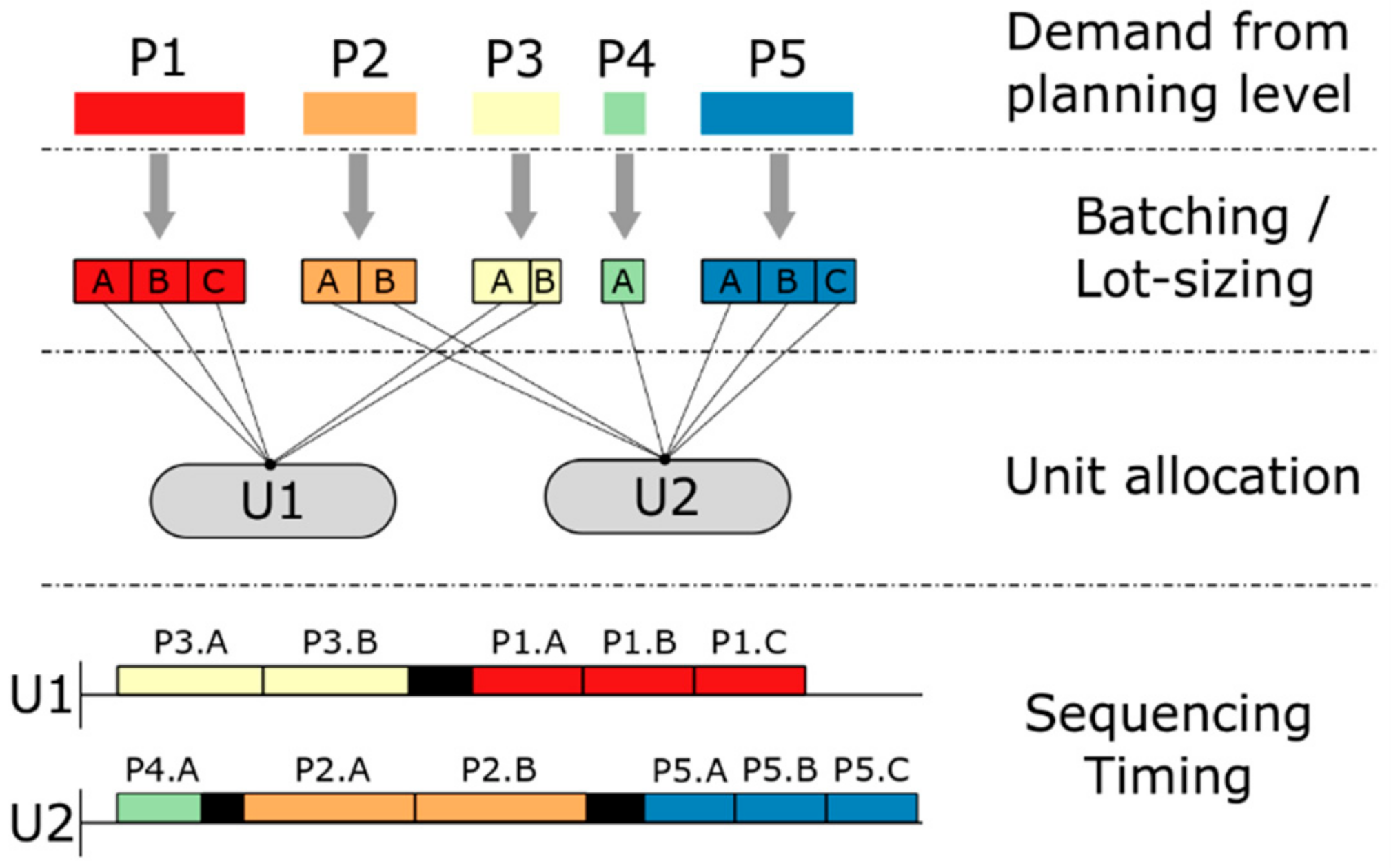
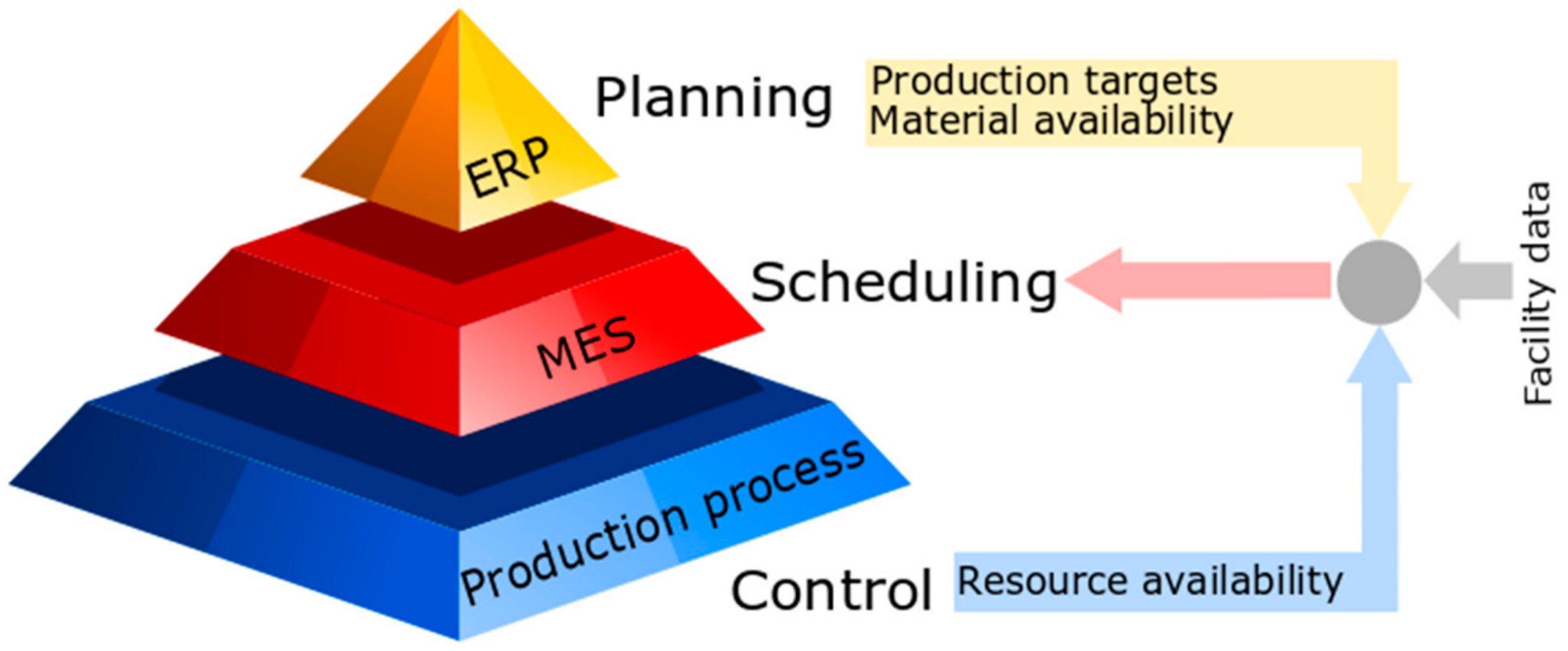
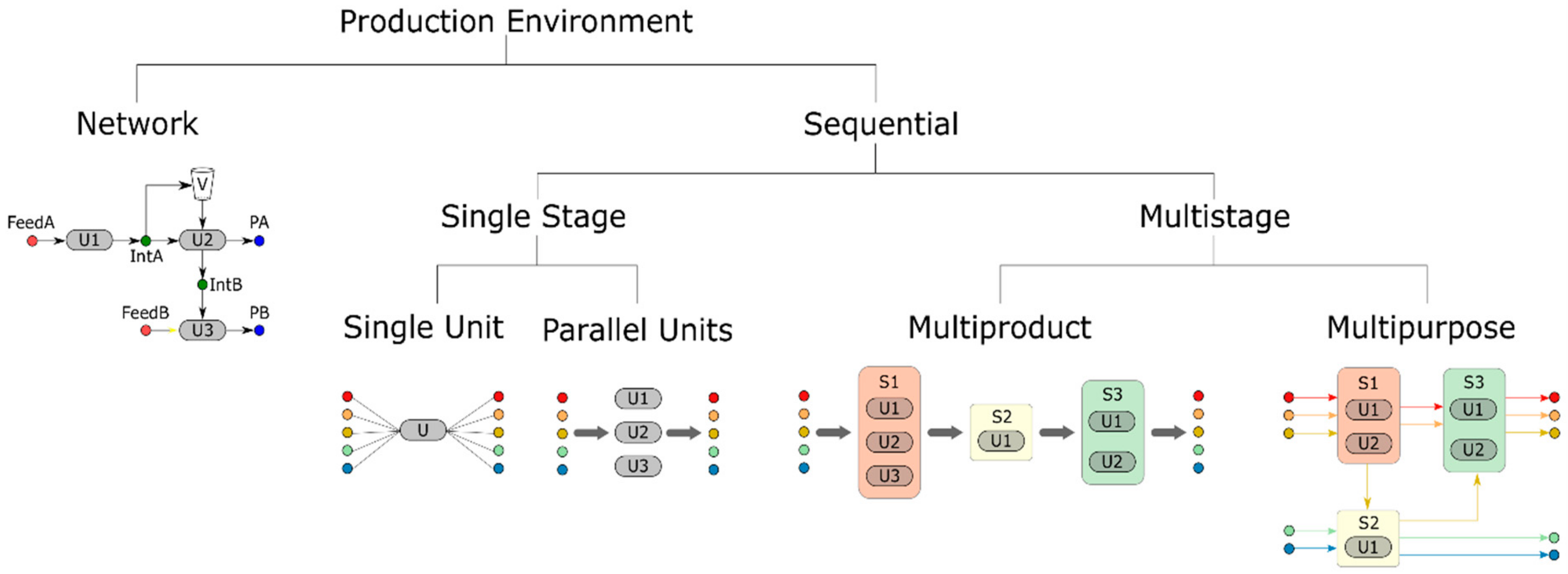
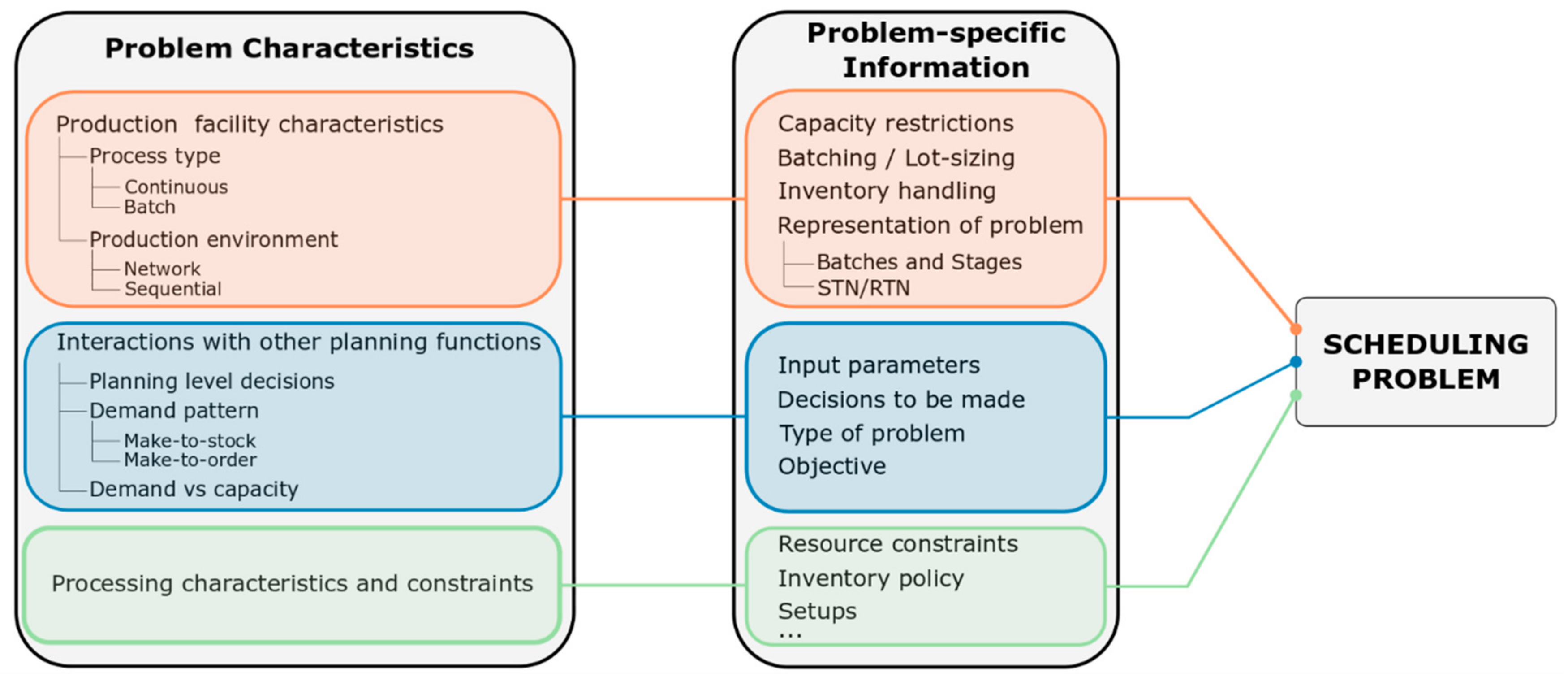
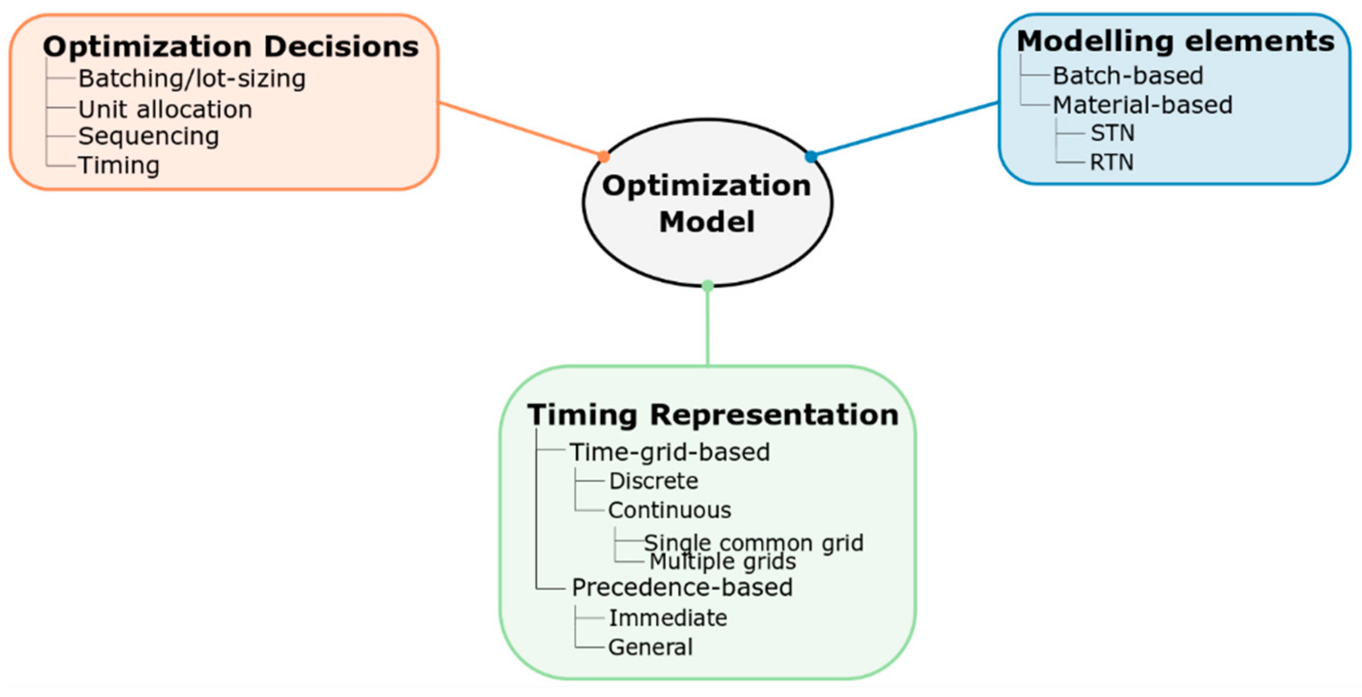
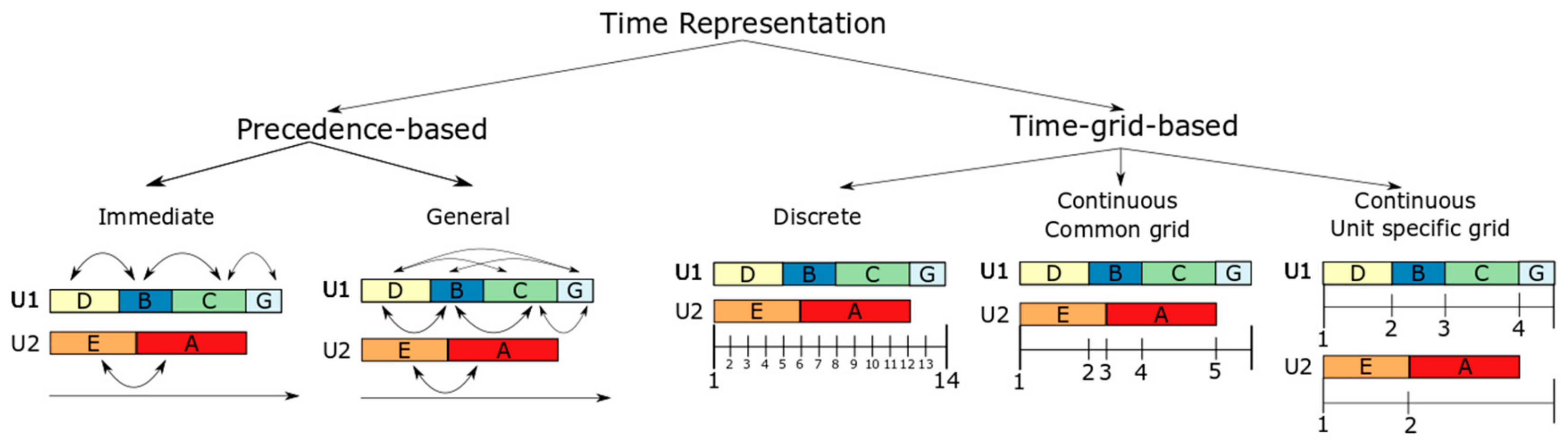
Table 1.
Summary of the industrial applications using optimization-based scheduling approaches.
| Author | Industrial Sector | Main Research Features |
|---|---|---|
| Lin and Floudas [75] | Chemical industry | • Continuous time event-based mixed-integer linear programming (MILP) • Decomposition methodology |
| Janak et al. [129] | Chemical industry | • Graphical user interface development • Rolling horizon approach |
| Westerlund et al. [77] | Chemical industry | • Planning tool connected with the plant’s ERP system |
| Velez, Merchan and Maravelias [78] | Chemical industry | • Multiple discrete-time grids • A real case study from Dow company |
| Moniz et al. [81] | Pharmaceutical industry | • A Visio-based decision-making tool development |
| Stefansson et al. [82] | Pharmaceutical industry | • Discrete and continuous time representations • Stage decomposition |
| Castro, Harjunkoski and Grossmann [83] | Pharmaceutical industry | • Decomposition-based algorithm |
| Kopanos, Méndez and Puigjaner [39] | Pharmaceutical industry | • Precedence-based MILP models • Decomposition-based solution strategy |
| Liu et al. [84] | Pharmaceutical industry | • Maintenance planning • 1 h CPU time |
| Kabra et al. [85] | Pharmaceutical industry | • State-task network (STN) representation • Computational time in the range of 1–2 min. |
| Shah, Sahay and Ierapetritou [86] | Oil refineries | • Six-step MILP based heuristic algorithm • A case study provided by Honeywell Process Solutions (HPS). |
| Zhang and Hua [87] | Oil refineries | • Integration of the plant processes and the utility system |
| Iyer et al. [88] | Oil refineries | • Decomposition algorithm • Feasible solutions within 6600 s are obtained |
| Assis et al. [89] | Oil refineries | • Scheduling of a crude oil terminal • A case study by the national refinery of Uruguay |
| Casrto and Mostafei [90] | Pipeline systems | • A case study from the Iranian Oil Pipelines and Telecommunication Company • 6.2% capacity increase |
| Cafaro et al. [93] | Pipeline systems | • Simultaneous product deliveries are allowed • A case study, related to REPLAN refinery |
| Rejowski and Pinto [94] | Pipeline systems | • Integrality gap of 5.8% in 10,000 CPU s • A case study, related to REPLAN refinery |
| Boschetto et al. [95] | Pipeline systems | • Heuristic rules • Computational times within 3–5 min. |
| Baldo et al. [96] | Food industries | • A novel MILP-based relax and fix heuristic algorithm • A case study from a brewery industry |
| Kopanos, Puigjaner and Maravelias [29] | Food industries | • An immediate precedence-based MILP formulation • A case study from a brewery industry |
| Abakarov andSimpson [97] | Food industries | • A food cannery case study • Scheduling of the sterilization stage |
| Georgiadis et al. [98] | Food industries | • A case study from a large-scale canned fish industry case study • MILP based decomposition algorithm |
| Liu, Pinto and Papageorgiou [99] | Food industries | • An edible-oil deodorized industry case study • Mixed discrete and continuous MILP mathematical |
| Polon et al. [100] | Food industries | • A case study from a sausage production industry • Scheduling of the production stage |
| Doganis and Sarimveis [101] | Dairy industry | • A single yoghurt production line |
| Sel, Bilgen and Bloenhof-Ruwaard [102] | Dairy industry | • Integrated planning and scheduling of a yoghurt facility |
| Touil, Echchatbi and Charkaoui [103] | Dairy industry | • A case study from a milk industry |
| Kopanos, Puigjaner and Georgiadis [104] | Dairy industry | • A case study from a yoghurt industry • Novel resource constraints |
| Georgiadis et al. [105] | Dairy industry | • An integrated software tool connects the plant’s ERP system with the proposed MILP model • A total cost decrease of 20% is achieved |
| Giannelos and Georgiadis [108] | Consumer goods industry | • STN continuous time formulation • Medium-size industrial consumer goods manufacturing process |
| Baumann and Trautmann [110] | Consumer goods industry | • General precedence MILP hybrid method • 10 large-scale problem instances provided by The Procter and Gamble Company |
| Elzakker et al. [106] | Fast-moving consumer goods (FMCG) industry | • A unit-specific, continuous time interval-based algorithm • Ice cream production process of Unilever |
| Kopanos, Puigjaner and Georgiadis [107] | Fast-moving consumer goods (FMCG) industry | • Ice cream production process |
| Elekidis, Corominas and Georgiadis [112] | Consumer goods industry | • An immediate-general precedence-based decomposition algorithm |
| Georgiadis et al. [113] | Manufacturing industries | • Resource task network (RTN) and STN based models • A comparison with a PSE scheduling tool and an MILP model • Development of a middleware interface for data transfer |
| Biondi, Saliba and Harjunkoski [114] | Steel industry | • Slot-based MILP formulation • communication with ERP and DCS |
| Li et al. [116] | Steel industry | • A unit-specific event-based continuous-time MILP model |
| Gajic et al. [117] | Steel industry | • Integrated scheduling and electricity optimization problem • A melt shop case study • 3% electricity cost reduction |
| Hadera et al. [118] | Steel industry | • A melt shop case study • Integrated scheduling and electricity optimization problem • A general precedence MILP scheduling model |
| Castro, Harjunkoski and Grossmann [120] | Steel industry | • Integrated scheduling and energy optimization problem • RTN-based MILP model • 20% electricity cost reduction |
| Wang et al. [122] | glass company | • Bi-objective optimization problem • Makespan and the total energy cost minimization |
| Westerlund, Isaksson and Harjunkoski [123] | Paper Industry | • Trim-loss problem of a paper converting mill |
| Roslöf et al. [124] | Paper Industry | • MILP based decomposition algorithm |
| Giannelos and Georgiadis [126] | Paper Industry | • A slot-based MILP model • A paper mill company case study |
| Castro, Barbosa-Povoa and Matos [127] | Paper Industry | • Continuous and discrete time RTN representation • A case study from a pulp mill plant |
| Castro, Westerlund and Forssell [128] | Paper Industry | • RTN-based formulation • Novel recycling policies |
© 2019 by the authors. Licensee MDPI, Basel, Switzerland. This article is an open access article distributed under the terms and conditions of the Creative Commons Attribution (CC BY) license (http://creativecommons.org/licenses/by/4.0/).
Share and Cite
MDPI and ACS Style
Georgiadis, G.P.; Elekidis, A.P.; Georgiadis, M.C. Optimization-Based Scheduling for the Process Industries: From Theory to Real-Life Industrial Applications. Processes 2019, 7, 438. https://0-doi-org.brum.beds.ac.uk/10.3390/pr7070438
AMA Style
Georgiadis GP, Elekidis AP, Georgiadis MC. Optimization-Based Scheduling for the Process Industries: From Theory to Real-Life Industrial Applications. Processes. 2019; 7(7):438. https://0-doi-org.brum.beds.ac.uk/10.3390/pr7070438
Chicago/Turabian StyleGeorgiadis, Georgios P., Apostolos P. Elekidis, and Michael C. Georgiadis. 2019. "Optimization-Based Scheduling for the Process Industries: From Theory to Real-Life Industrial Applications" Processes 7, no. 7: 438. https://0-doi-org.brum.beds.ac.uk/10.3390/pr7070438
Note that from the first issue of 2016, this journal uses article numbers instead of page numbers. See further details here.