Distributed Model Predictive Control of Steam/Water Loop in Large Scale Ships

Abstract

In modern steam power plants, the ever-increasing complexity requires great reliability and flexibility of the control system. Hence, in this paper, the feasibility of a distributed model predictive control (DiMPC) strategy with an extended prediction self-adaptive control (EPSAC) framework is studied, in which the multiple controllers allow each sub-loop to have its own requirement flexibility. Meanwhile, the model predictive control can guarantee a good performance for the system with constraints. The performance is compared against a decentralized model predictive control (DeMPC) and a centralized model predictive control (CMPC). In order to improve the computing speed, a multiple objective model predictive control (MOMPC) is proposed. For the stability of the control system, the convergence of the DiMPC is discussed. Simulation tests are performed on the five different sub-loops of steam/water loop. The results indicate that the DiMPC may achieve similar performance as CMPC while outperforming the DeMPC method.

1. Introduction

The steam/water loop is an important part of a steam power plant, which plays a role in feed water supply and recycling processes. It is a highly complex and constrained system with multiple variables and interactions [1]. Meanwhile, due to the harsh and challenging operating environment (sea winds, sea waves and sea currents) and various operating modes (automatic start-up, reverse, stop, setting speed, emergency stop and reduction of revolutions) [2], there are difficulties to design a controller that delivers satisfactory performance for the steam/water loop. In order to design an effective approach overcoming the difficulties mentioned above and improving their liability and flexibility of the system, the feasibility of a distributed model predictive control is studied in this paper.

Nowadays, the major concern of the steam power plant is not only the tracking performance, but also other performances such as the consumed energy or safety in terrible conditions. Apart from realizing the load tracking performance, the controllers should also fulfill the flexible requirements for each sub-loop. A general way to improve the flexibility is to apply distributed controllers in the system [3]. Also, the multiple controllers improve the reliability of the system [4]. Concurrently, in order to deal with the constraints in the steam/water loop, model predictive control is selected to maintain good performance for each sub-loop. In fact, such methods are readily matured for various applications in the Industry 4.0 paradigm [5]. For the particular class of complex processes with varying time delays, the simple loop control has been proposed and successfully tested in real life processes [6]. However, the system under investigation in this paper is a multivariable process. Hence, the single loop control does not suffice to guarantee good performance of all sub-system loops.

In recent years, many advanced control strategies have been developed to improve the performance of steam power plants, such as: Advanced PID control [7,8,9,10]; backstepping control [11,12,13]; sliding mode control [14,15,16,17,18]; robust control [19,20]; adaptive disturbance rejection control [21,22,23]. As it has the advantage in dealing with the inputs and outputs constraints, a considerable amount of research has been conducted in the application of model predictive control (MPC) for complex systems in general and for steam power plants, in particular. To overcome the control problems arising from load disturbances and intrinsic nonlinearity, an extended state observer based fuzzy MPC was proposed for the ultra-supercritical boiler-turbine unit [24]. By incorporating both the plant-wide economic process optimization and regulatory process control into a hierarchical control structure, a hierarchical MPC was proposed [25]. A stable fuzzy model predictive controller was designed to solve the superheater steam temperature control problem in a power plant [26], in which the effect of modeling mismatched and unknown plant behavior variations were overcome by the use of a disturbance term and steady-state target calculator. Liu proposed an economic model predictive controller by directly utilizing the economic index of the boiler-turbine system as the cost function. The method realized the economic optimization as well as the dynamic tracking [27].

However, the methods mentioned above are mainly concerned with the loop control of drum steam pressure, electric power and steam–water density in the boiler-turbine system. Most of the concerns concern the tracking performance of the system installed on land. The steam power plant in this paper is installed on ships, and the steam/water loop is depicted in Figure 1 with five sub-loops: Drum water level control loop; deaerator water level control loop; deaerator pressure control loop; exhaust manifold pressure control loop; and condenser water level loop. Also, the steam/water loop in large scale ships has special characteristics compared with those installed on land: (i) Receiving more disturbances from the ocean waves; (ii) smaller capacity; (iii) multiple operation points [28]. Hence, effective control strategies are required to ensure the performance of the steam/water loop.

A linear extended predictive self-adaptive control centralized MPC framework was studied in our previous work. The effects of the predictive horizon and the control horizon on the control system were summarized [28,29]. It was concluded that the predictive horizon be selected according to the system dynamics and the control horizon be selected to ensure a good trade-off between the tracking performance and the computational complexity.

Today’s industry processes, for instance, those in heavy industries (e.g., papermaking, steelmaking, petrochemical and power generation), are becoming more and more complex [30], and are generally composed of a couple of interconnected systems, and possess high nonlinear and stochastic dynamics [31]. Due to the interplay between high performance local control and interactions between subsystem to subsystem, the centralized model predictive control (CMPC) is largely viewed as impractical, inflexible and unsuitable for control of such complex processes [32]. For example, as the authors have five sub-loops in the complete steam/water process, it is necessary to ensure the reliability of the system. This may be achieved by localizing control functions near each sub-loop with remote monitoring and supervision (i.e., distributed control) instead of one central controller (i.e., centralized control). Hence, the applicability of the distributed model predictive control (DiMPC) is investigated in this paper. A comparison is conducted between the decentralized model predictive control (DeMPC), the CMPC and the DiMPC, and the results show the effectiveness of the DiMPC.

The convergence issue is discussed to ensure the stability of the DiMPC. It is proved that the DiMPC, in our study, satisfies certain conditions, under which the properties of the CMPC problem are enjoyed by the DiMPC. Then, by the means provided in [33], the stability of the CMPC is proved, meanwhile, the stability of the DiMPC is guaranteed.

The rest of the paper is organized as follows: Section 2 describes the steam/water loop, and the modeling of the system is shown. The details about the DiMPC, CMPC and DeMPC are introduced in Section 3. Section 4 shows the results and analysis. Finally, some conclusions are drawn in Section 5.

2. Description of the Steam/Water Loop

As shown in Figure 1, the steam/water loop is composed of two main loops, in which one is the water loop indicated by green line and the other is steam loop indicated by red line. The system works as follows. Firstly, the water from the water tank goes to the condenser. Then it is deoxygenated in the deaerator. After being pumped to boiler, the feed water goes into the mud drum due to its high density. The feed water is turned into a mixture of steam and water in the risers. Following this, the steam is separated from the mixture and heated in the superheater. Finally, the steam with a certain pressure and temperature services in the steam turbine. The used steam is sent back to the exhaust manifold and most of the steam is condensed in the condenser, while the remaining part services in the deaerator for deoxygenation [28]. The sub-loops have strong interactions between each other, such as the water level between the deaerator and the condenser, the pressure between the deaerator and the exhaust manifold system. Hence, there are challenges to obtain a desired controller for the steam/water loop.

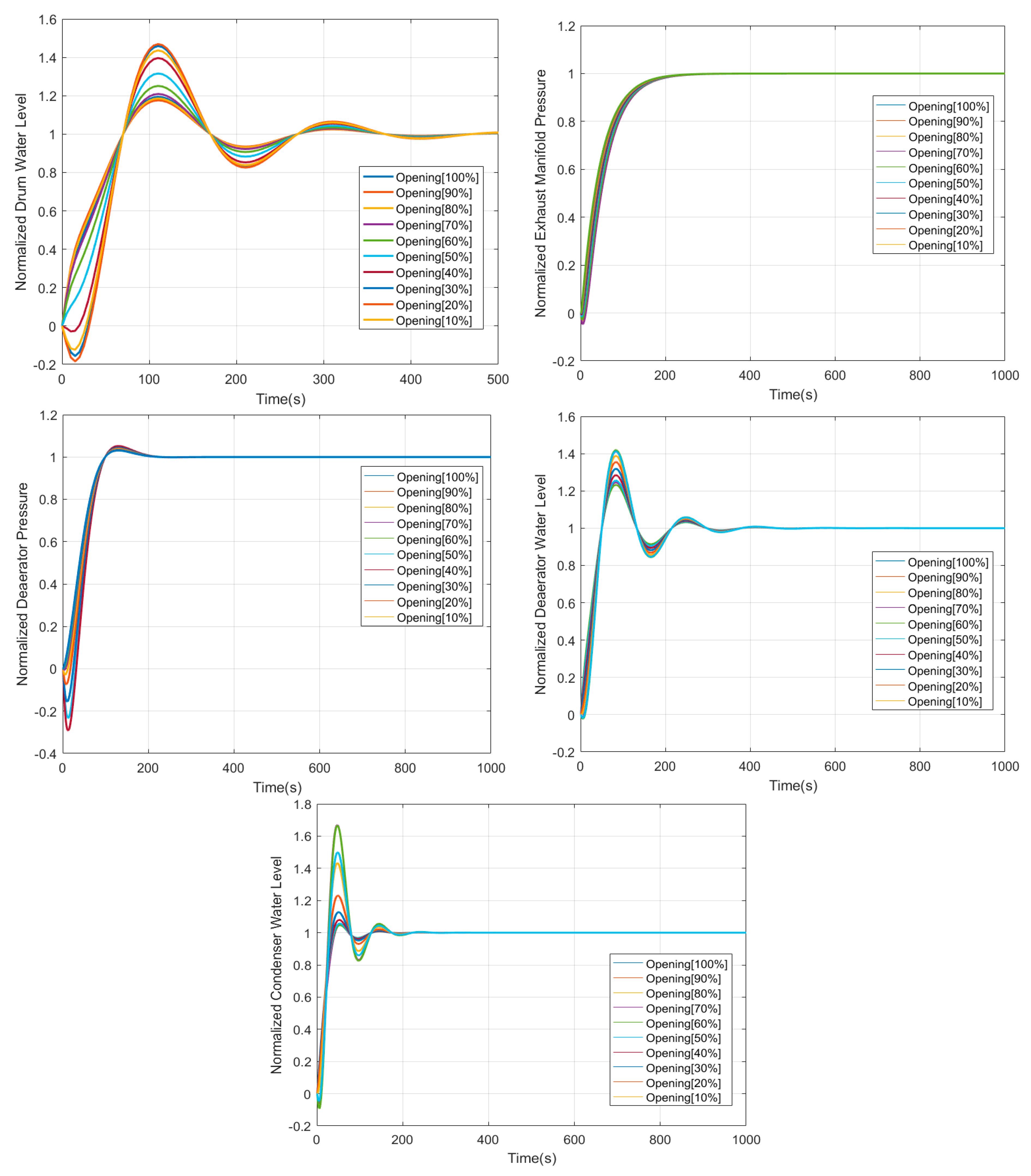
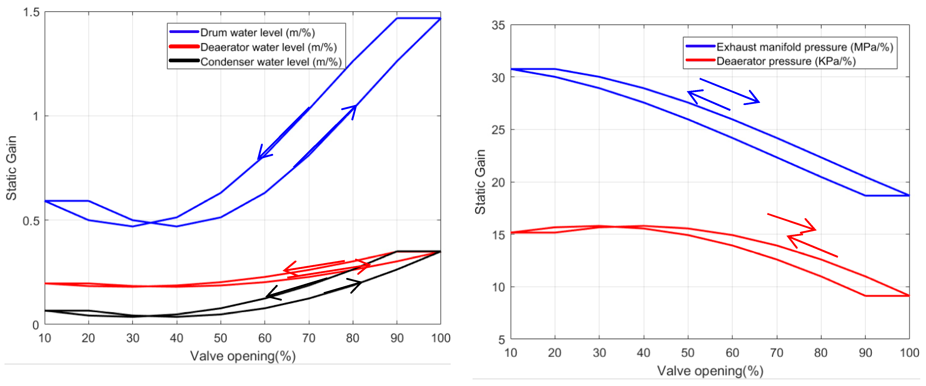
In order to explore the characteristics of the steam/water loop, staircase experiments are conducted around the operating point on the system. The normalized outputs and corresponding static gains are shown in Figure 2; Figure 3, respectively. In the experiment, every 10% step changes are imposed in one input variable, while keeping the other inputs constant. The results show that the static gains change considerably along with the input changes, which indicates the nonlinearity of the system.

By linearization around the operating point, the model of the system is obtained as shown in (1), with five inputs and five outputs. The input vector u = [u₁, u₂, u₃, u₄, u₅] contains the positions of the valves that control the flow rates of feedwater to the drum (u₁), exhaust steam from the exhaust manifold (u₂), exhaust steam to the deaerator (u₃), water from the deaerator (u₄) and water to the condenser (u₅), respectively. The output vector y = [y₁, y₂, y₃, y₄, y₅] contains the values of the water level in drum (y₁), pressure in exhaust manifold (y₂), water level (y₃) and pressure (y₄) in deaerator, and water level of condenser (y₅), respectively. The ranges and operating points of the output variables are listed in

Table 1. The parameters used in the steam/water loop.

Output Variables	Operating Points	Range	Units
Drum water level	1.79	[1.39–2.19]	m
Exhaust manifold pressure	100.03	[87.03–133.8]	MPa
Deaerator pressure	30	[24.9–43.86]	KPa
Deaerator water level	0.7	[0.489–0.882]	m
Condenser water level	0.5	[0.32–0.63]	m

, and the operating points are obtained according to a real large-scale ship.

$$\left[\begin{array}{c}{y}_1\\ \begin{array}{c}{y}_2\\ ⋮\\ y_5\end{array}\end{array}\right]=\left[\begin{array}{cccc}{G}_{11}& G_{12}& \cdots & G_{15}\\ G_{21}& G_{22}& \cdots & G_{25}\\ ⋮& ⋮& \ddots & ⋮\\ G_{51}& G_{52}& \cdots & G_{55}\end{array}\right]\left[\begin{array}{c}{u}_1\\ \begin{array}{c}{u}_2\\ ⋮\end{array}\\ u_5\end{array}\right]$$

(1)

where $G_{11}=\frac{0.0000987}{(s+0.1131)(s+0.0085+0.032j)(s+0.0085-0.032j)}$, $G_{22}=\frac{0.7254}{(s+1.2497)(s+0.0223)}$, $G_{23}=\frac{-0.5}{(s+1.9747)(s+0.0253)}$, $G_{33}=\frac{0.0132}{(s+0.0265+0.0244j)(s+0.0265-0.0244j)}$, $G_{34}=\frac{-0.009}{(s+0.0997)(s+0.0411)}$, $G_{41}=\frac{-0.0008}{(s+0.012+0.126j)(s+0.012-0.126j)}$, $G_{44}=\frac{0.0005152}{(s+0.012+0.038j)(s+0.012-0.038j)}$, $G_{54}=\frac{-0.00015}{(s+0.0175+0.0179j)(s+0.0175-0.0179j)}$, $G_{55}=\frac{0.00147}{(s+0.025+0.0654j)(s+0.025-0.0654j)}$, and other transfer functions $G_{12}=G_{13}=\dots =G_{53}=0$.

The rates and amplitudes of the five inputs are constrained to:

$$\{\begin{array}{ll}-0.007\le \frac{d{u}_1}{dt}\le 0.007& 0\le u_1\le 1\\ -0.01\le \frac{d{u}_2}{dt}\le 0.01& 0\le u_2\le 1\\ -0.01\le \frac{d{u}_3}{dt}\le 0.01& 0\le u_3\le 1\\ -0.007\le \frac{d{u}_4}{dt}\le \mathrm{}0.007& 0\le u_4\le 1\\ -0.007\le \frac{d{u}_5}{dt}\le \mathrm{}0.007& 0\le u_5\le 1\end{array}$$

(2)

The inputs units are normalized percentage values of the valve opening (i.e., 0 represents a fully closed valve, and 1 is completely opened). Additionally, the input rates are measured in percentage per second.

3. Control Strategies

3.1. Introduction for Centralized MPC (CMPC)

The following is a short summary of the extended prediction self-adaptive control (EPSAC) and more details are found in [34]. Consider a discrete system described below:

$$y(k)=x(k)+w(k)$$

(3)

where $k$ is the discrete-time index; $y(k)$ indicates the measured output sequence of system; $x(k)$ is the output sequence of model; and $w(k)$ is the model/process disturbance sequence. The output of the model $x(k)$ depends on the past outputs and inputs, and can be expressed generically as:

$$x(k)=f[x(k-1),x(k-2),\dots ,u(k-1),u(k-2),\dots ]$$

(4)

In EPSAC, the future input consists of two parts:

$$u(k+l|k)=u_{base}(k+l|k)+\delta u(k+l|k)$$

(5)

where $u_{base}(k+l|k)$ indicates lth predicted basic future control scenario and $\delta u(k+l|k)$ indicates the optimizing future control actions, and they are all based on the states and inputs of time k. Then, following the results of lth predicted output is obtained by applying (5) as the control effort.

$$y(k+l|k)=y_{base}(k+l|k)+y_{opt}(k+l|k)$$

(6)

where $y_{base}(k+l|k)$ is the effect of base future control and $y_{opt}(k+l|k)$ is the effect of optimizing future control actions $\delta u(k|k)$, …, $\delta u(k+N_c-1|k)$. The part of $y_{opt}(k+l|k)$ can be expressed as a discrete time convolution as follows:

$$y_{opt}(k+l|k)=h_l\delta u(k|k)+h_{l-1}\delta u(k+1|k)+\dots +g_{l-N_c+1}\delta u(k+N_c-1|k)$$

(7)

where $h_1,\dots h_{N_p}$ are impulse response coefficients; $g_1,\dots g_{N_p}$ are the step response coefficients; N_c, N_p are the control horizon and prediction horizon, respectively. Thus, the following formulation is obtained:

$$Y=\overline{Y}+GU$$

(8)

with, $Y={[y(k+N_1|k)\dots y(k+N_p|k)]}^T$, $U={[\delta u(k|k)\dots \delta u(k+N_c-1|k)]}^T$, $\overline{Y}={[y_{base}(k+N_1|k)\dots y_{base}(k+N_P|k)]}^T$ and

$$G=\left[\begin{array}{cccc}{h}_{N_1}& h_{N_1-1}& \dots & g_{N_1-N_c+1}\\ h_{N_1+1}& h_{N_1}& \dots & \dots \\ \dots & \dots & \dots & \dots \\ h_{N_P}& h_{N_P-1}& \dots & g_{N_P-N_c+1}\end{array}\right]$$

(9)

where N₁ indicates the time-delay in the system.

The disturbance term $w(k)$ is defined as a filtered white noise signal [30]. When there is no information concerning the noise, the disturbance model used in (3) is chosen as an integrator, to ensure zero steady-state error in the reference tracking experiment:

$$w(k)=w(k-1)+e(k)$$

(10)

where e(k) denotes the white noise sequence.

In order to apply EPSAC for a multiple-input and multiple-output (MIMO) system, the individual error of each output is minimized separately. The cost function for the steam/water system with five sub-loops is as follows:

$$J_i={\displaystyle \sum _{l=N_1}^{N_P}{[r_i(k+l|k)-y_i(k+l|k)]}^2}(i=1,2,\dots ,5)$$

(11)

where r_i (i = 1, 2, …, 5) are the setpoints for the five loops.

By defining G_ij as the influence from jth input to ith output, (11) is rewritten as:

$${(R_i-Y_i)}^T(R_i-Y_i)=(R_i-{\overline{Y}}_i-{\displaystyle \sum _{j=1}^5{G}_{ij}{U}_j}{)}^T(R_i-{\overline{Y}}_i-{\displaystyle \sum _{j=1}^5{G}_{ij}{U}_j})$$

(12)

with R_i denotes the reference for loop i, and Y_i denotes the predicted output for loop i.

Taking constraints from inputs and outputs into account, the process to find the minimum cost function becomes an optimization problem which is called quadratic programming.

$$\underset{U_i}{min}{J}_i(U_i)=U_i{}^T{H}_i{U}_i+2f_i{}^T{U}_i+c_i\mathrm{subject}\mathrm{to}AU\le b$$

(13)

$$\mathrm{with}\{\begin{array}{c}{H}_i=G_{ii}^T{G}_{ii}\hspace{1em}{f}_i=-G_{ii}^T(R_i-{\overline{Y}}_i-{\displaystyle \sum _{j=1,j\ne i}^5{G}_{ij}{U}_j)}\\ c_i=(R_i-{\overline{Y}}_i-{\displaystyle \sum _{j=1,j\ne i}^5{G}_{ij}{U}_j{)}^T(R_i-{\overline{Y}}_i-{\displaystyle \sum _{j=1,j\ne i}^5{G}_{ij}{U}_j)}}\end{array}$$

where A is a matrix; b is a vector according to the constraints and U_i is the input for sub-loop i.

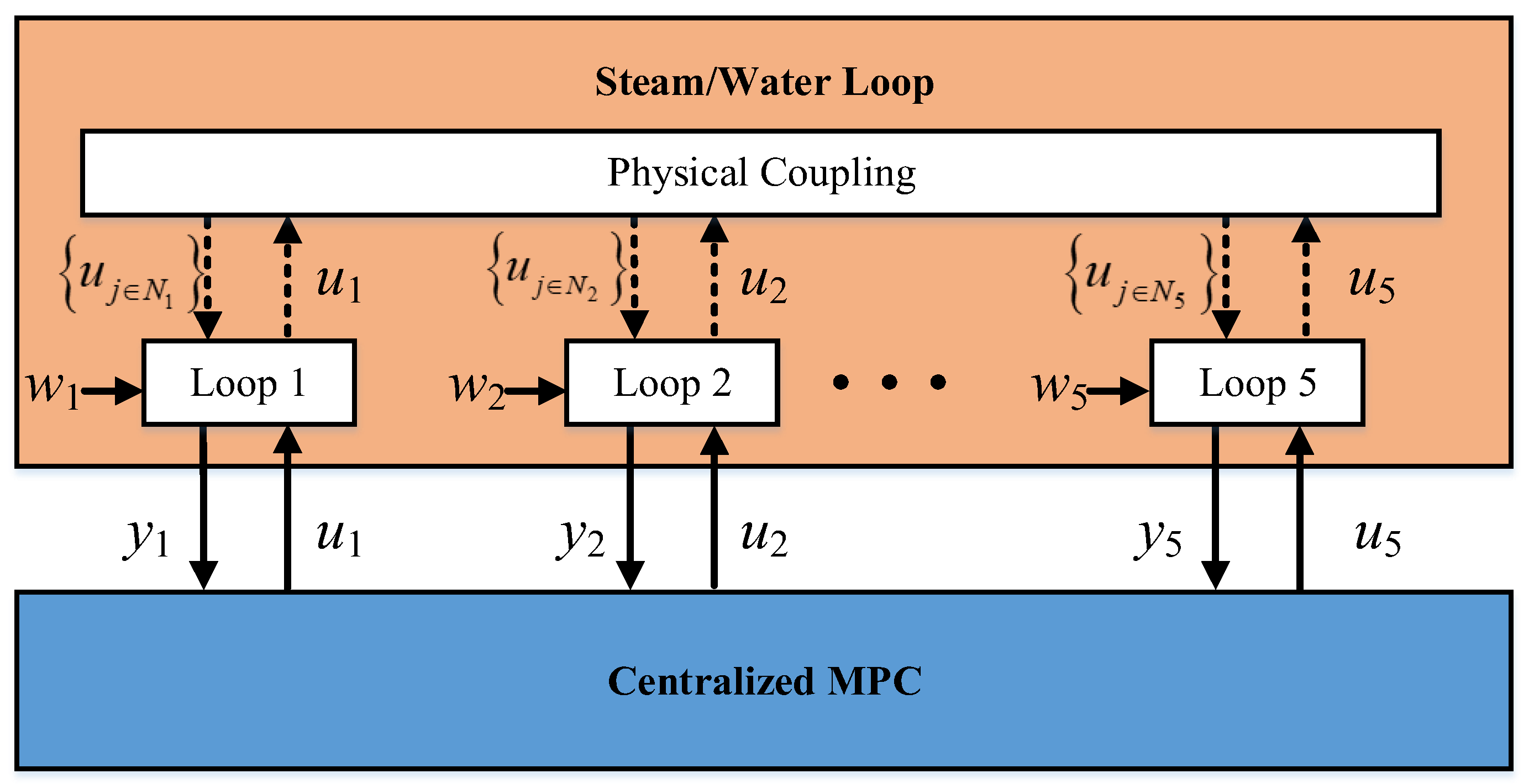
Figure 4 shows the conceptual representation of the centralized MPC [35]. To get the optimal solutions for sub-loop i, the interaction $\left\{u_{j\in N_i}\right\}$, $N_i=\left\{j\in N:{\tilde{G}}_{ij}\ne 0\right\}$ from other sub-loops is taken into account as shown in (13).

Hence, the optimal centralized solution U = [U₁ U₂ U₃ U₄ U₅] is obtained by solving the following global cost function:

$$J={\displaystyle \sum _{i=1}^5{p}_i{J}_i}$$

(14)

where $J_i$ are defined in (11), and $p_i$ are weighting factors. In our case, the $p_i$ are chosen as the values which can normalize the cost function $J_i$.

3.2. Proposed Distributed MPC (DiMPC)

It is noteworthy to mention that the centralized approach implies that all the information regarding to all the sub-systems (or sub-loops) is gathered in a single controller, as showed in Figure 4. The advantage is straightforward since the cost function (14) has an optimal solution. However, if one sub-loop malfunctions, then the entire steam/water loop collapses, with serious consequences for safety of the large scale ship.

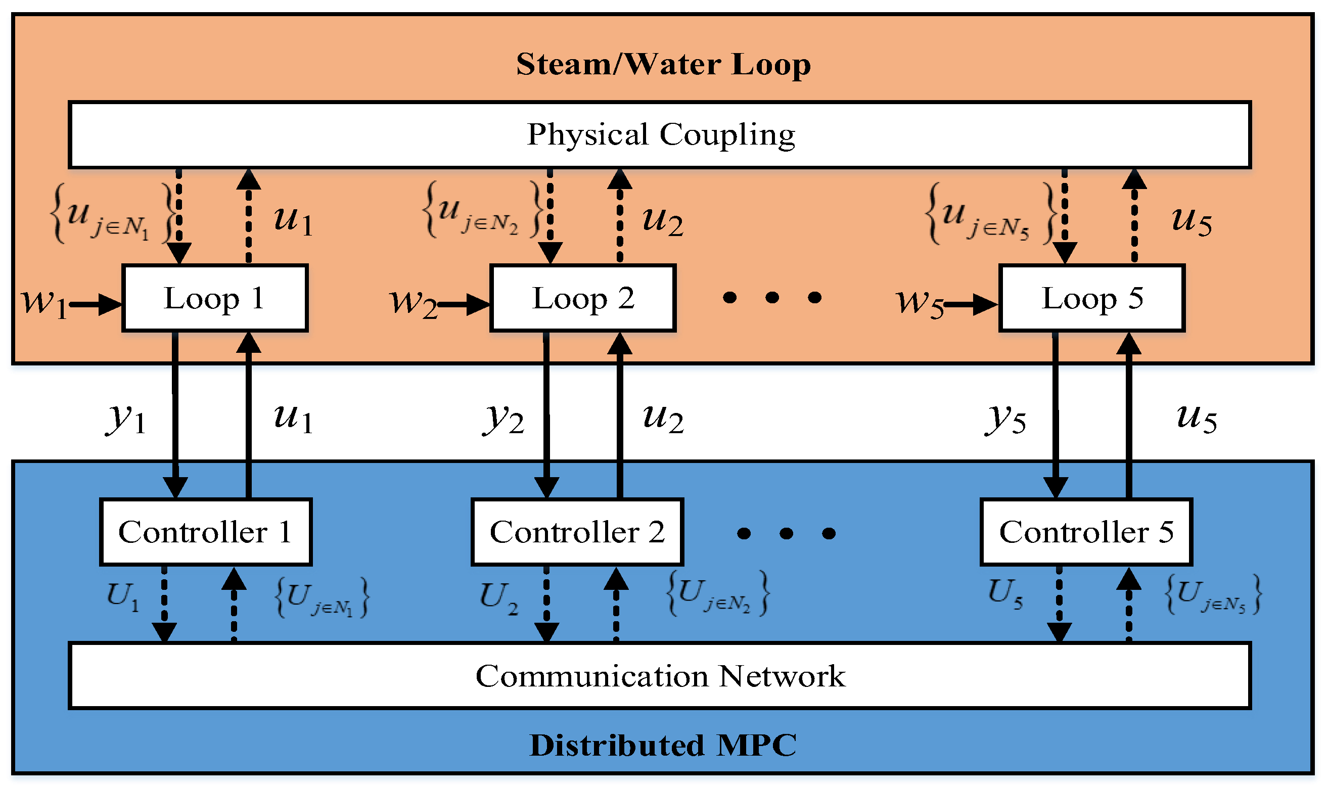
One solution is provided by the distributed MPC (DiMPC) method, that regards all the sub-systems as independent modules which are controlled by an individual controller. Through the communication network, the inherent interactions are considered.

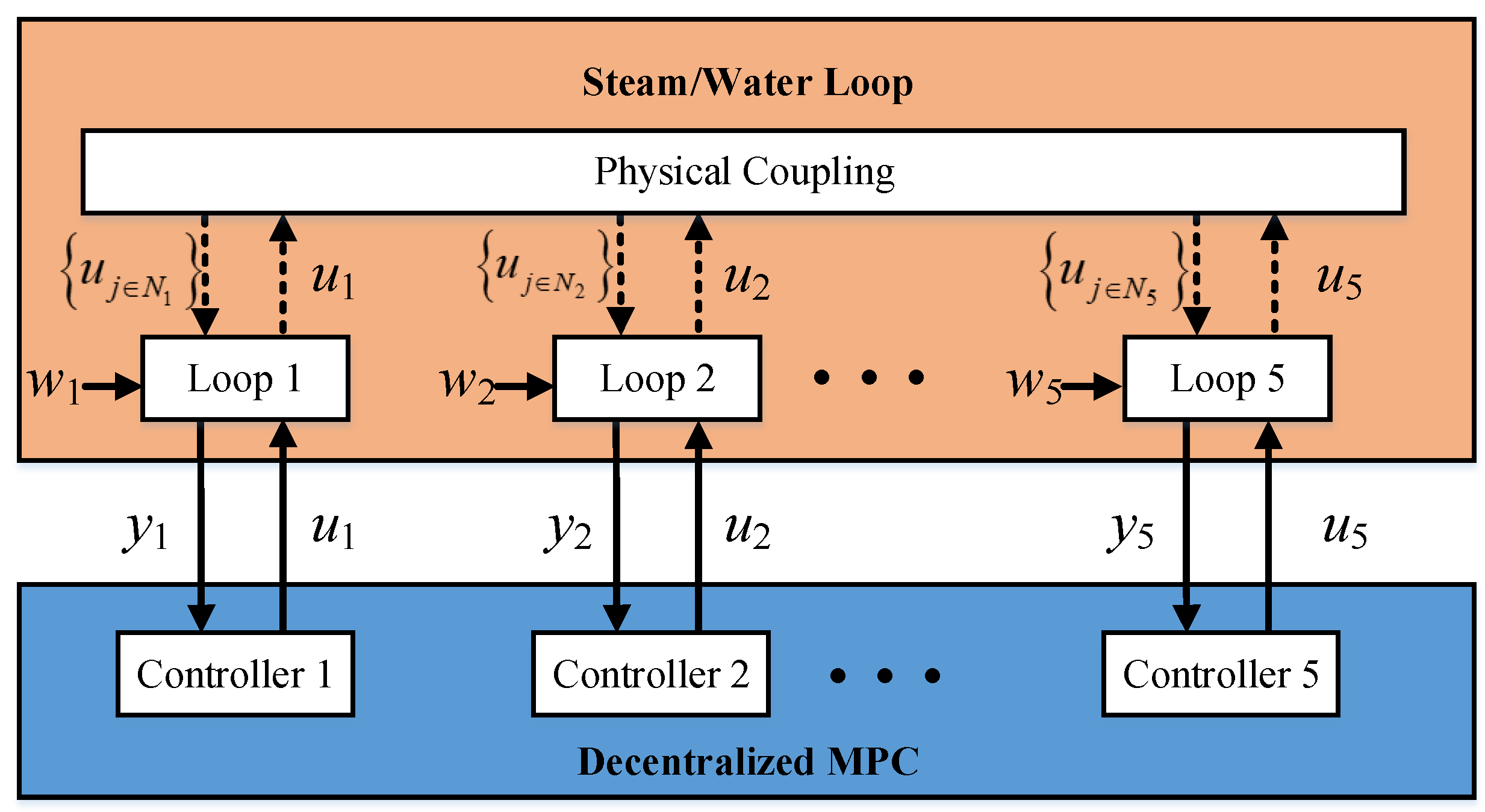
Thus, the same local cost function (13) is locally minimized by each controller, in which the coupling term ${\displaystyle \sum _{j=1,j\ne i}^5{G}_{ij}{U}_j}$ is computed with the input trajectory $U_j$ received from the neighbors, and several iterations are performed until the local optimal solution is reached. For the sake of clarity, conceptual representation of the distributed MPC architecture is shown in Figure 5, and a pseudo-code is provided:

Algorithm 1 The Iterative DiMPC

Step 1: Sub-loop I receives an optimal local control action $\delta U_i$ at the iterative time as iter = 0 according to the EPSAC, and the local control action $\delta U_i$ can be rewritten as $\delta U_i^{iter}$, where $\delta U_i$ indicates the vector of the optimizing future control actions with length of Nci; Step 2: The $\delta U_j^{iter}$ ($j\in N_i$) is communicated to the loop i, and the $\delta U_i^{iter+1}$ is calculated again with the $\delta U_j^{iter}$ from other loops; Step 3: If the termination conditions $\Vert \delta U_i^{iter+1}-\delta U_i^{iter}\Vert \le {\epsilon }_i\vee iter+1>\overline{iter}$ are reached, the $U_i^{iter+1}$ is adopted, where ${\epsilon }_i$ is the positive value and $\overline{iter}$ indicates the upper bound of the number of iteration times. Otherwise, the iter is set as iter = iter + 1, and return to Step 2; Step 4: Calculate the optimal control effort as $U_t=U_{base}+\delta U^{iter}$, and the control effort is applied to the system; Step 5: Set t = t + 1, return to Step 1.

3.3. Classical Decentralized MPC (DeMPC)

In Figure 6, the conceptual representation of the DeMPC is presented. When comparing with the distributed strategy from Figure 5, it can be seen that the main difference is given by the fact that the controllers do not exchange information, although the physical coupling remains.

Hence, the local cost function to be minimized by each controller is:

$$\underset{U_i}{min}{J}_i(U_i)=U_i{}^T{H}_i{U}_i+2f_i{}^T{U}_i+c_i\mathrm{subject}\mathrm{to}AU\le b$$

(15)

$$\mathrm{with}\{\begin{array}{c}{H}_i=G_{ii}^T{G}_{ii}\hspace{1em}{f}_i=-G_{ii}^T(R_i-{\overline{Y}}_i)\\ c_i={(R_i-{\overline{Y}}_i)}^T(R_i-{\overline{Y}}_i)\end{array}$$

which is derived from (13), by removing the coupling influence between sub-loops.

3.4. Multiple Objective Distributed Model Predictive Control (MODiMPC)

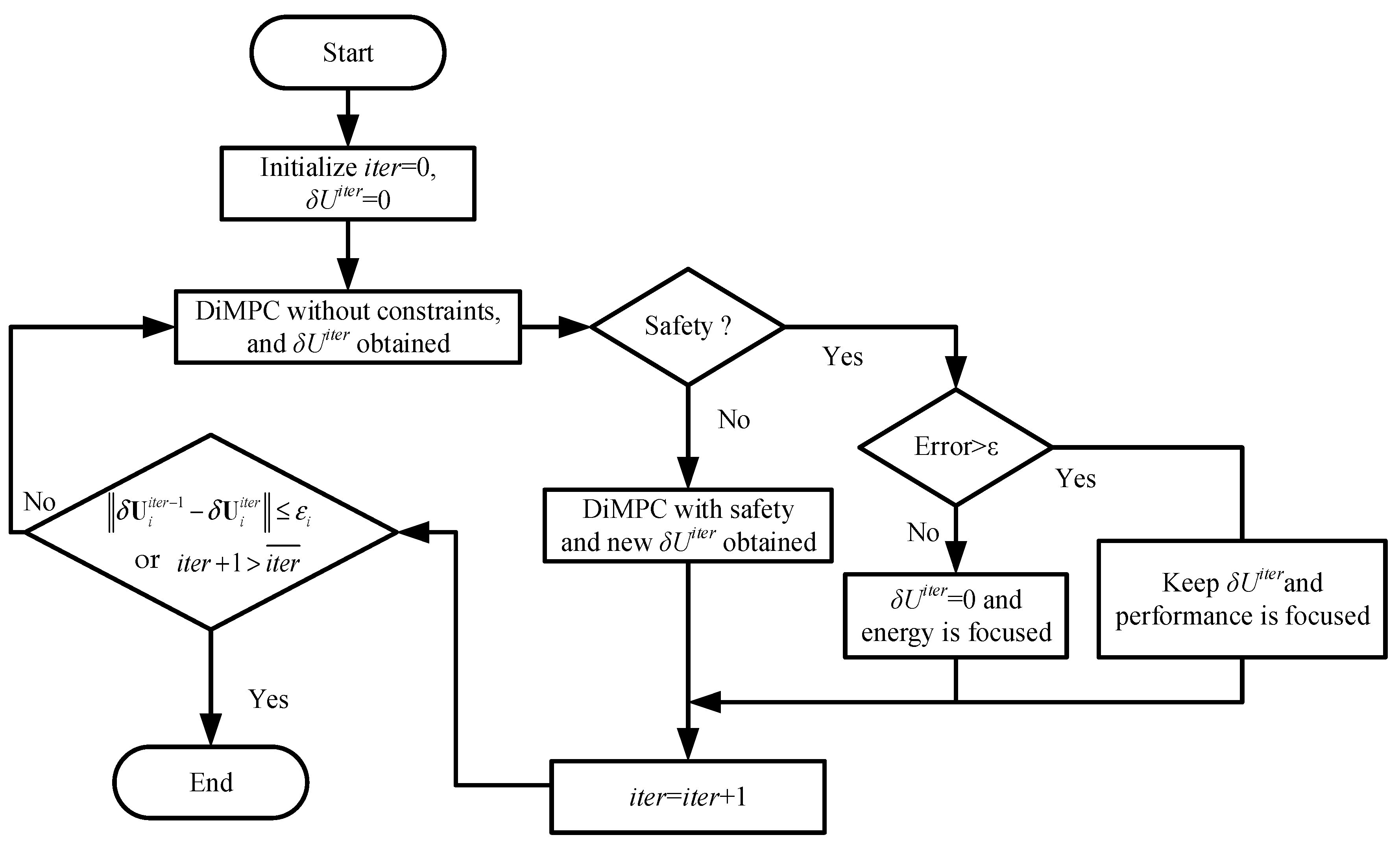
Nowadays, setpoint tracking is not the only target for the control system. For some fast dynamic systems, the computing speed of the control strategies has an important influence. In order to improve the computing speed, a small loss in tracking performance is made to realize the fast computing speed. The scheme of the MODiMPC is shown in Figure 7. There are three layers of structure, in which the priority is shown as safety > tracking performance > energy.

The algorithm starts from initial zero conditions and computes the optimal control effort as an unconstrained solution of the optimization problem that aims to minimize the tracking error.

If the predicted inputs or outputs are not safe (generally out of the hard constraints), the constraints is included in the optimization to ensure safety. If the variables are in the safety interval, then according to the tracking error condition, two options are available, namely: (i) Error > ε, the focus is on performance, and the control effort is kept $\delta U_i^{iter}$, (i.e., the control effort is kept to the one which minimizes the cost function with (11)); or (ii) Error < ε, the focus is on energy, and the control effort is kept $\delta U_i^{iter}=0$ (i.e., the actuator does not need to do any change), where ε is a tolerance error, and in this paper, it is chosen as 1% of the upper bound of the corresponding output. According to the end conditions ($\Vert \delta U_i^{iter+1}-\delta U_i^{iter}\Vert \le {\epsilon }_i\vee iter+1>\overline{iter}$) of the DiMPC, the procedure stops or continues to obtain a new result.

Due to the hydraulic cylinder being linked with the valve in the steam/water loop, the frequent changes in valves mean frequent changes in the hydraulic cylinder, which results in a large energy costs. In this sense, the energy is saved if the valves do not need to do any change under the condition Error < ε.

In the traditional MPC, the influence from constraints has always been considered to obtain the optimal inputs for the system. In our study, the quadratic programming is applied. However, the setpoint does not always change during the operation of the system, and most of the time, the system operates at a stable operating point. During this kind of period, the only thing to be considered is energy, in which the control effort is always kept the same as the last sampling time. Hence, no optimization process exists anymore, and there is a huge reduction in computing time.

3.5. Convergence Issue

In order to analyze the stability of the optimal solution of the distributed control system, first the convergence issue is discussed. A standard MPC formulation is written in a form of a series of static optimization problems shown as follows:

$$S{P}_k:\underset{S}{\min }J(S)$$

(16)

$$\begin{array}{r}\mathrm{s}.\mathrm{t}.M(S)=0\\ C(S)\le 0\end{array}$$

where S is the vector of the decision variables, including the state variables X and the control variables U. M(S) is the prediction model and C(S) denotes the constraints. Although our process model has an input-output formulation, it can be easily translated into a state-space definition.

In the DiMPC, Equation (16) is decompositioned into subproblems. For the sub-loop i:

$$S{P}_{ki}:\underset{S_i}{\min }{J}_i(S_i,S_i^{nei})$$

(17)

$$\begin{array}{r}\mathrm{s}.\mathrm{t}.M_i(S_i,S_i^{nei})=0\\ C_i(S_i,S_i^{nei})\le 0\end{array}$$

where S_i is the vector of the decision variables for sub-loop i, and $S_i^{nei}$ is the vector of the variables for the sub-loops that have interaction with sub-loop i. M_i and C_i meet the conditions: ${\displaystyle {\cup }_i{S}_i}=S,{\displaystyle {\cup }_i{M}_i}=M,{\displaystyle {\cup }_i{C}_i}=C$.

According to [35], if the distributed control methodologies satisfy some conditions, the properties that can be proved for the equivalent CMPC problem are enjoyed by the solution obtained using the DiMPC implementation. Also, the convergence issue of the DiMPC is equal to the CMPC. The optimal results from the DiMPC converge to the global optimal point. The conditions are listed as follows:

(1)

The sub-loops can completely cover the full large system;

(2)

J_i and C_i are convex;

(3)

The sub-loops work sequentially;

(4)

The starting point is in the interior of the feasible region;

(5)

Each sub-loop cooperates with its neighbors in that it broadcasts its latest iteration to these neighbors;

(6)

Each sub-loop uses the same optimal method to generate its iterations.

However, the conditions 2 and 3 are over strict as many systems are nonconvex and have nonlinearity in reality. Further, [36,37] show that these two conditions can be relaxed to nonconvex optimal problems with nonlinearity.

Moreover, the convergence of the DiMPC is further analyzed using the study given in [33]. Hence, starting from the unconstrained optimal solution of the distributed algorithm, the idea is to rewrite it with a recursive matrix formulation. After some matrix manipulation, a compact description is obtained:

$${\mathrm{U}}^{*}(k)=\mathrm{F}(k)-{\hat{\mathrm{H}}\mathrm{U}}^{*}(k-1)$$

(18)

where ${\mathrm{U}}^{*}\left(k\right)$ consists of the optimal sequences of all the sub-loops, computed at sample time k, while ${\mathrm{U}}^{*}(k-1)$ are the shifted optimal trajectories computed at the previous sampling time k − 1, with the last term doubled, to ensure the dimensions consistencies. The term $\mathrm{F}(k)$ is variable and computed at each sampling instant using the prediction error, whereas $\hat{\mathrm{H}}$ is a constant term that is computed off-line in the initialization stage of the algorithm (see [33] for further details).

Note that using Equation (18), the convergence of the local optimal solutions can be checked by verifying that all the eigenvalues from $\hat{\mathrm{H}}$ are inside the unit circle. Additionally, Equation (18) can be reformulated in the classical system approach as:

$${\mathrm{U}}^{*}(k)=(\mathrm{I}-q^{-1}\hat{\mathrm{H}})\mathrm{F}(k)$$

(19)

where $q^{-1}$ is an operator that shifts the data backward one sampling period, $\mathrm{F}(k)$ is regarded as the system’s input, while ${\mathrm{U}}^{*}\left(k\right)$ denotes the system’s output. It is noteworthy to mention that Equation (19) can be used to analyze the stability of the optimal solution ${\mathrm{U}}^{*}\left(k\right)$ at sampling time k, in the classical linear time-invariant framework by verifying that all the eigenvalues of the system equivalent matrix $(\mathrm{I}-q^{-1}\hat{\mathrm{H}})$ are inside the unit circle. Furthermore, if this condition is satisfied on the equality case, it results in the optimal solution of the distributed algorithm being marginally stable.

Hence, using this simple approach, the evolution of the system is computed using $\mathrm{F}(k)$ as the system’s input, which is calculated using the prediction error from each sampling period. Although this is an analytical approach to recursively place the system’s progression in time, it can be straightforwardly computed in an automatic manner, using the simulation tools available for a control engineer. Moreover, all the computations are computed in a distributed manner, since using Equation (18), each sub-loop computes the optimal trajectories of the coupling neighbors, and knowing this information, it computes its own optimal trajectory at each sampling instant.

4. Simulation Results and Analysis

According to our previous work, the parameter configuration for the EPSAC method is shown in

Table 2. The parameters applied in various MPC controllers.

Controllers	Nc	Ts	Np	N1	Ns
DeMPC CMPC DiMPC	Nc1 = 4, Nc2 = 1, Nc3 = 1, Nc4 = 4, Nc5 = 6 samples	5 s	Np1 = 20; Np2 = 15; Np3 = 15; Np4 = 20; Np5 = 20 samples	1	300

.

Where the T_s is the sampling time; N_c1, N_c2, …, N_c5 are control horizons; (the control horizons were selected by finding a good trade-off between tracking performance and computation time for each loop), N_p1, N_p2, …, N_p5 are prediction horizons of the five loops, respectively (the prediction horizons were selected taking into account the specific transient dynamics for each loop); N_s is the number of the samples. The step setpoints are provided in

Table 3. Step setpoints changes in the experiments.

Time (s)	2–300	300–600	600–900	900–1200	1200–1500
Drum Water Level (m)	2	2	2	2	2
Exhaust Manifold Pressure(MPa)	100.03	116	116	116	116
Deaerator Pressure (KPa)	30	30	35	35	35
Deaerator Water Level(m)	0.7	0.7	0.7	0.8	0.8
Condenser Water Level(m)	0.5	0.5	0.5	0.5	0.6

. In the experiments, the initial condition was set at the operating point of the steam/water loop.

The simulation results are shown in Figure 8, including the system outputs and the corresponding control efforts. In order to test which case provides the best result, performance indexes in an average value for the five sub-loops were compared including integrated absolute relative error (IARE), integral secondary control output (ISU), ratio of integrated absolute relative error (RIARE), ratio of integral secondary control output (RISU) and combined index (J). These indexes are calculated with the following expressions:

$$IARE=\frac{1}{5}{\displaystyle \sum _{i=1}^5{\displaystyle \sum _{k=0}^{N_s-1}\left|r_i(k)-y_i(k)\right|/r_i(k)}}$$

(20)

$$ISU=\frac{1}{5}{\displaystyle \sum _{i=1}^5{\displaystyle \sum _{k=0}^{N_s-1}{(u_i(k)-u_{ss}{}_i(k))}^2}}$$

(21)

$$RIARE(C_2,C_1)=\frac{IARE(C_2)}{IARE(C_1)}$$

(22)

$$RISU(C_2,C_1)=\frac{ISU(C_2)}{ISU(C_1)}$$

(23)

$$J(C_2,C_1)=\frac{w_{1}RIARE(C_2,C_1)+w_{2}RISU(C_2,C_1)}{w_1+w_2}$$

(24)

where $u_{ssi}$ is the steady state value of the ith input; C₁, C₂ are the compared controllers and the weighting factors w₁ and w₂ in (24) are chosen as w₁ = w₂ = 0.5.

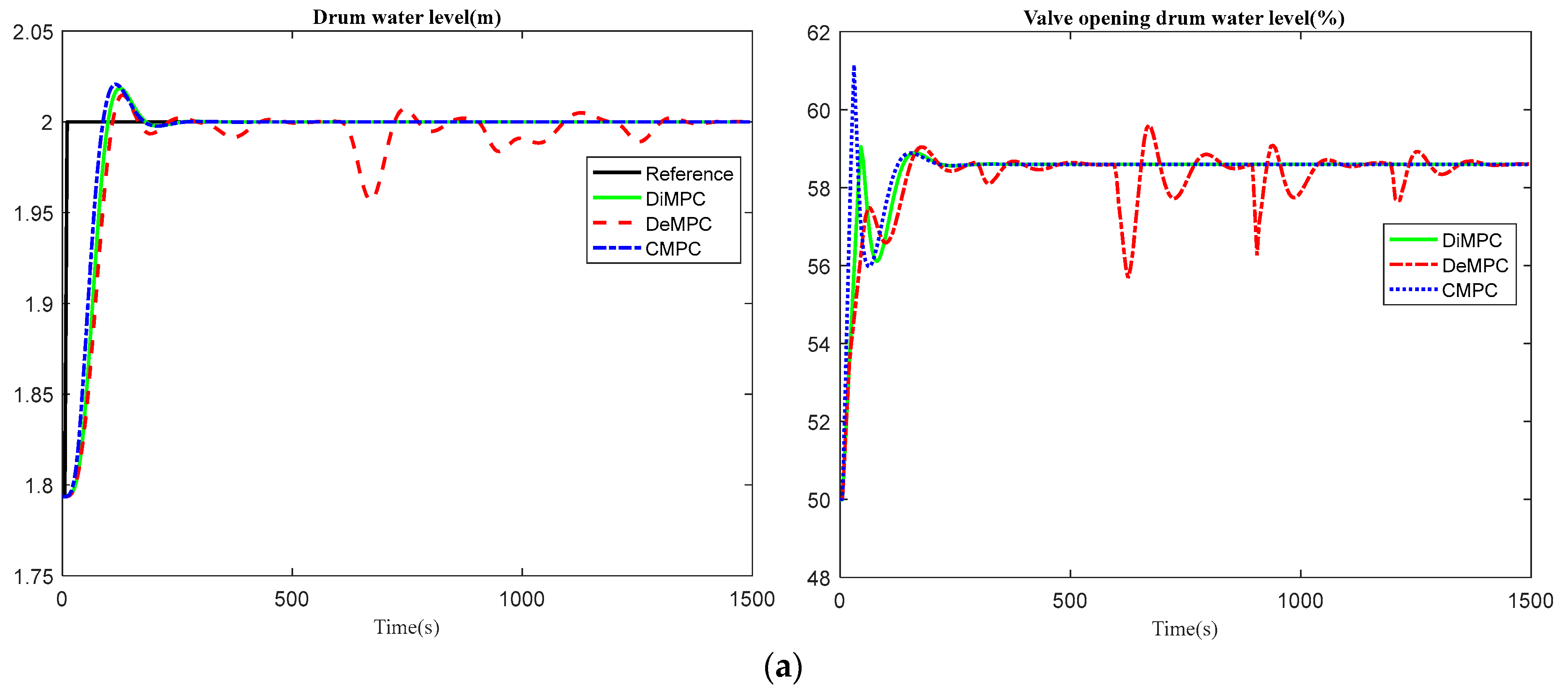
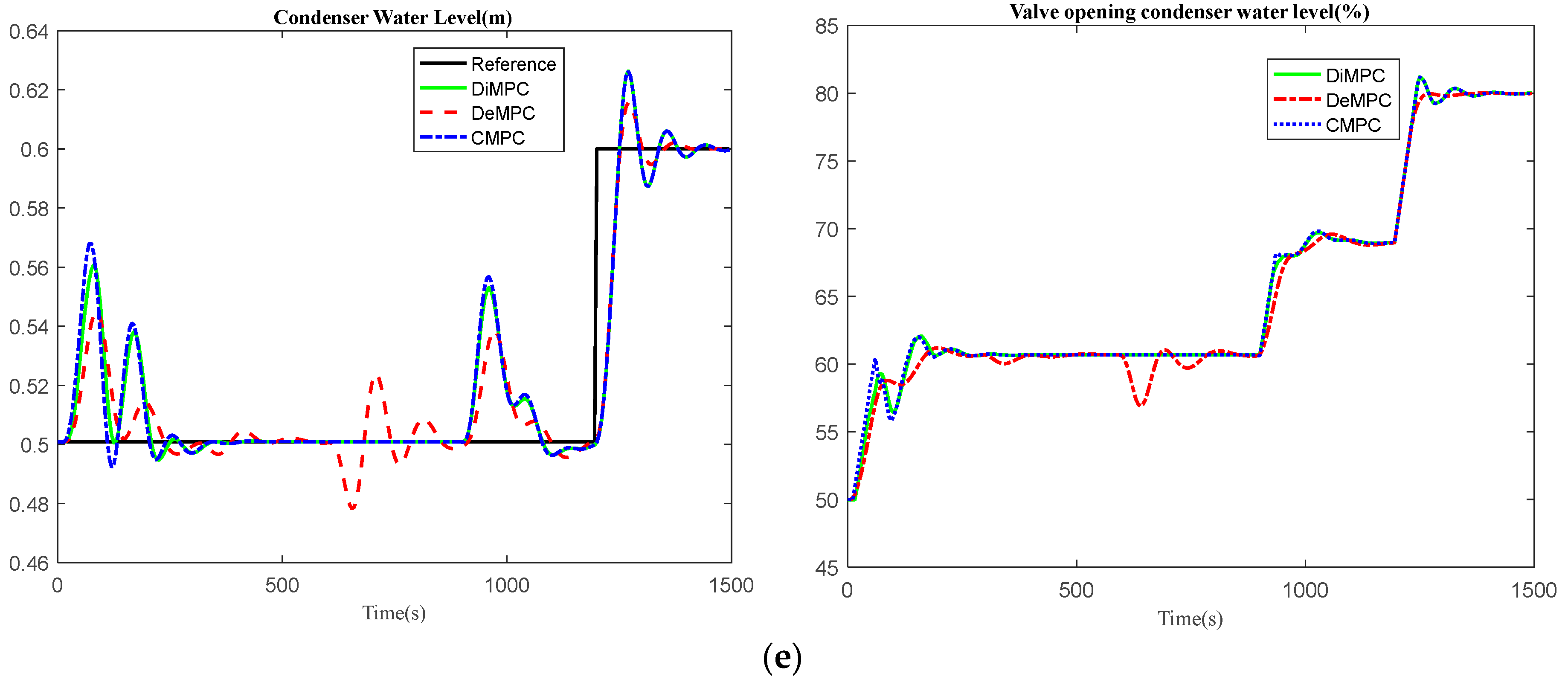
As depicted in Figure 8, the CMPC had similar performance as the DiMPC, and both outperformed the DeMPC. This conclusion is not only valid for this process, but also for other processes, since the DeMPC strategy does not take the interactions into account, which lead to some severe fluctuations when the setpoint changes in other variables. Although the control efforts in the DiMPC are obtained separately, the performance is still good due to the iteratively communication between the controllers for each sub-loop. In real life operations, where the addition of the effects of noise and stochastic disturbances are needed, perhaps with adding periodic disturbances from sea dynamics, the DeMPC may even lead to instability in the overall system.

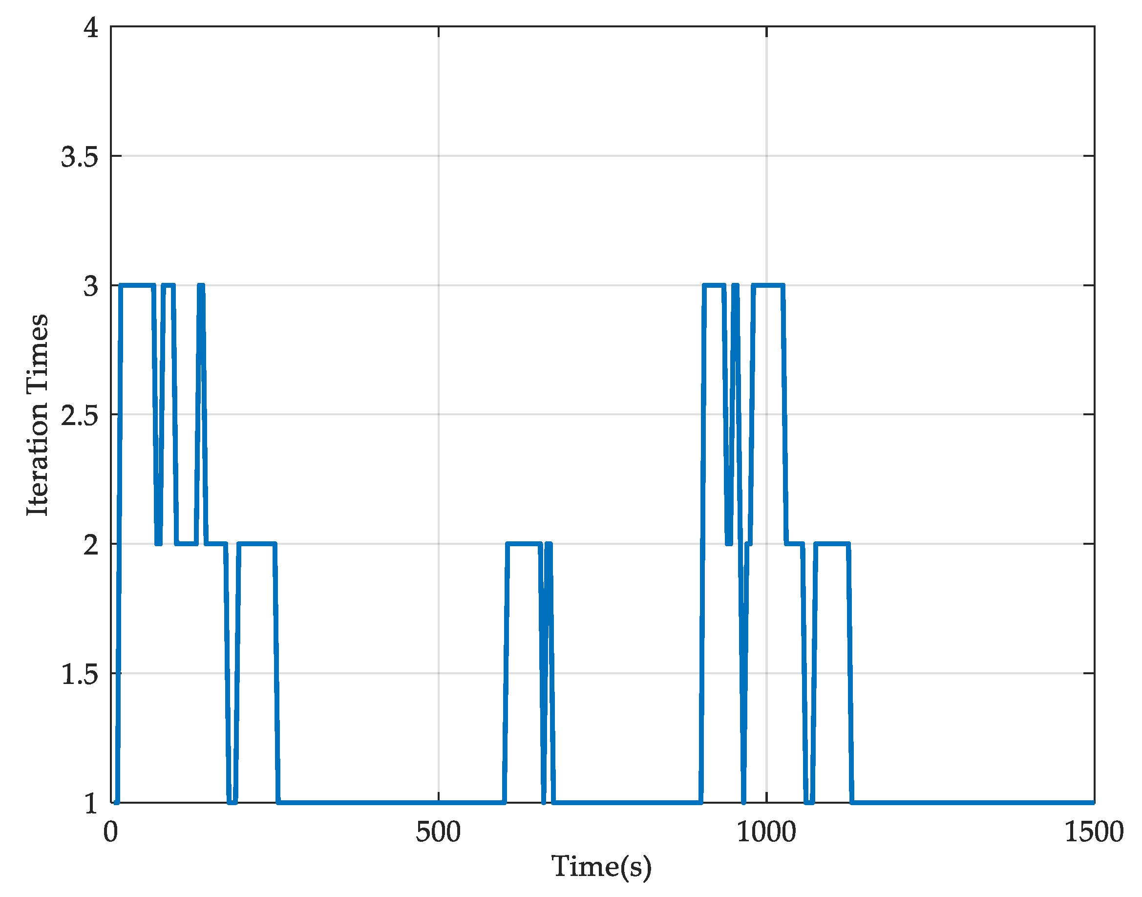
The iterations are shown in Figure 9 during the optimization of DiMPC. In the algorithm, the two conditions to end the iteration are designed as: (i) The difference between consecutive optimal inputs fulfill the condition $\Vert \delta U_i^{iter+1}-\delta U_i^{iter}\Vert \le 0.002$ ; (ii) the maximum iteration time is five, i.e., $iter>5$.

The same conclusion is also obtained according to the numerical values shown in

Table 4. Performance indexes for IARE and ISU.

Index	DiMPC	DeMPC	CMPC
IARE	2.5117	2.7507	2.4795
ISU	0.4672	0.4686	0.4937

;

Table 5. Performance indexes for RIARE and RISU.

Index	DiMPC VS DeMPC	DeMPC VS CMPC	CMPC VS DiMPC
RIARE	0.8959	1.1417	1.0011
RISU	0.8863	1.1629	1.0290
J	0.8911	1.1523	1.0151

. As the index J implies, the DiMPC and CMPC have similar results. However, there is only one controller in the CMPC, which means the system may be out of service if there is any problem with the controller. On the contrary, the DiMPC has more ability in fault-tolerance and flexibility without much performance loss compared with the CMPC. As the DiMPC only needs a part of the entire model, it is much easier to find a feasible solution, while CMPC needs the entire model to obtain all the solutions at one time. In this context, the DiMPC has better robust performance than the CMPC. Hence, the system model required for the DiMPC can be less accurate than the CMPC. In an industry context, a staggering 60–70% of the project time is spent on model development, while the rest is claimed for the controller design and validation [38]. Hence, any reduction in identification time requirement greatly diminishes overall loop maintenance control related costs. The analysis given in this paper provides a trade-off solution, yet with acceptable performance but with great yields for cost reduction in control design and validation time.

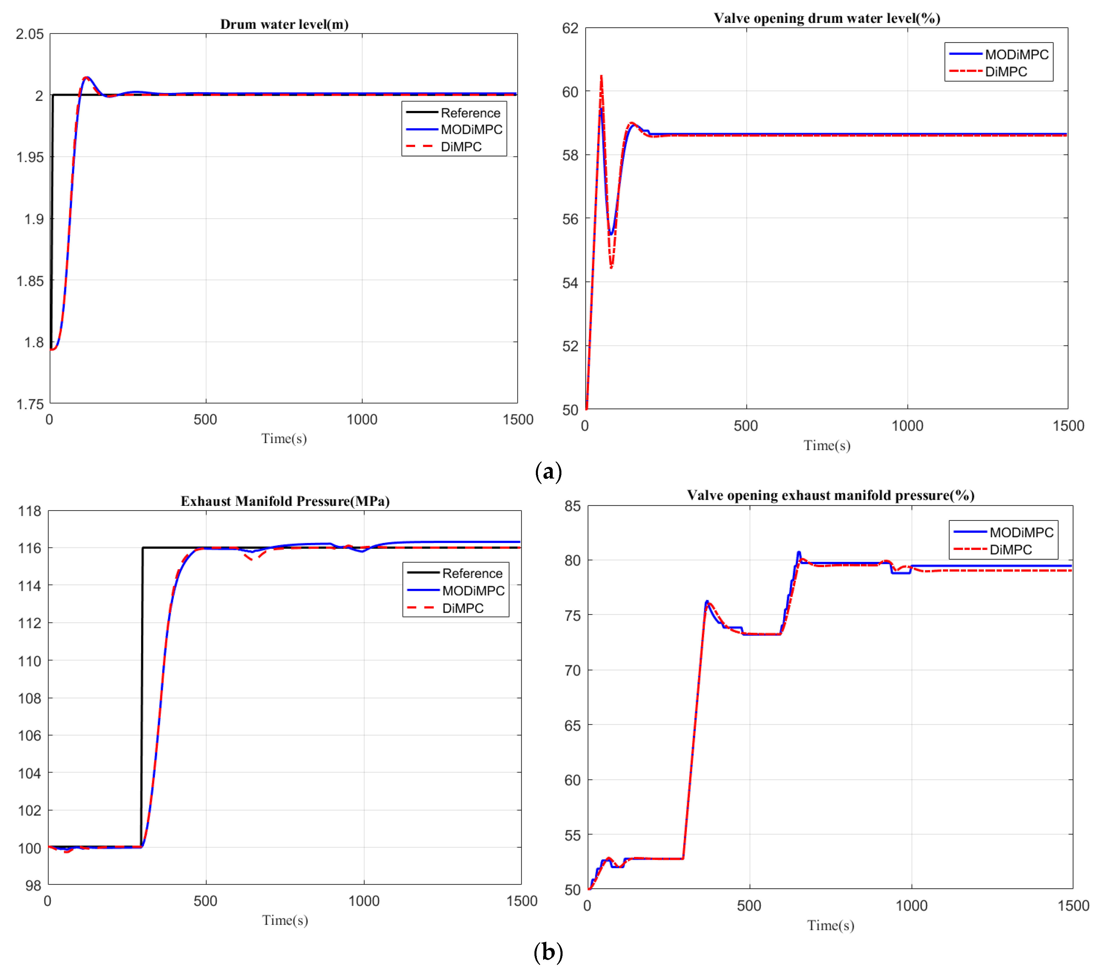
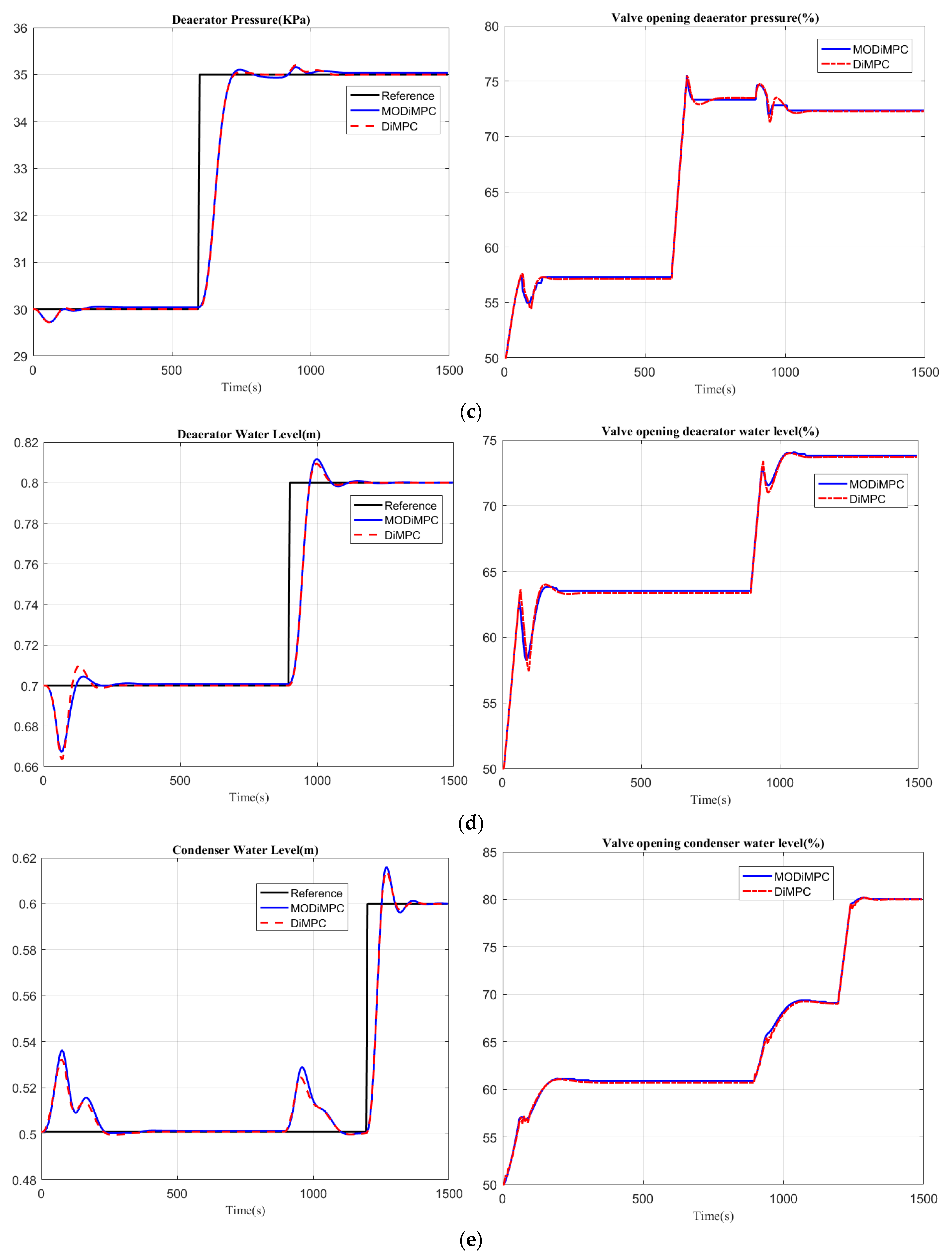
The results for the DiMPC and the multiple objective distributed model predictive control (MODiMPC) are shown in Figure 10. The performance indexes are shown in

Table 6. Performance indexes for IARE and ISU.

	MODiMPC	DiMPC
IARE	2.6289	2.5117
ISU	0.4434	0.4672

. The computing time for MODiMPC is 2.81 s and for the DiMPC 29.36 s, respectively.

It can be seen from the results that there is a large improvement in the computing time after the MODiMPC was applied and without too much loss in tracking performance.

As previously mentioned, in order to guarantee the stability of the optimal solution in a DiMPC framework, the convergence of the optimal solution was firstly discussed. Due to the fact that there are only constraints in input variables in our study, the feasibility of the steam/water loop belongs to the trivial case (according to [33], solving the optimization problem the existence of a feasible solution is ensured at each sampling period). The H_i matrices for the five loops are calculated as follows (for more details about convergence issue, please refer to the reference [33]):

$$\begin{gathered} H_1=\left[\begin{array}{cccc}0.9613& -0.0352& -0.0308& -0.0639\\ -0.0352& 0.9673& -0.0293& -0.0716\\ -0.0308& -0.0293& -0.9730& -0.0781\\ -0.0639& -0.0716& -0.0781& 0.2062\end{array}\right],H_2={0.0003,\mathrm{H}}_3=0.0025, \\ {\mathrm{H}}_4=\left[\begin{array}{cccc}0.9866& -0.0125& -0.0113& -0.0224\\ -0.0125& 0.9876& 0.0114& -0.0298\\ -0.0113& -0.0114& -0.9888& -0.0369\\ -0.0224& -0.0298& -0.0369& 0.4255\end{array}\right], \\ \begin{array}{l}{\mathrm{H}}_5=\left[\begin{array}{cccccc}0.9788& -0.0189& -0.0159& -0.0119& -0.0077& 0.0145\\ -0.0189& 0.9789& 0.0189& -0.0160& -0.0121& 0.0106\\ -0.0159& -0.0189& -0.9788& -0.0190& -0.0160& 0.0041\\ -0.0119& -0.0160& -0.0190& 0.9788& -0.0188& -0.0049\\ -0.0077& -0.0121& -0.0160& -0.0188& 0.9792& -0.0158\\ 0.0145& 0.0106& 0.0041& -0.0049& -0.0158& 0.4403\end{array}\right]\end{array} \end{gathered}$$

By the eig function in MATLAB (R2016b, Mathworks, Natick, MA, USA, 2016), the eigenvalues are calculated in a centralized manner for the steam/water loop, and the maximum value is ${\rho }_{\max }< 1$, which indicates that the DiMPC is convergent. In the steam/water loop, the five sub-loops cover the full system, and in the DiMPC the information is exchanged iteratively. Hence, the conditions 1 and 3–6 are satisfied. In order to cover the worst circumstances, the sufficient conditions in Section 3.5 tend to be conservative, and in some cases the convexity are not necessary [37]. Hence, it is concluded that the DiMPC has the same convergence as the CMPC, and the convergence of the DiMPC is guaranteed.

5. Conclusions

Regarding the multiple sub-loops in the steam/water loop, this paper introduced a distributed model predictive control based on the EPSAC framework. Different types of the MPC were applied to the steam/water loop system, including the DeMPC, CMPC and DiMPC. According to the simulation results, the DiMPC had similar performance with the CMPC, and outperformed the DeMPC. Due to the multiple controllers in the DiMPC strategy, the DiMPC had better performance of fault-tolerance and flexibility than the CMPC which improved the reliability of the steam/water loop. By proving equivalence in stability between the DiMPC and the CMPC, and the stability of the CPMC, the stability of the DiMPC is guaranteed. Meanwhile, a multiple objective MPC was proposed, and the computing speed was improved without too much loss in tracking performance.

References

- Mazur, K.; Wydra, M.; Ksiezopolski, B. Secure and time-aware communication of wireless sensors monitoring overhead transmission lines. Sensors 2017, 17, 1610. [Google Scholar] [CrossRef] [PubMed]
- Smierzchalski, R. Simulation system for marine engine control room. In Proceedings of the 2008 11th International Biennial Baltic Electronics Conference, Tallinn, Estonia, 6–8 October 2008; pp. 281–284. [Google Scholar]
- Vandermeulen, A.; van der Heijde, B.; Helsen, L. Controlling district heating and cooling networks to unlock flexibility: A review. Energy 2018, 151, 103–115. [Google Scholar] [CrossRef]
- Morstyn, T.; Hredzak, B.; Demetriades, G.D.; Agelidis, V.G. Unified distributed control for DC microgrid operating modes. IEEE Trans. Power Syst. 2016, 31, 802–812. [Google Scholar] [CrossRef]
- Maxim, A.; Copot, D.; Copot, C.; Ionescu, C.M. The 5W’s for Control as Part of Industry 4.0: Why, What, Where, Who, and When—A PID and MPC Control Perspective. Inventions 2019, 4, 10. [Google Scholar] [CrossRef]
- Copot, D.; Ghita, M.; Ionescu, C.M. Simple Alternatives to PID-Type Control for Processes with Variable Time-Delay. Processes 2019, 7, 146. [Google Scholar] [CrossRef]
- Haji, V.H.; Monje, C.A. Fractional order fuzzy-PID control of a combined cycle power plant using Particle Swarm Optimization algorithm with an improved dynamic parameters selection. Appl. Soft Comput. 2017, 58, 256–264. [Google Scholar] [CrossRef]
- Puchalski, B.; Duzinkiewicz, K.; Rutkowski, T. Multi-region fuzzy logic controller with local PID controllers for U-tube steam generator in nuclear power plant. Arch. Control Sci. 2015, 25, 429–444. [Google Scholar] [CrossRef] [Green Version]
- Magdy, G.; Mohamed, E.A.; Shabib, G.; Elbaset, A.A.; Mitani, Y. SMES based a new PID controller for frequency stability of a real hybrid power system considering high wind power penetration. IET Renew. Power Gener. 2018, 12, 1304–1313. [Google Scholar] [CrossRef]
- Salehi, A.; Safarzadeh, O.; Kazemi, M.H. Fractional order PID control of steam generator water level for nuclear steam supply systems. Nucl. Eng. Des. 2019, 342, 45–59. [Google Scholar] [CrossRef]
- Xi, Y.; Yu, X.; Wang, Y.; Li, Y.; Huang, J. Robust Nonlinear Adaptive Backstepping Coordinated Control for Boiler-Turbine Units. In Proceedings of the 2018 IEEE 27th International Symposium on Industrial Electronics (ISIE), Cairns, Australia, 13–15 June 2018; pp. 1167–1172. [Google Scholar]
- Cai, J.; Sun, L. Direct Fuzzy Backstepping Control for Turbine Main Steam Valve of Multi-machine Power System. In Proceedings of the 2015 2nd International Conference on Information Science and Control Engineering, Shanghai, China, 24–26 April 2015; pp. 702–706. [Google Scholar]
- Roy, T.K.; Mahmud, M.A.; Shen, W.; Oo, A.M. Non-linear adaptive coordinated controller design for multimachine power systems to improve transient stability. IET Gener. Trans. Distrib. 2016, 10, 3353–3363. [Google Scholar] [CrossRef]
- Rinaldi, G.; Cucuzzella, M.; Ferrara, A. Sliding mode observers for a network of thermal and hydroelectric power plants. Automatica 2018, 98, 51–57. [Google Scholar] [CrossRef]
- Kenne, G.; Fombu, A.M.; de Dieu Nguimfack-Ndongmo, J. Coordinated excitation and steam valve control for multimachine power system using high order sliding mode technique. Electr. Power Syst. Res. 2016, 131, 87–95. [Google Scholar] [CrossRef]
- Ansarifar, G.R.; Akhavan, H.R. Sliding mode control design for a PWR nuclear reactor using sliding mode observer during load following operation. Ann. Nucl. Energy. 2015, 75, 611–619. [Google Scholar] [CrossRef]
- Moradi, H.; Saffar-Avval, M.; and Bakhtiari-Nejad, F. Sliding mode control of drum water level in an industrial boiler unit with time varying parameters: A comparison with H∞-robust control approach. J. Process. Contr. 2012, 22, 1844–1855. [Google Scholar] [CrossRef]
- Ansarifar, G.R. Control of the nuclear steam generators using adaptive dynamic sliding mode method based on the nonlinear model. Ann. Nucl. Energy 2016, 88, 280–300. [Google Scholar] [CrossRef]
- Wu, J.; Nguang, S.K.; Shen, J.; Liu, G.; Li, Y.G. Robust H∞ tracking control of boiler-turbine systems. ISA Trans. 2010, 49, 369–375. [Google Scholar] [CrossRef] [PubMed]
- Ghabraei, S.; Moradi, H.; Vossoughi, G. Design & application of adaptive variable structure &H∞ robust optimal schemes in nonlinear control of boiler-turbine unit in the presence of various uncertainties. Energy 2018, 142, 1040–1056. [Google Scholar]
- Sun, L.; Li, D.; Hu, K.; Lee, K.Y.; Pan, F. On tuning and practical implementation of active disturbance rejection controller: A case study from a regenerative heater in a 1000 MW power plant. Ind. Eng. Chem. Res. 2016, 55, 6686–6695. [Google Scholar] [CrossRef]
- Sun, L.; Hua, Q.; Shen, J.; Xue, Y.; Li, D.; Lee, K.Y. Multi-objective optimization for advanced superheater steam temperature control in a 300 MW power plant. Appl. Energy 2017, 208, 592–606. [Google Scholar] [CrossRef]
- Sun, L.; Hua, Q.; Li, D.; Pan, L.; Xue, Y.; Lee, K.Y. Direct energy balance based active disturbance rejection control for coal-fired power plant. ISA Trans. 2017, 70, 486–493. [Google Scholar] [CrossRef]
- Zhang, F.; Wu, X.; Shen, J. Extended state observer based fuzzy model predictive control for ultra-supercritical boiler-turbine unit. Appl. Therm. Eng. 2017, 118, 90–100. [Google Scholar] [CrossRef]
- Kong, X.; Liu, X.; Lee, K.Y. Nonlinear multivariable hierarchical model predictive control for boiler-turbine system. Energy 2015, 93, 309–322. [Google Scholar] [CrossRef]
- Wu, X.; Shen, J.; Li, Y.; Lee, K.Y. Fuzzy modeling and predictive control of superheater steam temperature for power plant. ISA Trans. 2015, 56, 241–251. [Google Scholar] [CrossRef] [PubMed]
- Liu, X.; Cui, J. Economic model predictive control of boiler-turbine system. J. Process Control 2018, 66, 59–67. [Google Scholar] [CrossRef]
- Zhao, S.; Maxim, A.; Liu, S.; De Keyser, R.; Ionescu, C. Effect of Control Horizon in Model Predictive Control for Steam/Water Loop in Large-Scale Ships. Processes 2018, 6, 265. [Google Scholar] [CrossRef]
- Zhao, S.; Cajo, R.; De Keyser, R.; Liu, S.; Ionescu, C.M. Nonlinear predictive control applied to steam/water loop in large scale ships. In Proceedings of the 12th IFAC Symposium on Dynamics and Control of Process Systems, Including Biosystems, Florianopolis, Brazil, 24–26 April 2019. [Google Scholar]
- Gao, Z.; Saxen, H.; Gao, C. Special section on data-driven approaches for complex industrial systems. IEEE Trans. Ind. Inform. 2013, 9, 2210–2212. [Google Scholar] [CrossRef]
- Gao, Z.; Nguang, S.K.; Kong, D.X. Advances in Modelling, Monitoring, and Control for Complex Industrial Systems. Complexity 2019. [Google Scholar] [CrossRef]
- Venkat, A.N.; Rawlings, J.B.; Wright, S.J. Stability and optimality of distributed model predictive control. In Proceedings of the 44th IEEE Conference on Decision and Control, Seville, Spain, 15 December 2005; pp. 6680–6685. [Google Scholar]
- Maxim, A.; Copot, D.; De Keyser, R.; Ionescu, C.M. An industrially relevant formulation of a distributed model predictive control algorithm based on minimal process information. J. Process Control 2018, 68, 240–253. [Google Scholar] [CrossRef]
- De Keyser, R. Model based predictive control for linear systems, in: UNESCO Encyclopaedia of Life Support Systems. Control Syst. Robot. Autom. 2009, 11, 24–58. [Google Scholar]
- Camponogara, E.; Jia, D.; Krogh, B.H.; Talukdar, S. Distributed model predictive control. IEEE Control Syst. Mag. 2002, 22, 44–52. [Google Scholar]
- Camponogara, E. Controlling Networks with Collaborative Nets. Ph.D. Thesis, Carnegie Mellon University, Pittsburgh, PA, USA, 2000. [Google Scholar]
- Talukdar, S.; Camponogara, E. Collaborative nets. In Proceedings of the 33rd Annual Hawaii International Conference on System Sciences, Maui, HI, USA, 7 January 2000; p. 9. [Google Scholar]
- Starr, K.D. Single Loop Control Methods; ABB Inc.: Westerville, OH, USA, 2015. [Google Scholar]
Figure 1.
Scheme of a complete steam/water loop [28] (reproduced with permission from Zhao, S.; Maxim, A.; Liu, S.; De Keyser, R.; and Ionescu, C, Processes; published by MDPI, 2018).
Figure 2.
The normalized outputs of the steam/water loop with 10% step change in the input variables.
Figure 3.
Static gain under different input changes. (The figures on left hand indicate the static gain for drum water level loop, deaerator water level loop, and condenser water level loop; and on the right hand indicate the static gain for deaerator pressure loop, and exhaust manifold pressure loop).
Figure 4.
A conceptual representation of the centralized model predictive control (MPC) architecture [33] (Reproduced with permission from Maxim, A.; Copot, D.; De Keyser, R.; and Ionescu, C.M., Journal of Process Control; published by Elsevier, 2018).
Figure 5.
A conceptual representation of the distributed MPC architecture [33] (Reproduced with permission from Maxim, A.; Copot, D.; De Keyser, R.; and Ionescu, C.M., Journal of Process Control; published by Elsevier, 2018).
Figure 6.
A conceptual representation of the decentralized MPC architecture [33] (Reproduced with permission from Maxim, A.; Copot, D.; De Keyser, R.; and Ionescu, C.M., Journal of Process Control; published by Elsevier, 2018).
Figure 7.
Flow chart for the MODiMPC.
Figure 8.
The responses of the steam/water loop under the DeMPC, CMPC and DiMPC for (a) drum water level control loop, (b) deaerator water level control loop, (c) deaerator pressure control loop, (d) condenser water level control loop and (e) exhaust manifold pressure control loop (The figures on left hand indicate the outputs, and on the right hand indicate the inputs).
Figure 9.
The iteration times when the DiMPC is applied to the steam/ water loop.
Figure 10.
The responses of the steam/water loop under the MODiMPC and DiMPC for (a) drum water level control loop, (b) deaerator water level control loop, (c) deaerator pressure control loop, (d) condenser water level control loop and (e) exhaust manifold pressure control loop (The figures on left hand indicate the outputs, and on the right hand indicate the inputs).