Optimal Nonlinear Adaptive Control for Voltage Source Converters via Memetic Salp Swarm Algorithm: Design and Hardware Implementation

Abstract

Voltage source converter (VSC) has been extensively applied in renewable energy systems which can rapidly regulate the active and reactive power. This paper aims at developing a novel optimal nonlinear adaptive control (ONAC) scheme to control VSC in both rectifier mode and inverter mode. Firstly, the nonlinearities, parameter uncertainties, time-varying external disturbances, and unmodelled dynamics can be aggregated into a perturbation, which is then estimated by an extended state observer (ESO) called high-gain perturbation observer (HGPO) online. Moreover, the estimated perturbation will be fully compensated through state feedback. Besides, the observer gains and controller gains are optimally tuned by a recent emerging biology-based memetic salp swarm algorithm (MSSA), the utilization of such method can ensure a desirably satisfactory control performance. The advantage of ONAC is that even though the operation conditions are constantly changing, the control performance can still be maintained to be globally consistent. In addition, it is noteworthy that in rectifier mode only the reactive power and DC voltage are required to be measured, while in inverter mode merely the reactive power and active power have to be measured. At last, in order to verify the feasibility of ONAC in practical application, a hardware experiment is implemented.

1. Introduction

The rapidly growing energy demand has driven the fast deployment and development of renewable energy which involves advanced electronic devices to generate power. Generally speaking, such electrical power usually needs to be converted, e.g., DC (direct current)-DC(direct current) boost or buck, AC (alternating current)-DC (rectifier mode), DC-AC (inverter mode), etc., to provide a proper power supply to satisfy various power demanders. In the past decade, thanks to the advancement of modern electronics technology, studies on voltage source converters (VSC) utilizing insulated gate bipolar transistors (IGBT) have gained considerable attentions and interests around the globe [1]. VSC has many advantages over the conventional current source converter (CSC), e.g., decoupled control of the active power and reactive power and the communication process can successfully be achieved without external voltage source supply. Several typical VSC applications can be traced to VSC-based high voltage direct current (VSC-HVDC) systems [2], doubly fed induction generation (DFIG) [3], permanent magnetic synchronous generator (PMSG) [4], and photovoltaic (PV) inverter [5]. So far, VSC plays a major role in distributed generation (DG) systems [6,7,8] to ensure a reliable power supply.

In practice, it often requires VSC to operate rapidly to ensure the reactive power and DC voltage can be regulated in time when it operates at rectifier mode, while achieving the regulation of the reactive power and active power when it operates at inverter mode. Hence, the proper design of control systems plays an important role in VSC operation. Conventional proportional–integral–derivative (PID) control has acquired wide applications, since the one-point linearization is always used when the control parameters are tuned, once the operation points change the overall control performance of PID controller may decline significantly [9]. Such issue become particularly severe for DG systems as they often operate under stochastic atmospheric conditions, such as random wind speed variation, solar irradiation, and temperature change.

To resolve this challenging issue, many advanced control strategies have been developed, such as feedback linearization control (FLC) [10] applied in VSC-HVDC systems, which fully removes the nonlinearities of the system to guarantee a global control consistency under different operation conditions. Nevertheless, FLC requires a system model which can precisely describe the characteristics of the system and fully state measurements, thus it lacks robustness for the parameters of ideal model change and is difficult to be implemented in practice. To enhance the robustness, sliding-mode control (SMC) [11] was applied to VSC-HVDC system. However, chattering may emerge from SMC due to the use of discontinuous functions in the controller loop, together with an increased scale of controller structure complexity. Meanwhile, in reference [12], a passivity-based sliding-mode control (PBSMC) scheme was employed for rotor-side VSC of PMSG to efficiently undertake maximum power point tracking (MPPT) under different wind profiles. However, it requires many state measurements and an accurate system model which is hard to achieve in reality, thus making its implementation questionable. Moreover, a robust sliding-mode control (RSMC) strategy was developed on the rotor-side VSC of DFIG to enhance the robustness under modelling uncertainties [13], which largely increased the complexity and resulted in an overconservativeness due to the upper bound of perturbation used, which does not often occur in practice. In addition, model predictive control (MPC) has been applied on PV inverters to achieve a rapid power regulation in the presence of modelling uncertainties [14], which, however, needs to employ extra control loops, thus, the system complexity becomes significant. Besides, literature [15] adopted an effective control strategy, in which a disturbance estimator-based predictive current controller is utilized for PV inverters to estimate the unknown PV inverter parameters and modelling uncertainties. However, it introduces a large number of estimator gains for which tuning is difficult.

Basically, the aforementioned nonlinear approaches have a relatively complex structure, thus their implementation is usually difficult. Based on extended state observer (ESO) [16,17,18], a nonlinear adaptive control (NAC) strategy for VSC operating in both rectifier mode and inverter mode is proposed in this paper. The combined influence of system nonlinearities, uncertain parameters, unmodelled dynamics, and time-varying external disturbances can be synthesized into a perturbation, which can be estimated through a high-gain perturbation observer (HGPO) [19,20,21]. NAC only requires the measurement of DC voltage and reactive power for rectifier mode, and active power and reactive power for inverter mode. Thus, it provides the merit of inherently easy implementation in real systems.

However, NAC involves many parameters that need to be properly tuned, e.g., (a) observer gains which determine the perturbation estimation performance and (b) controller gains which influence the control performance. These gains are interactively coupled, thus, the optimal tuning of them is worth studying. To handle this issue, this paper aimed to design an optimal NAC (ONAC) strategy to achieve optimal parameter tuning of NAC for VSC, such that an optimal and robust control can be achieved under different operation scenarios. In particular, a newly emerging biology based metaheuristic algorithm was utilized, called memetic salp swarm algorithm (MSSA) [22], to tune the parameters of NAC more optimally and efficiently, such that the control performance of NAC can be optimized. More specifically, the salp chains adopted by MSSA are multiple independent ones, such a strategy can better balance exploration and exploitation, thus, a high-quality optimum can be efficiently found. Besides this, a novel regroup operation using a virtual population is employed to globally coordinate different salp chains, such that the convergence stability can be considerably improved.

Lastly, the proposed ONAC is compiled and downloaded into the dSPACE processor as the real-time controller for VSC, in which the I/O interface of dSPACE simulator enables the real-time sampling of inputs from measurements and output control signals with IGBT converters. Several case studies were done to verify the hardware practicality of ONAC based inverter controller and rectifier controller.

The originality and novelty of this work can be summarized as follows:

(a)

The large parameter tuning burden of conventional NAC can be efficiently resolved via MSSA, which can efficiently and effectively seek the optimal controller and observer parameters with a high stability;

(b)

Various modelling uncertainties can be effectively estimated by HGPO in the real-time, which is then fully compensated by the controller online, such that great robustness can be realized;

(c)

A dSpace based hardware experiment was undertaken which validates the implementation feasibility of ONAC.

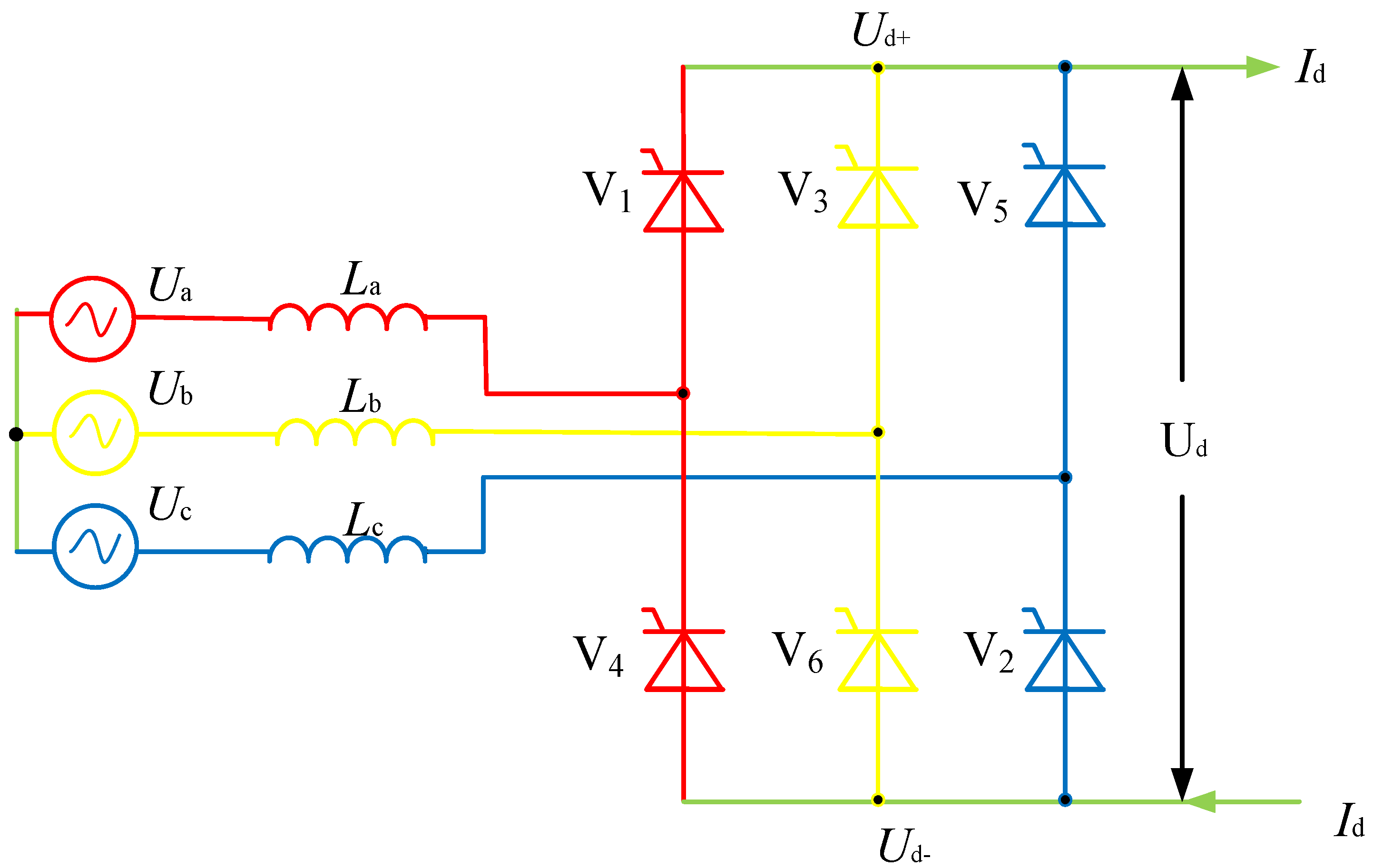
The structure of this paper is organized as follows: Section 2 presents the VSC modelling; Section 3 provides the ONAC design; in Section 4, ONAC design for VSC is given; Section 5 presents the experimental results of ONAC; lastly, Section 6 concludes the whole paper.

2. VSC Modelling

VSC can be operated in either rectifier mode (which can achieve the regulation of the reactive power and DC voltage) or inverter mode (which can achieve the regulation of the reactive power and active power). Figure 1 presents a typical structure of VSC. Here, the balanced condition has been taken into consideration, i.e., the parameters of three phases on the AC side are totally the same and the amplitude of voltages and currents are identical, while each phase shifts 120° between themselves. When the angular frequency is ω, the rectifier dynamics in d-q rotational frame can be expressed as [9]:

$$\{\begin{array}{c}\frac{\mathrm{d}{i}_{\mathrm{d}1}}{\mathrm{d}t}=-\frac{R_1}{L_1}{i}_{\mathrm{d}1}+\omega i_{\mathrm{q}1}+u_{\mathrm{d}1}\\ \frac{\mathrm{d}{i}_{\mathrm{q}1}}{\mathrm{d}t}=-\frac{R_1}{L_1}{i}_{\mathrm{q}1}-\omega i_{\mathrm{d}1}+u_{\mathrm{q}1}\\ \frac{\mathrm{d}{V}_{\mathrm{dc}1}}{\mathrm{d}t}=\frac{3u_{\mathrm{sq}1}{i}_{\mathrm{q}1}}{2C_1{V}_{\mathrm{dc}1}}-\frac{i_{\mathrm{L}}}{C_1}\end{array}$$

(1)

where the rectifier is linked to the AC grid by the equivalent resistance R₁ and inductance L₁, respectively, C₁ represents the capacitance of DC bus, $u_{\mathrm{d}1}=\frac{u_{\mathrm{sd}1}-u_{\mathrm{rd}}}{L_1}$ and $u_{\mathrm{q}1}=\frac{u_{\mathrm{sq}1}-u_{\mathrm{rq}}}{L_1}$. $i_{\mathrm{L}}$ denotes the DC current that flows out of the rectifier.

The inverter dynamics in d-q rotational frame are written as:

$$\{\begin{array}{c}\frac{\mathrm{d}{i}_{\mathrm{d}2}}{\mathrm{d}t}=-\frac{R_2}{L_2}{i}_{\mathrm{d}2}+\omega i_{\mathrm{q}2}+u_{\mathrm{d}2}\\ \frac{\mathrm{d}{i}_{\mathrm{q}2}}{\mathrm{d}t}=-\frac{R_2}{L_2}{i}_{\mathrm{q}2}-\omega i_{\mathrm{d}2}+u_{\mathrm{q}2}\\ \frac{\mathrm{d}{V}_{\mathrm{dc}2}}{\mathrm{d}t}=\frac{3u_{\mathrm{sq}2}{i}_{\mathrm{q}2}}{2C_2{V}_{\mathrm{dc}2}}+\frac{i_{\mathrm{L}}}{C_2}\end{array}$$

(2)

where the inverter is linked to the AC grid by the equivalent resistance R₂ and inductance L₂, respectively, C₂ represents the capacitance of DC bus, $u_{\mathrm{d}2}=\frac{u_{\mathrm{sd}2}-u_{\mathrm{rd}}}{L_2}$ and $u_{\mathrm{q}2}=\frac{u_{\mathrm{sq}2}-u_{\mathrm{rq}}}{L_2}$.$i_{\mathrm{L}}$ denotes the DC current that flows into the inverter.

On the rectifier side, the q-axis is defined to share the same phase with the AC grid voltage u_s1. Similarly, the q-axis and the AC grid voltage u_s2 are defined to share the same phase on the inverter side. Under this circumstance, the values of u_sd1 and u_sd2 can be regarded as 0, while the values of u_sq1 and u_sq2 are deemed as identical with the magnitude of u_s1 and u_s2. Hence, the reactive and active power can be described by

$$\{\begin{array}{l}{P}_1=\frac{3}{2}\left(u_{\mathrm{sq}1}{i}_{\mathrm{q}1}+u_{\mathrm{sd}1}{i}_{\mathrm{d}1}\right)=\frac{3}{2}{u}_{\mathrm{sq}1}{i}_{\mathrm{q}1}\\ Q_1=\frac{3}{2}\left(u_{\mathrm{sq}1}{i}_{\mathrm{d}1}+u_{\mathrm{sd}1}{i}_{\mathrm{q}1}\right)=\frac{3}{2}{u}_{\mathrm{sq}1}{i}_{\mathrm{d}1}\\ P_2=\frac{3}{2}\left(u_{\mathrm{sq}2}{i}_{\mathrm{q}2}+u_{\mathrm{sd}2}{i}_{\mathrm{d}2}\right)=\frac{3}{2}{u}_{\mathrm{sq}2}{i}_{\mathrm{q}2}\\ Q_2=\frac{3}{2}\left(u_{\mathrm{sq}2}{i}_{\mathrm{d}2}+u_{\mathrm{sd}2}{i}_{\mathrm{q}2}\right)=\frac{3}{2}{u}_{\mathrm{sq}2}{i}_{\mathrm{d}2}\end{array}.$$

(3)

3. Optimal Nonlinear Adaptive Control

3.1. Nonlinear Adaptive Control

The standard form of an uncertain nonlinear system can be expressed as follows:

$$\{\begin{array}{c}\dot{x}=Ax+B\left(a\left(x\right)+b\left(x\right)u+d\left(t\right)\right)\\ y=x_1\end{array}$$

(4)

where $x={\left[x_1,x_2,\cdots ,x_n\right]}^{\mathrm{T}}\in R^n$ represents the state variable vector; $y\in R$ and $u\in R$ denote the system output and control input, respectively; a(x): $R^n\mapsto R$ and b(x): $R^n\mapsto R$ represent the unknown smooth functions which describe the aggregation influence of nonlinearities, parameter uncertainties, and unmodelled dynamics; and d(t): $R^{+}\mapsto R$ means the time-varying external disturbances.

The perturbation of system (4) can be obtained by [19,20,21]

$$\psi \left(x,u,t\right)=a\left(x\right)+\left(b\left(x\right)-b_0\right)u+d\left(t\right)$$

(5)

where b₀ represents a constant control gain defined by users, by which the uncertainties of the control gain b(x) can be synthesized into the perturbation.

From system (4), the final state, e.g., x_n, can be further expressed as

$${\dot{x}}_n=a\left(x\right)+\left(b\left(x\right)-b_0\right)u+d\left(t\right)+b_{0}u=\psi \left(x,u,t\right)+b_{0}u.$$

(6)

Besides, the perturbation term can be expressed by defining an extended state, e.g., $x_{n+1}=\psi \left(x,u,t\right)$. Further, system (4) can be described by

$$\{\begin{array}{c}y=x_1\\ {\dot{x}}_1=x_2\\ ⋮\\ {\dot{x}}_n=x_{n+1}+b_{0}u\\ {\dot{x}}_{n+1}=\dot{\psi }(·)\end{array}.$$

(7)

Under the two assumptions given in [19,20,21], the extended state vector can be represented by $x_{\mathrm{e}}={\left[x_1,x_2,\cdots ,x_n,x_{n+1}\right]}^{\mathrm{T}}$.

A.1

The selection of b₀ needs to satisfy certain constraint: $\left|b\left(x\right)/b_0-1\right|\le \theta <1$, where θ is a positive constant.

A.2

The function $\psi \left(x,u,t\right):R^n\times R\times R^{+}\mapsto R$ and $\dot{\psi }\left(x,u,t\right):R^n\times R\times R^{+}\mapsto R$ are locally Lipschitz in their arguments with a bounded domain of interest, with $\psi$ (0,0,0) = 0 and $\dot{\psi }$ (0,0,0) = 0.

In this paper, $\tilde{x}=x-\widehat{x}$ denotes the estimation error of x and $\widehat{x}$ means the estimation of x, while x* represents the reference of variable x. We designed an (n + 1)th-order HGSPO (high-gain state and perturbation observer) for the expanded system (8) to evaluate the states and perturbation at the same time, as follows [19,20,21]

$${\dot{\widehat{x}}}_{\mathrm{e}}=A_0{\widehat{x}}_{\mathrm{e}}+B_{1}u+H\left(x_1-{\widehat{x}}_1\right)$$

(8)

where $H={\left[{\alpha }_1/\epsilon ,{\alpha }_2/{\epsilon }^2,\dots ,{\alpha }_n/{\epsilon }^n,{\alpha }_{n+1}/{\epsilon }^{n+1}\right]}^{\mathrm{T}}$, thickness layer boundary of observer $0\le \epsilon \ll 1$, thus a high-gain can be successfully obtained in this way; and α_i, i = 1, 2, $\cdots$, n + 1 represents the gains of Luenberger observer—proper choice of its value can help to ensure the poles of polynomial sⁿ⁺¹ + α₁sⁿ + α₂sⁿ⁻¹ + $\cdots$ + α_n+1 = (s + ${\lambda }_{\alpha }$)ⁿ⁺¹ = 0 are located at the open left-half complex plane at −λ_α, as follows

$${\alpha }_i=C_{n+1}^i{\lambda }_{\alpha }^i,i=1,2,\cdots ,n+1$$

(9)

where λ_α represents the observer root utilized for ensuring the convergence of observer.

The NAC for system (4) under the estimation of states and perturbation can be written as

$$u=\frac{1}{b_0}\left[x_1^{*\left(n+1\right)}-\widehat{\psi }(·)-K\left(\widehat{x}-x^{*}\right)\right]$$

(10)

where $K=\left[k_1,k_2,\cdots ,k_n\right]$ represents the feedback control gain which makes the matrix A₁ = A-BK Hurwitzian.

Note that the closed-loop system stability of NAC has been provided in previous studies, interested readers can refer to literatures [19,20,21] for more details.

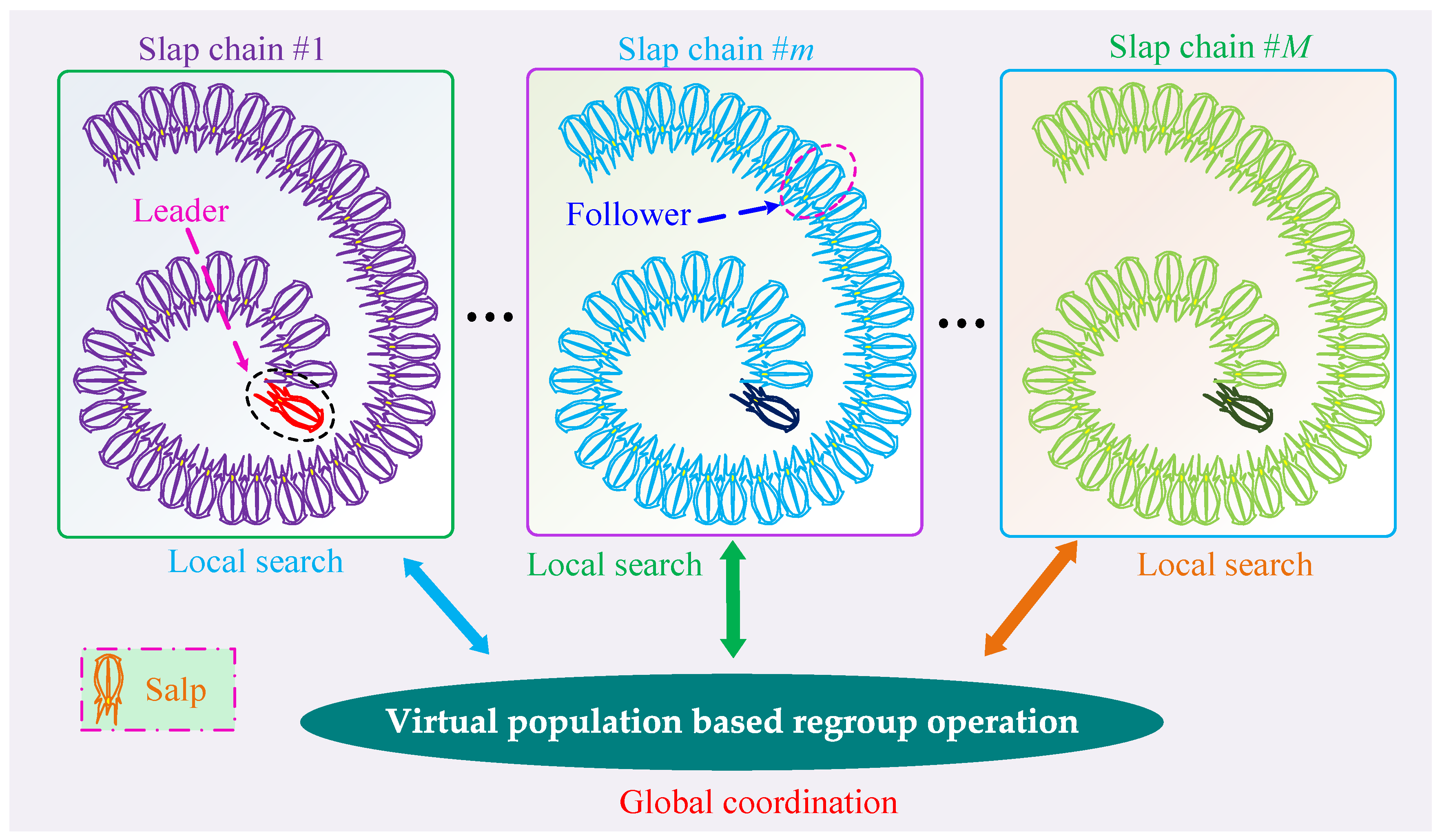
3.2. Memetic Salp Swarm Algorithm

MSSA is an emerging and promising metaheuristic algorithm which mimics the food hunting behavior of salp chains in deep oceans. Note that only the main idea of MSSA is presented in this section while more details are introduced in literature [21] for interested readers.

3.2.1. Optimization Framework

The memetic computing framework is utilized in MSSA for the purpose of improving the searching efficiency of SSA, which consists of two steps shown in Figure 2, as follows [22]:

• Local search in each chain: Several various salp chains are connected in parallel to constitute MSSA, in which a single salp chain consists of a host of salps. At each iteration, on the basis of foraging behavior of SSA, all the salp chains will undertake a local search while this process is independently carried out in each salp chain.
• Global coordination in virtual population: The whole species group of MSSA can merely be considered as a large number of memes, in which each meme is deemed as a unit of cultural evolution [23]. In particular, positive strategy is adopted in the selection of memes to enhance the communication ability among the salps in MSSA (memetic salp swarm algorithm). Besides, each individual can keep its own physical characteristics stable during the process of global coordination. Therefore, the salps gather together can be considered as a virtual population, where all individuals need to rearrange into many new salp chains, thus various salp chains can achieve a global coordination.

3.2.2. Local Search in Each Chain

The salp chain is composed of two groups, i.e., leader and follower. As illustrated by Figure 2, the leader always stays at the first position of the chain to decide the moving direction of the swarm, while all the other salps act as the followers to execute the command. In SSA (salp swarm algorithm), the position of each salp can be mathematically represented. Basically, the leader’s position in the mth salp chain during the foraging process is expressed as [24]:

$$x_{m1}^j=\{\begin{array}{c}{F}_m^j+c_1\left(c_2\left(u{b}^j-l{b}^j\right)+l{b}^j\right),\mathrm{if}{c}_3\ge 0\\ F_m^j-c_1\left(c_2\left(u{b}^j-l{b}^j\right)+l{b}^j\right),\mathrm{if}{c}_3<0\end{array}$$

(11)

where the superscript j denotes the jth dimension of the searching space; $x_{m1}^j$ represents the leader’s position in the mth salp chain; $F_m^j$ means the position of the food source; $l{b}^j$ and $u{b}^j$ represent the lower and the upper bounds of the jth dimension, respectively; $c_1$, $c_2$, and $c_3$ represent the random numbers, while $c_2$ and $c_3$ are uniformly distributed in the range of 0–1, respectively.

Since $c_1$ acts as the most vital parameter in Equation (11) as it directly influences the trade-off between global exploration and local exploitation, for the purpose of realizing a more appropriate balance, it has been designed based on the iteration number, which can be written as [24]:

$$c_1=2e^{-{\left(\frac{4k}{k_{\max }}\right)}^2}.$$

(12)

where k represents the number of current iteration and k_max denotes the maximum iteration number.

Moreover, the position of the followers is updated as follows [24]:

$$x_{mi}^j=\frac{1}{2}\left(x_{mi}^j+x_{m,i-1}^j\right),i=2,3,\dots ,n;m=1,2,\dots ,M$$

(13)

where $x_{mi}^j$ represents the position of the ith salp in the mth salp chain; n denotes the population size of each salp chain; and M means the salp chains number, respectively.

3.2.3. Global Coordination in Virtual Population

For the purpose of enhancing the stability of convergence, the virtual population need to be rearranged and generate various new salp chains based on the fitness values of the salps. In particular, the regroup operation of the original population in MSSA is achieved according to the classical memetic algorithm called shuffled frog leaping algorithm (SFLA) [25], which is a widely utilized population partition principle. Therefore, through arranging the fitness value in descending order the maximum optimization of regroup operation can be realized. Here, the best solution is allocated to the salp chain #1, then the salp chain #2 will capture the second-best solution, and so on. Hence, the mth salp chain can update the swarm according to

$$\begin{array}{c}{Y}^m=\{\left(x_{mi},f_{mi}\right)|x_{mi}=X\left(m+M\left(i-1\right),:\right),f_{mi}=F\left(m+M\left(i-1\right)\right),\\ i=1,2,\cdots ,n\},m=1,2,\cdots ,M\end{array}$$

(14)

where $x_{mi}$ represents the position vector of the ith salp in the mth chain; $f_{mi}$ denotes the fitness value of the ith salp in the mth chain; F means the fitness value set of all the salps in descending order; and X represents the relevant position vector set of all the salps, i.e., a position matrix, by

$$X=\left[\begin{array}{ccc}{x}_1^1& x_1^2& \begin{array}{cc}\cdots & x_1^d\end{array}\\ x_2^1& x_2^2& \begin{array}{cc}\cdots & x_2^d\end{array}\\ \begin{array}{c}⋮\\ x_{n\times M}^1\end{array}& \begin{array}{c}⋮\\ x_{n\times M}^2\end{array}& \begin{array}{cc}\begin{array}{c}\ddots \\ \dots \end{array}& \begin{array}{c}⋮\\ x_{n\times M}^d\end{array}\end{array}\end{array}\right]$$

(15)

where d represents the number of dimensions; and each row vector denotes the position vector of each salp.

3.2.4. Optimization Procedure of MSSA

In conclusion,

Table 1. The optimization procedure of MSSA (memetic salp swarm algorithm).

1. Initialize the optimization parameters; 2. Determine the fitness function according to the specific optimization problem; 3. Set k: = 1; 4. WHILE (the termination condition is not met) 5.     FOR1 m: = 1 to M 6.        FOR2 i: = 1 to n 7.           Calculate the fitness value of the ith salp in the mth salp chain; 8.        END FOR2 9.     END FOR1 10.    Implement the regroup operation based global coordination in virtual population by (14) and (18); 11.     FOR3 m: = 1 to M 12.        Determine the food source of the mth salp chain; 13.        Update the position of the leader in the mth salp chain by (13) and (12); 14.        FOR4 i: = 2 to n 15.           Update the position of the ith salp (i.e., the follower) in the mth salp chain by (13); 16.        END FOR4 17.     END FOR3 18.     Set k: = k + 1; 19. END WHILE

demonstrates the overall process of MSSA. When solving a practical optimization issue, the design of fitness function takes on the most important part in the whole procedure, and it needs to take the related objective function and constraints into consideration.

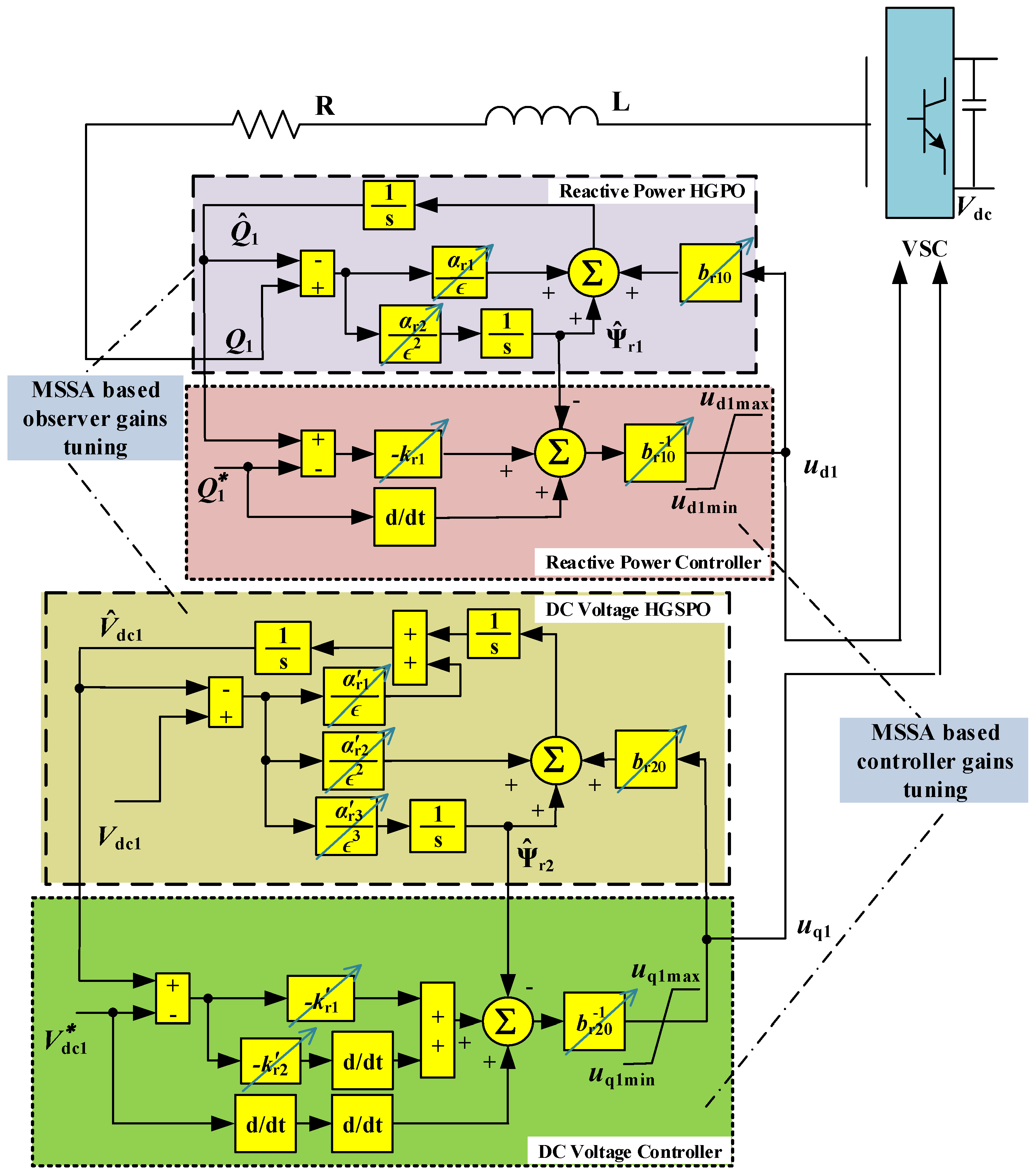
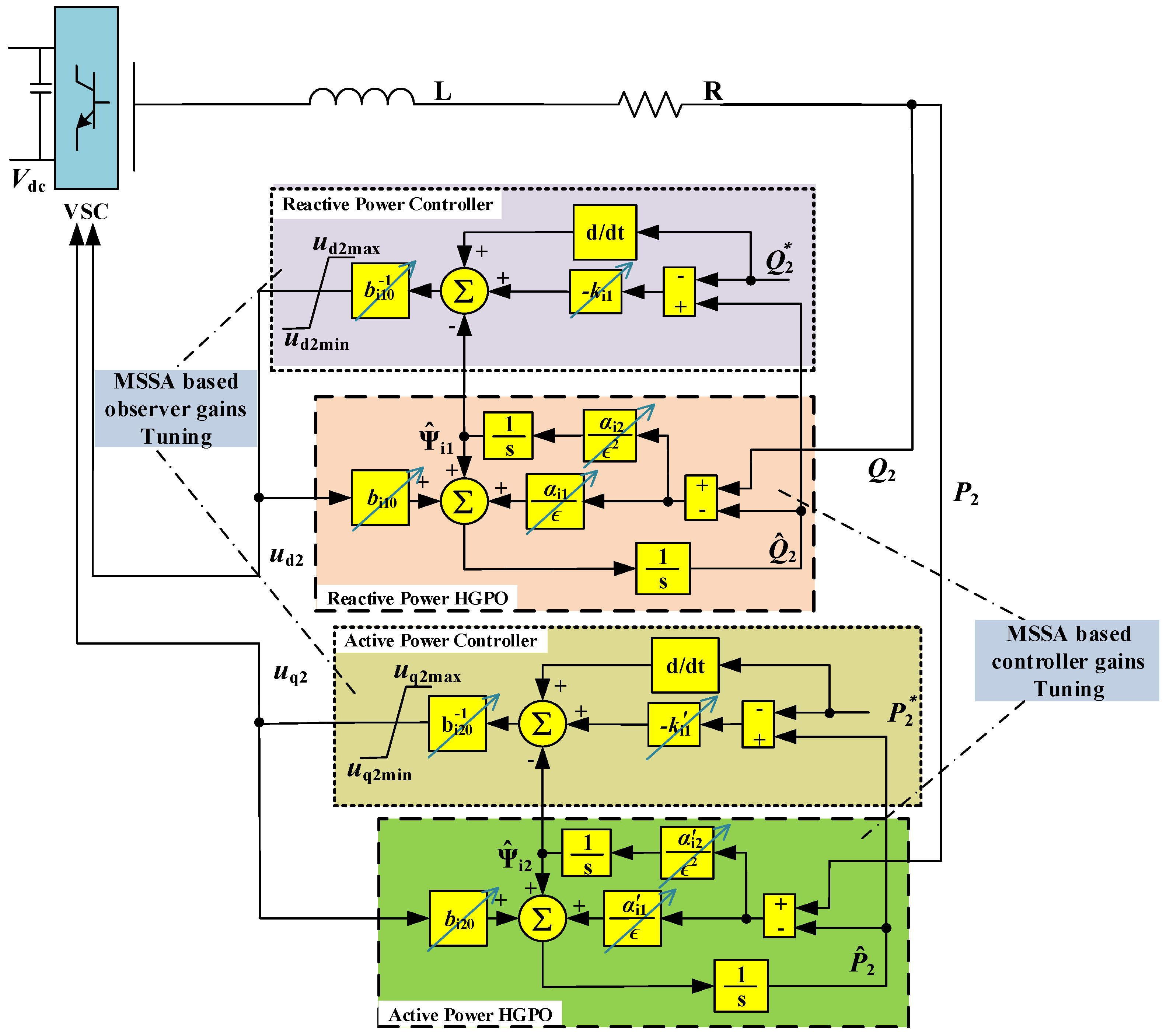
4. ONAC Design for VSC Based Rectifier and Inverter

4.1. Rectifier Controller Design

Select system output y_r = [y_r1, y_r2 ]^T = [Q₁, V_dc1]^T, ${\mathrm{Q}}_1^{*}$ and ${\mathrm{V}}_{\mathrm{dc}1}^{*}$ act as the given references of the DC voltage and reactive power, respectively. Throughout this paper, denote ${\widehat{x}}_i$ and ${\tilde{x}}_i=x_i-{\widehat{x}}_i$ as the estimate and estimate error of system state x_i, respectively. Define the tracking error as e_r = [e_r1, e_r2]^T = [Q₁- ${\mathrm{Q}}_1^{*}$, V_dc1- ${\mathrm{V}}_{\mathrm{dc}1}^{*}$]^T, differentiate e_r for rectifier (1) and repeat such operation until the control input can appear clearly, as follows

$$\left[\begin{array}{l}{\dot{e}}_{\mathrm{r}1}\\ {\ddot{e}}_{\mathrm{r}2}\end{array}\right]=\left[\begin{array}{l}{f}_{\mathrm{r}1}-{\dot{Q}}_1^{*}\\ f_{\mathrm{r}2}-{\ddot{V}}_{\mathrm{dc}1}^{{}^{*}}\end{array}\right]+B\mathrm{r}\left[\begin{array}{l}{u}_{\mathrm{d}1}\\ u_{\mathrm{q}1}\end{array}\right]$$

(16)

where

$$\{\begin{array}{l}{f}_{\mathrm{r}1}=\frac{3u_{\mathrm{sq}1}}{2}\left(-\frac{R_1}{L_1}{i}_{\mathrm{d}1}+\omega i_{\mathrm{q}1}\right)\\ f_{\mathrm{r}2}=\frac{3u_{\mathrm{sq}1}}{2C_1{V}_{\mathrm{dc}1}}\left[-\omega i_{\mathrm{d}1}-\frac{R_1}{L_1}{i}_{\mathrm{q}1}-\frac{i_{\mathrm{q}1}}{V_{\mathrm{dc}1}}\left(\frac{3u_{\mathrm{sq}1}{i}_{\mathrm{q}1}}{2C_1{V}_{\mathrm{dc}1}}-\frac{i_{\mathrm{L}}}{C_1}\right)\right]-\\ \frac{1}{2R_0{C}_1}\left(\frac{3u_{\mathrm{sq}1}{i}_{\mathrm{q}1}}{2C_1{V}_{\mathrm{dc}1}}-\frac{i_{\mathrm{L}}}{C_1}-\frac{3u_{\mathrm{sq}2}{i}_{\mathrm{q}2}}{2C_2{V}_{\mathrm{dc}2}}-\frac{i_{\mathrm{L}}}{C_2}\right)\end{array}$$

(17)

and

$$B\mathrm{r}=\left[\begin{array}{cc}\frac{3u_{\mathrm{sq}1}}{2L_1}& 0\\ 0& \frac{3u_{\mathrm{sq}1}}{2C_1{L}_1{V}_{\mathrm{dc}1}}\end{array}\right].$$

(18)

The determinant of matrix B_r is obtained as $\left|B_{\mathrm{r}}\right|=9u_{\mathrm{sq}1}^2/\left(4C_1{L}_1^2{V}_{\mathrm{dc}1}\right)$, which is nonzero in the entire operation range of the rectifier. Note that the only condition for zero value of $\left|B_{\mathrm{r}}\right|$ is that u_sq1 = 0, such condition corresponds to the case that the connected AC power grid voltage becomes zero. In practice, when the power gird voltage is below 0.2 p.u., the protection devices of VSC are activated and disconnect/stop the VSC working [8,9]. It is the same to $\left|B_{\mathrm{i}}\right|$ under inverter mode. As a result, VSC will not encounter this extreme case in practice. Hence, the system (16) can be regarded as linearizable, let v_r = [ v_r1, v_r2]^T be the control input of the linear system

$$\left[\begin{array}{c}{v}_{\mathrm{r}1}\\ v_{\mathrm{r}2}\end{array}\right]=-\left[\begin{array}{c}{k}_{\mathrm{r}1}{e}_{\mathrm{r}1}\\ k_{\mathrm{r}1}^{\prime }{e}_{\mathrm{r}2}+k_{\mathrm{r}2}^{\prime }{\dot{e}}_{\mathrm{r}2}\end{array}\right]$$

(19)

where k_r1, $k_{r1}^{\prime }$, and ${\mathrm{k}}_{\mathrm{r}2}^{\prime }$ represent the positive feedback gains.

Under the assumption that the nonlinearities are all unknown, the perturbations Ψ_r1(·) and Ψ_r2(·) can be written as

$$\left[\begin{array}{l}\Psi \mathrm{r}1(\cdot )\\ \Psi \mathrm{r}2(\cdot )\end{array}\right]=\left[\begin{array}{l}f\mathrm{r}1\\ f\mathrm{r}2\end{array}\right]+(B\mathrm{r}-B\mathrm{r}0)\left[\begin{array}{c}{u}_{\mathrm{d}1}\\ u_{\mathrm{q}1}\end{array}\right]$$

(20)

where the constant control gain B_r0 can be expressed as

$$B\mathrm{r}0=\left[\begin{array}{cc}b\mathrm{r}10& 0\\ 0& b\mathrm{r}20\end{array}\right].$$

(21)

Then, system (16) can be represented by

$$\left[\begin{array}{l}{\dot{e}}_{\mathrm{r}1}\\ {\ddot{e}}_{\mathrm{r}2}\end{array}\right]=\left[\begin{array}{l}\Psi r1(\cdot )\\ \Psi r2(\cdot )\end{array}\right]+Br0\left[\begin{array}{l}{u}_{d1}\\ u_{q1}\end{array}\right]-\left[\begin{array}{l}{\dot{Q}}_1^{*}\\ {\ddot{V}}_{dc1}^{*}\end{array}\right].$$

(22)

Define z₁₁ = Q₁, a second-order HGPO is given by

$$\{\begin{array}{l}{\dot{\widehat{z}}}_{11}=\widehat{\Psi }\mathrm{r}1(\cdot )+\frac{\alpha \mathrm{r}1}{\epsilon }(z_{11}-{\widehat{z}}_{11})+b\mathrm{r}10u_{\mathrm{d}1}\\ {\dot{\widehat{\Psi }}}_{\mathrm{r}1}(\cdot )=\frac{\alpha \mathrm{r}2}{{\epsilon }^2}(z_{11}-{\widehat{z}}_{11})\end{array}.$$

(23)

Define $z_{11}^{\prime }=V_{\mathrm{dc}1}$ and $z_{12}^{\prime }={\dot{z}}_{11}^{\prime }$, a third-order high-gain state and perturbation observer (HGSPO) is obtained by

$$\{\begin{array}{l}{{\dot{\widehat{z}}}^{\prime }}_{11}={{\widehat{z}}^{\prime }}_{12}+\frac{{{\alpha }^{\prime }}_{\mathrm{r}1}}{\epsilon }({z^{\prime }}_{11}-{{\widehat{z}}^{\prime }}_{11})\\ {{\dot{\widehat{z}}}^{\prime }}_{12}={\widehat{\Psi }}_{\mathrm{r}2}(\cdot )+\frac{{{\alpha }^{\prime }}_{\mathrm{r}2}}{{\epsilon }^2}({z^{\prime }}_{11}-{{\widehat{z}}^{\prime }}_{11})+\mathrm{br}20u\mathrm{q}1\\ {\dot{\widehat{\Psi }}}_{\mathrm{r}2}(\cdot )=\frac{{{\alpha }^{\prime }}_{\mathrm{r}3}}{{\epsilon }^3}({z^{\prime }}_{11}-{{\widehat{z}}^{\prime }}_{11})\end{array}$$

(24)

where $\alpha \mathrm{r}1$, $\alpha \mathrm{r}2$, ${{\alpha }^{\prime }}_{\mathrm{r}1}$, ${{\alpha }^{\prime }}_{\mathrm{r}2}$, and ${{\alpha }^{\prime }}_{\mathrm{r}3}$ represent positive constants with 1 $\gg ϵ>0$.

The NAC-based rectifier controller based on the estimations of perturbation can be given by

$$\left[\begin{array}{l}{u}_{\mathrm{d}1}\\ u_{\mathrm{q}1}\end{array}\right]=B_{\mathrm{r}0}^{-1}\left(\left[\begin{array}{l}-\widehat{\Psi }\mathrm{r}1(\cdot )\\ -\widehat{\Psi }\mathrm{r}2(\cdot )\end{array}\right]+\left[\begin{array}{l}{\dot{Q}}_1^{*}\\ {\ddot{V}}_{\mathrm{dc}1}^{{}^{*}}\end{array}\right]+v_{\mathrm{r}}\right).$$

(25)

4.2. Inverter Controller Design

Select system output y_i = [y_i1, y_i2]^T = [Q₂, P₂]^T, ${\mathrm{Q}}_2^{*}$ and $P_2^{*}$ act as the provided references of the active power and reactive power, respectively. The tracking error can be defined as e_i = [e_i1, e_i2]^T = [Q₂− ${\mathrm{Q}}_2^{*}$, P₂− $P_2^{*}$]^T, differentiate e_i for inverter (2) and repeat such operation until the control input appears, as follows

$$\left[\begin{array}{l}{\dot{e}}_{\mathrm{i}1}\\ {\dot{e}}_{\mathrm{i}2}\end{array}\right]=\left[\begin{array}{l}f\mathrm{i}1-{\dot{Q}}_2^{*}\\ f\mathrm{i}2-{\dot{P}}_2^{{}^{*}}\end{array}\right]+B\mathrm{i}\left[\begin{array}{l}{u}_{\mathrm{d}2}\\ u_{\mathrm{q}2}\end{array}\right]$$

(26)

where

$$\{\begin{array}{l}f\mathrm{i}1=\frac{3u_{\mathrm{sq}2}}{2}\left(-\frac{R2}{L2}{i}_{\mathrm{d}2}+\omega i_{\mathrm{q}2}\right)\\ f\mathrm{i}2=\frac{3u_{\mathrm{sq}2}}{2}\left(-\frac{R2}{L2}{i}_{\mathrm{q}2}+\omega i_{\mathrm{d}2}\right)\end{array}$$

(27)

and

$$B\mathrm{i}=\left[\begin{array}{cc}\frac{3u_{\mathrm{sq}2}}{2L2}& 0\\ 0& \frac{3u_{\mathrm{sq}2}}{2L2}\end{array}\right].$$

(28)

The determinant of matrix B_i is obtained as $\left|B_{\mathrm{i}}\right|{=9u}_{\mathrm{sq}2}^2{/(4L}_2^2)$, which is nonzero in the whole operation range of the inverter. Such that system (26) can be regarded as linearizable. Let v_i = [v_i1, v_i2]^T be the control input of the linear system

$$\left[\begin{array}{l}{v}_{\mathrm{i}1}\\ v_{\mathrm{i}2}\end{array}\right]=-\left[\begin{array}{l}{k}_{\mathrm{i}1}{e}_{\mathrm{i}1}\\ k_{\prime }^{\mathrm{i}1}{e}_{\mathrm{i}2}\end{array}\right]$$

(29)

where k_i1 and $k_{\mathrm{i}1}^{\prime }$ represent positive feedback gains.

Under the assumption that the nonlinearities are all unknown, the perturbations Ψ_r1(·) and Ψ_r2(·) can be written as

$$\left[\begin{array}{l}\Psi \mathrm{i}1(\cdot )\\ \Psi \mathrm{i}2(\cdot )\end{array}\right]=\left[\begin{array}{l}f\mathrm{i}1\\ f\mathrm{i}2\end{array}\right]+(B\mathrm{i}-B\mathrm{i}0)\left[\begin{array}{l}{u}_{\mathrm{d}2}\\ u_{\mathrm{q}2}\end{array}\right]$$

(30)

where B_i0 represents the constant control gain, as follows

$$B\mathrm{i}0=\left[\begin{array}{cc}b\mathrm{i}10& 0\\ 0& b\mathrm{i}20\end{array}\right].$$

(31)

Then system (26) can be rewritten as

$$\left[\begin{array}{l}{\dot{e}}_{\mathrm{i}1}\\ {\dot{e}}_{\mathrm{i}2}\end{array}\right]=\left[\begin{array}{l}\Psi \mathrm{i}1(\cdot )\\ \Psi \mathrm{i}2(\cdot )\end{array}\right]+B\mathrm{i}0\left[\begin{array}{l}{u}_{\mathrm{d}2}\\ u_{\mathrm{q}2}\end{array}\right]-\left[\begin{array}{l}{\dot{Q}}_2^{*}\\ {\dot{P}}_2^{*}\end{array}\right].$$

(32)

Similarly, define z₂₁ = Q₂ and $z_{21}^{\prime }=P_2$, two second-order HGPOs are designed as

$$\{\begin{array}{l}{\dot{\widehat{z}}}_{21}=\widehat{\Psi }\mathrm{i}1(\cdot )+\frac{{\alpha }_{\mathrm{i}1}}{\epsilon }(z_{21}-{\widehat{z}}_{21})+b_{\mathrm{i}10}{u}_{\mathrm{d}2}\\ {\dot{\widehat{\Psi }}}_{\mathrm{i}1}(\cdot )=\frac{{\alpha }_{\mathrm{i}2}}{{\epsilon }^2}(z_{21}-{\widehat{z}}_{21})\end{array}$$

(33)

$$\{\begin{array}{l}{{\dot{\widehat{z}}}^{\prime }}_{21}=\widehat{\Psi }\mathrm{i}2(\cdot )+\frac{{{\alpha }^{\prime }}_{\mathrm{i}1}}{\epsilon }({z^{\prime }}_{21}-{{\widehat{z}}^{\prime }}_{21})+b_{\mathrm{i}20}{u}_{\mathrm{q}2}\\ \dot{\widehat{\Psi }}\mathrm{i}2(\cdot )=\frac{{{\alpha }^{\prime }}_{\mathrm{i}2}}{{\epsilon }^2}({z^{\prime }}_{21}-{{\widehat{z}}^{\prime }}_{21})\end{array}$$

(34)

where α_i1, α_i2, ${{\alpha }^{\prime }}_{\mathrm{i}1}$, and ${{\alpha }^{\prime }}_{\mathrm{i}2}$ denote positive constants.

The NAC-based inverter controller on the basis of the estimations of perturbation can be given by

$$\left[\begin{array}{l}{u}_{\mathrm{d}2}\\ u_{\mathrm{q}2}\end{array}\right]=B_{\mathrm{i}0}^{-1}\left(\left[\begin{array}{l}-\widehat{\Psi }\mathrm{i}1(\cdot )\\ -\widehat{\Psi }\mathrm{i}2(\cdot )\end{array}\right]+\left[\begin{array}{l}{\dot{Q}}_2^{*}\\ {\dot{P}}_2^{{}^{*}}\end{array}\right]+v_{\mathrm{i}}\right).$$

(35)

4.3. Optimal Control Parameter Tuning

The controller gains in Equations (19), (25), (29), and (35) and observer gains in Equations (23)–(24) and (33)–(34) are optimally tuned through MSSA under reactive power and active power regulation.

The ultimate purpose of the optimization is to maximumly reduce the tracking error of DC link voltage, reactive power, active power, perturbation estimation error, as well as the total control costs, the model for which can be described by

$$\begin{gathered} \begin{array}{c}\mathrm{Minimize}J(\mathrm{x})={{\displaystyle \int }}_0^T[\left|P_i-P_i^{*}\right|+\left|Q_i-Q_i^{*}\right|+\left|V_{\mathrm{dc}}-V_{\mathrm{dc}}^{*}\right|+{\omega }_{i1}\left|{\tilde{\Psi }}_{\mathrm{r}i}\right|+{\omega }_{i2}\left|{\tilde{\Psi }}_{\mathrm{i}i}\right|+{\omega }_{i3}\left|u_{\mathrm{d}i}\right|+\\ {\omega }_{i4}\left|u_{\mathrm{q}i}\right|]\mathrm{d}t.\end{array} \\ \mathrm{subject}\mathrm{to} \{\begin{array}{c}{k}_{i1}^{min}\le k_{i1}\le k_{i1}^{max}\\ k_{i1}^{\prime min}\le k_{i1}^{\prime }\le k_{i1}^{\prime max}\\ k_{r1}^{min}\le k_{r1}\le k_{r1}^{max}\\ k_{ri}^{\prime min}\le k_{ri}^{\prime }\le k_{ri}^{\prime max}\\ {\alpha }_{ii}^{min}\le {\alpha }_{ii}\le {\alpha }_{ii}^{max}\\ {\alpha }_{ri}^{min}\le {\alpha }_{ri}\le {\alpha }_{ri}^{max}\\ {\alpha }_{ii}^{\prime min}\le {\alpha }_{ii}^{\prime }\le {\alpha }_{ii}^{\prime max}\\ {\alpha }_{rj}^{\prime min}\le {\alpha }_{rj}^{\prime }\le {\alpha }_{rj}^{\prime max}\\ u_{di}^{min}\le u_{di}\le u_{di}^{max}\\ u_{qi}^{min}\le u_{qi}\le u_{qi}^{max}\end{array},i=1,2\mathrm{and}j=1,2,3. \end{gathered}$$

(36)

where ${\omega }_{i1}$ and ${\omega }_{i2}$ are two weights used to measure the magnitude of perturbation estimation error which are set to be 0.01; while ${\omega }_{i3}$ and ${\omega }_{i4}$ are the weights utilized to measure the magnitude of overall control costs which usually are set to be 0.25; note that the selection of weighting factor value is depended on the magnitude of controller output, perturbation estimation error, and control error. Normally, one should examine their magnitudes and make them have the same order of magnitude. In this paper, through trial and error, it can be found that perturbation estimation is 120 times higher (peak value occurs due to peaking phenomenon of HGPO) than that of control error while controller output is around six times higher than that of control error. Thus, their values are chosen as aforementioned to scale them to have the same order of magnitude. Lastly, T = 5 s represents the experiment time, while the control costs are restricted by the limits.

Lastly, the overall control structure of ONAC for VSC is demonstrated in Figure 3 and Figure 4, respectively, in which the space vector pulse width modulation (SVPWM) is utilized for modulating the control inputs [26].

5. Experiment Results

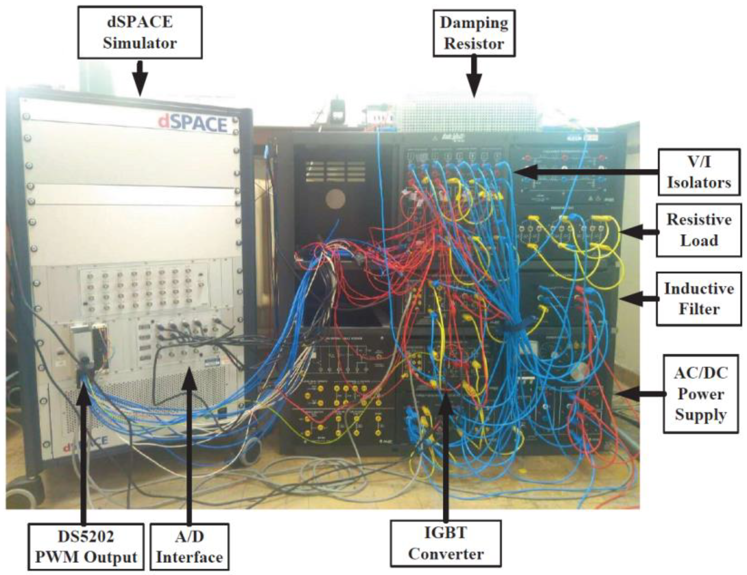
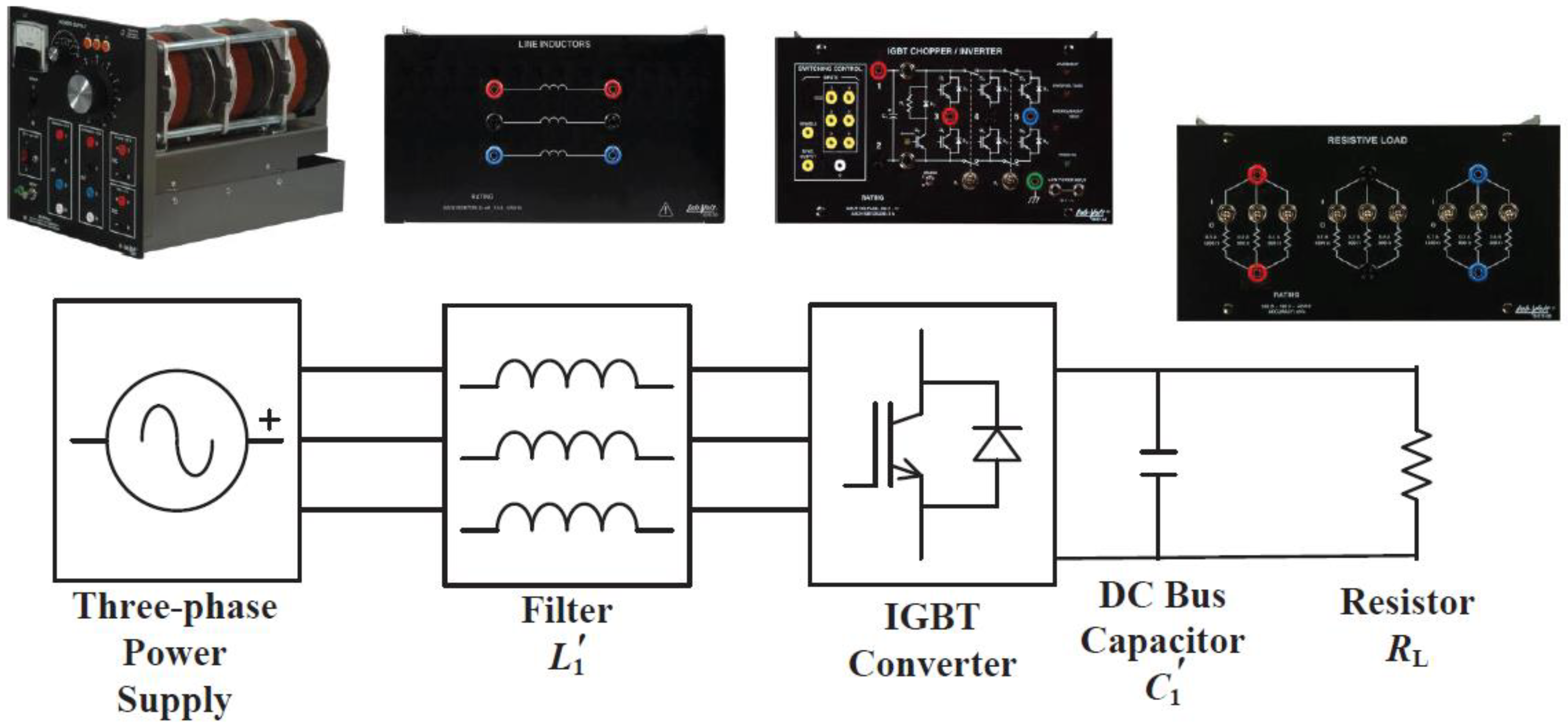
5.1. Experimental Platform

For the purpose of verifying the practicability of ONAC, a hardware experiment was carried out while the experimental platform is illustrated by Figure 5. A strong AC/DC power supply was used to provide stable three phase AC and DC voltages. The power supply was connected with the converter by an IGBT converter [27] with an inductive filter. IGBT converters can be driven by pulse width modulation (PWM) signals. Compared with the conventional PWM or sinusoidal pulse width modulation (SPWM) techniques, the space vector modulation (SVM) can increase 15% more of the maximum output voltage and reduce the switching times. The voltage/current isolators measured the voltages and currents, which were then sent to the dSPACE simulator through analogue/digital (A/D) blocks [28].

The dSPACE simulator had quad-core AMD (advanced micro devices) processors (DS1104) and operated with DS5202 ACMC board, which was capable of generating high-frequency PWM [29] signals and providing high-speed A/D interfaces. The IGBT converter, inductive filter, voltage/current isolators, and AC/DC power supply were all from the Lab-Volt company, which provides various equipment with the user-friendly interfaces, accurate system parameters, and reliable hardware protections. The DC bus of the IGBT converter was protected by adopting a 100 Ω damping resistor with 1 kW rated power connected to the damping circuit built in to the IGBT converter to avoid potential damages caused by overvoltage or overcurrent in the DC bus. Finally,

Table 2. The error specification of quad-core AMD (advanced micro devices) processors (DS 1104) board [30].

Component Parameters	A/D Converter	D/A Converter
Offset error	±5 mV	±1 mV
Gain error	Multiplexed channels: ±0.25%	±0.1%
	Parallel channels: ±0.5%
Offset drift	40 μV/K	130 μV/K
Gain drift	25 ppm/K	25 ppm/K
Signal-to-noise ratio	Multiplexed channels: >80 dB	>80 dB
	Parallel channels: >65 dB

demonstrates the guaranteed measurement error of DS1104 board.

The controller was embedded in the dSPACE platform (dSPACE Inc., Paderborn, Germany) shown in Figure 5, which measured the DC voltage, reactive power, and active power as inputs. Then, the PWM signals were generated with various duty cycles as controller outputs to the IGBT converter. Furthermore, the sampling frequency f_s and the PWM frequency f_PWM with SVPWM are given in

Table 3. System parameters used in the experiment.

Rated Active Power	P0	300 W
Rated rms voltage	V0	30 V
Rated rms current	I0	10 A
Rated frequency	f0	50 Hz
Filter inductance	L1′, L2′	60 mH
PWM frequency	fPWM	2 kHz
Sampling frequency	fs	10 kHz
DC bus capacitance	C1′, C2′	1320 µF
Load resistance	RL	1200 Ω

. Here, sampling frequency was determined by the performance of industrial microprocessors of VSC, which usually ranges from 1 kHz to 3 kHz. Note that a lower sampling frequency might degrade the control precision while a higher sampling frequency might increase the computation burden. To make a trade-off between the control precision and computation burden, this paper adopted the median sampling frequency (2 kHz) to validate the controller implementation feasibility. MSSA was run 30 times and the optimal outcomes (the controller gains and observer gains leading to the lowest fitness function) were undertaken in ONAC. The parameters of the controller are provided in

Table 4. Optimized controller gains and observer gains tuned by MSSA.

Rectifier Controller
Controller gains	$k_{\mathrm{r}1}=40$	$k_{\mathrm{r}1}^{\prime }=400$	$k_{\mathrm{r}2}^{\prime }=40$
	$b_{\mathrm{r}10}=105$	$b_{\mathrm{r}20}=-3000$
Observer gains	${\alpha }_{\mathrm{r}1}=80$	${\alpha }_{\mathrm{r}2}=1600$	${\alpha }_{\mathrm{r}1}^{\prime }=120=120$
	${\alpha }_{\mathrm{r}2}^{\prime }=4800$	${\alpha }_{\mathrm{r}3}^{\prime }=6.4\times {10}^4$	ε = 0.1
Inverter controller
Controller gains	$k_{i1}=20$	$k_{i1}^{\prime }=20$	$b_{i10}=100$
	$b_{i20}=-100$
Observer gains	${\alpha }_{i1}=60$	${\alpha }_{i2}=80$	${\alpha }_{i1}^{\prime }=60$
	${\alpha }_{i2}^{\prime }=900$	ε = 0.1

, while the control inputs were limited as |u_di| ≤ 50 V and |u_qi| ≤ 50 V, i = 1,2, respectively. Based on SVPWM and ignoring the resistance in the steady state, the minimum DC voltage must satisfy the following inequality to ensure the converter is controllable and can work properly as [16]

$$V_{\mathrm{dc}i}\ge \sqrt{3}\sqrt{{(u_{\mathrm{sd}i}+\omega Liiqi)}^2+{(u_{\mathrm{sq}i}-\omega Li{i}_{\mathrm{d}i})}^2}$$

(37)

At last, the IGBT converter was used as the DC/AC converter, the antiparallel diodes were combined with the IGBT converters such that it could be operated as either a rectifier or an inverter.

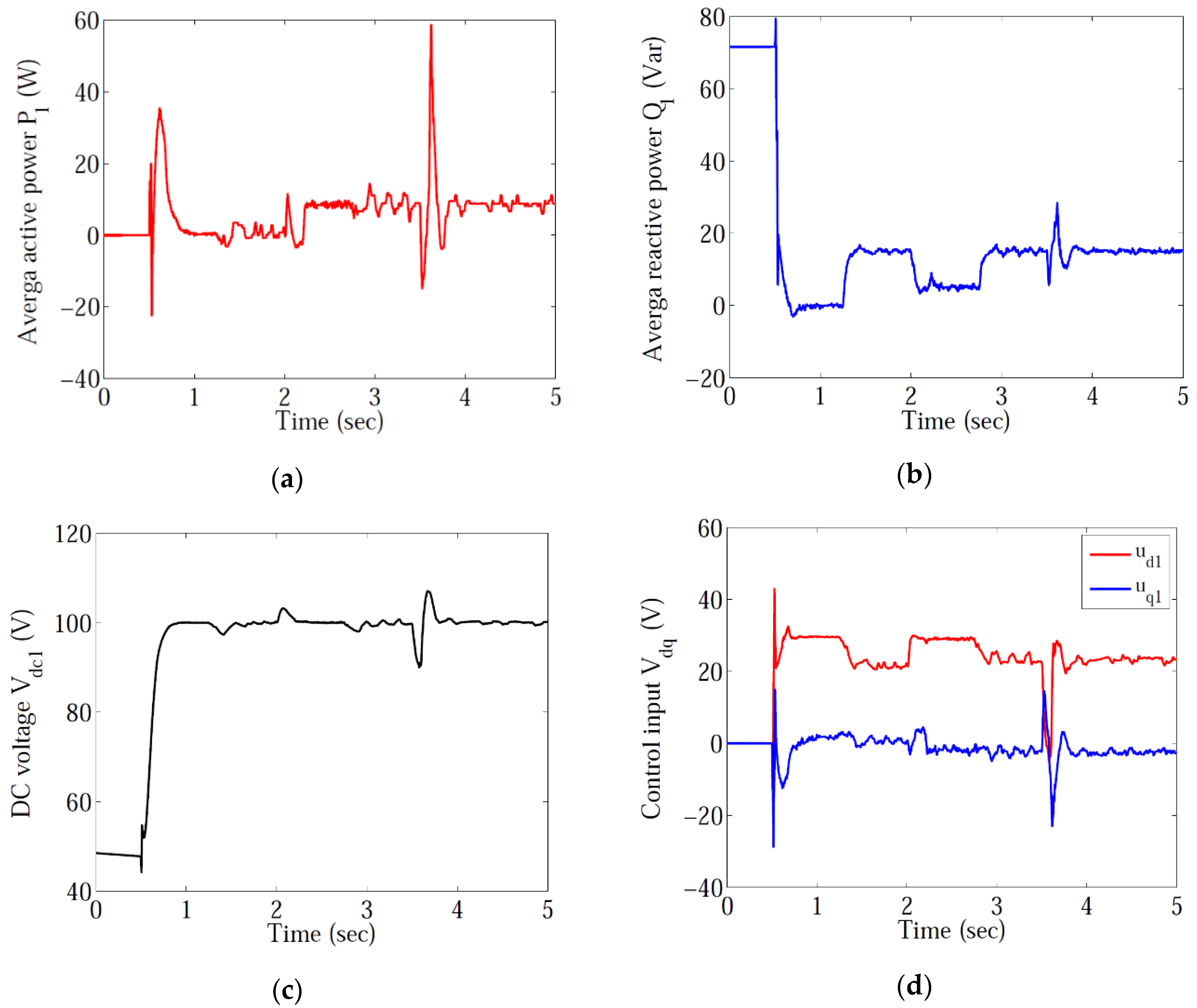
5.2. Rectifier Controller Experiment

The configuration of the rectifier controller experiment is illustrated by Figure 6, in which the DC bus was connected to a resistive load to achieve a specific evaluation of control performance when the active power flowed from the AC grid to the DC cable.

The effectiveness of the ONAC-based rectifier controller was tested at first, in which the initial DC voltage V_dc1 and reactive power Q₁ were adjusted to be 100 V and 0 Var, respectively. The DC voltage remained at 100 V for the whole period of the experiment. The reference of reactive power was set to be 15 Var, then dropped to 5 Var and was restored to 15 Var. After reactive power was stabilized at 15 Var, a resistive load R_L was connected to the DC bus given in Figure 6 to represent the DC cable. Then a 50% voltage drop of the AC grid occured to evaluate the system transient performance.

The experiment results are provided in Figure 7. It demonstrates that both the reactive power and DC voltage were rapidly regulated, while the DC voltage was able to be restored after the AC grid voltage drop occurred, which validates the effectiveness of the ONAC-based rectifier controller.

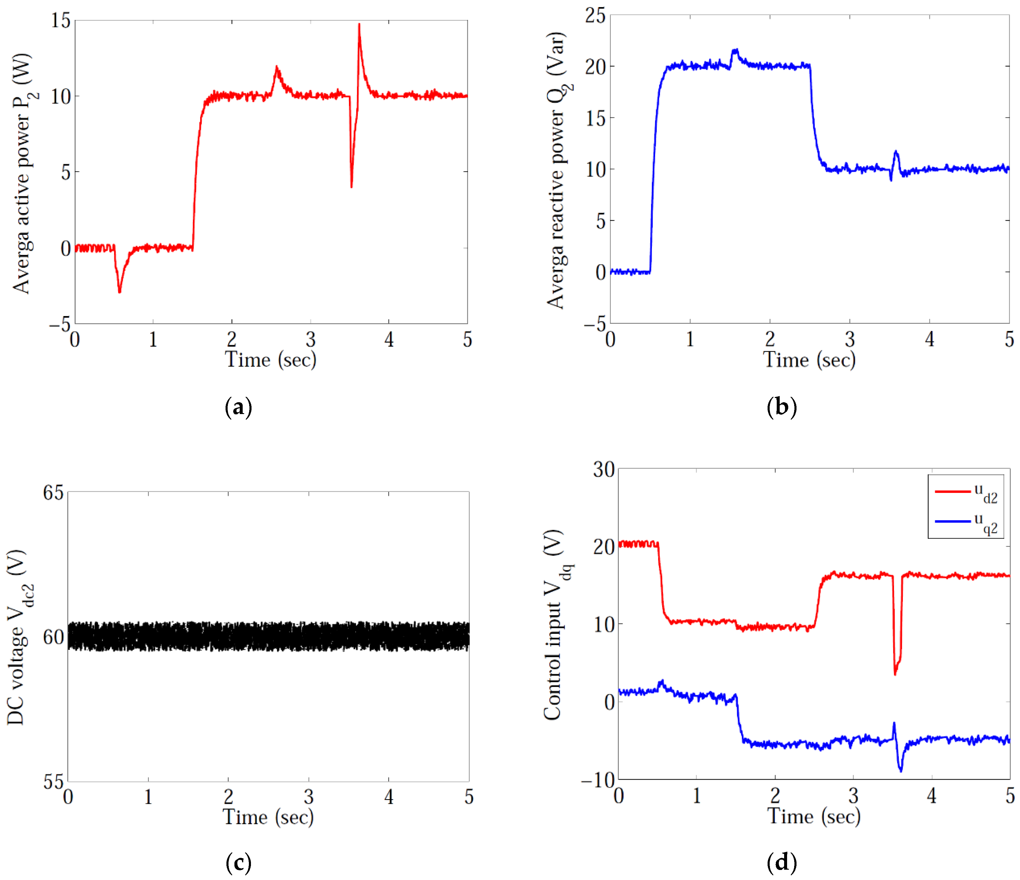
5.3. Inverter Controller Experiment

The configuration of the inverter controller experiment is shown in Figure 8, where a DC power supply was utilized to output a stable DC voltage (representing a constant DC voltage regulated by the rectifier controller) such that the IGBT converter could work properly.

The effectiveness of the ONAC-based inverter controller was then tested, the initial value of reactive power and active power were zero. The DC voltage V_dc2 was maintained at 60 V for the whole period of the experiment. The controller was activated to increase the reactive power Q₂ to be 20 Var at first; after reactive power Q₂ was stabilized the active power P₂ was increased to be 10 W, then the reactive power Q₂ was decreased to be 10 Var. At last a 33.3% voltage drop of the AC grid occurred to evaluate the system transient performance.

The experiment outcomes are given in Figure 9. Obviously, the reactive power and active power were able to be regulated independently, and the system could also be restored after the voltage drop, which verified the effectiveness of the ONAC-based inverter controller.

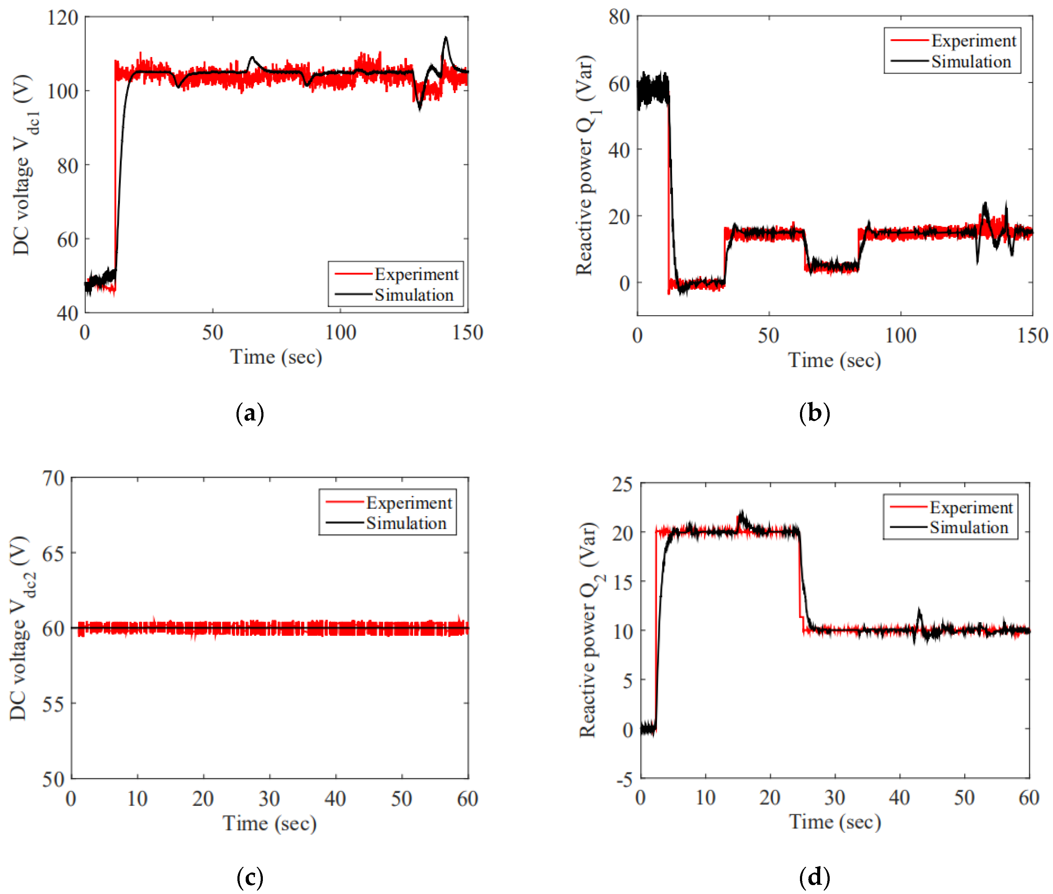
5.4. Set point Tracking

In order to evaluate the set point tracking performance of ONAC, both the simulation (set point curve) and experiment are compared in Figure 10. One can clearly observe that the experiment can closely track the set point, while their tiny difference resulted from the transmission delay of control signals or measurement noises during the experiment.

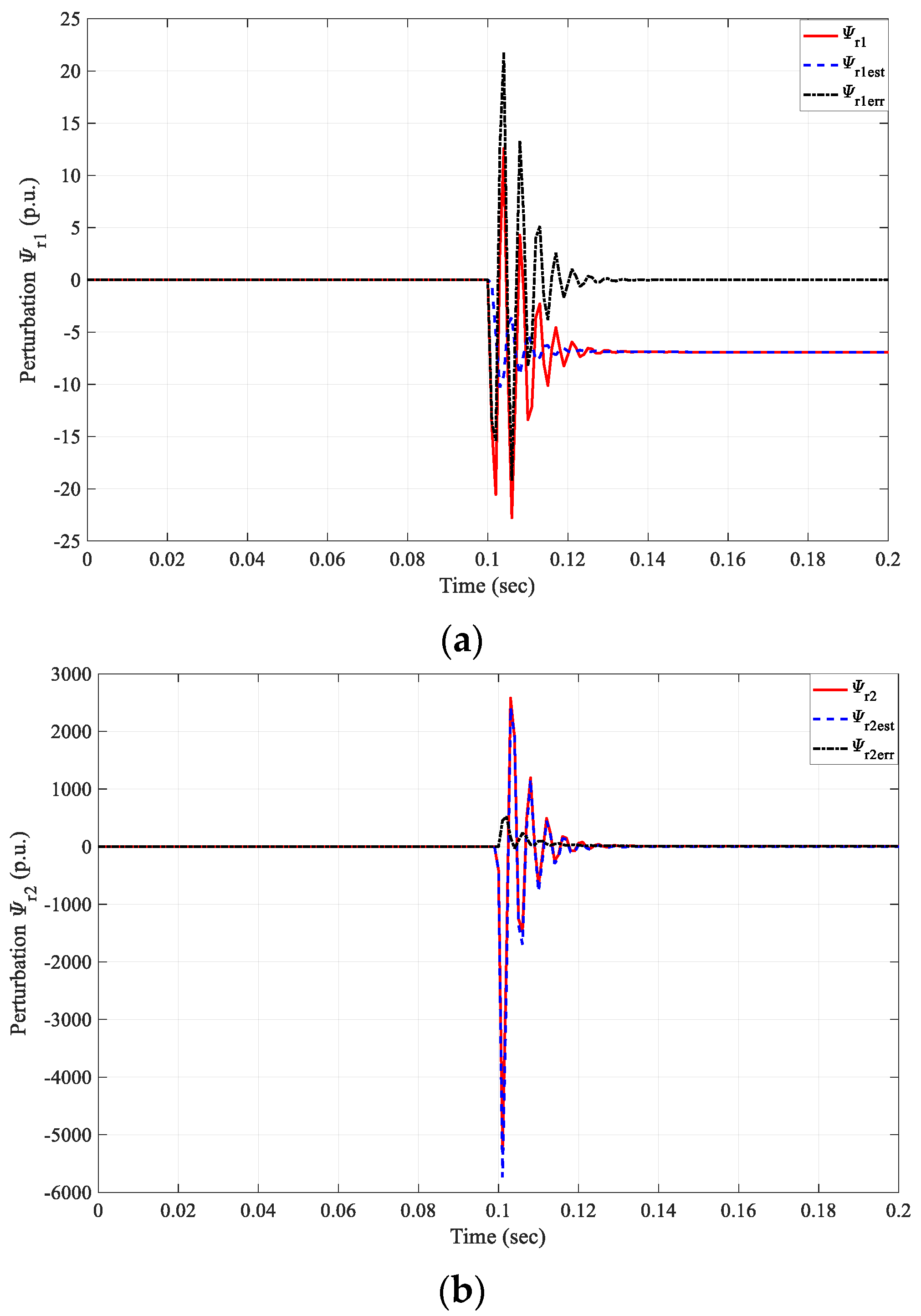
5.5. Disturbance Rejection

Disturbances are very common in many industrial processes which often have a malignant impact on the predesigned control performance of the studied system. As a result, disturbance rejection performance is a very crucial property for advanced controller design in industries [31,32,33]. This test aimed to evaluate the disturbance rejection performance of ONAC, while the perturbation estimation performance of HGPO under 20% voltage drop lasting for 15 ms (t = 0.1 s–0.115 s) of VSC under rectifier mode was recorded and illustrated in Figure 11. As shown in Figure 11, both perturbations ${\Psi }_{\mathrm{r}1}$ and ${\Psi }_{\mathrm{r}2}$ could be rapidly estimated by HGPO s under the voltage drop of VSC as the perturbation estimation error could be efficiently converged to 0. As a result, the disturbance was able to be effectively rejected as its real-time estimate could be rapidly obtained and then fully compensated by ONAC. Here, only the rectifier results are provided as it involved both the second-order HGPO (Figure 11a) and third-order HGPO (Figure 11b), while similar results could be found in inverter mode. Note that the transient relatively large variation of perturbation when the disturbance occurred was due to the high gains used in HGPO.

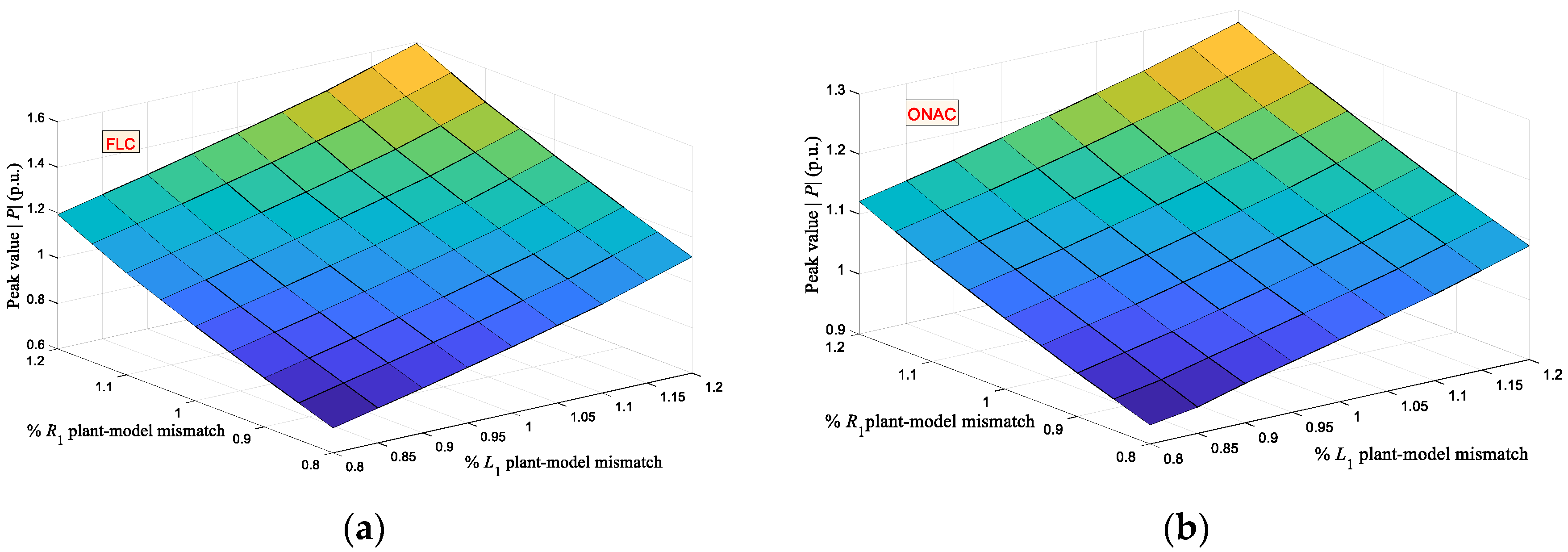
5.6. Robustness to Parameter Uncertainties

Lastly, the robustness to parameter uncertainties was investigated in this section. Here, a series of plant model mismatches of equivalent resistance R₁ and inductance L₁ within ±20% variation around their nominal value were undertaken. Then, a 50% voltage drop lasting 100 ms at VSC was applied, in which the peak value of output power |P| was recorded. Figure 12 shows that the variation of peak value of active power |P| obtained by FLC [10] and ONAC were 73.4% and 26.5%, which clearly demonstrated that ONAC provided the highest robustness against VSC parameter uncertainties thanks to the real-time compensation of perturbation, while FLC was vulnerable to parameter uncertainties as it required an accurate VSC system model.

6. Conclusions

This paper designed an ONAC-based rectifier controller and ONAC based inverter controller. It can provide significant robustness as various modelling uncertainties were aggregated into a perturbation, which was rapidly evaluated by HGPO and then compensated for by the proposed controller. Besides, ONAC merely needs the active power and reactive power, as well as DC voltage need to be measured, while a precise VSC system model is not required, thus the proposed controller can be readily implemented in practice. Moreover, the controller gains and observer gains are optimally tuned by an emerging and promising biology based metaheuristic algorithm called MSSA, which can effectively achieve an appropriate trade-off between global exploration and local exploitation, thus a satisfactory control performance and perturbation estimation performance could be guaranteed. Finally, for the sake of verifying the practicability of the proposed controller, a hardware experiment utilizing dSPACE platform was undertaken. The experiment results showed that ONAC could achieve satisfactory control performance.

Future studies will apply ONAC-based VSC on renewable energy systems, e.g., PV inverter, wind energy conversion systems, as well as electric energy storage systems.

References

1. He, Y.Q.; Chen, Y.H.; Yang, Z.Q.; He, H.B.; Li, L. A review on the influence of intelligent power consumption technologies on the utilization rate of distribution network equipment. Prot. Control Mod. Power Syst. 2018, 3, 183–193. [Google Scholar] [CrossRef]
2. Ruan, S.Y.; Li, G.J.; Jiao, X.H.; Sun, Y.Z.; Lie, T. Adaptive control design for VSC-HVDC systems based on backstepping method. Electr. Power Syst. Res. 2007, 77, 559–565. [Google Scholar] [CrossRef]
3. Nguyen, T.T. A rotor-sync signal-based control system of a doubly-fed induction generator in the shaft generation of a ship. Processes 2019, 7, 188. [Google Scholar] [CrossRef]
4. Li, J.H.; Wang, S.; Ye, L.; Fang, J.K. A coordinated dispatch method with pumped-storage and battery-storage for compensating the variation of wind power. Prot. Control Mod. Power Syst. 2018, 3, 21–34. [Google Scholar] [CrossRef]
5. Han, P.P.; Fan, G.J.; Sun, W.Z.; Shi, B.L.; Zhang, X.A. Research on identification of LVRT characteristics of photovoltaic inverters based on data testing and PSO algorithm. Processes 2019, 7, 250. [Google Scholar] [CrossRef]
6. Yang, B.; Zhang, X.S.; Yu, T.; Shu, H.C.; Fang, Z.H. Grouped grey wolf optimizer for maximum power point tracking of doubly-fed induction generator based wind turbine. Energy Convers. Manag. 2017, 133, 427–443. [Google Scholar] [CrossRef]
7. Yang, B.; Jiang, L.; Wang, L.; Yao, W.; Wu, Q.H. Nonlinear maximum power point tracking control and modal analysis of DFIG based wind turbine. Int. J. Electr. Power Energy Syst. 2016, 74, 429–436. [Google Scholar] [CrossRef] [Green Version]
8. Dash, P.K.; Patnaik, R.K.; Mishra, S.P. Adaptive fractional integral terminal sliding mode power control of UPFC in DFIG wind farm penetrated multimachine power system. Prot. Control Mod. Power Syst. 2018, 3, 79–92. [Google Scholar] [CrossRef]
9. Ruan, S.Y.; Li, G.J.; Peng, L.; Sun, Y.Z.; Lie, T.T. A nonlinear control for enhancing HVDC light transmission system stability. Int. J. Electr. Power Energy Syst. 2007, 29, 565–570. [Google Scholar] [CrossRef]
10. Moharana, A.; Dash, P.K. Input-output linearization and robust sliding-mode controller for the VSC-HVDC transmission link. IEEE Trans. Power Deliv. 2010, 25, 1952–1961. [Google Scholar] [CrossRef]
11. Li, S.; Haskew, T.A.; Xu, L. Control of HVDC light system using conventional and direct current vector control approaches. IEEE Trans. Power Electron. 2010, 25, 3106–3118. [Google Scholar]
12. Yang, B.; Yu, T.; Shu, H.C.; Zhang, Y.M.; Chen, J.; Sang, Y.Y.; Jiang, L. Passivity-based sliding-mode control design for optimal power extraction of a PMSG based variable speed wind turbine. Renew. Energy 2018, 119, 577–589. [Google Scholar] [CrossRef]
13. Yang, B.; Yu, T.; Shu, H.C.; Dong, J.; Jiang, L. Robust sliding-mode control of wind energy conversion systems for optimal power extraction via nonlinear perturbation observers. Appl. Energy 2018, 210, 711–723. [Google Scholar] [CrossRef]
14. Tang, R.L.; Wu, Z.; Fang, Y.J. On figuration of marine photovoltaic system and its MPPT using model predictive control. Sol. Energy 2017, 158, 995–1005. [Google Scholar] [CrossRef]
15. Mohomad, H.; Saleh, S.A.M.; Chang, L. Disturbance estimator-based predictive current controller for single-phase interconnected PV systems. IEEE Trans. Ind. Appl. 2017, 53, 4201–4209. [Google Scholar] [CrossRef]
16. Yao, J.; Jiao, Z.; Ma, D. Extended-state-observer-based output feedback nonlinear robust control of hydraulic systems with backstepping. IEEE Trans. Power Electron. 2014, 61, 6285–6293. [Google Scholar] [CrossRef]
17. Xue, W.; Bai, W.; Yang, S.; Song, K.; Huang, Y.; Xie, H. Adrc with adaptive extended state observer and its application to air–fuel ratio control in gasoline engines. IEEE Trans. Ind. Electron. 2015, 62, 5847–5857. [Google Scholar] [CrossRef]
18. Cui, R.X.; Chen, L.P.; Yang, C.G.; Chen, M. Correction to extended state observer-based integral sliding mode control for an underwater robot with unknown disturbances and uncertain nonlinearities. IEEE Trans. Ind. Electron. 2017, 64, 6785–6795. [Google Scholar] [CrossRef]
19. Wu, Q.H.; Jiang, L.; Wen, J.Y. Decentralized adaptive control of interconnected non-linear systems using high gain observer. Int. J. Control 2004, 77, 703–712. [Google Scholar] [CrossRef]
20. Jiang, L.; Wu, Q.H.; Wen, J.Y. Decentralized nonlinear adaptive control for multi-machine power systems via high-gain perturbation observer. IEEE Trans. Circuits Syst. I Regul. Pap. 2004, 51, 2052–2059. [Google Scholar] [CrossRef]
21. Chen, J.; Jiang, L.; Wei, Y.; Wu, Q.H. Perturbation estimation based nonlinear adaptive control of a full-rated converter wind turbine for fault ride-through capability enhancement. IEEE Trans. Power Syst. 2014, 29, 2733–2743. [Google Scholar] [CrossRef]
22. Yang, B.; Zhong, L.E.; Yu, T.; Li, H.F.; Zhang, X.S.; Shu, H.C.; Sang, Y.Y.; Jiang, L. Novel bio-inspired memetic salp mswarm algorithm and application to MPPT for PV systems considering partial shading condition. J. Clean. Prod. 2019, 215, 1203–1222. [Google Scholar] [CrossRef]
23. Eusuff, M.; Lansey, K.; Pasha, F. Shuffled frog-leaping algorithm: A memetic meta-heuristic for discrete optimization. Eng. Optim. 2006, 38, 129–154. [Google Scholar] [CrossRef]
24. Mirjalili, S.; Gandomi, A.H.; Mirjalili, S.Z.; Saremi, S.; Faris, H.; Mirjalili, S.M. Salp swarm algorithm: A bio-inspired optimizer for engineering design problems. Adv. Eng. Softw. 2017, 114, 163–191. [Google Scholar] [CrossRef]
25. Eusuff, M.M.; Lansey, K.E. Optimization of water distribution network design using the shuffled frog leaping algorithm. J. Water Resour. Plan. Manag. 2015, 129, 210–225. [Google Scholar] [CrossRef]
26. Bharatiraja, C.; Jeevananthan, S.; Latha, R. FPGA based practical implementation of NPC-MLI with SVPWM for an autonomous operation PV system with capacitor balancing. Int. J. Electr. Power Energy Syst. 2014, 61, 489–509. [Google Scholar] [CrossRef]
27. Xia, Y.; Gou, B.; Xu, Y. A new ensemble-based classifier for IGBT open-circuit fault diagnosis in three-phase PWM converter. Prot. Control Mod. Power Syst. 2018, 3, 364–372. [Google Scholar] [CrossRef]
28. Smith, M. DSpace: An Open Source Dynamic Digital Repository. 2003. Available online: https://dspace.mit.edu/handle/1721.1/29465 (accessed on 9 July 2019).
29. Holmes, D.G.; Lipo, T.A. Pulse Width Modulation for Power Converters: Principles and Practice; John Wiley & Sons: Hoboken, NJ, USA, 2003. [Google Scholar]
30. Single-Board Hardware /DS1104 R&D Controller Board. Available online: https://www.dspace.com/shared/data/pdf/2018/dSPACE_DS1104_Catalog2018.pdf (accessed on 25 May 2019).
31. Gao, Z.; Saxen, H.; Gao, C. Special Section on Data-Driven Approaches for Complex Industrial Systems. IEEE Trans. Ind. Inform. 2013, 9, 2210–2212. [Google Scholar] [CrossRef]
32. Gao, Z.; Nguang, S.K.; Kong, D.X. Advances in Modelling, monitoring, and control for complex industrial systems. Complexity 2019, 2019. [Google Scholar] [CrossRef]
33. Cao, H.Z.; Yu, T.; Zhang, X.S.; Yang, B.; Wu, Y.X. Reactive power optimization of large-scale power systems: A transfer bees optimizer application. Processes 2019, 7, 321. [Google Scholar] [CrossRef]
Figure 1. The structure of voltage source converters (VSC).
Processes 07 00490 g001
Figure 2. Optimization framework of memetic salp swarm algorithm (MSSA).
Processes 07 00490 g002
Figure 3. The overall optimal nonlinear adaptive control (ONAC)-based control framework of rectifier.
Processes 07 00490 g003
Figure 4. The overall ONAC-based control framework of inverter.
Processes 07 00490 g004
Figure 5. The experimental platform based on the dSPACE platform.
Processes 07 00490 g005
Figure 6. The configuration of the rectifier controller experiment.
Processes 07 00490 g006
Figure 7. System responses obtained in the rectifier controller experiment: (a) Average active power P 1 ; (b) average active power Q 1 ; (c) DC voltage V dc 1 ; (d) control input V dq .
Processes 07 00490 g007
Figure 8. The configuration of the inverter controller experiment.
Processes 07 00490 g008
Figure 9. System responses obtained in the inverter controller experiment. (a) Average active power P 2 ; (b) average active power Q 2 ; (c) DC voltage V dc 2 ; (d) control input V dq .
Processes 07 00490 g009
Figure 10. System responses obtained under set point tracking. (a) DC voltage V dc 1 of rectifier; (b) average reactive power Q 1 of rectifier; (c) DC voltage V dc 2 of inverter; (d) average reactive power Q 2 of inverter.
Processes 07 00490 g010
Figure 11. Disturbance rejection performance obtained under 20% voltage drop of rectifier. (a) Perturbation Ψ r 1 and (b) perturbation Ψ r 2 .
Processes 07 00490 g011
Figure 12. Peak value of active power |P| obtained under a 50% voltage drop lasting 100 ms at VSC with 20% variation of the equivalent resistance R1 and inductance L1 of FLC and ONAC. (a) FLC and (b) ONAC.
Processes 07 00490 g012