Global Sensitivity Analysis of a Spray Drying Process

Abstract

Spray drying is a key unit operation used to achieve particulate products of required properties. Despite its widespread use, the product and process design, as well as the process control remain highly empirical and depend on trial and error experiments. Studying the effect of operational parameters experimentally is tedious, time consuming, and expensive. In this paper, we carry out a model-based global sensitivity analysis (GSA) of the process. Such an exercise allows us to quantify the impact of different process parameters, many of which interact with each other, on the product properties and conditions that have an impact on the functionality of the final drug product. Moreover, classical sensitivity analysis using the Sobol-based sensitivity indices was supplemented by a polynomial chaos-based sensitivity analysis, which proved to be an efficient method to reduce the computational cost of the GSA. The results obtained demonstrate the different response dependencies of the studied variables, which helps to identify possible control strategies that can result in major robustness for the spray drying process.

1. Introduction

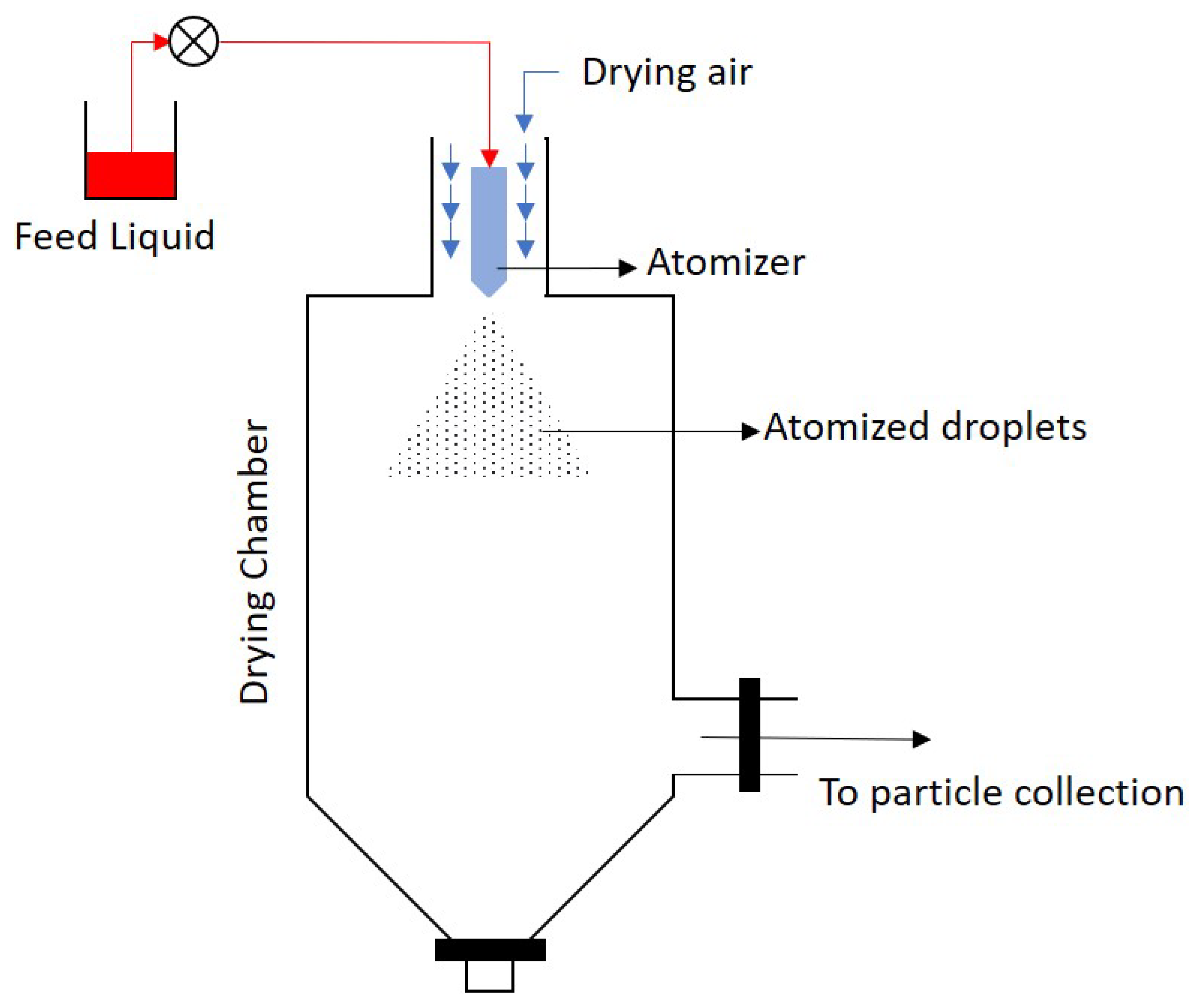
Spray drying is a widely-used unit operation in the production of high-value-added products in the food, fertilizers, chemical, and pharmaceutical industries [1,2,3,4]. Its application ranges from the production of milk and other diary products, to the very complex formulations of composite materials used in medicines, to biological products for which few other drying technologies are feasible. Spray drying is a cost-efficient, continuous, and relatively easy to operate process [5]. A typical spray dryer, as shown in Figure 1, consists of two sections, an atomization section and a drying section. The atomizer disperses the liquid mixture into small droplets, which then fall into the drying chamber. Small droplets dispersed in a hot gas medium offer large surface areas for mass and energy transfer, while guaranteeing short exposure of the product to high temperatures [6,7]. The dried product is then collected using an array of cyclones and filters. Spray drying allows a more specific functional design of products. It provides high flexibility on the input mixture because the liquid feed can be provided in various forms, e.g., solutions, emulsions, or suspensions. The nature of the particulate product ranges from pure substances, solid blends, to composite materials, and viable biological components. With proper tuning, spray drying offers relatively narrow particle size distributions in the range between nano- to micro-sized particles [8,9,10], and good control over other particle properties like residual solvent content, morphology, and density. The major tuning parameters include the flow rate and temperature of the feed and drying gas; concentration, surface tension, viscosity, and density of the liquid feed; flow configuration; and atomizer geometry. Any variations in these process conditions or the input feed properties will thus affect the downstream properties.

The continuous push from regulatory agencies, the tightening quality requirements, and the increase in the number of specialized drug products drive the research on spray drying towards the development of model-based approaches that replace the traditional empirical practices. Similar to many other unit operations that handle particulate systems, the setup of large-scale spray drying operations remains highly empirical [1]. Due to the complexity of the multiphase system involved, the process conditions for spray drying are traditionally determined by trial and error experiments. This approach normally involves large investments in time and money to determine those process conditions that result in a dried product with the desired properties. In the pharmaceutical industry, the quality by design paradigm (QbD) has already pushed for a more systematic view of the exploitation of the experimental knowledge [11]. Applying QbD to the spray drying process entails: (i) determination of powder properties, which are critical quality attributes (CQAs) based on the impact they have on the performance of the drug product, (ii) identification of the critical process parameters (CPPs) and input material attributes (CMAs) that affect the CQAs, and (iii) establishment of a design space and control strategy in terms of CPPs and CMAs that can guarantee the CQAs’ requirements.

Within this context, this work evaluates the use of global sensitivity analysis (GSA) as a model-based approach to apply the principles of QbD to the spray drying process. This approach bridges the research drive towards model-based methods for spray drying and the goals of QbD in the pharmaceutical industry. Previous research in these lines has focused on developing models for spray drying [1,12,13,14,15,16] or on QbD for spray drying using the design of experiments and defining the design space based on statistical analysis of the experimental data [17,18,19,20]. In this work, the focus is put first on the evaluation of the methods to apply GSA to the spray drying process, followed by the critical analysis of the results to demonstrate its potential to exploit the knowledge of the system contained in the model. GSA offers a structured approach to identify, quantify, and rank the influences of the CPPs and CMAs on the CQAs.

Several models have been developed in the past for the spray drying process. The level of detail and associated complexity of these varies from considering one dimensional differential equations [12,13] to complex partial differential equations, which aim to capture gradients in more multiple dimensions [15]. CFD simulations show the complex flow patterns that are developed inside the drying chamber due to the geometry of the chamber, velocity and pressure gradients in the gas, as well as the size distribution of the particles [16]. Studies on atomization generally consider empirical equations to model specific types of nozzles. Since the aim of this work is to demonstrate the power of GSA to capture the global relation between variables and the mean responses of the CQAs, a validated one-dimensional system of differential equations is chosen to describe the spray drying process [1]. This model is described in Section 2.1. Additionally, two different atomization nozzle configurations are considered to evaluate the differences induced in the process and the product. The pneumatic and the pressure nozzle considered are discussed in Section 2.3.

A traditional approach to GSA is the use of Sobol sensitivity indices, which result from an analysis of variance on the system [21]. This method is discussed in Section 2.2.1. An analytical solution to partial variances is almost impossible for complex mathematical models, and typically, approximations based on (quasi) Monte Carlo sampling are used. The current best practices to calculate the sensitivity indices make use of Saltelli’s approach with a sufficient number of quasi-random samples [22,23]. However, a large number of model evaluations for complex models lead to exorbitant computational times. More computationally-efficient methods for the approximation of sensitivity indices are based on surrogate meta-models. These approaches have already been investigated for the GSA of (bio)chemical processes [24]. In this work, polynomial chaos expansion (PCE) is used as a way to construct the meta-model for spray drying and reduce the computational burden for the GSA [25,26,27]. PCE is based on the probabilistic projection of the model output on the basis of orthogonal stochastic polynomials. In this work, arbitrary or data-driven is investigated, as it does not depend on an assumption of any specific probability distribution functions (PDF) for the inputs. To assess the PCE-based sensitivity indices, we assume that the indices based on Saltelli’s approach are true iff the number of samples is large enough. The question of the size of the sample set is discussed in Section 3.1. In the same section, the sensitivity indices calculated using the PCE are then compared to the Saltelli approximations.

The results obtained are discussed in Section 3.2 and Section 3.3. Two main aspects are reviewed based on these results. (i) The validity of GSA using arbitrary or data-driven polynomial chaos expansions (aPCE) is evaluated with respect to the indices computed from the comprehensive variance analysis based on Saltelli’s method. (ii) A critical discussion is provided on the results of the GSA for the spray drying process.

2. Materials and Methods

2.1. Spray Drying Model

Considering the co-current gas flow spray dryer, the process proceeds in the following stages. First, the liquid feed is atomized using special nozzles, and the droplets enter the drying chamber. The solvent is then evaporated from the droplets by the drying gas fed to the chamber. At one point along the drying chamber, the droplets transition to solid particles, which then need to be separated from the drying gas. In this paper, the atomization section is modeled independently of the drying section. The spray drying model developed in [1] was used for the study. The spray dryer is modelled axially, ignoring any radial effects under a number of other simplifying assumptions.

For the solids, the humidity $\left(W_p\right)$ in the droplet/particle follows Equation (1)

$$\begin{array}{cc}\hfill \frac{d{W}_p}{dz}& =-\frac{\pi d_p{\dot{m}}_v}{v_p{m}_s},W_p(z=0)=W_{p0}\hfill \end{array}$$

(1)

where z is the axial distance, $v_p$ and $d_p$ are the particle velocity and diameter, $m_s$ is the mass of solids in the droplet (estimated from the initial liquid concentration), and ${\dot{m}}_v$ is the rate of evaporation. The particle humidity evolves until an equilibrium moisture content is reached. After this point, it stabilizes, and the evaporation rate drops to zero.

A particle/droplet in the spray dryer goes through various stages of drying. Initially, as the rate of evaporation is balanced by the rate of moisture transfer from the center of the particle to the surface, the droplet shrinks in size, while its density increases. Further down the chamber, a critical moisture content is reached where the droplet transitions to being a “wet particle”, and the size of the particle remains constant. The transition of the wet particle to a dry particle is limited by the rate of moisture being wicked to the surface of the particle. Once the equilibrium moisture content is reached, the particle stops drying, and its density $\left({\rho }_p\right)$ and size $\left(d_p\right)$ remain constant. Cotabarren et al. [1] modeled the process as follows.

When $W_p\ge W_{pc}$,

$$\begin{array}{ccc}\hfill \frac{d{d}_p}{dz}& =\frac{d_{p0}{\dot{m}}_v\pi d_p^2}{3m_s{v}_p}{\left(\frac{{\rho }_{p0}-{\rho }_w}{{\rho }_p-{\rho }_w}\right)}^{-\frac{2}{3}}\left(\frac{{\rho }_{p0}-{\rho }_w}{{({\rho }_p-{\rho }_w)}^2}\right)\left(\frac{1-\frac{{\rho }_s}{{\rho }_w}}{{(1+\frac{{\rho }_s}{{\rho }_w}{W}_p)}^2}\right),\hfill & d_p(z=0)=d_{p0}\hfill \end{array}$$

(2)

$$\begin{array}{ccc}\hfill \frac{d{\rho }_p}{dz}& =-\frac{{\dot{m}}_v\pi d_p^2{\rho }_s}{m_s{v}_p}\frac{1-\frac{{\rho }_s}{{\rho }_w}}{{(1+\frac{rh{o}_s}{rh{o}_w}{W}_p)}^2},\hfill & {\rho }_p(z=0)={\rho }_{p0}\hfill \end{array}$$

(3)

when $W_{peq}\le W_p<W_{pc}$:

$$\begin{array}{cc}\hfill \frac{d{d}_p}{dz}& =0\hfill \end{array}$$

(4)

$$\begin{array}{cc}\hfill \frac{d{\rho }_p}{dz}& =-\frac{6{\dot{m}}_v}{d_p{v}_p}\hfill \end{array}$$

(5)

and when $W_p<W_{peq}$,

$$\begin{array}{cc}\hfill \frac{d{\rho }_p}{dz}& =0\hfill \end{array}$$

(6)

The particle velocity is modeled by balancing the gravity with the drag forces acting on the particles.

$$\begin{array}{c}\hfill \frac{d{v}_p}{dz}=g{\left(\frac{{\rho }_p-{\rho }_a}{{\rho }_p{v}_p}\right)}^{-\frac{3}{4}}-\frac{3C_D{\rho }_a}{4d_p{\rho }_p{v}_p}(v_a-v_p)|v_a-v_p|\end{array}$$

(7)

The rate of evaporation is described as a function of relative humidity of the gas and its saturation moisture content at the particle surface temperature [28].

$$\begin{array}{cc}\hfill {\dot{m}}_v& =\beta (Y_{sat}-Y_b)\hfill \end{array}$$

(8)

$$\begin{array}{cc}\hfill Y_{sat}& =\frac{P_v{\tilde{M}}_w}{(P-P_v){\tilde{M}}_a}\hfill \end{array}$$

(9)

The vapor pressure $P_v$ was calculated using Antoine’s equations. Pis the atmospheric pressure, and ${\tilde{M}}_{\{a,w\}}$ is the molecular weight of the gas (air) and solvent (water). The mass transfer coefficient is estimated as:

$$\begin{array}{c}\hfill \beta =\frac{\alpha {\rho }_a{\mathcal{D}}_{eff}}{k_a}\end{array}$$

(10)

The heat transfer coefficient $\alpha$ is estimated using empirical formulation [28,29]

$$\begin{array}{c}\hfill Nu=2+0.6R{e}^{0.5}P{r}^{0.33}\end{array}$$

(11)

where $Nu$ is the Nusselt number, $Re$ the particle Reynolds number, and $Pr$ the Prandtl number. The energy balance on a single particle/droplet is given by:

$$\begin{array}{c}\hfill \frac{d{T}_p}{dz}=\frac{\pi d_p^2[\alpha (T_a-T_p)-{\dot{m}}_v\Delta H_{ev}]}{v_p{m}_s(c_{p,s}+W_p{c}_{p,w})},T_p(z=0)=T_{p0}\end{array}$$

(12)

where $T_p$ is the particle temperature and $\Delta H_{ev}$ is the evaporation enthalpy of water.

The gas phase balances consider the total number of droplets, $N_t$, which is estimated as:

$$\begin{array}{c}\hfill N_t=\frac{{\dot{M}}_l}{V_{p0}{\rho }_{p0}}\end{array}$$

(13)

where ${\dot{M}}_l$ is the liquid mass flowing though the atomization nozzles and $V_{p0}$ is the initial droplet volume.

The gas moisture $\left(Y_b\right)$ balance is written as:

$$\begin{array}{c}\hfill \frac{d{Y}_b}{dz}=N_t\frac{{\dot{m}}_v\pi d_p^2}{{\dot{M}}_a{v}_p},Y_b(z=0)=Y_{b0}\end{array}$$

(14)

The drying gas temperature $\left(T_a\right)$ evolves as follows:

$$\begin{array}{c}\hfill \frac{d{T}_a}{dz}=-\frac{N_t\pi d_p^2({\dot{m}}_v{c}_{p,v}+\alpha )(T_a-T_p)}{v_p{\dot{M}}_a(c_{p,a}+X_b{c}_{p,v})}+\frac{U(T_a-T_{amb})\pi D_c}{{\dot{M}}_a(c_{p,a}+X_b{c}_{p,v})},T_a(z=0)=T_{a0}\end{array}$$

(15)

Further details on the model can be found in [1]. The limits of the empirical relations used to calculate the dimensionless numbers (i.e., Re, Pr, Nu) and the mass and energy transfer coefficients are valid for the wide range of possible conditions observed in a spray drying chamber. These relations were tested in [29], in the range $0\le Re\le 200$ and for gas temperatures up to 220 °C.

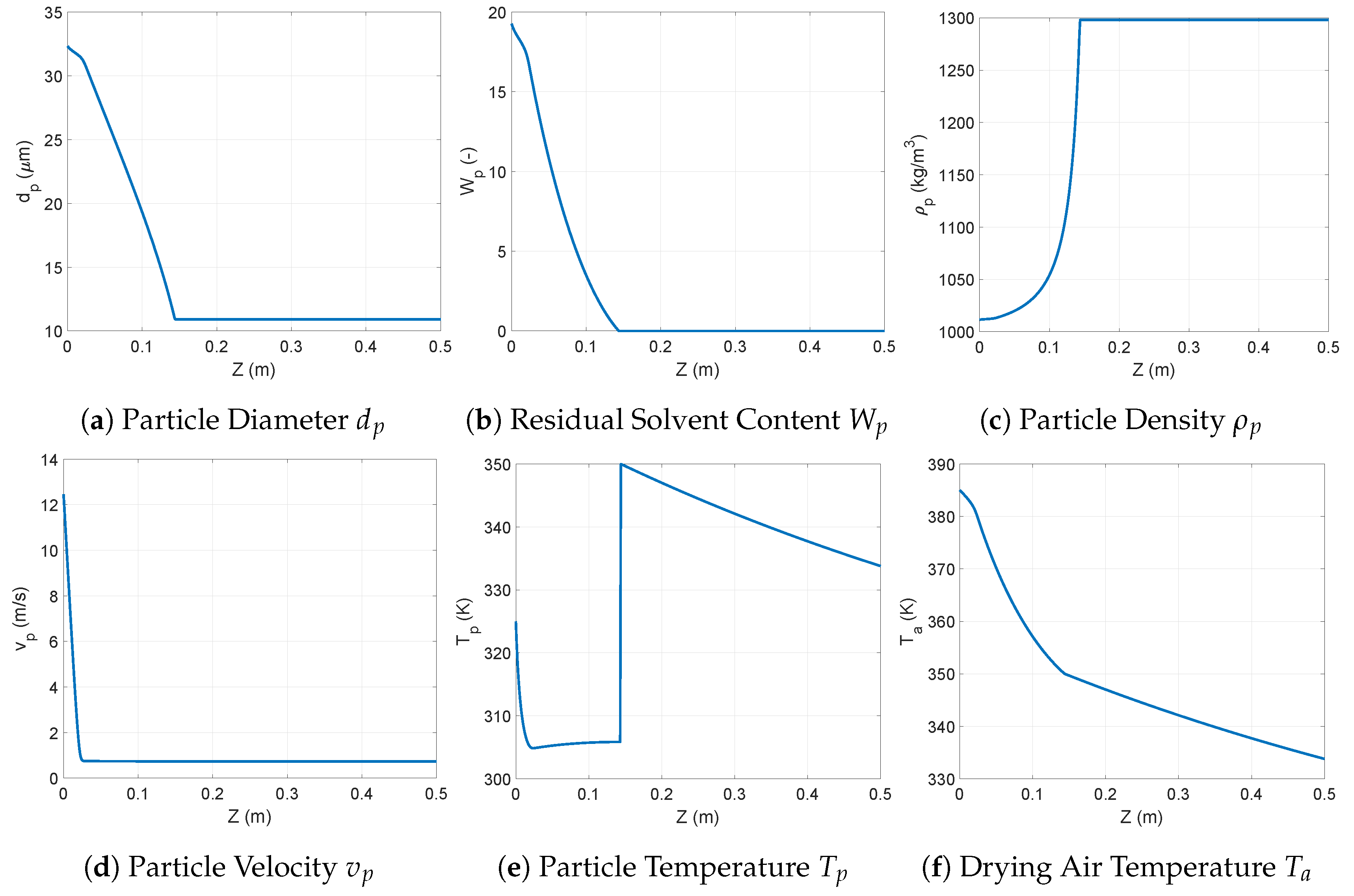
A typical spray drying profile obtained through the solution of the above model is depicted in Figure 2. The profiles observed for all variables illustrate that most of the changes occur in the first part of the drying chamber (i.e., $Z<\sim 0.14\left(\mathrm{m}\right)$); this is before the equilibrium humidity is reached. After this point, most of the variables display a steady value. Only the temperatures continue to change due to the heat transfer through the exterior wall of the drying chamber. In this part, the temperature of the gas and of the particle are equal. In the section before the equilibrium point, the droplet/particle velocity determines two distinctive phases. At the very beginning, when the droplet velocity is significantly higher than that of the air (i.e., $Z<\sim 0.02\left(\mathrm{m}\right)$), the conditions for mass transfer are favored by the turbulence around the droplets, and therefore, a high evaporation rate of the solvent can be observed. This causes the temperature of the droplet to drop because energy is consumed for evaporation faster than it is transferred from the hot air. The rate of change in droplet size and humidity is also distinctive in this section. Once the droplets have reached terminal velocity, the rate of evaporation is controlled by the energy transferred from the hot air to the droplet, and so the temperature stabilizes around a given value. In this section, the particle size and humidity continue to decrease. This phase ends when the particle has reached the equilibrium humidity. On the one hand, this stops the evaporation, reaching the final particle size, humidity, and density. The temperature, on the other hand, rises very quickly to reach equilibrium with the air temperature.

2.2. Global Sensitivity Analysis

The aim of sensitivity analysis (SA) is to study the variation in the outputs due to a variation in the inputs. Local SA methods typically consider only one input and one output (e.g., one-at-a-time analysis) and are limited to small variations around the nominal operating point. Global sensitivity methods (GSA) focus on output variations over a larger range of inputs, which are considered individually (first order effects) and together (higher order/interaction effects). A classical variance-based GSA method is the method using Sobol’s sensitivity indices [21]. The sensitivity indices are obtained via the ANOVA decomposition (Sobol decomposition) of the model outputs. Here, we discuss a brief theory of variance based GSA followed by practical methods to estimate these indices.

2.2.1. Variance-Based Sensitivity Analysis

Consider an d-dimensional input parameter vector $\mathbf{\theta }$ with a parameter space ${\Omega }_d$. The parameters are independent identically distributed (iid) random variables with a probability density function (PDF) $p\left(\mathbf{\theta }\right)$. Since the parameters are iid, $p\left(\mathbf{\theta }\right)={\prod }_{i}p\left({\theta }_i\right)$. A physical model $y=f\left(\mathbf{\theta }\right)$ describes the response of a physical system. Note that although y is considered a scalar here, the theory is equally applicable for multi-response systems. The response function can be decomposed into main effects and interactions:

$$\begin{array}{c}\hfill f\left(\mathbf{\theta }\right):=f_0+\sum _{i=1}^d{f}_i\left({\theta }_i\right)+\sum _{i=1}^{d-1}\sum _{j>i}^d{f}_{ij}({\theta }_i,{\theta }_j)+\cdots +f_{i_1,\dots ,i_d}({\theta }_i,\dots ,{\theta }_d)\end{array}$$

(16)

The above decomposition is unique, and the following properties are satisfied [21,22]:

$$\begin{array}{cc}\hfill f_0=& {\int }_{{\Omega }_d}f\left(\mathbf{\theta }\right)p\left(\mathbf{\theta }\right)d\mathbf{\theta }\hfill \end{array}$$

(17)

$$\begin{array}{c}\hfill {\int }_{{\Omega }_{d_k}}{f}_{i_1,\dots ,i_s}p\left({\theta }_k\right)d{\theta }_k=0,1\le i_1\le \cdots <i_s\le d,k\in i_1,\dots ,i_s\end{array}$$

(18)

From the properties (17) and (18), the terms in the decomposition (16) follow as:

$$\begin{array}{cc}\hfill f_0& =\mathbb{E}\left[f\right(\mathbf{\theta }\left)\right]\hfill \\ \hfill f_i\left({\theta }_i\right)& =\mathbb{E}\left[f\left(\mathbf{\theta }\right)\right|{\theta }_i]-f_0\hfill \\ \hfill f_{i,j}({\theta }_i,{\theta }_j)& =\mathbb{E}\left[f\left(\mathbf{\theta }\right)\right|{\theta }_i,{\theta }_j]-f_i\left({\theta }_i\right)-f_j\left({\theta }_j\right)-f_0\hfill \\ & \cdots \hfill \end{array}$$

(19)

where $\mathbb{E}[·|·]$ is the conditional expectation. It can be shown that all the summands except $f_0$ are mutually orthogonal.

Similarly, the variance of the model response can be decomposed as:

$$\begin{array}{c}\hfill \mathbb{V}\left[f\left(\mathbf{\theta }\right)\right]:=D=\sum _{i=1}^d{D}_i+\sum _{1\le i<j\le d}{D}_{i,j}+\cdots +D_{1,\dots ,d}\end{array}$$

(20)

where $D_{i_1,\cdots ,i_s}$ are called the partial variances and are defined as

$$\begin{array}{c}\hfill D_{i_1,\dots ,i_s}:=\mathbb{V}\left[f_{i_1,\dots ,i_s}({\theta }_{i_1},\dots {\theta }_{i_s})\right],s=1,\dots ,M\end{array}$$

(21)

The sensitivity indices for parameter $[{\theta }_{i_1},\dots ,{\theta }_{i_s}]$ are now defined as:

$$\begin{array}{c}\hfill S_{i_1,\dots ,i_s}=\frac{D_{i_1,\dots ,i_s}}{D}\end{array}$$

(22)

The first order sensitivity index $S_i$ lies between $[0,1]$, and for purely-additive models, the sum of all first order indices is one.

The total impact of a parameter ${\theta }_i$ is assessed through the total sensitivity index [30]:

$$\begin{array}{c}\hfill S_i^T=S_i+\sum _{j<i}{S}_{j,i}+\sum _{j<k<i}{S}_{j,k,i}+\cdots +S_{1,\dots ,M}\end{array}$$

(23)

2.2.2. Computation of Sensitivity Indices by Saltelli’s Method

In this work, the method proposed by Saltelli et al. [22] was used, which is an extension of the original Monte Carlo sampling-based method of Sobol [21]. For a model with d inputs, the method proceeds as follows:

• Generate a sample matrix of $N\times 2d$ using the Sobol sequences. The sample matrix is split into two data matrices A (Equation (24)) and B (Equation (25)), each containing half of the samples. N is the number of samples to be used for computing the indices. The order of N can vary between a few hundreds to a few thousands.

  $$\begin{array}{cc}\hfill A& =\left[\begin{array}{cccccc}{\theta }_1^{\left(1\right)}& {\theta }_2^{\left(1\right)}& \cdots & {\theta }_i^{\left(1\right)}& \cdots & {\theta }_d^{\left(1\right)}\\ {\theta }_1^{\left(2\right)}& {\theta }_2^{\left(2\right)}& \cdots & {\theta }_i^{\left(2\right)}& \cdots & {\theta }_d^{\left(2\right)}\\ \cdots & \cdots & \cdots & \cdots & \cdots & \cdots \\ {\theta }_1^{(N-1)}& {\theta }_2^{(N-1)}& \cdots & {\theta }_i^{(N-1)}& \cdots & {\theta }_d^{(N-1)}\\ {\theta }_1^{\left(N\right)}& {\theta }_2^{\left(N\right)}& \cdots & {\theta }_i^{\left(N\right)}& \cdots & {\theta }_d^{\left(N\right)}\end{array}\right]\hfill \end{array}$$

  (24)

  $$\begin{array}{cc}\hfill B& =\left[\begin{array}{cccccc}{\theta }_{d+1}^{\left(1\right)}& {\theta }_{d+2}^{\left(1\right)}& \cdots & {\theta }_{d+i}^{\left(1\right)}& \cdots & {\theta }_{2d}^{\left(1\right)}\\ {\theta }_{d+1}^{\left(2\right)}& {\theta }_{d+2}^{\left(2\right)}& \cdots & {\theta }_{d+i}^{\left(2\right)}& \cdots & {\theta }_{2d}^{\left(2\right)}\\ \cdots & \cdots & \cdots & \cdots & \cdots & \cdots \\ {\theta }_{d+1}^{(N-1)}& {\theta }_{d+2}^{(N-1)}& \cdots & {\theta }_{d+i}^{(N-1)}& \cdots & {\theta }_{2d}^{(N-1)}\\ {\theta }_{d+1}^{\left(N\right)}& {\theta }_{d+2}^{\left(N\right)}& \cdots & {\theta }_{d+i}^{\left(N\right)}& \cdots & {\theta }_{2d}^{\left(N\right)}\end{array}\right]\hfill \end{array}$$

  (25)
• Define matrix C (Equation (26)) as the matrix with all columns of B except the $i^{t}extth$ column, which is taken from A.

  $$\begin{array}{cc}\hfill C_i& =\left[\begin{array}{cccccc}{\theta }_{d+1}^{\left(1\right)}& {\theta }_{d+2}^{\left(1\right)}& \cdots & {\theta }_i^{\left(1\right)}& \cdots & {\theta }_2^{\left(1\right)}\\ {\theta }_{d+1}^{\left(2\right)}& {\theta }_{d+2}^{\left(2\right)}& \cdots & {\theta }_i^{\left(2\right)}& \cdots & {\theta }_{2d}^{\left(2\right)}\\ \cdots & \cdots & \cdots & \cdots & \cdots & \cdots \\ {\theta }_{d+1}^{(N-1)}& {\theta }_{d+2}^{(N-1)}& \cdots & {\theta }_i^{(N-1)}& \cdots & {\theta }_{2d}^{(N-1)}\\ {\theta }_{d+1}^{\left(N\right)}& {\theta }_{d+2}^{\left(N\right)}& \cdots & {\theta }_i^{\left(N\right)}& \cdots & {\theta }_{2d}^{\left(N\right)}\end{array}\right]\hfill \end{array}$$

  (26)
• Compute the model output for all the input values in the three matrices $A,B,C_i$.

  $$\begin{array}{c}\hfill y_A=f\left(A\right)y_B=f\left(B\right)y_{C_i}=f\left(C_i\right)\end{array}$$

  (27)
• The first order sensitivity indices are estimated as:

  $$\begin{array}{c}\hfill S_i=\frac{D_i}{D}=\frac{\frac{1}{N}{\sum }_{j=1}^N{y}_A^{\left(j\right)}{y}_{C_i}^{\left(j\right)}-f_0^2}{\frac{1}{N}{\sum }_{j=1}^N{\left(y_A^{\left(j\right)}\right)}^2-f_0^2}\end{array}$$

  (28)

  where,

  $$\begin{array}{c}\hfill f_0^2=\frac{1}{N}{\left[\sum _{j=1}^N{y}_A^{\left(j\right)}\right]}^2\end{array}$$

  (29)
  The total sensitivity indices are estimated as:

  $$\begin{array}{c}\hfill S_i^T=1-\frac{\frac{1}{N}{\sum }_{j=1}^N{y}_B^{\left(j\right)}{y}_{C_i}^{\left(j\right)}-f_0^2}{\frac{1}{N}{\sum }_{j=1}^N{\left(y_A^{\left(j\right)}\right)}^2-f_0^2}\end{array}$$

  (30)

The total computational cost of this approach is $N(d+2)$ function evaluations, which is much lower than the $N^2$ evaluations that would have been required for the brute-force Monte Carlo method.

2.2.3. Computation of Sensitivity Indices Using Arbitrary Polynomial Chaos Expansions

The method described in the previous section requires $N(d+2)$ model evaluations. For models that are computationally expensive, Saltelli’s method can quickly become impractical. One way to reduce the computational cost is to approximate the decomposition (16) using meta-modeling techniques. One such approach is the polynomial chaos expansions (PCE). In the PCE approach, the model response is approximated by an infinite sum of orthogonal basis functions. For practical implementation, this series is truncated to M terms.

$$\begin{array}{c}\hfill f\left(\mathbf{\theta }\right):=y_{PCE}=\sum _{i=0}^M{\alpha }_i{\Phi }_i\left(\mathbf{\theta }\right)\end{array}$$

(31)

The number of terms M depends on the polynomial order p and the number of random inputs d:

$$\begin{array}{c}\hfill M+1=\frac{(p+d)!}{p!d!}\end{array}$$

(32)

The basis function ${\Phi }_i$ can be formulated using one-dimensional polynomials chosen according to the Wiener–Askey scheme [31]. Using this scheme requires the input parameters to follow one of the five well-defined PDFs (normal, uniform, exponential, beta, and gamma). If any of the inputs do not follow either of these PDFs, they need to be transformed to one. This makes using the Wiener–Askey PCE inefficient. Moreover, in many cases, the input parameter could exist as raw data without an analytical expression of its PDF, making any transformation impossible. In this work, we utilized arbitrary or data-driven polynomial chaos expansions (aPCE). In aPCE, the one-dimensional orthogonal polynomials are constructed through statistical moments of the random inputs and thus do not require them to follow any particular PDF [32]. A one-dimensional polynomial of order p can be generated iff 0 to $2p-1$ order statistical moments exist and are finite. Additionally, to normalize the polynomials, the existence of a finite $2p^{\mathrm{th}}$ moment is necessary [32,33].

Once the basis function is available, the coefficients ${\alpha }_i$s of the PCE model (31) need to be computed. The methods to compute these coefficient can be categorized as intrusive or non-intrusive methods [34,35]. In this work, the non-intrusive method based on least squares regression was used. This method requires the model to be evaluated at N samples resulting in a vector $\mathbf{y}=[f\left({\mathbf{\theta }}^{\left(\mathbf{0}\right)}\right),\cdots ,f\left({\mathbf{\theta }}^{\left(\mathit{N}\right)}\right)]$. A set of N linear equations with the M unknown coefficients is then generated as:

$$\begin{array}{c}\hfill \underset{\mathbf{y}}{\underbrace{\left[\begin{array}{c}f\left({\mathbf{\theta }}^{\left(\mathbf{1}\right)}\right)\\ f\left({\mathbf{\theta }}^{\left(\mathbf{2}\right)}\right)\\ ⋮\\ f\left({\mathbf{\theta }}^{\left(\mathbf{N}\right)}\right)\end{array}\right]}}=\underset{{\Lambda }^{\top }}{\underbrace{{\left[\begin{array}{ccc}{\Phi }_0\left({\mathbf{\theta }}^{\left(1\right)}\right)& \cdots & {\Phi }_0\left({\mathbf{\theta }}^{\left(1\right)}\right)\\ {\Phi }_0\left({\mathbf{\theta }}^{\left(2\right)}\right)& \cdots & {\Phi }_0\left({\mathbf{\theta }}^{\left(2\right)}\right)\\ ⋮& \ddots & ⋮\\ {\Phi }_M\left({\mathbf{\theta }}^{\left(N\right)}\right)& \cdots & {\Phi }_M\left({\mathbf{\theta }}^{\left(N\right)}\right)\end{array}\right]}^{\top }}}\underset{\mathbf{a}}{\underbrace{\left[\begin{array}{c}{\alpha }_0\\ {\alpha }_1\\ ⋮\\ {\alpha }_M\end{array}\right]}}\end{array}$$

(33)

The coefficients can be computed explicitly as:

$$\begin{array}{c}\hfill \mathbf{a}=\left({\left(\Lambda {\Lambda }^{\top }\right)}^{-1}\Lambda \right)\mathbf{y}\end{array}$$

(34)

The statistical moments of the model response can be derived based on the PCE coefficients as

$$\begin{array}{cc}\hfill \mathbb{E}\left[f\right(\mathbf{\theta }\left)\right]& ={\alpha }_0\hfill \end{array}$$

(35)

$$\begin{array}{cc}\hfill D_{PCE}:=\mathbb{V}\left[f\left(\mathbf{\theta }\right)\right]& =\sum _{j=1}^M{\alpha }_j\hfill \end{array}$$

(36)

The PCE can be reordered into separate individual and interactive contribution of each parameter, following which, the PCE-based sensitivity indices can be evaluated. This requires defining a set of multiple indices ${\mathcal{I}}_{k_1,\dots ,k_s}$ as:

$$\begin{array}{c}\hfill {\mathcal{I}}_{k_1,\dots ,k_s}=\left\{(k_1,\dots ,k_s):0\le p_k^j\le p,p_k^j=0,k\in \left\{1,\dots ,d\right\}\backslash \left\{k_1,\dots ,k_s\right\}\right\},\end{array}$$

(37)

where $p_k^j$ is the degree of the univariate polynomial. Using this notation, the sensitivity indices can be expressed as [26,27]:

$$\begin{array}{c}\hfill S_i=\frac{{\sum }_{j\in {\mathcal{I}}_i}{\alpha }_j^2}{D_{PCE}}\end{array}$$

(38)

Similarly, higher order sensitivity indices can be obtained as:

$$\begin{array}{c}\hfill S_{i_1,\dots ,i_s}=\frac{{\sum }_{j\in {\mathcal{I}}_{i_1,\dots ,i_s}}{\alpha }_j^2}{D_{PCE}}\end{array}$$

(39)

Thus, the computation of PCE-based sensitivity indices requires only N function evaluations rather than $N(2+d)$ evaluations required for Saltelli’s method. For PCE, a rough estimate for the minimum number of samples required is $N=2(M+1)$ [36].

2.3. GSA of the Spray Drying Process

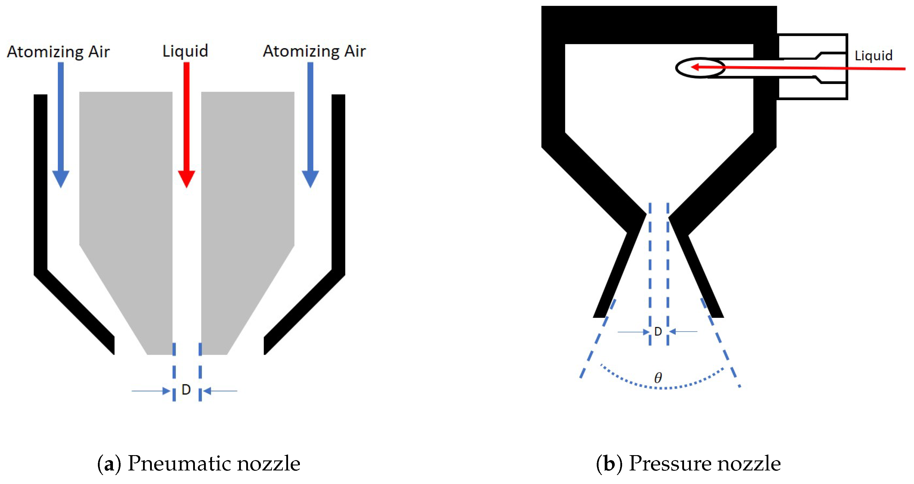
The model was evaluated considering two different spray nozzle configurations: (i) a pneumatic nozzle and (ii) a pressure nozzle. These two configurations were considered to evaluate the impact that the parameters influencing the droplet formation had on the properties of the particulate product. It was also intended to determine if a specific nozzle provided more robustness against any process variability. In a pneumatic nozzle, the gas at high velocity (around sonic) disperses the liquid into droplets. Although many different configurations are available within pneumatic nozzles, a nozzle with parallel flow was considered in this study (Figure 3a). In such nozzles, the droplet size is mainly determined by: (i) the nozzle dimensions, (ii) the liquid properties, (iii) the gas velocity, and (iv) the ratio between gas and liquid flows (ALR). An empirical estimate of the droplet size using these properties is given by Equation (40) [1].

$$\begin{array}{c}\hfill d_{32}=A{d}_n{\left[\frac{We}{{\left(1+\frac{1}{ALR}\right)}^2}\right]}^B\left(1+COh\right)\end{array}$$

(40)

Nozzle diameter and the air liquid ratio enter the above equation explicitly, while the air/liquid properties and gas velocity enters via the Ohnsorge ($Oh$) and Weber ($We$) numbers. The three empirical parameters $A,B,$ and C need to be determined through experimental data. In this study, the parameters determined in [1] were used. The dispersion of liquid due to the impact of a gas jet in a pneumatic nozzle occurred when the dynamic pressure of the gas exceeded the internal pressure of the droplets formed. In [37], it was established that the breakup of liquid started in the range $8<We<10$. The minimum required gas velocity in the nozzle can be computed from this condition, given the properties of the liquid.

In a pressure nozzle (Figure 3b), the droplets were formed by an abrupt pressure drop at the tip of the nozzle. At this point, the energy of the liquid upstream, in the form of pressure, was converted into velocity. Among the many pressure nozzle configurations available, the swirl atomizer type nozzle was considered in this study. The droplet size in this case was determined by the inner nozzle dimensions, the fluid properties, and the upstream pressure upstream. An empirical relation for this nozzle is given in Equation (41). This relation relates the droplet size to: (i) the nozzle diameter ($d_n$), (ii) pressure drop ($\Delta p$), (iii) fluid properties via the Reynolds number ($R{e}_p$), (iv) and the density ratio [37].

$$\begin{array}{c}\hfill \frac{d_{32}}{d_n}=2.3{\Psi }^{1/4}\Delta p^{*-1/4}R{e}_p^{-1/4}{\left(\frac{\rho }{{\rho }_a}\right)}^{1/4}\end{array}$$

(41)

The discharge coefficient ($\Psi$) of the swirl nozzle was calculated using the empirical correlation developed in [38]. The formation of small droplets depends on the formation of a thin sheet of liquid from the tip of the pressure nozzle. According to [37], this condition is achieved with low viscosity liquids for which $Oh<0.05$. Additionally, a minimum pressure is required to form this hyperbolic sheet in the swirl nozzles.

3. Results

Five main outputs were considered for the sensitivity analysis: (i) the final particle size, (ii) residual solvent content, (iii) particle density, (iv) maximum temperature, and (v) the distance in the chamber at which the equilibrium was reached (if it was reached). The first three outputs can be important CQAs, which need to be monitored. For temperature-sensitive products, the maximum temperature is an important factor to consider, as they might degrade at high temperatures. For the pressure nozzle, the upstream liquid pressure P was included to evaluate the flow energy requirement. The input parameters depending on the nozzle used and their ranges are given in

Table 1. Input and output variables considered for the sensitivity analysis with their ranges. Viscosity and upstream liquid pressure are considered only for the pressure nozzle, while ALR is considered only for the pneumatic nozzle.

	Variable	Symbol	Range of Variation	Units
Input variables	Flow of the liquid feed		$Q_l$	$5\times {10}^{-8}$–$2\times {10}^{-7}$	${\mathrm{m}}^3/\mathrm{s}$
	Flow of the drying gas		$M_{a,d}$	$8.5\times {10}^{-4}$–$8.5\times {10}^{-2}$	$\mathrm{kg}/\mathrm{s}$
	Initial Temp.of the gas		$T_{a,0}$	350–420	K
	Initial Temp. of the liquid		$T_{l,0}$	300–350	K
	Viscosity of the liquid		${\nu }_l$	$1\times {10}^{-3}$–$2\times {10}^{-2}$	Pa·s
	Air-to-liquid ratio	$ALR$	0.5–4	-
Output variables	Particle diameter		$d_p$	-	$\mathsf{\mu }\mathrm{m}$
	Residual solvent content		$W_p$	-	-
	Particle density		${\rho }_p$	-	$\mathrm{kg}/{\mathrm{m}}^3$
	Length for equilibrium		$Z_{eq}$	-	m
	Particle’s maximum temperature		$T_{p,max}$	-	K
	Upstream liquid pressure	P	-	bar

.

All the models were implemented in MATLAB 2017b (The MathWorks Inc., Natick, MA, USA). The system of differential equations was solved using a variable order variable step solver based on numerical difference formulas (ode15s), which is known to handle stiff systems well. The sensitivity indices were calculated using Saltelli’s approximation and PCE approximation. In the following sections, the two approximations are compared, and then an analysis on the spray drying process is provided.

3.1. Computation of Sensitivity Indices

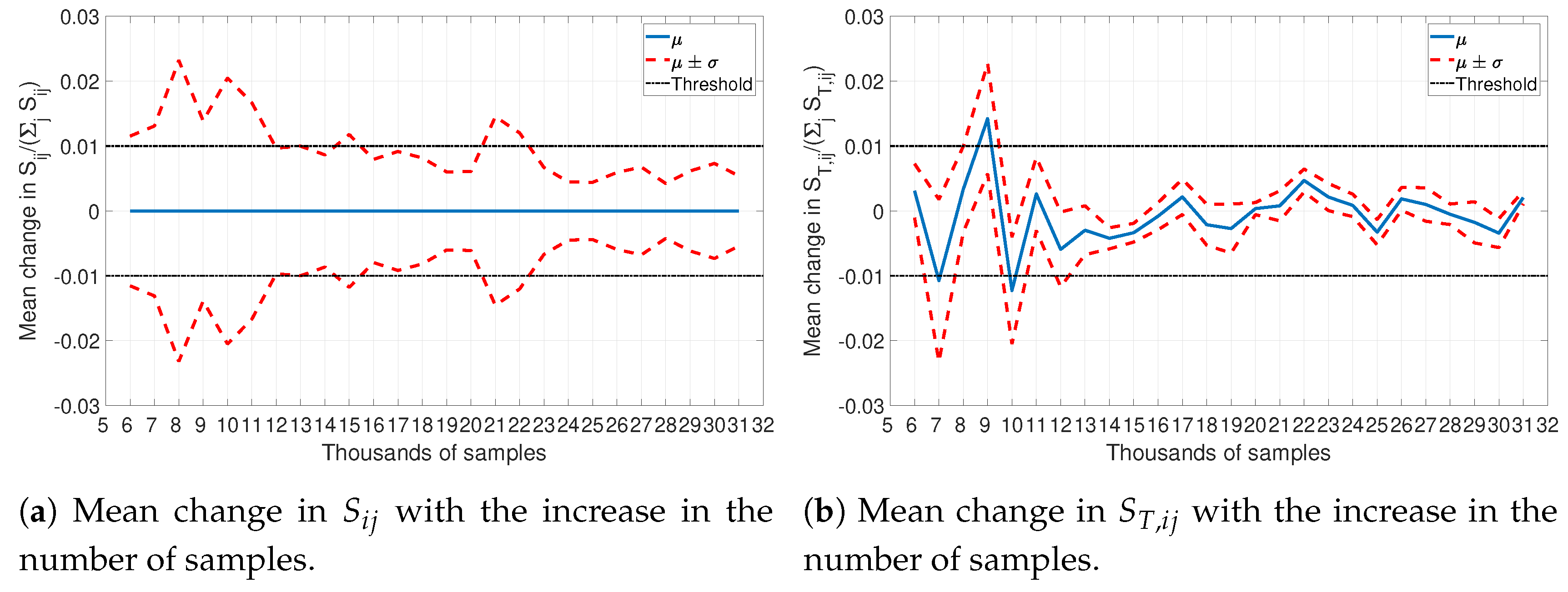
As analytical calculation of sensitivity indices is almost impossible for complex models, so an approximation based on pseudorandom sampling was used to get a good estimate. Traditionally, sampling-based methods assume that a large sample size (>10,000 samples) is enough to guarantee a valid solution. However, how many samples are enough is a difficult question to answer a priori. In this study, an approach with an iterative increase in the number of samples was used to determine the sample size. Starting from 5000 samples, the sample size was increased by 1000 samples at every iteration. A stopping criterion was defined based on the relative change of the normalized first order and total sensitivity indices. Figure 4 shows the evolution of the mean ($\mu$) and the standard deviation ($\sigma$) of the change in normalized sensitivity indices (first order, $\raisebox{1ex}{$S_{ij}$}\!\left/ \!\raisebox{-1ex}{${\sum }_j{S}_{ij}$}\right.$; and total $\raisebox{1ex}{$S_{T,ij}$}\!\left/ \!\raisebox{-1ex}{${\sum }_j{S}_{T,ij}$}\right.$) with the increasing number of samples. The number of samples was considered large enough when the the standard deviation in the relative change was less than $1\%$.

Based on Figure 4, a set of 23,000 samples was considered large enough for the approximation for a stable estimation of the sensitivity indices. Even though there were smaller sample sizes that met the criterion, it was only after 23,000 samples that the results seemed to stabilize below the defined threshold. With 23,000 samples and five input parameters, the calculation of sensitivity indices required around 161,000 function evaluations!As mentioned before, the current best practices suggest that the sensitivity indices calculated as above can be considered true values [23]. Thus, these will be used to compare the accuracy of sensitivity indices approximated by the PCE approach.

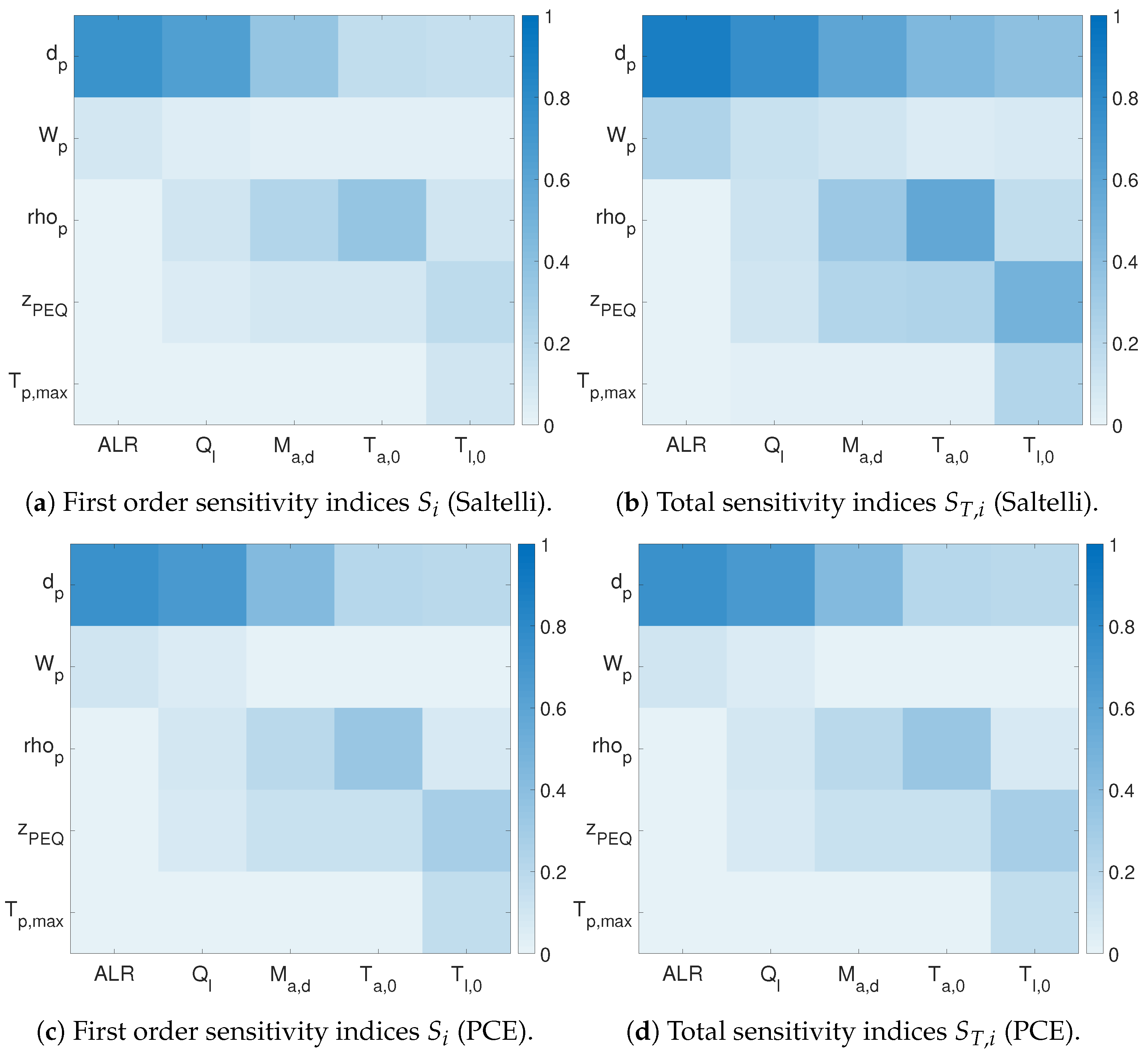
The PCE approach is a meta-modeling approach used to reduce the number of function evaluations. Figure 5 shows the results for the absolute sensitivity indices of the spray dryer operating with the pneumatic nozzle. The two heat maps at the top correspond to the sensitivity indices approximated using Saltelli’s method, and those at the bottom were approximated using PCE.

Table 2. Input ranking based on total sensitivity indices computed using Saltelli’s approximation (Sal) with 23,000 samples and third order PCE with 200 samples.

Rank	dp		Wp		${\rho }_p$		Zeq		$T_{p_{max}}$
	Sal	PCE	Sal	PCE	Sal	PCE	Sal	PCE	Sal	PCE
$ALR$	1	1	1	1	1	1	2	2	2	2
$Q_l$	2	2	2	2	4	4	4	4	4	4
$M_{a,d}$	-	-	2	2	2	2	1	1	3	3
$T_{a,0}$	-	-	3	3	3	3	3	3	1	1
$T_{l,0}$	-	-	-	-	-	-	-	-	4	3

presents the input ranking based on the total sensitivity indices.

The rank was assigned assuming that a difference smaller than $5\%$ between the sensitivity indices was insignificant. Consequently, any sensitivity index below 0.05 was considered equal to zero and the output assumed to be independent of the input. Similarly, the same rank was given to multiple inputs whose sensitivity indices did not differ significantly.

The input ranking obtained by both the Saltelli and PCE approach was the same, except for the output $T_{p,max}$. In this case, although the first order sensitivity indices were comparable, total sensitivity indices showed significant variation from the ones calculated by Saltelli’s method. A plausible reason for this could be that $T_{p,max}$ was extremely nonlinear in inputs, and the correct estimation would require a higher order polynomial. This is evident from

Table 3. Change in total sensitivity indices ($S_{T,i}$) for $T_{p,max}$ with increasing polynomial order (p) in the PCE approach.

Parameter	PCE $(p=3)$	PCE $(p=4)$	PCE $(p=5)$	PCE $(p=6)$	PCE $(p=7)$	Saltelli
$ALR$	0.3826	0.4481	0.4444	0.5030	0.5031	0.4920
$Q_l$	0.0706	0.1652	0.1789	0.2975	0.2352	0.2350
$M_{a,d}$	0.1596	0.2315	0.3127	0.3825	0.3498	0.3582
$T_{a,0}$	0.4883	0.4626	0.4463	0.5011	0.4728	0.5352
$T_{l,0}$	0.2341	0.2514	0.2939	0.1907	0.2964	0.2289
# of Samples	200	400	600	1000	2000	23,000
# of Function Evaluations	200	400	600	1000	2000	161,000

. With increasing order, nonlinearity was captured with much more ease. However, the number of samples required to evaluate the sensitivity indices also increased with the order of the PCE. The benefits on computational time provided by the PCE approach outweighed the slight decrease in accuracy. Even if a high order PCE was used, the number of function evaluation was at least an order of magnitude less than the number of function evaluations for Saltelli’s approach.

3.2. Global Sensitivity Analysis of Spray Dryer with a Pneumatic Nozzle

Based on the previous discussion and to avoid excessive computational costs, the PCE approach was used for the sensitivity analysis of the two spray dryers. A fourth order PCE was used to determine the sensitivity indices, and 600 samples were used to compute the coefficients of the expansion.

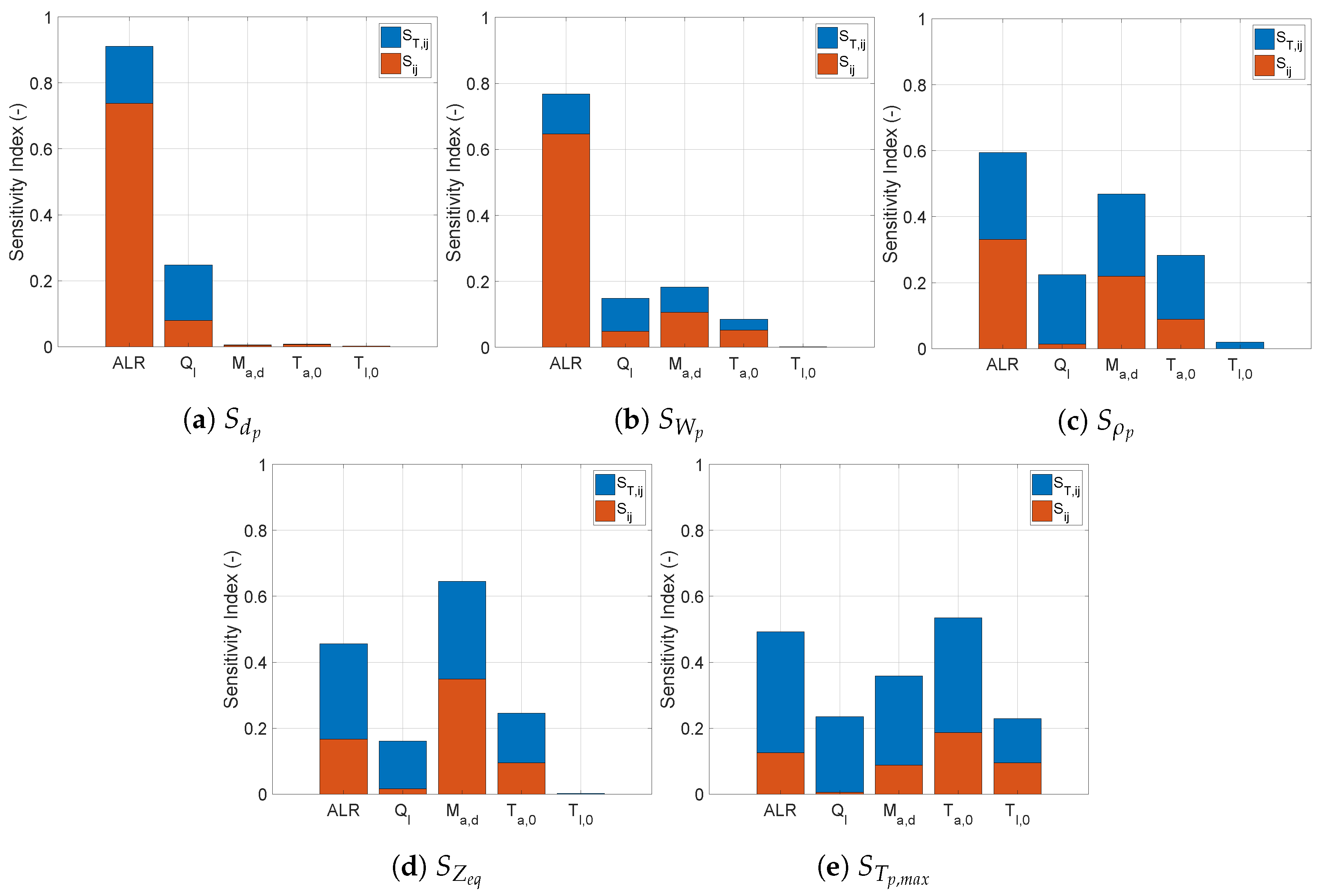
Figure 6 depicts the sensitivity indices for a spray dryer operating with the pneumatic nozzle.

Based on the response to the inputs depicted in Figure 6, the output variables could be divided into two groups. The first group consisted of the variables whose responses were mostly determined by the individual change of a single input. The other group contained outputs whose response involved significant high order input interactions. In the first group, the particle diameter and the residual humidity were characterized by a strong first order effect from the ALR along with a minor influence from the other inputs. For the particle size, only the liquid flow rate had a significant effect apart from the ALR. For the residual solvent content, the flow rate and temperature of the drying air played a minor role. This means that in a spray dryer equipped with a pneumatic nozzle, the final particle size and residual humidity were conditioned by the droplet formation, which was determined by the amount of atomization gas used with the liquid flow rate.

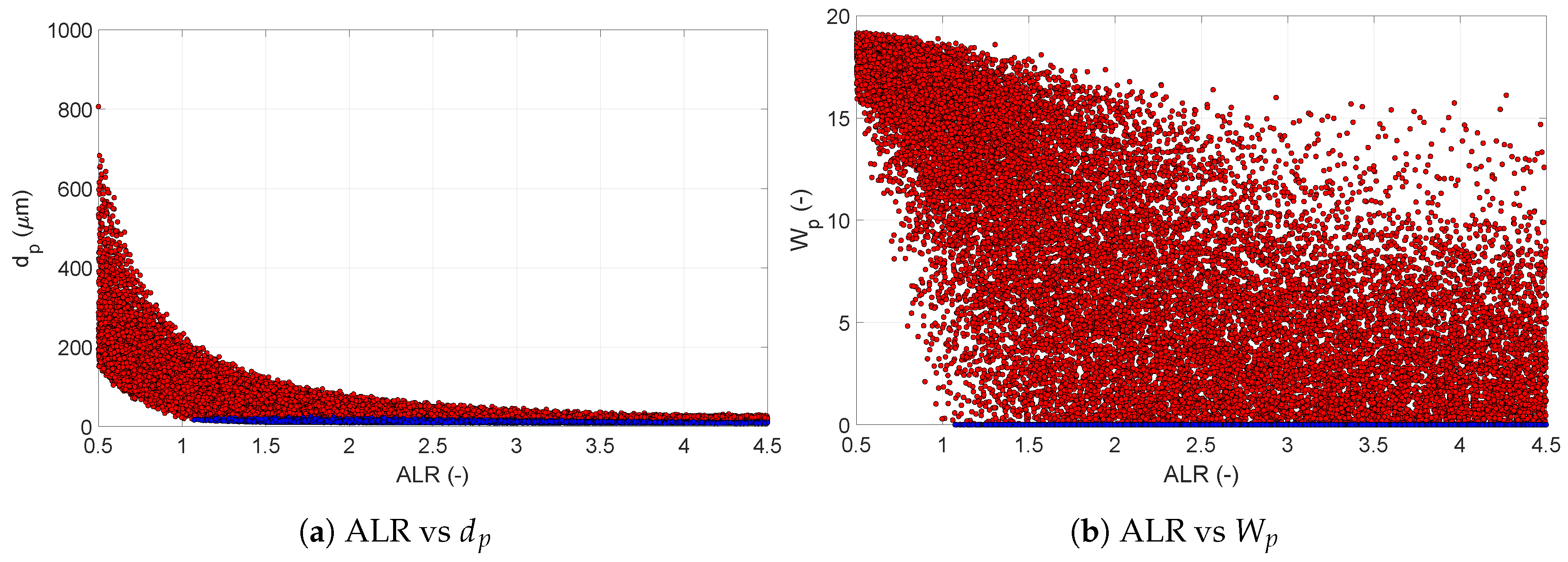
In Figure 7, the scatter plots illustrate the solutions for $d_p$ and $W_p$, from which samples were taken to perform the sensitivity calculations. The blue dots correspond to a product that has reached its drying equilibrium, while red dots correspond to non-equilibrium. It can be noticed that most of the variation occurred at non-equilibrium conditions. It can also be seen that the ALR determined whether equilibrium was reached, and equilibrium was reached only at high ALR. The low spread in the particle size data showed that the particle size was mostly dominated by the ALR. With the increase in the ALR, the spread of the final particle size reduced, and the possible solutions tended to concentrate close to the equilibrium solution. This is the result of the small droplet size obtained from the pneumatic nozzle at high ALR. Since the droplet size was already very close to the equilibrium size of the particle, other conditions in the process did not have a major impact, and the spread of the possible end particle size was very narrow. Differently, in the case of the residual solvent $W_p$, its large spread of solutions indicated that other inputs remained influential at any value of ALR. For high ALR, the final humidity of the particle at a non-equilibrium condition would depend also on the number of droplets in the chamber; the larger the number of droplets, the more solvent needed to evaporate to reduce their humidity. Thus, for the pneumatic nozzle, the particle size could be tuned solely by the ALR, whereas an accurate control over the residual solvent content required tuning the liquid feed rate as well.

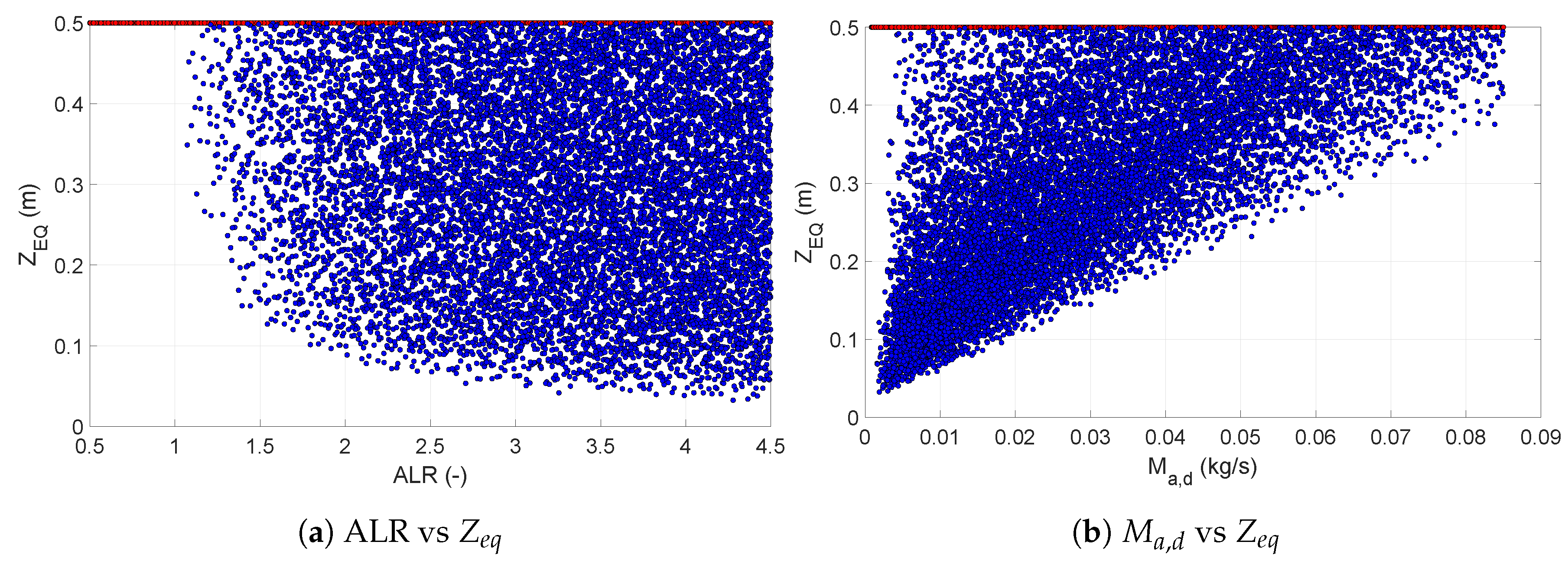
For the second group of outputs (${\rho }_p$, $Z_{eq}$, and $T_{p,max}$), the ALR was not the sole significant input. The contributions of other inputs varied with every output, but a similarity could be observed between the responses of ${\rho }_p$ and $Z_{eq}$. As could be expected, the input temperature played a greater role in the determining the maximum particle temperature. The liquid feed temperature was relevant only for $T_{p,max}$. Figure 8 presents the scatter plots of the length required to reach equilibrium with respect to $ALR$ and $M_{a,d}$. The scatter plots confirmed that ALR had a significant influence on the point at which the equilibrium was reached. For ALR below one, all solutions were in the non-equilibrium region. Once this threshold value of ALR was crossed, the scatter suggested that the point at which the equilibrium was reached was determined by more factors than just the ALR. The scatter plot for the relation between $Z_{eq}$ and $M_{a,d}$ showed that an increase in the amount of drying air tended to move the equilibrium point towards the bottom of the dryer.

3.3. Global Sensitivity Analysis of the Spray Dryer with a Pressure Nozzle

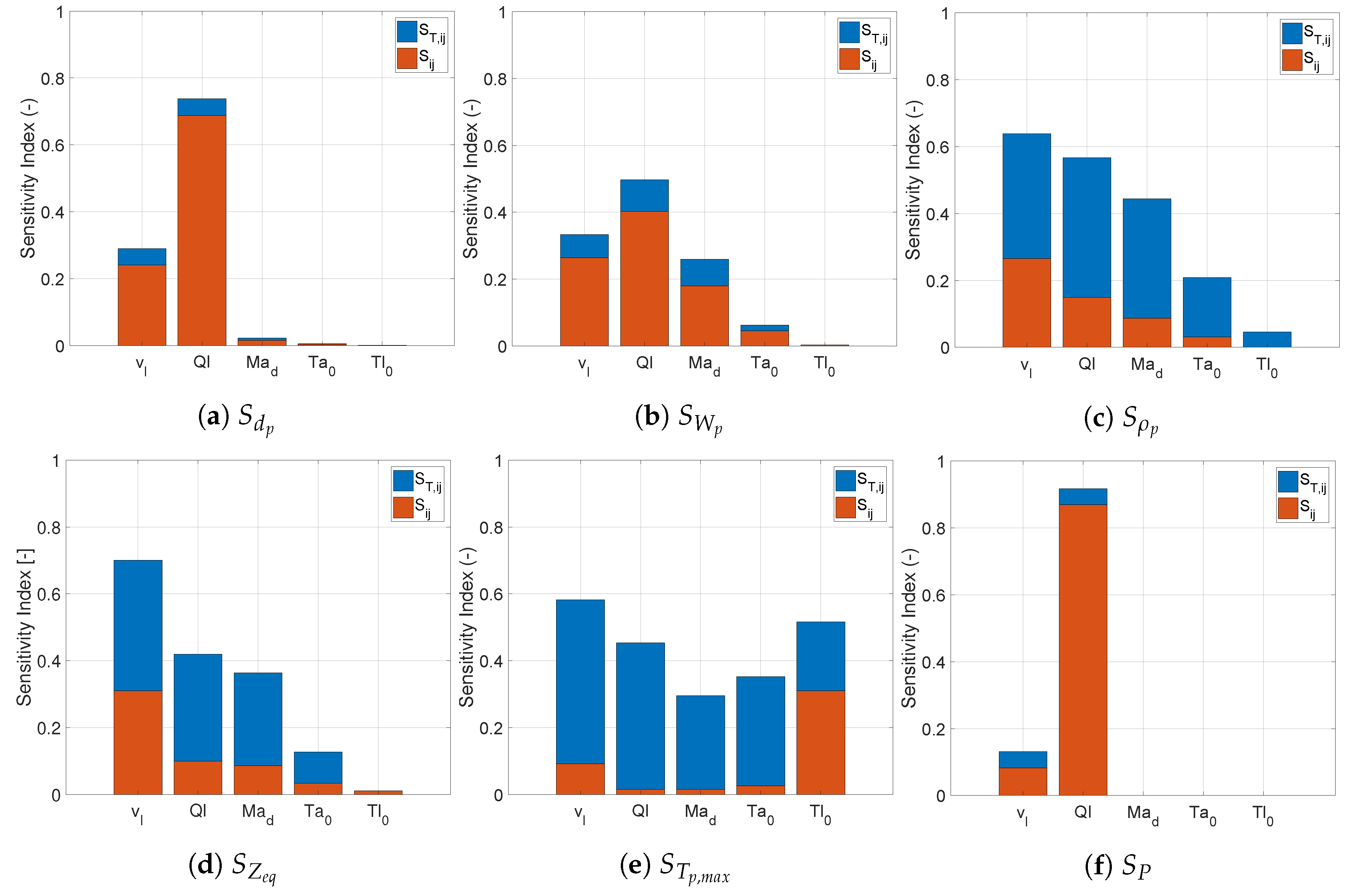
Figure 9 depicts the sensitivity indices for the spray dryer operating with a pressure nozzle.

Analogously to the pneumatic nozzle, the outputs could be divided into two groups. The first group consisted of the particle diameter and the upstream liquid pressure, which were dominated by first order effects corresponding to the droplet formation. For liquid feed pressure, this was expected, as the pressure required for the liquid to go through the nozzle was independent of the drying. Contrary to the pneumatic nozzle, the residual solvent content was not part of this group. Since there was no additional process parameter affecting the droplet formation, the feed flow rate $Q_l$ became the most influential variable for the end particle size.

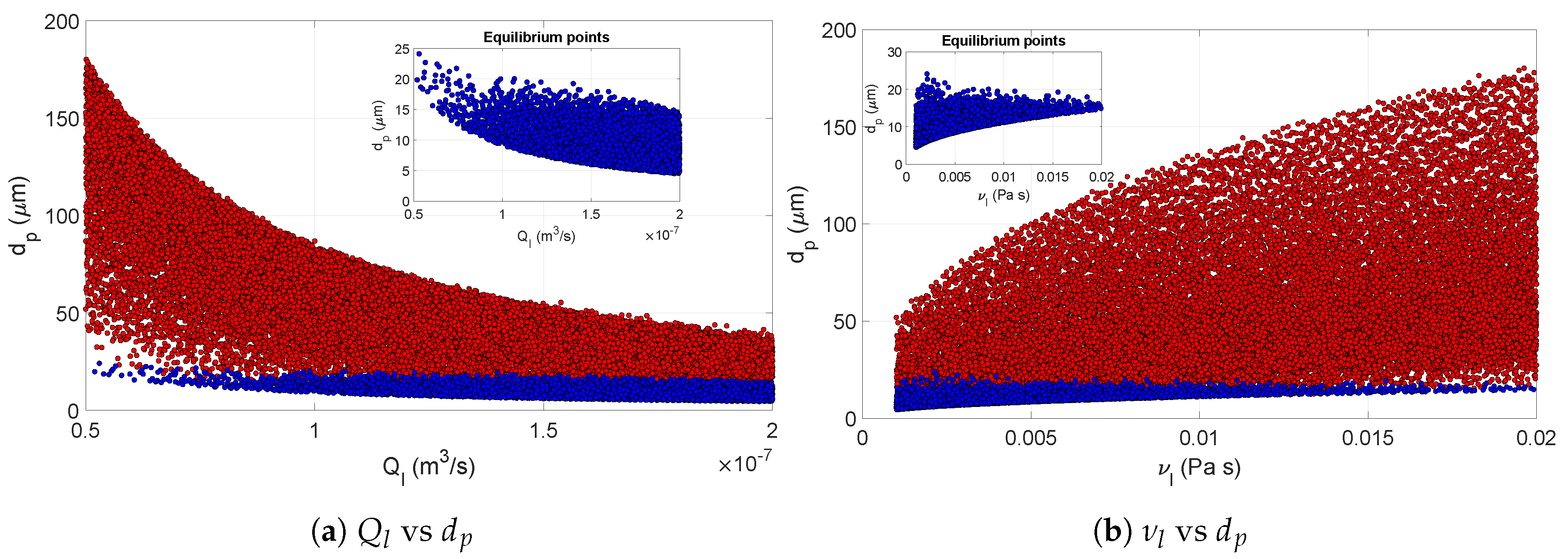
Along with $Q_l$, the viscosity of the liquid also had a significant effect on the particle diameter. In practice, the variation in the feed flow might be intentional or induced by uncontrolled variability in the nozzle characteristics when the spray dryer is operated at a fixed upstream pressure. The variability of the viscosity might be uncontrolled due to the properties of the material added to the feed mixture. Figure 10 depicts the scatter of $d_p$ with respect to $Q_l$ and ${\nu }_l$. The dependence of the particle size on these two variables is clearly visible from these figures. Additionally, these relations were also maintained in equilibrium conditions. However, at equilibrium, the variation was reduced. The narrow spread of the $d_p$ scatter for $Q_l$ explained the significance of $Q_l$.

The residual solvent content showed a higher level of interaction between the droplet formation and the drying process. The contributions were distributed along the evaluated process conditions. Along with the feed flow rate and viscosity, the flow rate of drying air and its initial temperature also had a significant impact on the residual solvent content.

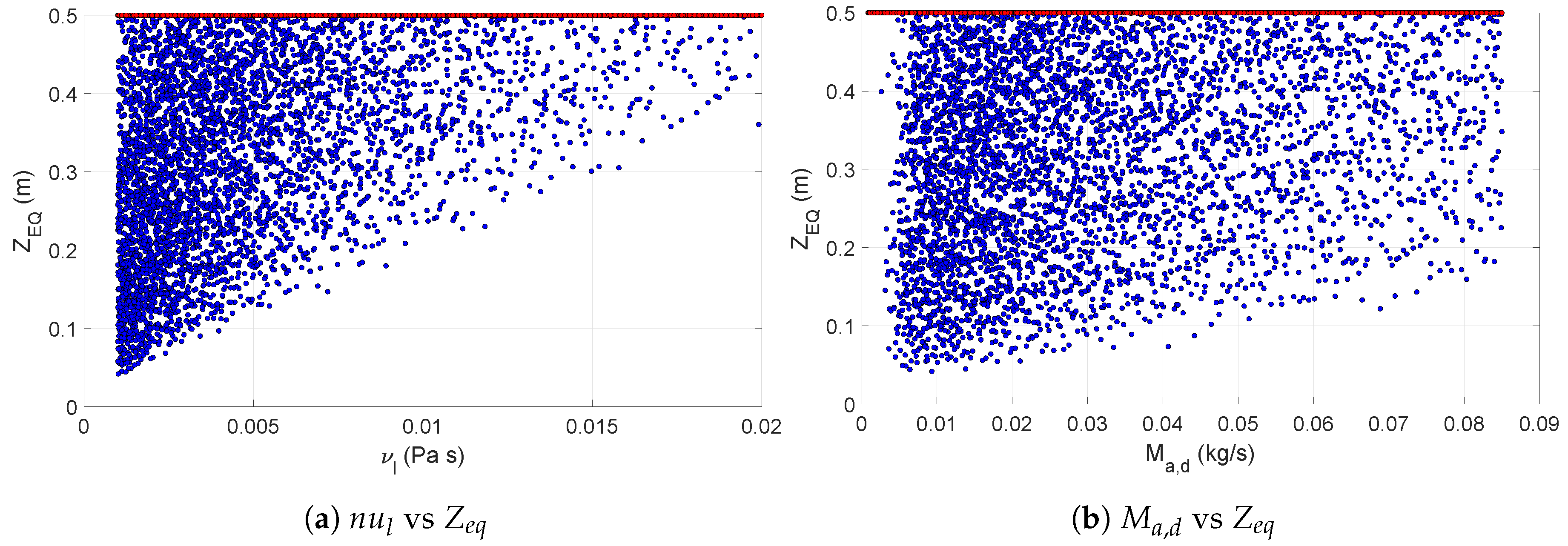
The second group consisted of particle density, the distance at which equilibrium was reached, and the maximum temperature reached. As was the case with the pneumatic nozzle, the sensitivity profile of ${\rho }_p$ and $Z_{eq}$ for the pressure nozzle was also similar. These two outputs showed high sensitivity to the viscosity, the feed flow rate, and the flow rate of drying gas. Figure 11 shows the scatter of $Z_{eq}$ with respect to ${\nu }_l$ and $M_{a,d}$. The former can easily be identified as the most influential parameter. In Figure 11, the scatter cloud was made primarily of blue dots, i.e., results achieving equilibrium at different lengths inside the drying chamber, and all other results at a non-equilibrium condition had a value $Z_{eq}=0.5\mathrm{m}$. This shows that for product leaving the dryer at equilibrium, the viscosity had a major impact on the particle size, and in turn also on the length required to reach the equilibrium. Figure 11 illustrates how the same drying parameter might affect in a different way an output variable due to the difference in the interactions with the parameters from the two different nozzles. The direct comparison of this plot with its equivalent in Figure 8 shows that $M_{a,d}$ had a much more significant individual impact on $Z_{eq}$ for the pneumatic nozzle. In case of the pressure nozzle, the velocity of the droplets in the dryer chamber was influenced both by the pressure drop $\left(P\right)$ in the nozzle and the $M_{a,d}$ determining the velocity of the gas in the chamber, leading to a much more entropic scatter.

4. Conclusions

Based on the discussion above, it can be concluded that PCE was an attractive approach to reduce the computational burden required for a global sensitivity analysis. The quantitative values of the sensitivity indices computed using PCE approach, although different, were still comparable to Saltelli’s approximation. The input ranking obtained, which was arguably more important than the quantitative values themselves, was the same if a proper PCE order was used. It has to be noted that if the process were highly nonlinear, a low order PCE could lead to erroneous results. However, there is no a priori way of determining the nonlinearity associated with any output. In such situations, an iterative approach with increasing the order of PCE is recommended. Even with such an iterative approach, the number of function evaluations required for the PCE approach were orders of magnitude fewer than the quasi Monte Carlo approach. For the case study considered above, use of a fourth order PCE instead of a stable quasi Monte Carlo approach led to around a 99.6% reduction in computational cost. Even if a seventh order PCE was used, the computational savings were around 96%.

The GSA of the spray drying model allowed the system to be characterized based on the dominant relationships between the CQAs and the CPPs. This analysis provides a detailed view on how the phenomena occurring during atomization and drying interact and determine the output response. Based on this study, it was possible to discriminate the behavior of the spray dryer depending on the type of nozzle.

The sensitivity patterns demonstrated that independent of the nozzle used, mean particle size was affected predominantly by the atomization phenomena, while others’ outputs were affected by an interaction between the atomization and drying parameters. The type of nozzle to be used will always depend on the application. Given the presence of the ALR, the pneumatic nozzle had more flexibility for the control of the final particle size. However, this also meant that a tight ALR control was required as a small variance on this parameter would have a large impact on the particle size. For the pressure nozzle, a strong dependency was established along all outputs on the feed flow rate, which additionally will determine the throughput of the unit. This dependency was strengthened by the fact that both the initial droplet size and velocity were extremely affected by changes in the liquid flow rate. This diminished the effect of the drying parameters. This was specifically clear for particle density and the distance to reach equilibrium. The direct effect of the drying flow rate for these two outputs was found to be less important in the case of the pressure nozzle compared to the pneumatic nozzle.

Future work will be focused on applying other computational intelligence methods, e.g., fuzzy logic and genetic programming, to compare their performance for GSA, but also for knowledge discovery purposes.

References

- Cotabarren, I.M.; Bertín, D.; Razuc, M.; Rairez-Rigo, M.V.; Pina, J. Modelling of the spray drying process for particle design. Chem. Eng. Res. Des. 2018, 132, 1091–1104. [Google Scholar] [CrossRef]
- Schuck, P.; Jeantet, R.; Bhandari, B.; Chen, X.D.; Perrone, Í.T.; de Carvalho, A.F.; Fenelon, M.; Kelly, P. Recent advances in spray drying relevant to the dairy industry: A comprehensive critical review. Dry. Technol. 2016, 34, 1773–1790. [Google Scholar] [CrossRef]
- Shishir, M.R.I.; Chen, W. Trends of spray drying: A critical review on drying of fruit and vegetable juices. Trends Food Sci. Technol. 2017, 65, 49–67. [Google Scholar] [CrossRef]
- Poozesh, S.; Bilgili, E. Scale-up of pharmaceutical spray drying using scale-up rules: A review. Int. J. Pharm. 2019, 562, 271–292. [Google Scholar] [CrossRef] [PubMed]
- Sosnik, A.; Seremeta, K.P. Advantages and challenges of the spray-drying technology for the production of pure drug particles and drug-loaded polymeric carriers. Adv. Colloid Interface Sci. 2015, 223, 40–54. [Google Scholar] [CrossRef] [PubMed]
- Fatnassi, M.; Tourné-Péteilh, C.; Peralta, P.; Cacciaguerra, T.; Dieudonné, P.; Devoisselle, J.M.; Alonso, B. Encapsulation of complementary model drugs in spray-dried nanostructured materials. J. Sol-Gel Sci. Technol. 2013, 68, 307–316. [Google Scholar] [CrossRef]
- Cheow, W.S.; Li, S.; Hadinoto, K. Spray drying formulation of hollow spherical aggregates of silica nanoparticles by experimental design. Chem. Eng. Res. Des. 2010, 88, 673–685. [Google Scholar] [CrossRef]
- Gharsallaoui, A.; Roudaut, G.; Chambin, O.; Voilley, A.; Saurel, R. Applications of spray-drying in microencapsulation of food ingredients: An overview. Food Res. Int. 2007, 40, 1107–1121. [Google Scholar] [CrossRef]
- Vincente, J.; Pinto, J.; Menezes, J.; Gaspar, F. Fundamental analysis of particle formation in spray drying. Powder Technol. 2013, 247, 1–7. [Google Scholar] [CrossRef]
- Nandiyanto, A.B.D.; Okuyama, K. Progress in developing spray-drying methods for the production of controlled morphology particles: From the nanometer to submicrometer size ranges. Adv. Powder Technol. 2011, 22, 1–19. [Google Scholar] [CrossRef]
- Debevec, V.; Srčič, S.; Horvat, M. Scientific, statistical, practical, and regulatory considerations in design space development. Drug Dev. Ind. Pharm. 2018, 44, 349–364. [Google Scholar] [CrossRef] [PubMed]
- Petersen, L.N.; Poulsen, N.K.; Niemann, H.H.; Utzen, C.; Jørgensen, J.B. An experimentally validated simulation model for a four-stage spray dryer. J. Process Control 2017, 57, 50–65. [Google Scholar] [CrossRef] [Green Version]
- Ferrari, A.; Gutiérrez, S.; Sin, G. Modeling a production scale milk drying process: Parameter estimation, uncertainty and sensitivity analysis. Chem. Eng. Sci. 2016, 152, 301–310. [Google Scholar] [CrossRef]
- Zhang, X.; Pei, Y.; Xie, D.; Chen, H. Modeling Spray Drying of Redispersible Polyacrylate Powder. Dry. Technol. 2014, 32, 222–235. [Google Scholar] [CrossRef]
- Mezhericher, M.; Levy, A.; Borde, I. Multi-Scale Multiphase Modeling of Transport Phenomena in Spray-Drying Processes. Dry. Technol. 2015, 33, 2–23. [Google Scholar] [CrossRef]
- Juaber, H.; Afshar, S.; Xiao, J.; Chen, X.D.; Selomulya, C.; Woo, M.W. On the importance of droplet shrinkage in CFD-modeling of spray drying. Dry. Technol. 2018, 36, 1785–1801. [Google Scholar] [CrossRef]
- Baldinger, A.; Clerdent, L.; Rantanen, J.; Yang, M.; Grohganz, H. Quality by design approach in the optimization of the spray-drying process. Pharm. Dev. Technol. 2012, 17, 389–397. [Google Scholar] [CrossRef]
- Lebrun, P.; Krier, F.; Mantanus, J.; Grohganz, H.; Yang, M.; Rozet, E.; Boulanger, B.; Evrard, B.; Rantanen, J.; Hubert, P. Design space approach in the optimization of the spray-drying process. Eur. J. Pharm. Biopharm. 2012, 80, 226–234. [Google Scholar] [CrossRef]
- Razuc, M.; Piña, J.; Ramírez-Rigo, M.V. Optimization of Ciprofloxacin Hydrochloride Spray-Dried Microparticles for Pulmonary Delivery Using Design of Experiments. AAPS PharmSciTech 2018, 19, 3085–3096. [Google Scholar] [CrossRef]
- Ingvarsson, P.T.; Yang, M.; Mulvad, H.; Nielsen, H.M.; Rantanen, J.; Foged, C. Engineering of an inhalable dda/tdb liposomal adjuvant: A quality-by-design approach towards optimization of the spray drying process. Pharm. Res. 2013, 30, 2772–2784. [Google Scholar] [CrossRef]
- Sobol, I. Global sensitivity indices for nonlunear mathematical modesl and their Monte Carlo estimates. Math. Comput. Simul. 2001, 55, 271–280. [Google Scholar] [CrossRef]
- Saltelli, A.; Ratto, M.; Andres, T.; Campolongo, F.; Cariboni, J.; Gatelli, D.; Saisana, M.; Tarantola, S. Global Sensitivity Analysis: The Primer; John Wiley & Sons Ltd.: Chichester, UK, 2008. [Google Scholar]
- Saltelli, A.; Annoni, P.; Azzini, I.; Campolongo, F.; Ratto, M.; Tarantola, S. Variance based sensitivity analysis of model output. Design and estimator for the total sensitivity index. Comput. Phys. Commun. 2010, 181, 259–270. [Google Scholar] [CrossRef]
- Todri, E.; Amenaghawon, A.; Jimenez del Val, I.; Leak, D.; Kontoravdi, C.; Kucherenko, S.; Shah, N. Global sensitivity analysis and meta-modeling of an ethanol production process. Chem. Eng. Sci. 2014, 114, 114–127. [Google Scholar] [CrossRef]
- Crestaux, T.; Le Maître, O.; Martinez, J.M. Polynomial chaos expansion for sensitivity analysis. Reliab. Eng. Syst. Saf. 2009, 94, 1161–1172. [Google Scholar] [CrossRef]
- Blatman, G.; Sudret, B. Efficient computation of global sensitivity indices using sparse polynomial chaos expansions. Reliab. Eng. Syst. Saf. 2010, 95, 1216–1229. [Google Scholar] [CrossRef]
- Sudret, B. Global sensitivity analysis using polynomial chaos expansions. Reliab. Eng. Syst. Saf. 2008, 93, 964–979. [Google Scholar] [CrossRef]
- Negiz, A.; Lagergren, E.S.; Cinar, A. Mathematical models of cocurrent spray drying. Ind. Eng. Chem. Res. 1995, 34, 3289–3302. [Google Scholar] [CrossRef]
- Ranz, W.; Marshall, W. Evaporation from drops. Parts I and II. Chem. Eng. Prog. 1952, 48, 141–146, 173–180. [Google Scholar]
- Homma, T.; Saltelli, A. Importance measures in global sensitivity analysis of nonlinear models. Reliab. Eng. Syst. Saf. 1996, 52, 1–17. [Google Scholar] [CrossRef]
- Xiu, D.; Karniadakis, G. The Wiener–Askey polynomial chaos for stochastic differential equations. SIAM J. Sci. Comput. 2002, 24, 619–644. [Google Scholar] [CrossRef]
- Oladyshkin, S.; Nowak, W. Data-driven uncertainty quantification using the arbitrary polynomial chaos expansion. Reliab. Eng. Syst. Saf. 2012, 106, 179–190. [Google Scholar] [CrossRef]
- Yang, S.; Xiong, F.; Wang, F. Polynomial Chaos Expansion for Probabilistic Uncertainty Propagation. In Uncertainty Quantification and Model Calibration; Hessling, J.P., Ed.; IntechOpen: Rijeka, Croatia, 2017; Chapter 2. [Google Scholar] [Green Version]
- Bhonsale, S.; Nimmegeers, P.; Telen, D.; Paulson, J.A.; Mesbah, A.; Van Impe, J. On the implementation of generalized polynomial chaos in dynamic optimization under stochastic uncertainty: A user perspective. In Computer Aided Chemical Engineering; Kiss, A.A., Zondervan, E., Lakerveld, R., Özkan, L., Eds.; Elsvier: Rijeka, Croatia, 2017; Chapter 1. [Google Scholar]
- Nimmegeers, P.; Telen, D.; Logist, F.; Van Impe, J. Dynamic optimization of biological networks under parametric uncertainty. BMC Syst. Biol. 2016, 10, 86. [Google Scholar] [CrossRef] [PubMed]
- Bhonsale, S.; Telen, D.; Stokbroekx, B.; Van Impe, J. An Analysis of Uncertainty Propagation Methods Applied to Breakage Population Balance. Processes 2018, 6, 255. [Google Scholar] [CrossRef]
- Walzel, P. Spraying and Atomization of liquids. In Ullmann’s Encyclopedia of Industrial Chemestry; Wiley-VCH Verlag GmbH: Weinheim, Germany, 2012; pp. 79–98. [Google Scholar]
- Wimmer, E.; Brenn, G. Viscous effects on flows through pressure-swirl atomizers. In Proceedings of the 12th Triennial International Conference on Liquid Atomization and Spray Systems (ICLASS 2012), Heidelberg, Germany, 2–6 September 2012. [Google Scholar]
Figure 1.
Schematic of a spray dryer.
Figure 2.
Example of the spray drying output evolution along the length of the drying chamber at nominal conditions.
Figure 3.
Schematics of the two different nozzles of diameter D.
Figure 4.
Stability of the sensitivity indices calculated by Saltelli’s approximation. The mean change is defined as , where is the number of samples considered.
Figure 5.
Qualitative comparison of sensitivity heat maps for a spray dryer with the pneumatic nozzle computed using Saltelli’s approximation with 23,000 samples and third order PCE with 200 samples. The x-axis shows the operating parameters, and the y-axis shows the output parameters considered.
Figure 6.
Sensitivity indices () for the spray dryer operating with a pneumatic nozzle calculated using fourth order PCE with 600 samples.
Figure 7.
Scatter plots of final particle size (a) and residual moisture content with respect to ALR (b). The red dots indicate the values at non-equilibrium conditions, while blue dots represent the values at equilibrium. The figures clearly indicate the significant effect ALR has on particle size, along with its effect on residual solvent content. This effect is, however, limited only to the non-equilibrium zone.
Figure 8.
Scatter plots of equilibrium length with respect to ALR (a) and the mass flow rate of the drying air (b). The red dots indicate the values at non-equilibrium conditions, while blue dots represent the values at equilibrium.
Figure 9.
Sensitivity indices () for the spray dryer operating with a pressure nozzle calculated using fourth order PCE with 600 samples.
Figure 10.
Scatter plots of final particle size with respect to feed flow rate (a) and feed viscosity (b). The red dots indicate the values at non-equilibrium conditions, while blue dots represent the values at equilibrium. The equilibrium points are also shown explicitly in the insets. Unlike the pneumatic nozzle, the pressure nozzle conditions also influence the equilibrium values.
Figure 11.
Scatter plots of equilibrium length with respect to the feed viscosity (a) and mass flow rate of the drying air (b). The red dots indicate the values at non-equilibrium conditions, while blue dots represent the values at equilibrium.