GC-MS Fingerprints Profiling Using Machine Learning Models for Food Flavor Prediction


1
Department of Chemical Engineering, Tsinghua University, Beijing 100084, China
2
Beijing Key Laboratory of Industrial Big Data System and Application, Beijing 100084, China
3
COFCO Nutrition Health Research Institute, Beijing 102209, China
4
School of Food Science and Technology, Dalian Polytechnic University, Dalian 116034, China
*
Authors to whom correspondence should be addressed.
Processes 2020, 8(1), 23; https://0-doi-org.brum.beds.ac.uk/10.3390/pr8010023
Submission received: 23 November 2019
/
Revised: 15 December 2019
/
Accepted: 19 December 2019
/
Published: 23 December 2019
(This article belongs to the Special Issue Process Optimization and Control)
Abstract
:Food flavor quality evaluation is attracting continuous attention, but a suitable evaluation system is severely lacking. Gas chromatography-mass spectrometry/olfactometry (GC-MS/O) is widely used to solve the food flavor evaluation problem, but the olfactometry evaluation is unfeasible to be carried out in large batches and is unreliable due to potential issue of an operator or systematic laboratory effect. Thus, a novel fingerprint modeling and profiling process was proposed based on several machine learning models including convolutional neural network (CNN). The fingerprint template was created by the data analysis of existing GC-MS spectrum dataset. Then the fingerprint image generation program was applied for structuring the complex instrumental data. Food olfactometry result was obtained by a machine learning method based on CNN using fingerprint image as the input. The case study on peanut oil samples demonstrated the model accuracy of around 93%. By structure optimization and further dataset expansion, the whole process has the potential to be utilized by sensory laboratories for aroma analysis instead of humans.
1. Introduction
With the improvement of living standards, food flavor has been paid more and more attention. However, a mature food flavor quality evaluation standard has not been proposed until now. The research of odor compounds, aroma attributes, and aroma contribution in food products is essential for the comprehension of scent formation mechanism, the improvement of product quality, and the development of evaluation systems [1].
To analyze the aroma and odor compounds in food product, instrumental techniques are primary recommended methods instead of the fuzzy evaluation by traditional human-based qualitative analysis [2]. Among these instrumental analysis methods, gas chromatography-mass spectrometry/olfactometry (GC-MS/O) is an advanced sensory evaluation process which combines the advantages of instruments and humans and it provides a comprehensive analysis result [3]. In addition to the traditional GC-MS analysis, a split vent is installed in the end of the chromatography column, and some airflow of different odors will be transmitted to a human’s nose with moist air through an olfactory detector outlet [4]. After collecting chromatograms, mass spectra, and human olfactory results of a specific sample, a complete set of GC-MS/O data can be obtained and post-processed.
Recently, there were several researchers focusing on the correlation between the aroma of different types of food or daily chemicals and GC-MS/O data. M. Thomsen [5] investigated the semi-hard cheese aroma by GC-O analysis, applying principal components analysis (PCA) to divide the cheese samples by significant sensory odor attributes and partial least squares regression (PLSR) to make a correlation between sensory attributes and odor-active compounds. Pang, X. [6] introduced odor activity values (OAVs) and detection frequency analysis (DFA) methods to complete the identification of aroma-active compounds in Jiashi Muskmelon. These communications demonstrated that GC-MS/O analysis is a practical approach to evaluate the sensory attributes of typical food. However, olfactometry measurement is highly expensive in labor costs and might have adverse effects on human health due to the harmful chemicals in samples [7]. Potential issues of an operator or systematic laboratory effect may also exist during the GC-MS/O result analysis [2], especially the process of compounds filtration of mass spectrometry. Additionally, the regression methods based on a multiple linear regression model are not able to make sufficient utilization of dataset, and the stability and accuracy of the result cannot be guaranteed.
To make a relevant and valid prediction of the food sensory attributes, machine learning approaches are worth trying. Convolutional neural network (CNN) has been a hot discussion topic in recent years, such as GoogLeNet [8] proposed by Google Inc., Resnet [9] proposed by Microsoft Corporation. These CNN models are mature technologies for regression or classification, which extract features from images and map the features to a new space [10]. The unique patterns of GC-MS data in a specific sample can be obtained by fingerprint image generation process and recognized by a well-trained CNN model to forecast the odor of the sample and its retention time. A specific case study on peanut oil chemometrics analysis and sensory evaluation is performed. The peanut oil market has a huge consumption potential in China. Besides, the unique aroma of peanut oil is the main reason of the great popularity among Chinese people, and the odor compounds in peanut oil are receiving increasing attention from industry and research institutes [11].
In this paper, the whole process of converting GC-MS spectrum into olfactometry results is introduced, including instrumental and sensory analysis, odor compounds’ identification, GC-MS data structuring process by fingerprint image generation, and machine learning forecasting. Peanut oil samples are applied to demonstrate the characteristic of the model. In addition, the CNN model is optimized by structure design and the whole process can be applied in a laboratory.
2. Experimental Section
2.1. Material and Sample Preparation
Different brands of peanut oil were obtained from supermarkets in China with similar production dates. Headspace-solid phase microextraction (HS-SPME) technology [12] was applied to accomplish the pretreatment procedure of GC-MS/O analysis. Peanut oil sample (3 g) in a 30 mL vial was extracted by a 50/30 µm, 2 cm divinylbenzene (DVB)/carboxen (CAR)/polydimethylsiloxane (PDMS) fiber (Supelco, Bellafonte, KY, USA). The samples were firstly kept at 70 °C for 20 min at a stirring rate of 550 rpm to achieve gas–liquid equilibrium. Then the fiber stretched into the vial and complete adsorption and absorption at 70 °C for 40 min. After that, the fiber was introduced in the injection port and compounds were desorbed at 250 °C for 3 min.
HS-SPME is an effective method of extracting and preconcentrating the substances to be measured in samples by stationary phase coating on the extraction head. It is a mainstream approach for sample extraction.
2.2. GC/MS Analysis
Samples were resolved with a DB-WAX analytical fused-silica column (30 m × 0.25 mm × 0.25 m) and analyzed with a gas chromatography and mass spectrometer (Agilent 7890B/5977A, Palo Alto, CA, USA). By 3 min desorption at 250 °C, compounds were carried by Helium flow with a flow rate of 1 mL/min. The mass spectrometer was set with the electron impact energy at 70 eV and the MS source temperature at 230 °C. Compounds were detected in full scan mode with a mass range of 30–450 m/z unit. NIST mass spectral library was applied to identify compounds by comparison between standard spectrums and measured spectrums [13].
2.3. Sensory Analysis
An olfactory detector outlet was installed at the end of separation system and would send volatile compounds into a human’s nose before humidified air-treatment. Three evaluators sat in a sensory laboratory and placed their nose on a nosepiece to sniff the odors in the outlet airflow. The odor intensity evaluation was based on the flavor profile method [14]. A specific odor description and its intensity was required to be recorded when evaluators observed it. The intensity was quantified by integers from 0 to 4, where 0 represents no scent and 4 represents strong intensity. The tester simultaneously organized the results and recorded the retention time. These data were uploaded through control panels in the laboratory and further analyzed by computer.
3. Chemometric Methods
3.1. Fingerprint Modeling of GC-MS Data
Fingerprint modeling and analysis is widely used in food product discrimination or quality control [15]. GC-MS fingerprints are highly complex and the differences between similar samples might be inconspicuous. Therefore, chemometrics modeling of GC-MS data based on machine learning methods could be considered for further sensory data prediction.
Firstly, odor compounds in food products should be identified as prior knowledge for the calculation. A fingerprint template considering key odor compounds together with other suspected substances that has an effect on sniffing is determined. The compound selection is based on the statistical data of the frequency and intensity in the existing spectrum dataset. Once the template of a specific kind of food is determined, it will be applied to all samples and should not be changed during the whole process. The prior knowledge in the existing dataset is utilized more sufficiently to reduce the uncertain effects in subjective compound selection.
Secondly, a fingerprint image generation process is introduced to convert the instrument spectrum into structured data. For each sample, the GC spectrum intensity could be filled in the corresponding substance blank in the fingerprint template and the matrix for each sample is unique like DNA. Therefore, the obtained matrix displayed by color scale could be considered as a fingerprint image for a specific sample.
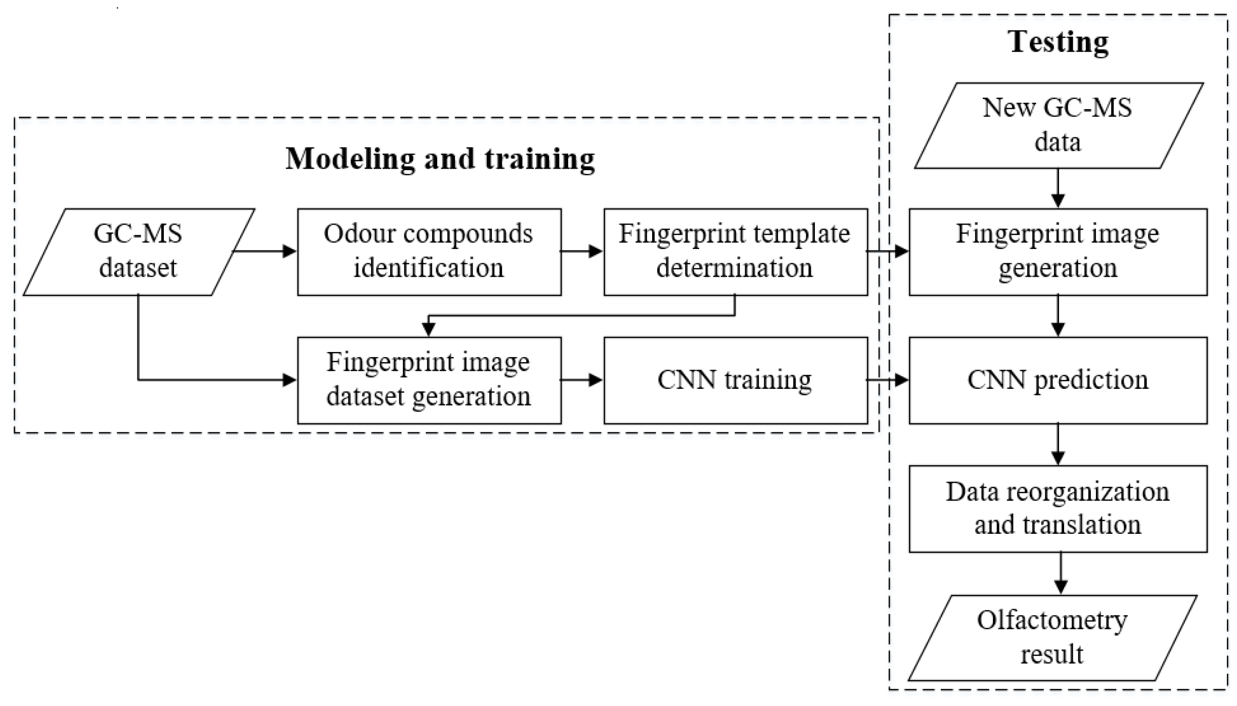
Then using machine-learning methods, data characteristics stored in fingerprint images are extracted for olfactometry results prediction. CNN is applied here as a regression model and the prediction results can be obtained by data reorganization and translation. The process of the whole model is displayed in Figure 1.
3.2. Odor Compound Identification
Odor compounds were identified by their retention indices (RI) and mass spectra, and during the identification, NIST mass spectral library and expert knowledge were applied to determine the specific substance. Modified frequency (MF) [16] was a selection standard for key odor compounds and could be calculated as:
where F (%) is the detection frequency ratio of a specific compound and I (%) is the average intensity expressed as linear percentage of odor intensity rating (0% for 0 and 100% for 4). This index covers the odor compounds information in more detail by combining the intensity and frequency of detection.
For peanut oil samples, the compounds with similar odor type and RT were divided into a same odor group and a total of 20 groups were recorded. The final goal was to obtain the intensity of the 20 odor groups. The detailed identification results can be checked in supplementary files.
3.3. Fingerprint Template Determination
When using NIST mass spectral library, we found that a chromatographic peak could be represented by several compounds with high probability and the selection might be influenced by human factors. To preserve the integrity of analysis information, these compounds should also be considered during prediction. The suitable number of preserved compounds could be five to nine. For each key odor compound in peanut oil, we picked up another six compounds which might be odor compounds or might influence the olfactometry result though they could not be perceived by nose [17] to make a comprehensive consideration of oil differences and avoid human error. Then the number of compounds for the regression was expanded to 375 (a 55 × 7 matrix). The determined odor compounds matrix was named as fingerprint template for peanut oil because the compounds represented the odor characteristics. A piece of fingerprint template of peanut oil is displayed in Figure 2, where all compounds were colored by MF index (the height of the green column represented the MF value) and key compounds were placed in the central column.
A total of seven columns were extracted as shown in the fingerprint template (Figure 2). Column 4 in the middle contained the key odor compounds. Columns 3 and 5 collected carboxylic acids, esters and other compounds that might be a major influence on human sniffing. Columns 2 and 6 selected ketones, aldehydes, alcohols, and other compounds which might make a subordinate contribution to the olfactometry results. Columns 1 and 7 included cyclic compounds, which were released in a low frequency and might prevent correct perceptions the key compounds [18].
For the convenience of programming and explanation of the model, we named the fingerprint compounds template as ‘Matrix C’. Each element C(i,j) represented a specific compound in the template, where i ∊ (1, 2,…, 55) and j ∊ (1, 2,…, 7). As shown in Figure 2, C(1,4) was Hexanal and C(3,2) was 2-Heptanone.
3.4. Fingerprint Image Generation of Each Sample
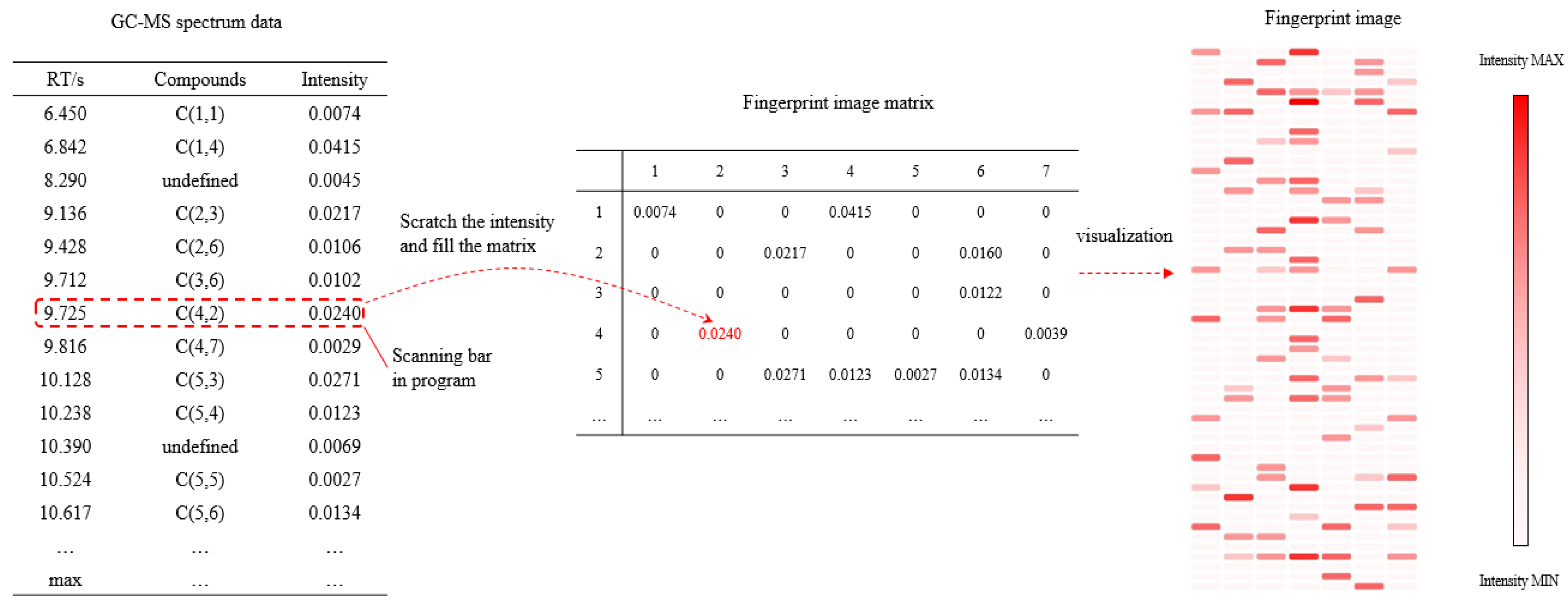
After the confirmation of the fingerprint template, the data structuring process of each GC-MS spectrum was implemented by a computer program. The compound name and normalized peak intensities were extracted from the spectrum and they were sorted by retention time (RT) of each compound. Then the compound names were converted into the elements in Matrix C. If a specific compound did not appear in Matrix C, it would be named as ‘undefined’. This kind of compound sometimes appeared among the volatile compounds in Matrix C. However, they could be filtered out in the model due to the trivial impact on the odor. The computer program defined a sliding scanning bar to read the spectrum from the beginning, and transport the peak intensities into the correct positions in the matrix. This process would break off when the last compound in the spectrum table was read. The mechanism of the program is shown in Figure 3.
Through the fingerprint template (Matrix C) confirmation and fingerprint image generation process, each GC-MS spectrum could be structured into a 55 × 7 matrix with a data format of float number. Then the fingerprint image could be printed by coloring the matrix blank with the intensity value. The shade of the color of each blank indicated the peak intensity of the compounds in the GC-MS spectrum. A fingerprint image of a specific peanut oil sample is displayed on the right side in Figure 3.
3.5. CNN Modeling for Olfactometry Prediction
For peanut oil, the fingerprint image was actually a 55 × 7 matrix which involved the molecular composition characteristics of a specific sample. In addition, the olfactometry result could be converted to a 20-dimentional vector by consulting the odor compounds list, where 20 odor groups were presented. For each olfactometry intensity recorded by sensory evaluation, the RT and odor description were compared to the 20 groups and were filled in the result vector in the proper components. The vector components with no filling value would be set as zero instead. To predict the olfactometry result, a correlation model between the matrix input and the odor vector output should be built up first.
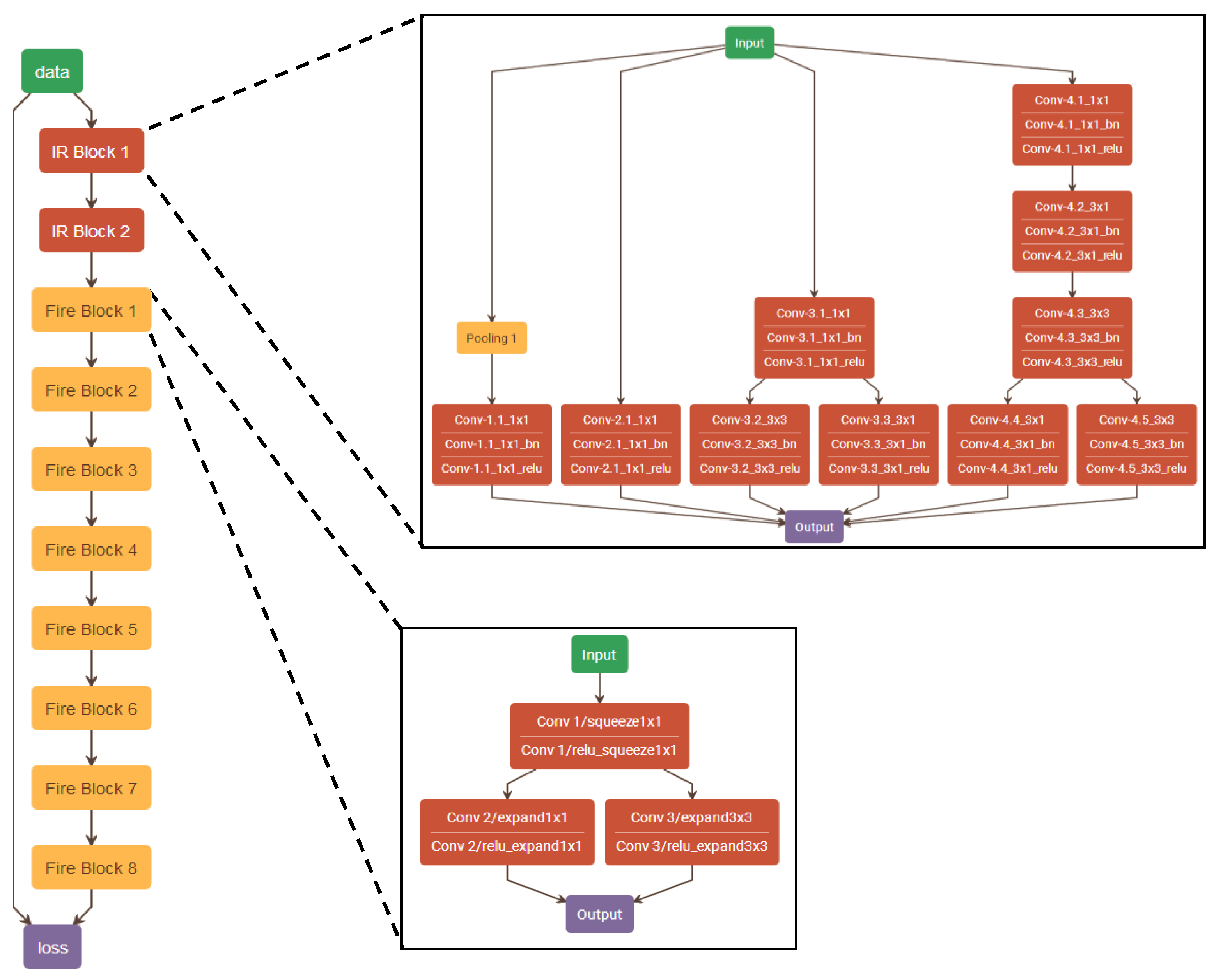
A novel hybrid machine learning model based on CNN was proposed by mixing the structure of GoogLeNet and SqueezeNet [19], as is displayed in Figure 4. This model combined the generalization ability of GoogLeNet and the light-weight design of SqueezeNet, and would undertake feature extraction from the fingerprint then identify the features to make a prediction. IR Blocks represented the GoogLeNet convolution modules, and Fire Blocks represented the SqueezeNet Fire Modules. The specially designed IR Blocks using six convolution kernels of different sizes provide multiple ways to perceive images. The output of the IR blocks concatenated the features extracted by different convolution ways. The Fire Blocks applied 1 × 1 sized kernels to reduce the dimension of the IR blocks output and add more ReLU functions for nonlinear activation of the network. Additionally, the 3 × 3 sized kernels in the Fire Blocks maintained the feature extraction of the network. A total of two IR Blocks and eight Fire Blocks were added into the CNN structure. To reduce overfitting problem, batch normalization [20] and L2 regulation [21] were added in blocks. The detailed convolution operations in these blocks are also introduced in Figure 4.
After obtaining the 20-dimentional odor vector, a computer program found the non-zero vector components and searched the spectrum to determine the odor compound information with a limited range of RT. The prediction process ended with exporting the olfactometry prediction table.
4. Result and Discussion
4.1. Dataset Treatment for CNN Training and Testing
A total of 85 samples of peanut oil bought from supermarkets were analyzed by the GC-MS/O evaluation process. After collecting spectra and generating data as was mentioned above, the dataset was divided into 68 samples (80%) for training and 17 samples (20%) for testing. The division method was based on the ‘train_test_split’ algorithm from the sklearn function library.
4.2. Model Convergence Performance for CNN
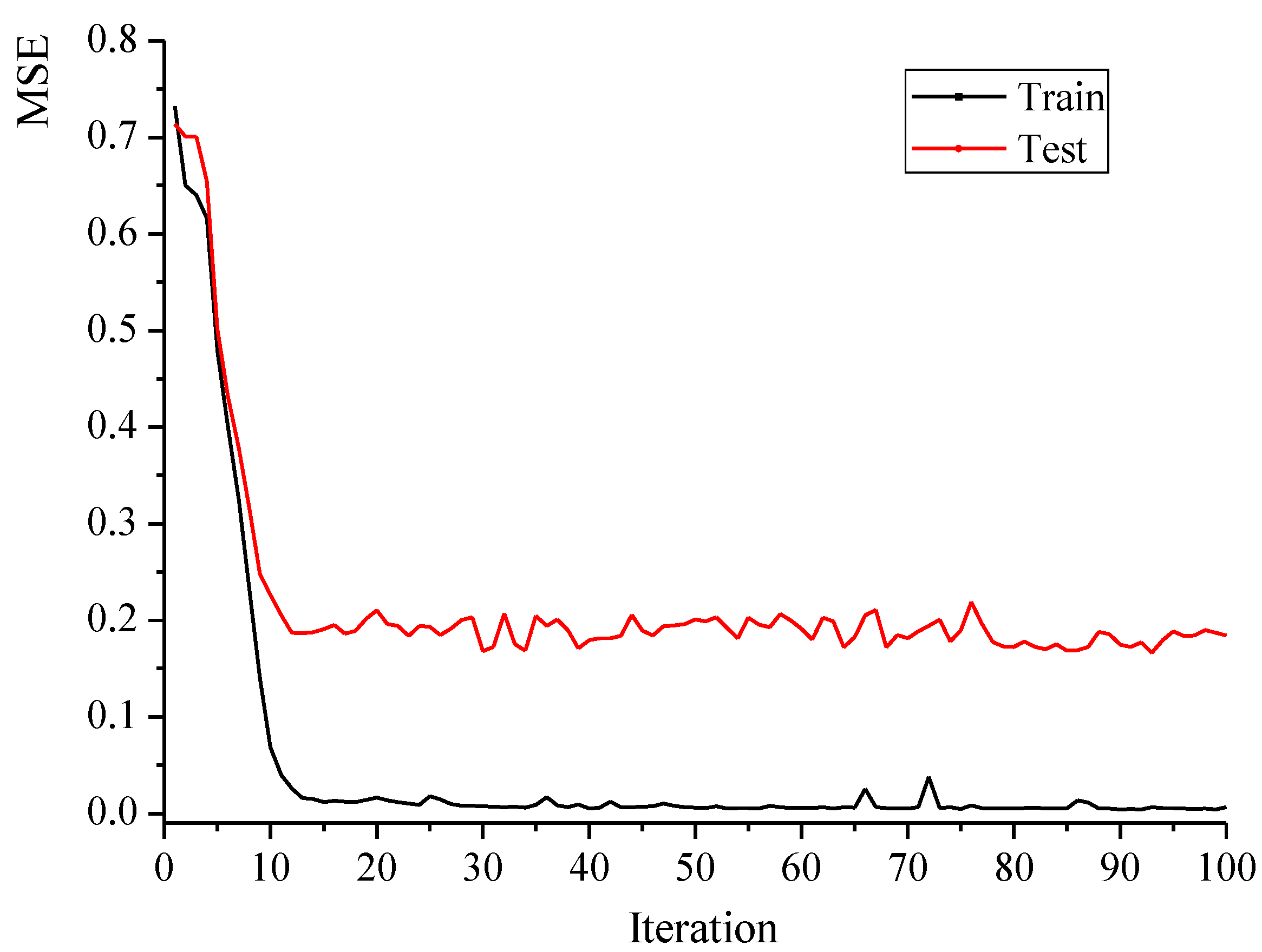
The CNN model was set, as shown in Figure 4, with two IR Blocks and eight Fire Blocks. IR Blocks tried to undertake longitudinal compression to decrease the amount of unnecessary zero elements and enhance the generalization ability of the network. Fire Blocks were sparse regression structures to extract features and convert features to results. Various convolutional operations were executed in this model to provide optic neurons of diverse receptive domain. These optic neurons deciphered the fingerprint through different ways and recorded the information in filters of each blocks’ feature maps. Then the feature maps in the last convolutional block were processed with an average-pooling block to obtain the 20-dimensional odor vector results. The model employed mean square error (MSE) as optimization objective function and Adaptive Moment Estimation (adam) [22] as optimizer. An epoch time of 100 was applied and the fluctuation trend of objective function is plotted in Figure 5. The prediction model was verified to be convergent in about 20 iterations.
4.3. Model Prediction Performance for CNN
The obtained output for validation was a 17 × 20 matrix. To make comparison with actual data, the elements in the matrix were rounded to integers. Three types of judgement might exist during comparison, including correct judgement (predicted value equal to the actual value), intensity deviation (predicted value not equal to the actual value, both not equal to zero), omissive judgement (predicted value not equal to the actual value, predicted value equal to zero), and misdiagnosis (predicted value not equal to the actual value, actual value equal to zero). The detailed comparison result is displayed in Table 1.
As is shown in Table 1, 316 of the total 340 exported odor intensities were identical (error equal to 0) to human olfactometry results, with a correct ratio of 92.94%. Three misdiagnoses (0.88%), nine omissive judgements (2.65%), and 12 intensity deviations (3.53%) resulted in 24 incorrect judgements (7.06%). Among 20 odor groups, Group 12 (nutty, wine), Group 13 (fresh, bean, nutty), and Group 14 (peanut, roasted) owned more than four incorrect judgements, which might be due to the large amount (10 key compounds and over 50 potential odor compounds) of related compounds distributed in the RT range of 19.5–20.4 min (less than 1 min). These compounds’ information were mutual coupling and CNN optic nerves were defective at discriminating them. The concentrated errors might be caused by the insufficient separation ability of GC in this RT range or the excessive volatile compounds selection errors by limited expert knowledge. However, at most two incorrect judgements were detected in the other 17 odor groups and at most three incorrect judgements were detected in all 17 samples, which demonstrated a presentable prediction result.
Besides, an interpretation process was needed to display the human-like olfactometry result. Firstly, zero elements in 20-dimension odor vector should be cut out. Then, the odor of remaining elements was filled by their groups and the approximate RT of each odor group could be detected by searching the corresponding odor compounds’ RT. A final output of a specific peanut oil sample is displayed in Table 2.
4.4. Model Accuracy Comparison with PLSR
A comparison between the widely used PLSR algorithm [23] and the machine learning model was made to verify the practicality of the new method. The same dataset and dataset division method were applied in both processes. A total of 55 key compounds summarized in an odor compounds list were set as the input and the odor intensities of 20 odor groups were set as the output of the PLSR model. The detailed comparison result is shown in Table 3.
Obviously, the new method had a better accuracy in this case study than conventional PLSR model. The CNN model in the new method applied different convolution operations for local feature extraction and nonlinear regression functions, which were efficacious to learn how these odor compounds affected the human sniffing. Besides, the potential issue of an operator or systematic laboratory effect when handling the spectrum data could be decreased by using the convolution kernels in CNN to analyze the compounds of similar RT. While, the PLSR method used linear regression after independent variable selection, which was insufficient for spectrum data mining and was inadequate for feature extraction.
4.5. CNN Structure Design for Sensory Laboratory
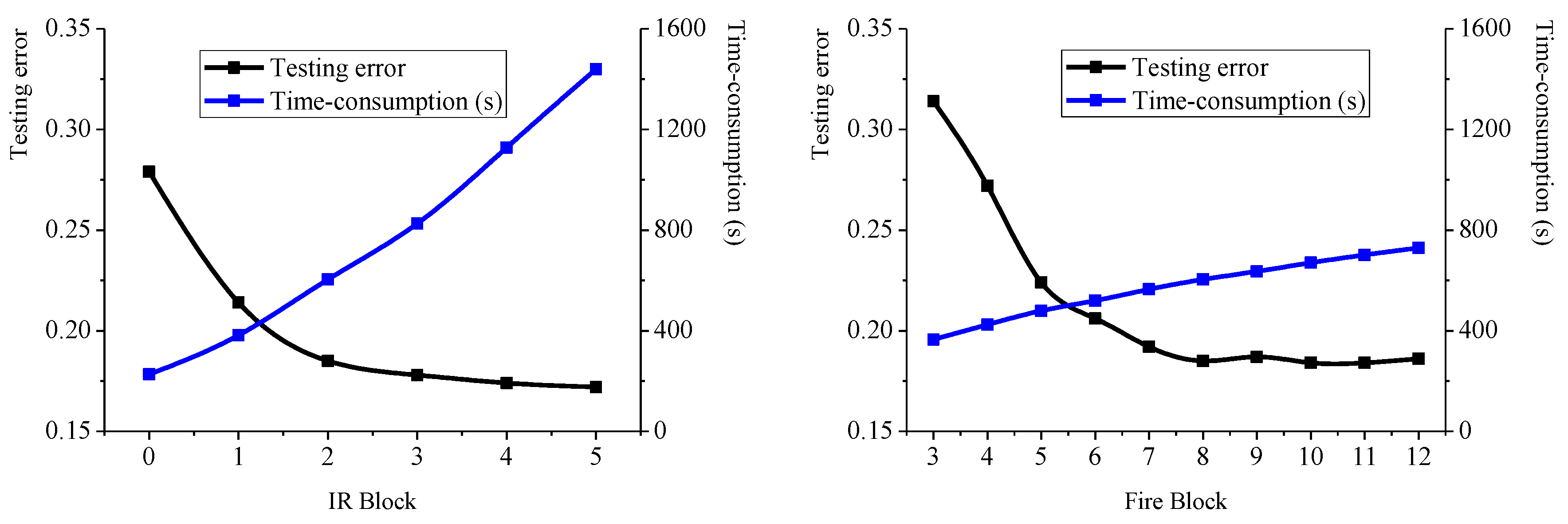
To execute the prediction process in a sensory laboratory, it is essential to balance the accuracy and training time-consumption of the model [24]. Different CNN structures were evaluated to find the optimum depth of the network. These structures were provided with the same training and testing conditions and were evaluated with a same computer (with an Inter core i7-7700HQ CPU @3.8 GHz and a GTX Force 1050Ti GPU @CUDA 9.0, running with python 3.6 using Keras frame [25] on Tensorflow backend). The model performance is shown in Figure 6.
For laboratory use, a structure with an acceptable margin of error and less training time should be selected. Evaluation results in Figure 6 illustrated that two IR Blocks was adequate for feature extraction, because the testing error did not have a sharp decline but the time-consumption for each IR Block was large when the number of blocks reached two. Additionally, eight Fire Blocks was adequate for prediction, because the testing errors levelled off when the number of blocks reached eight. The evolving trend of testing error and the choice of CNN structure can be explained by substructure (blocks) characteristics of the network. IR Blocks based on GoogLenet are designed with excellent generalization performance resulting from its sparse structure and multiple convolution patterns. There are six convolution patterns in a designed IR block, and some patterns consist of multistep convolution. Thus, only a few of these substructures can guarantee the generalization performance and accuracy of the model. Fire Blocks based on Squeezenet are light-weight substructures to obtain regression results with lower-overfitting. Simple convolution patterns make it unfeasible to accomplish the regression task in a limited quantity of substructures, but adding a substructure does not increase the time-consumption too much. Then, eight blocks are added into the CNN structure and a model with acceptable accuracy and time-consumption is obtained.
A CNN structure with about 900,000 parameters, 600 s optimization time-consumption, and 93% accuracy was adopted by the laboratory. After the CNN training (around 600 s) and data structuring of the GC-MS spectrum, the whole process including spectrum profiling, machine learning prediction, and output interpretation could be accomplished within 30 s. As a comparison, a conventional GC-MS/O method employs humans as the sniffing recognizer, generating three to five olfactometry results per person within a working day.
5. Conclusions
A new approach for olfactometry result prediction from GC-MS spectrum data was proposed. The unstructured spectrum data was converted into structured data by fingerprint modeling and then visualized by a fingerprint image. A CNN method was applied to profile the fingerprint image to obtain the olfactometry result. After an overall assessment on peanut oil samples, the novel olfactometry prediction process was demonstrated to be feasible with acceptable accuracy and time-consumption.
Compared to conventional PLSR method, the new approach which combined the design of GoogLenet and SqueezeNet extracted the features with multiple types of convolution kernels in IR blocks and guaranteed the light-weight structure of the model with the sparse Fire Blocks. Besides, the potential issue of an operator or systematic laboratory effect could be decreased by comprehensive utilization of spectrum data and heuristic knowledge.
The structure of CNN was optimized and a model with two IR blocks and eight Fire Blocks was finally selected. After the CNN training (around 600 s) and data structuring of GC-MS spectrum, the whole process including spectrum profiling, machine learning prediction, and output interpretation could be accomplished within 30 s. Although there is still an overfitting problem with the machine learning model, the proposed olfactometry prediction process has potential for a laboratory to complete olfactometry evaluation instead of humans. With the expansion of datasets, the performance of the model could be improved and the overfitting problem could be reduced.
Supplementary Materials
The following are available online at https://0-www-mdpi-com.brum.beds.ac.uk/2227-9717/8/1/23/s1, Table S1: Key compounds in analyzed peanut oil samples.
Author Contributions
Conception and design: K.B., D.Z., T.Q.; Experiment Section: Y.H.; Data collection: K.B., Y.H., D.Z.; Process modeling and optimization: K.B., T.Q.; Establishment of CNN structure: K.B., D.Z., T.Q.; Analysis and interpretation: K.B., T.Q.; Writing the article: K.B., T.Q., Y.H.; Critical revision of the article: K.B., D.Z., T.Q., Y.H.; Final approval of the article: K.B., D.Z., T.Q., Y.H. All authors have read and agree to the published version of the manuscript.
Funding
This research was funded by National Natural Science Foundation of China, Grant No. U1462206.
Conflicts of Interest
The authors declare no conflict of interest.
References
- Dun, Q.; Yao, L.; Deng, Z.; Li, H.; Li, J.; Fan, Y.; Zhang, B. Effects of hot and cold-pressed processes on volatile compounds of peanut oil and corresponding analysis of characteristic flavor components. LWT-Food. Sci. Technol. 2019, 112, 107648. [Google Scholar] [CrossRef]
- Ross, C.F. Sensory science at the human–machine interface. Trends. Food Sci. Tech. 2009, 20, 63–72. [Google Scholar] [CrossRef]
- Plutowska, B.; Wardencki, W. Application of gas chromatography–olfactometry (GC–O) in analysis and quality assessment of alcoholic beverages–A review. Food Chem. 2008, 107, 449–463. [Google Scholar] [CrossRef]
- Delahunty, C.M.; Eyres, G.; Dufour, J.P. Gas chromatography-olfactometry. J. Sep. Sci. 2006, 29, 2107–2125. [Google Scholar] [CrossRef] [PubMed]
- Thomsen, M.; Martin, C.; Mercier, F.; Tournayre, P.; Berdagué, J.L.; Thomas-Danguin, T.; Guichard, E. Investigating semi-hard cheese aroma: Relationship between sensory profiles and gas chromatography-olfactometry data. Int. Dairy J. 2012, 26, 41–49. [Google Scholar] [CrossRef]
- Pang, X.; Guo, X.; Qin, Z.; Yao, Y.; Hu, X.; Wu, J. Identification of aroma-active compounds in Jiashi muskmelon juice by GC-O-MS and OAV calculation. J. Agric. Food Chem. 2012, 60, 4179–4185. [Google Scholar] [CrossRef] [PubMed]
- Brattoli, M.; De Gennaro, G.; De Pinto, V.; Demarinis Loiotile, A.; Lovascio, S.; Penza, M. Odour detection methods: Olfactometry and chemical sensors. Sensors 2011, 11, 5290–5322. [Google Scholar] [CrossRef] [PubMed] [Green Version]
- Szegedy, C.; Liu, W.; Jia, Y.; Sermanet, P.; Reed, S.; Anguelov, D.; Erhan, D.; Venhoucke, V.; Rabinovich, A. Going deeper with convolutions. In Proceedings of the IEEE Conference on Computer Vision and Pattern Recognition, Boston, MA, USA, 7–12 June 2015; pp. 1–9. [Google Scholar]
- He, K.; Zhang, X.; Ren, S.; Sun, J. Deep residual learning for image recognition. In Proceedings of the IEEE Conference on Computer Vision and Pattern Recognition, Las Vegas, NV, USA, 27–30 June 2016; pp. 770–778. [Google Scholar]
- Smirnov, E.A.; Timoshenko, D.M.; Andrianov, S.N. Comparison of regularization methods for imagenet classification with deep convolutional neural networks. AASRI Proc. 2014, 6, 89–94. [Google Scholar] [CrossRef]
- Li, X.; Kong, W.; Shi, W.; Shen, Q. A combination of chemometrics methods and GC–MS for the classification of edible vegetable oils. Chemometr. Intell. Lab. 2016, 155, 145–150. [Google Scholar] [CrossRef]
- Pereira, A.C.; Reis, M.S.; Leça, J.M.; Rodrigues, P.M.; Marques, J.C. Definitive Screening Designs and latent variable modelling for the optimization of solid phase microextraction (SPME): Case study-Quantification of volatile fatty acids in wines. Chemometr. Intell. Lab. 2018, 179, 73–81. [Google Scholar] [CrossRef]
- Scott, D.R. Improved method for estimating molecular weights of volatile organic compounds from low resolution mass spectra. Chemometr. Intell. Lab. 1991, 12, 189–200. [Google Scholar] [CrossRef]
- Keane, P. The flavor profile. In Manual on Descriptive Analysis Testing for Sensory Evaluation; Hootman, R., Ed.; ASTM International: West Conshohocken PA, USA, 1992; pp. 5–14. [Google Scholar]
- Esteki, M.; Farajmand, B.; Amanifar, S.; Barkhordari, R.; Ahadiyan, Z.; Dashtaki, E.; Mohammadlou, M.; Vander Heyden, Y. Classification and authentication of Iranian walnuts according to their geographical origin based on gas chromatographic fatty acid fingerprint analysis using pattern recognition methods. Chemometr. Intell. Lab. 2017, 171, 251–258. [Google Scholar] [CrossRef]
- Dravnieks, A. Atlas of odor character profiles. In Manual on Descriptive Analysis Testing for Sensory Evaluation; Hootman, R., Ed.; ASTM International: West Conshohocken PA, USA, 1992; pp. 354–355. [Google Scholar]
- Delwiche, J. The impact of perceptual interactions on perceived flavor. Food Qual. Prefer. 2004, 15, 137–146. [Google Scholar] [CrossRef]
- Frank, D.C.; Owen, C.M.; Patterson, J. Solid phase microextraction (SPME) combined with gas-chromatography and olfactometry-mass spectrometry for characterization of cheese aroma compounds. LWT-Food. Sci. Technol. 2004, 37, 139–154. [Google Scholar] [CrossRef]
- Iandola, F.N.; Han, S.; Moskewicz, M.W.; Ashraf, K.; Dally, W.J.; Keutzer, K. SqueezeNet: AlexNet-level accuracy with 50x fewer parameters and<0.5 MB model size. arXiv 2016, preprint. arXiv:1602.07360. [Google Scholar]
- Ioffe, S.; Szegedy, C. Batch normalization: Accelerating deep network training by reducing internal covariate shift. arXiv 2016, preprint. arXiv:1502.03167. [Google Scholar]
- Cortes, C.; Mohri, M.; Rostamizadeh, A. L2 regularization for learning kernels. In Proceedings of the Twenty-Fifth Conference on Uncertainty in Artificial Intelligence, Montreal, QC, Canada, 18 – 21 June 2009; pp. 109–116. [Google Scholar]
- Kingma, D.P.; Ba, J. Adam: A method for stochastic optimization. arXiv 2014, preprint. arXiv:1412.6980. [Google Scholar]
- Wold, S.; Sjöström, M.; Eriksson, L. PLS-regression: A basic tool of chemometrics. Chemometr. Intell. Lab. 2001, 58, 109–130. [Google Scholar] [CrossRef]
- Wu, J.; Leng, C.; Wang, Y.; Hu, Q.; Cheng, J. Quantized convolutional neural networks for mobile devices. In Proceedings of the IEEE Conference on Computer Vision and Pattern Recognition, Las Vegas, NV, USA, 27–30 June 2016; pp. 4820–4828. [Google Scholar]
- Ketkar, N. Introduction to keras. In Deep Learning with Python; Ketkar, N., Ed.; Apress: Berkeley, CA, USA, 2017; pp. 97–111. [Google Scholar]
Figure 1.
Olfactometry prediction process of food product using gas chromatography-mass spectrometry (GC-MS) data.
Figure 1.
Olfactometry prediction process of food product using gas chromatography-mass spectrometry (GC-MS) data.

Figure 2.
A piece of the fingerprint compounds template (55 × 7) colored by modified frequency (MF).
Figure 2.
A piece of the fingerprint compounds template (55 × 7) colored by modified frequency (MF).

Figure 3.
The process of fingerprint image generation by computer program.

Figure 4.
Convolutional neural network (CNN) model structure applied in prediction model.

Figure 5.
The fluctuation trend of objective function during CNN training.

Figure 6.
The model performance as a function of block numbers.


Table 1.
The detailed comparison results of the olfactometry forecasting.
| Group | 1 | 2 | 3 | 4 | 5 | 6 | 7 | 8 | 9 | 10 | 11 | 12 | 13 | 14 | 15 | 16 | 17 | 18 | 19 | 20 |
| 1 |  | | | |  | | | | | | | | | | | | | | | |
| 2 | | | | | | | | | | | | |  | | | | | | | |
| 3 | | | | | | | | | | | |  | | | | | | | | |
| 4 | | | | | | | | | | | | | | | | | | | | |
| 5 | | | | | | | | | | | | | | | | | | | | |
| 6 | | | | | | | | | | | | | | | | | | | | |
| 7 | | | | | | | | | | | | | | | | | | | | |
| 8 | | | | | | | | | | | | | | | | | | | | |
| 9 | | | | | | | | | | | | | | | | | | | | |
| 10 | | | | | | | | | | | | | | | | | | | | |
| 11 | | | | | | | | | | | | | | | | | | | | |
| 12 | | | | | | | | | | | | | | | | | | | | |
| 13 | | | | | | | | | | | | | | | | | | | | |
| 14 | | | | | | | | | | | | | | | | | | | | |
| 15 | | | | | | | | | | | | | | | | | | | | |
| 16 | | | | | | | | | | | | | | | | | | | | |
| 17 | | | | | | | | | | | | | | | | | | | | |
Correct judgement Intensity deviation Omissive judgement Misdiagnosis.Table 2.
The detailed comparison results of the olfactometry forecasting.
| RT/min | 6.65 | 10.56 | 10.93 | 14.05 | 19.56 | 20.93 |
| Odor | Grass | Rubber, hazelnut | Nutty, roasted | Mushroom | Nutty, wine | Peanut, roasted |
| Intensity | 2 | 2 | 1 | 2 | 2 | 2 |
Table 3.
The overall accuracy comparison of two methods.
| Overall Ratio | Correct Judgement | Intensity Deviation | Omissive Judgement | Misdiagnosis |
|---|---|---|---|---|
| New Method | 92.9% | 3.5% | 2.6% | 0.9% |
| PLSR | 66.8% | 16.8% | 10.6% | 5.9% |
© 2019 by the authors. Licensee MDPI, Basel, Switzerland. This article is an open access article distributed under the terms and conditions of the Creative Commons Attribution (CC BY) license (http://creativecommons.org/licenses/by/4.0/).
Share and Cite
MDPI and ACS Style
Bi, K.; Zhang, D.; Qiu, T.; Huang, Y. GC-MS Fingerprints Profiling Using Machine Learning Models for Food Flavor Prediction. Processes 2020, 8, 23. https://0-doi-org.brum.beds.ac.uk/10.3390/pr8010023
AMA Style
Bi K, Zhang D, Qiu T, Huang Y. GC-MS Fingerprints Profiling Using Machine Learning Models for Food Flavor Prediction. Processes. 2020; 8(1):23. https://0-doi-org.brum.beds.ac.uk/10.3390/pr8010023
Chicago/Turabian StyleBi, Kexin, Dong Zhang, Tong Qiu, and Yizhen Huang. 2020. "GC-MS Fingerprints Profiling Using Machine Learning Models for Food Flavor Prediction" Processes 8, no. 1: 23. https://0-doi-org.brum.beds.ac.uk/10.3390/pr8010023
Note that from the first issue of 2016, this journal uses article numbers instead of page numbers. See further details here.