Triple-Mode Model Predictive Control Using Future Target Information


National Center for International Research on Quality-Targeted Process Optimization and Control, College of Control Science and Engineering, Zhejiang University, Hangzhou 310027, China
*
Author to whom correspondence should be addressed.
Processes 2020, 8(1), 54; https://0-doi-org.brum.beds.ac.uk/10.3390/pr8010054
Submission received: 9 December 2019
/
Revised: 27 December 2019
/
Accepted: 30 December 2019
/
Published: 2 January 2020
(This article belongs to the Special Issue Process Optimization and Control)
Abstract
:In this paper, we propose a triple-mode model predictive control (MPC) algorithm that uses future target information to improve tracking performance. To explicitly take into account the future target information in the MPC optimization, the proposed triple-mode control law encompasses three parts: (i) the future target information feedforward, (ii) the output feedback, and (iii) the extra degrees of freedom for constraint satisfaction. The first two parts of the control law are off-line designed through unconstrained MPC, and the optimal future trajectory horizon is obtained by golden section search based on the integral of squared error (ISE) criterion. The final part is calculated by the on-line MPC algorithm aiming to satisfy constraints. Furthermore, we analyze the feasibility and convergence properties of the proposed algorithm. The method is demonstrated by the simulation of the shell fundamental control problem and also tested on the coordinated control problem in the power plant. The test results show that the proposed algorithm can increase tracking performance dramatically due to the proper selection of future trajectory horizon.
1. Introduction
Concern about multivariable constrained system control has become a central issue in the control domain. As a result, much research in recent years has focused on the development of advanced control algorithms that are process friendly. Model predictive control (MPC) has been widely and successfully applied in the process industry, primarily due to its superior performance and the capability of dealing with a multivariate constrained problem [1,2,3]. Since the step-response model is more convenient to obtain and more suitable for the process industry, this model has been successfully applied to numerous industrial processes by Aspen Technology, Honeywell Hi-Spec, and others. There has been an increase in the adoption of dynamic matrix control in MPC commercial software packages such as DMC+, SMC, RMPCT, HIECON [1].
The key idea of model predictive control is to use the historical information and model prediction to calculate the optimal input trajectory by minimizing the deviation between the process output and the desired target in a receding horizon way. There exists a rich supporting theory [4,5,6] for its success in industry. Moreover, the applications of model predictive control have already gone beyond petrochemical or chemical industries and extended to power plants [7], traffic, robots [8] and any other fields.
The research to date has tended to focus on the regulation problem (steer the system to the origin) [4] for facilitating the analysis and design. The regulation problem assumes the hypothesis that the future setpoint is fixed or changes instantaneously, thus future target information is rarely discussed in the current literature. Considering the setpoint changes, Limón et al. [9] adopted a modified cost function and a stabilizing extended terminal constraint in MPC optimization to obtain the feasible setpoints in case that the setpoints are not feasible. Their work is still preserving no consideration of using the future target information. The MPC optimization have the capability of considering the future target information [10], which may be helpful in control since it allows the controller to react to the setpoint changes in advance [11]. Carrasco and Goodwin [12] proposed a feedforward model predictive control, in which the feedforward was designed individually before the feedback design. However, how much future target information (so-called “preview” in their work) should be used in feedforward design is not discussed in their work. Rossiter and Grinnell [13] developed an extended input horizon generalized predictive controller (EIHGPC) algorithm, in which they parameterized the degrees of freedom to spread the control increments over the prediction horizon and adopted a heuristic algorithm to select a proper future target horizon, hence improves the tracking performance. Their method only pertains to the unconstrained case. In [14], the authors proposed a dual-mode constrained MPC algorithm, which was composed of a linear state feedback and extra degrees of freedom. Under such a control law, the feedforward could not be designed individually and the future target horizon was determined through a trial and error process.
However, the inappropriate use of future target information may cause the deterioration of control performance [13,15]. There remains a need for an effective method that can determine a proper future target horizon. Moreover, the current implementations of MPC fail to separately design the feedforward, feedback and constraint satisfaction, which could not yield the desirable performance from each part. In this study, a triple-mode constrained model predictive control algorithm is developed, which has the merit of independent design for each mode of the control law. The main ingredients of the triple-mode control law are: (i) the feedforward design using future target information, (ii) the output feedback, and (iii) the extra degrees of freedom for constraint satisfaction. In addition, a golden section search method is proposed to optimize the future trajectory horizon, which can be used to design the feedforward to improve the tracking performance.
The outline of this article is as follows. First, we describe the typical dynamic matrix control. Next, we give the future target information feedforward structure derived from the unconstrained control law and propose an optimization method for the selection of future trajectory horizon. We then introduce the triple-mode model predictive control using future target information. Finally, we provide two illustrative simulation examples.
2. Preliminary
Mathematical notations used throughout this paper are defined as follows. Given a vector , the symbol denotes the Euclidean 2-norm and denotes the quadratic form of x. e.g., ; denotes the transpose of A; Given two integers, , we define the set . The superscript ∗ denotes the optimal solution or cost according to the context.
Dynamic Matrix Control Algorithm
The design of the MPC algorithm in this paper follows the standard DMC approach proposed by Garcia and Morshedi [2]. Without loss of generality, we consider a MIMO linear dynamic system with controlled variables and manipulated variables. The DMC algorithm adopts a non-parametric step response model as the predictor, thus the ith output at time t can be formulated by the following step response model
in which denotes the jth input increment, i.e., . denotes the kth element of the corresponding step response, and the step response sequence of the ith output to the jth input is . For a stable plant this sequence will asymptotically reach a constant value, i.e., , ().
Based on the step response model, the output predictions over n future steps can be expressed as follows
where
is a vector of the future control moves at time t. is the dynamic states of the system, and is the future output vector at time assuming the input remain constant starting at time , which means for . The evolution of predictions can be obtained by translation of one-step prediction plus the contribution made by the latest control move .
To achieve the goal of offset-free tracking, a bias is introduced into the model to incorporate the feedback. It’s assumed that the model prediction and the measured output at the current time is due to a constant step disturbance at the output. The constant output step disturbance assumption is standard in industrial applications [16]. The model bias is based on the latest output measurement and the predicted outputs
in which refers to the prediction of output at time t based on the measurements up to time . The bias is added to compensate the output prediction
where denotes the estimate of at time t before the latest measurements are obtained. is the revised estimate of on the basis of the feedback, and refers to the weighting matrix of the bias term.
For open-loop stable systems, the future control moves over the control horizon (M) is optimized to drive the model predicted outputs as closely as possible to a desired future trajectory over prediction horizon (P). The DMC optimization problem is defined as
where are input constraints and increment constraints, respectively. The matrix is the dynamic matrix with block matrix and is the shift matrix with appropriate dimension. are the weighting matrices for outputs and the controller moves. The above notations read
At every sample time, controller evaluates its future input trajectories by solving the optimization problem (5) and sends the first step of its entire future input trajectory to its actuators. However, although the future target information of the controlled variable were embedded in the optimization problem of DMC algorithm, the default choice in DMC algorithm was . Little attention has been paid to the selection of an appropriate future trajectory horizon and the use of future target information.
3. Main Results
In this section, we first derive the explicit control law of the unconstrained MPC, which includes two parts: (i) the future target information feedforward, and (ii) the output feedback. Based on the future target information feedforward, we demonstrate that a poor future trajectory horizon has quite an impact on the system’s performance. Then we propose an optimization method to determine the future trajectory horizon and the tripe-mode model predictive control using future target information. The triple-mode MPC is composed of the designed unconstrained control law and the extra degrees of freedom. The future target information is taken into account explicitly to improve tracking performance.
3.1. Illustrations of Poor Future Trajectory Horizon
Now we show that the unconstrained MPC control law will provide possibilities in the explicit expression of feedforward and feedback. Consider the performance objective in problem (5), one can derive the unconstrained law by minimizing it w.r.t the future control moves, according the extremum condition , we have
and making the following substitutions
then we can get
It can be seen that the future target information is involved in the first term of the control law: , which can be seen as the feedforward in the unconstrained control law. In addition, the second part of the control law can be seen as the output feedback based on the current output prediction.
For convenience, we define the future trajectory horizon in feedforward term for each output as , which indicates the length of future target information considered in the optimization. Any future targets beyond the future trajectory horizon will not be taken into account in the optimization problem, even if known. For a given , the future target information adopted in MPC can be expressed as
Furthermore, by combining the specific future trajectory horizon, the unconstrained law can be represented as follows:
where refers to the ith feedforward contribution, and is the reconstructed future target information feedforward component based on the designed future trajectory horizon .
and denotes the jth column vector of the feedforward matrix .
It indicates that, for the ith output, the original P-dimension target vector has been replaced by a designed -dimension vector . A major current focus in improving the control performance is how to select a proper . It is known that the typical DMC algorithm considers no setpoint changes during the optimizaiton, which is equivalent to set the future trajectory horizon as .
Next, we examine the closed-loop performances of the MPC algorithm adopting different choices of future trajectory horizon. Consider a single-input, single-output system described by the following transfer function
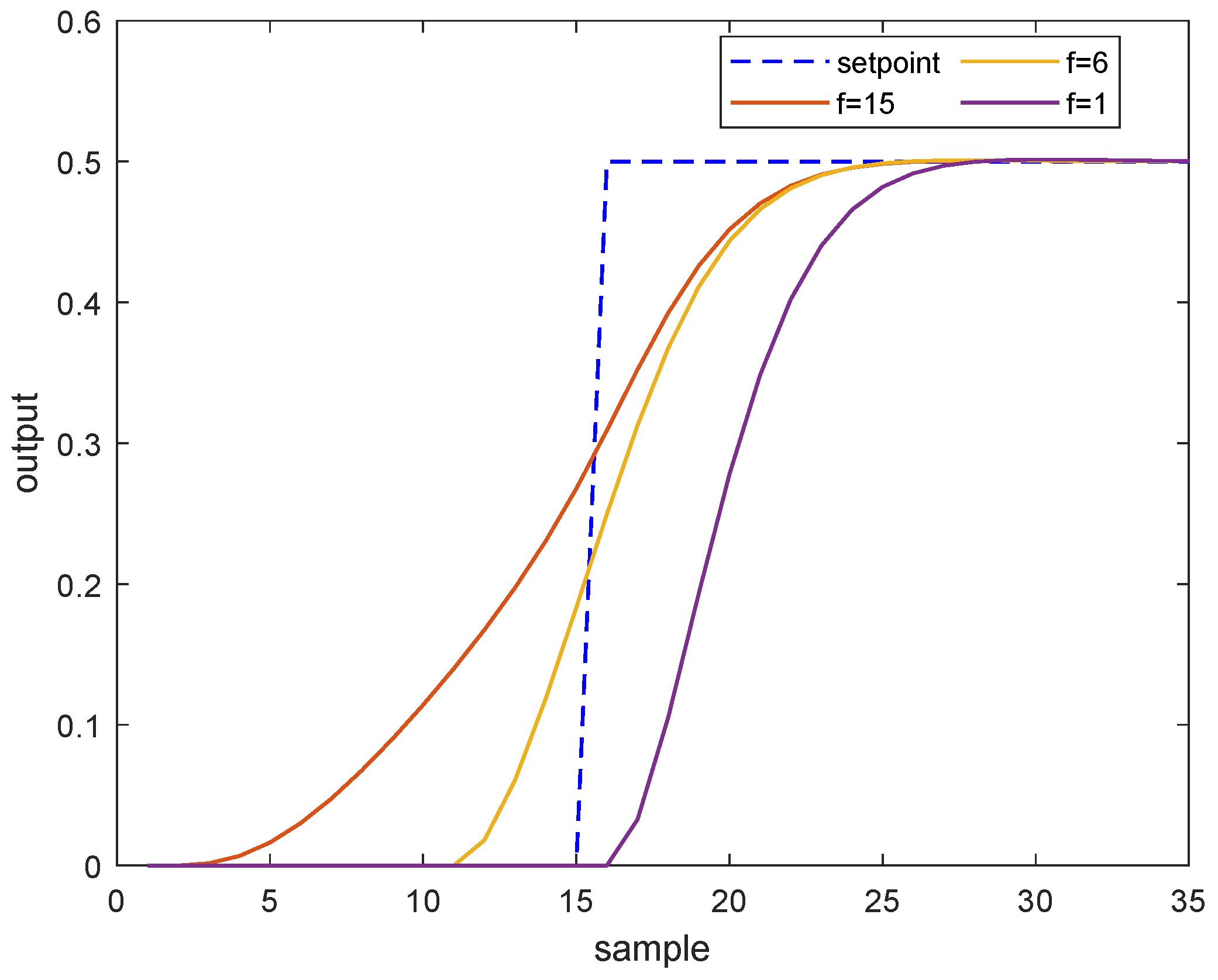
The sampling time is chosen as 5 s, a step change of setpoint happens at sampling instant 15 and the unconstrained MPC algorithm is applied to drive the system to its target. The arbitrary choices of future trajectory horizon are . The tuning parameters of DMC are: and in which I is the identity matrix.
As illustrated by Figure 1, with a default choice of future trajectory horizon in MPC (), the system response is slugglish when the setpoint changes, in contrast, setting the future trajectory horizon as the prediction horizon could result in an aggressive response. A proper selection deserves a desirable tracking performance.
The integral of squared error (ISE) criterion is widely used to evaluate the system performance in control engineering, the discrete form of ISE reads
in which refers to the difference between the expected value (target value) and the actual response value at time instant t.
The ISE values shown in Table 1 demonstrate that the standard MPC algorithm with no anticipation () owns large ISE value during the transition from one target to another. On the other hand, with large number of future trajectory horizon (), the system would react far in advance and lead to bad performance too.
3.2. Future Trajectory Horizon Optimization Algorithm
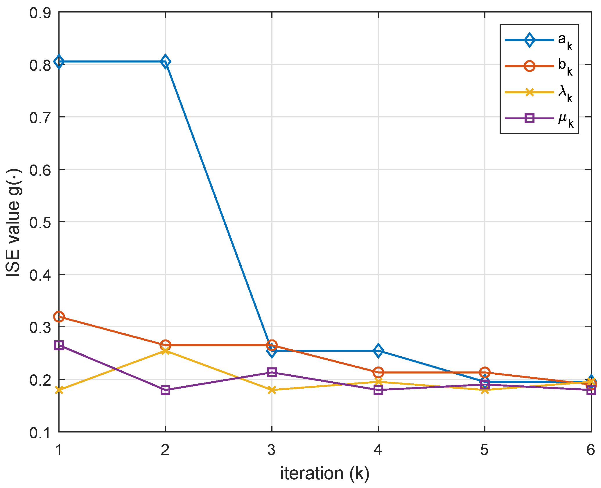
Since the closed-loop response with smaller ISE value is better, we advocate use of the ISE value to select the proper future trajectory horizon. The ISE value can be regarded as a function of future trajectory horizon, i.e., . A better deserves lower function value , we take the idea of golden section search algorithm [17] to optimize the future trajectory horizon. The algorithm can be summarized as follows:
According to Algorithm 1, we plot the ISE value subject to the iteration of as Figure 2 shows. The optimal future trajectory horzion obtained is . Which testifies the result of last section.
| Algorithm 1: The optimization of Future trajectory horizon based on ISE value |
|
3.3. Triple-Mode MPC Algorithm Using Future Target Information
For the conventional MPC algorithm, the optimization problem (5) is solved with degree of freedom to tackle constraints. However, the original optimization problem treats the input as decision variables, which breaks down the inherent future target information feedforward structure as described before. What’s more, the default choice of future trajectory horizon in the MPC algorithm may lead to sluggish tracking performance. There exists no effective method to determine a proper future target horizon for MPC optimization.
With the proposed Algorithm 1 used, we next present a triple-mode MPC algorithm using future target information. Different from the typical DMC algorithm as described in preliminary section, the proposed triple-mode control law encompasses three parts: (i) the future target information feedforward, (ii) the output feedback, and (iii) the extra degrees of freedom. Each mode of the control law can be designed individually. The first two parts of the control law are off-line designed through unconstrained MPC, and the optimal future trajectory horizon is obtained by using Algorithm 1. The final part is calculated by the on-line MPC algorithm aiming to satisfy constraints.
Enhance the unconstrained MPC control law Equation (8) with an additional term
in which and representing degrees of freedom to get the constraints satisfied.
It indicates that the original degree of freedom in constrained DMC optimization (5) is replaced by , which not only provide the feedforward design from future target information but also guarantee the advantage of constraint satisfaction. At each sampling time, the controller solves the following optimization problem
where Equation (17f) refers to the terminal constraint used to ensure closed-loop stability when model predictive control is employed. After optimization, the optimal solution can be obtained, and the optimal input increment is nothing but with . Note that the proposed triple-mode MPC optimiazation problem (17) is a quadratic programming [18] with degrees of freedom. The degrees of freedom are the same as the original DMC optimization problem (5), thus the computation load of proposed triple-mode MPC is the same as which of DMC.
A detailed implementation procedure of the proposed triple-mode MPC algorithm (Algorithm 2) is summarized as follows.
| Algorithm 2: Triple-mode MPC algorithm using future target information |
|
In this section, the triple-mode MPC using future target information is presented. As has been previously stated, this triple-mode control law is based on the usage of the perturbations on the fixed dual-mode unconstrained control law. To this end, the following assumption is considered.
Assumption A1.
The step response sequenceis a Cauchy sequence:.
Assumption A2.
The weighting matricesandare positive definite matrices. At least as many inputs as outputs is required:.
The future target is admissible if there exist a set of control sequence such that the system output can reach it and the constraints (e.g., ) can be satisfied during the stage. The following theorem follows immediately.
Theorem 1.
Consider that Assumption 1 and 2 hold, and the future target is admissible. Then, for any feasible initial state , the proposed triple-mode controller asymptotically steers the system to .
The proof can be found in the Appendix A.
4. Applications
In this section, dynamic simulations are carried out to evaluate the performance of the proposed triple-mode controllers. This section presents two illustrative applications for the proposed methodology: (i) the shell fundamental control problem (case study I), and (ii) the coordinated control problem in the power plants (case study II). We aim at showing the better performance can be achieved by proper selection of future trajectory horizon. The simulation case study was performed on a PC with Intel Core i5 Quad 1.6GHz, 16GB memory and in the Matlab platform.
4.1. System I: A Heavy Oil Fractionator
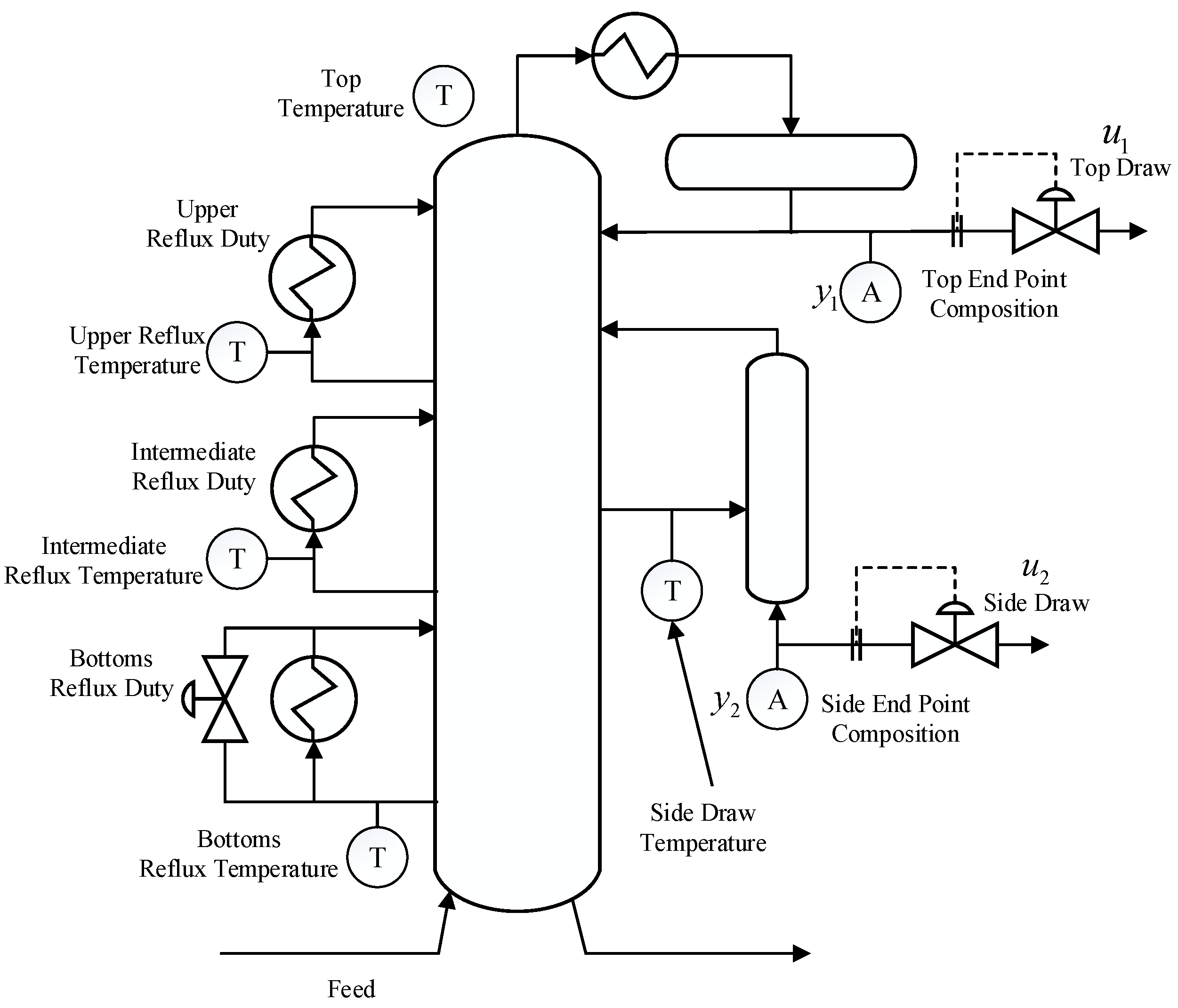
In this example, consider a plant shown in Figure 3 presented in Prett and Morari [19]. in which a gaseous feed stream is separated by removing heat.
Here we will only consider the two-by-two subsystem, which consists of two inputs: the top draw and the side draw ; two outputs: the top end point and the side end point . The model for this system is:
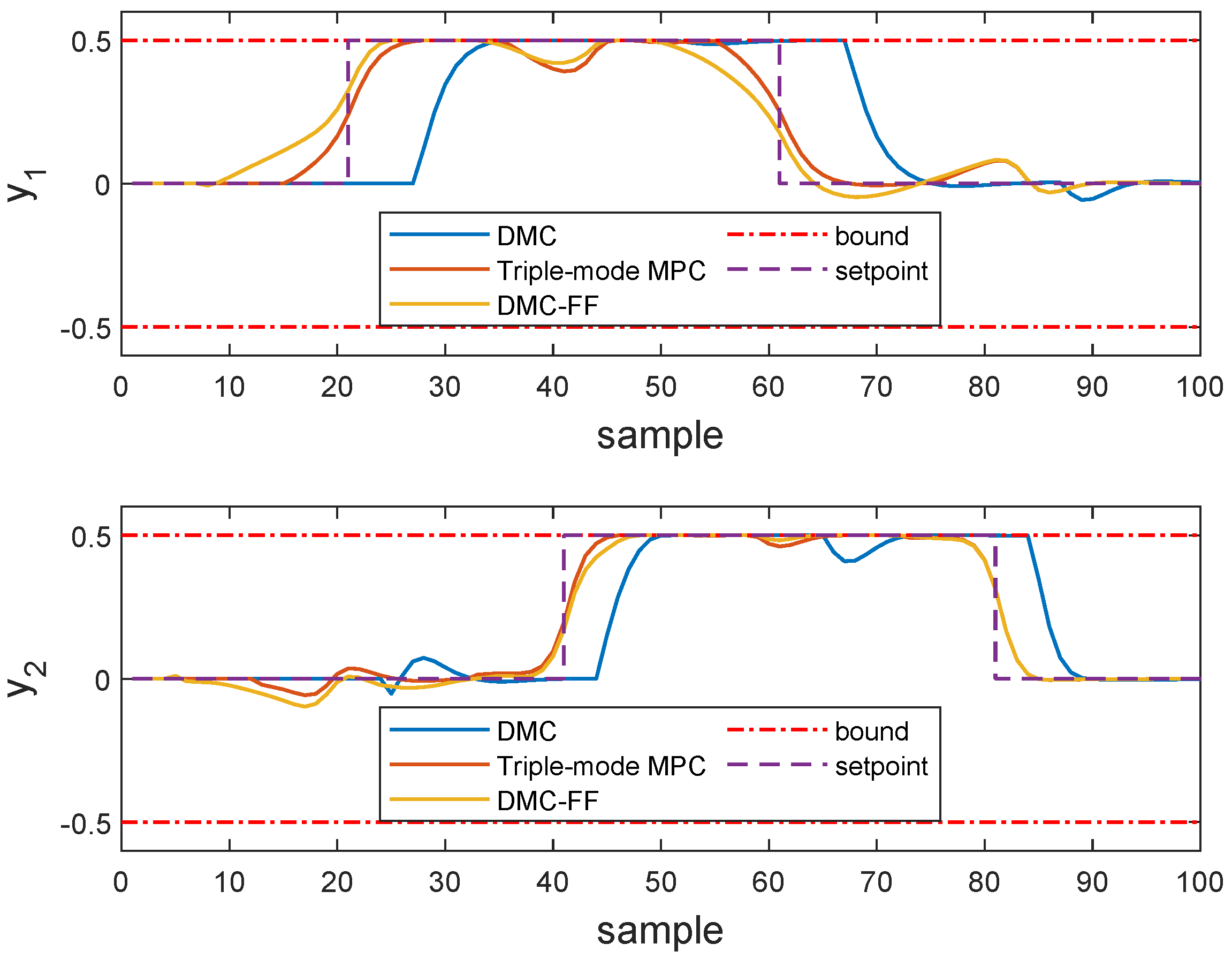
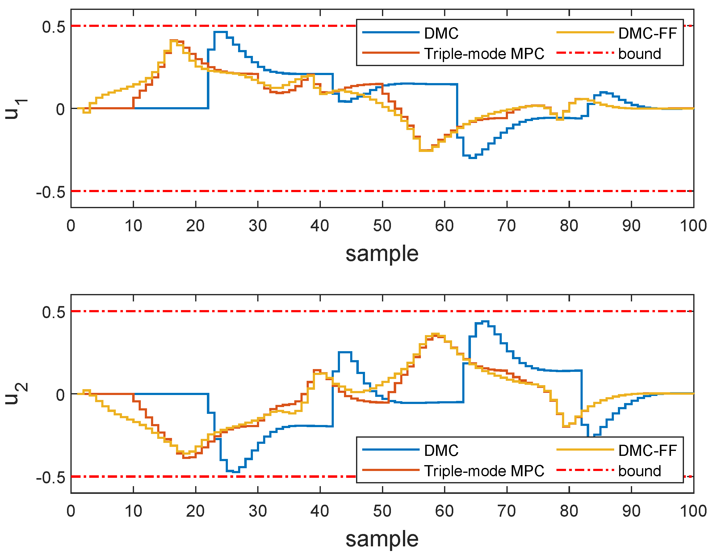
The system will be represented using a 60-coefficient step response model with a 5-min sampling time. Set the initial operating point to be the origin and the upper bound of both output and input is , the lower bound of both output and input is . Three MPC algorithms are used to compare the system performance: the typical DMC, the proposed triple-mode MPC (Algorithm 2), and the DMC algorithm with an artificial selection of future target horizon (denoted as DMC-FF in the following). Tuning parameters of the MPC controllers are the same as follows: a prediction horizon of and a control horizon of . The weighting matrices are set as identity matrix. In the DMC-FF algorithm, the future target horizon is selected as . In the triple-mode MPC algorithm, the optimal future target horizon can be obtained as according to Algorithm 1. To compare the tracking performance, the evolution of setpoint is given as: the initial setpoint is coincident with the system’s initial operating point; at sample time 20, change the setpoint of output to its upper bound and the setpoint of output is also changed to its upper bound when sample time 40; at sample time 60, set the setpoint of output to the origin and the setpoint of output is also set to the origin at sample time 80.
As it can be seen in Figure 4, both two outputs are sluggish under the typical DMC algorithm when the setpoint changed. On the other hand, using an artificial selection of future target horizon may cause the system to response to the future target information far in advance. The performance is degraded because the typical DMC algorithm overlooks the information of future target and the DMC-FF algorithm uses too much future target information. In contrast, the triple-mode MPC algorithm which taking into account the future target information properly can respond to subtlety, the performance of the system is improved dramatically.
Next, Table 2 shows the sum of the ISE value of the controlled system for each control strategy throughout the simulation horizon. The DMC-FF using the future target information can outperform the typical DMC, and the triple-mode MPC using an optimal future target horizon achieves the best tracking performance among the three algorithms.
4.2. System II: A Power Plant Coordinated Control System
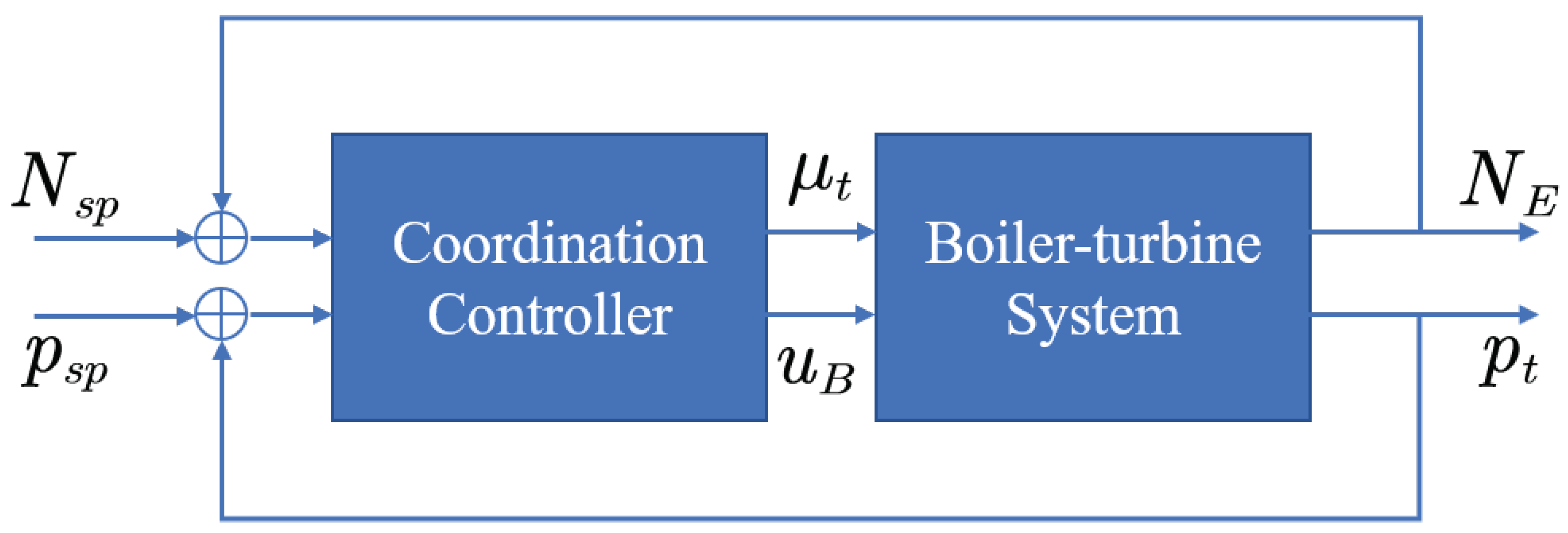
Coordinated control system (CCS) is the system that coordinates the steam turbine and the boiler at the same time to respond to the various load demands quickly [20]. The boiler and the turbine possess different dynamic characteristics. The dynamic from the combustion rate to the main steam pressure is a slow process with large delay and great inertia. In contrast, the response from the turbine governor valve to the unit output is a relatively fast process.
The simplified coordinated control system can be shown in Figure 6.
It can be seen that this system is a two-input, two-output control system, in which the manipulated variables are the fuel command and the opening level of the turbine valve , the controlled variables are the main steam pressure and the output power . Consider a unit in Datang Panshan Power Plant, China, in which the CCS is composed of the boiler of Type boiler and the turbine of Type . The nonlinear model from the load to load was identified through the step test [21]. When the load , the linearized model is:
In this case study, it was established that the control system must always obey the speed restriction on the manipulated variables , and the system is initially at = 550 MW, = 16.9 Mpa. The sampling time is s. Three MPC algorithms are used to compare the system performance: the typical DMC, the proposed triple-mode MPC (Algorithm 2), and the DMC algorithm with an artificial selection of future target horizon (denoted as DMC-FF in the following). Tuning parameters of the three MPC algorithms are the same as follows: the prediction horizon is and the control horizon is ; the weighting matrices are set as: the weight for is and for is , the weight for inputs is . In the DMC-FF algorithm, the future trajectory horizon for outputs and are set to respectively. In addition, the triple-mode MPC adopts to design the feedforward based on Algorithm 1. The main purpose of the CCS is to keep the output power responding to load demands quickly when the unit running in either constant or sliding pressure operation. The following two scenarios are considered:
4.2.1. Constant Pressure Operation
When the unit is running in constant pressure operation mode, the main steam pressure is maintained at the rated value regardless of any changes in load demand.
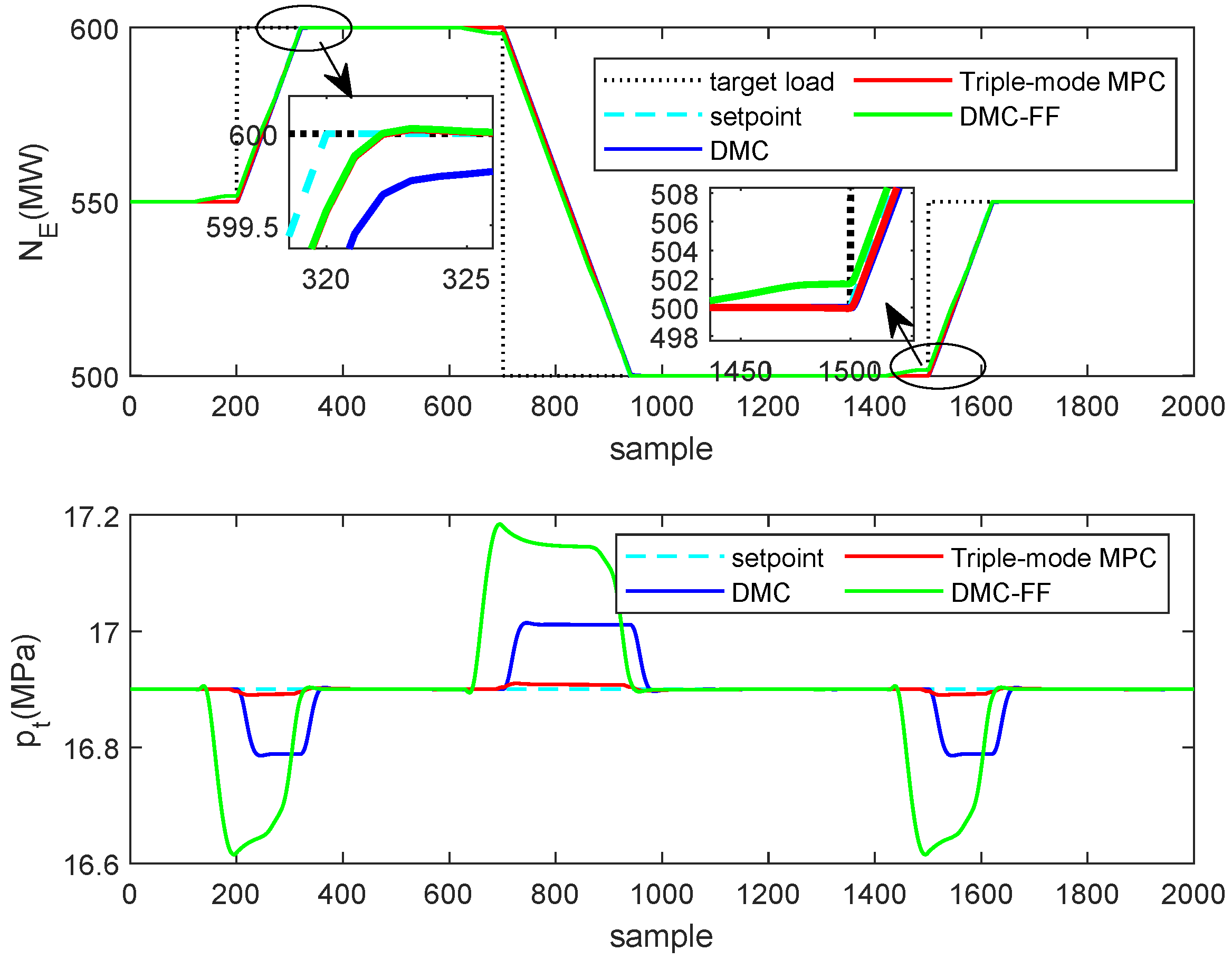
Assuming that the evolution of load demand is given as: the initial load demand is coincident with the system’s initial operating point MW; at sample time 200, change the load demand to 600 MW then remain constant; at sample time 700, set the target load to 500 MW and then push it to the 550 MW at time instant 1500. In order to prevent the step load disturbance of the target load from impacting the entire control system of the unit, the setpoint of the output power is formed by limiting the load change rate after the target load is changed [22]. In general, the load change rate is determined by the operating personnel according to the operating conditions of the unit equipment. Here we set the load change rate as 5 MW/min.
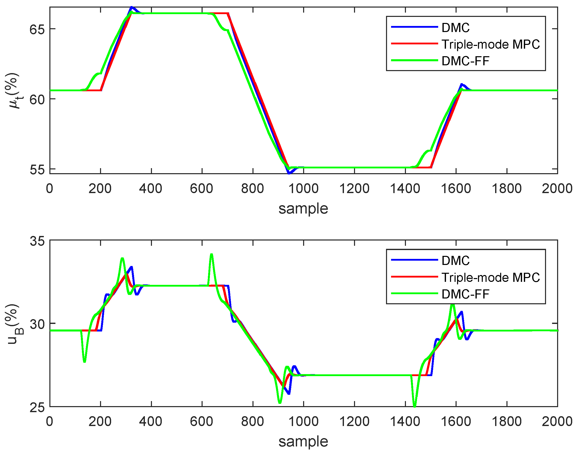
Figure 7 presents the dynamics of the controlled outputs and . The figure shows the responses obtained by the typical DMC, the triple-mode MPC and the DMC-FF algorithms. The control actions implemented by the manipulated inputs and that caused the responses in Figure 7, are shown in Figure 8.
It can be observed the output power governed by triple-mode MPC can track the load demand more quickly while maintaining steam pressure at the constant value. In contrast, the DMC-FF algorithm uses too much future target information and responses to the load demand far in advance, which leads to large oscillations in the main steam pressure. The main steam pressure controlled by the typical DMC algorithm also oscillates a lot when the load demand changes. In this case, the typical DMC algorithm even outperforms the DMC-FF algorithm due to the improper selection of future target horizon in the DMC-FF algorithm.
Table 3 reports the square errors between the output response and the desired setpoint value. In contrast, the proposed triple-mode MPC is expressed explicitly in terms of future information feedforward, and is hence expected to yield improved results for tracking performance.
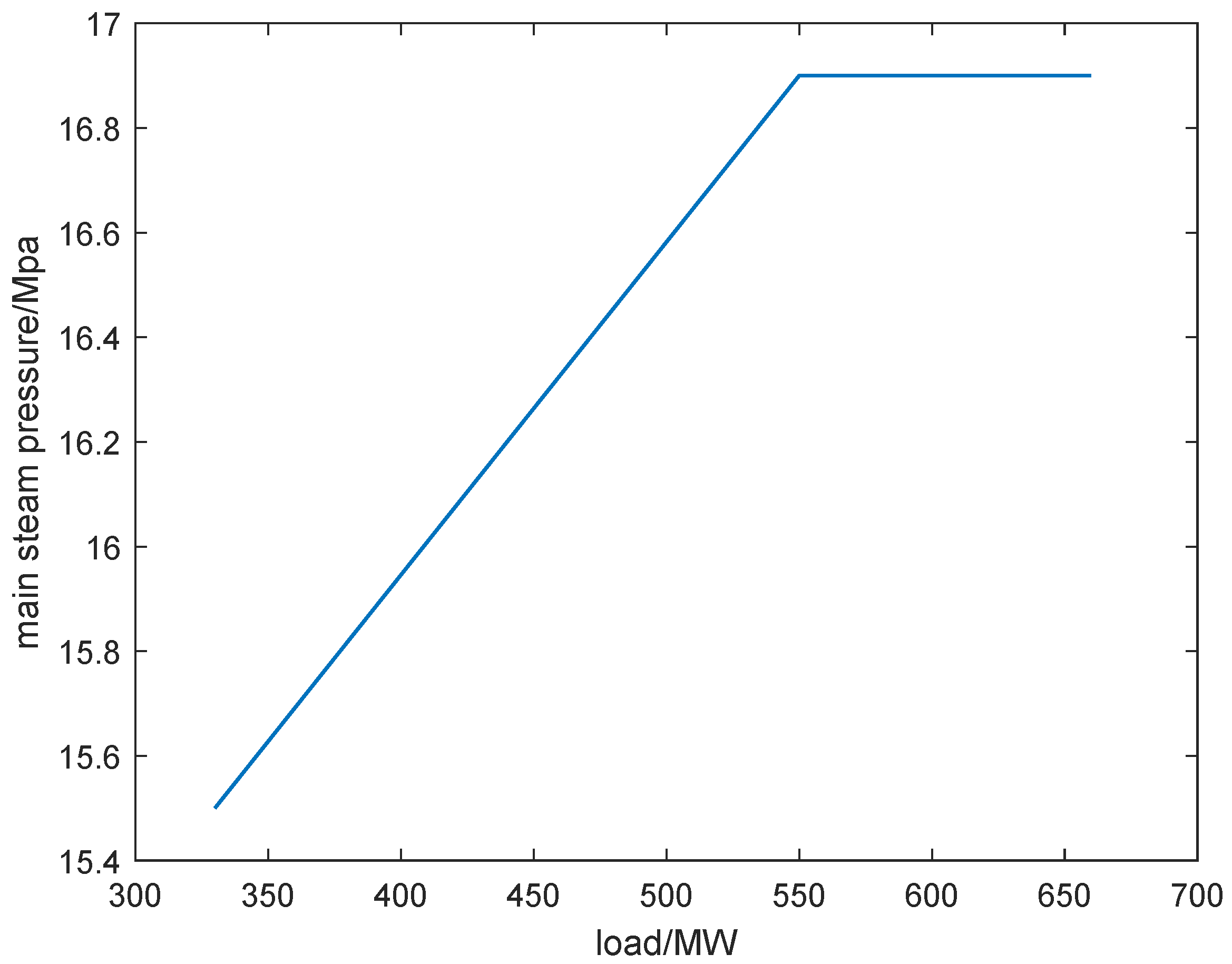
4.2.2. Sliding Pressure Operation
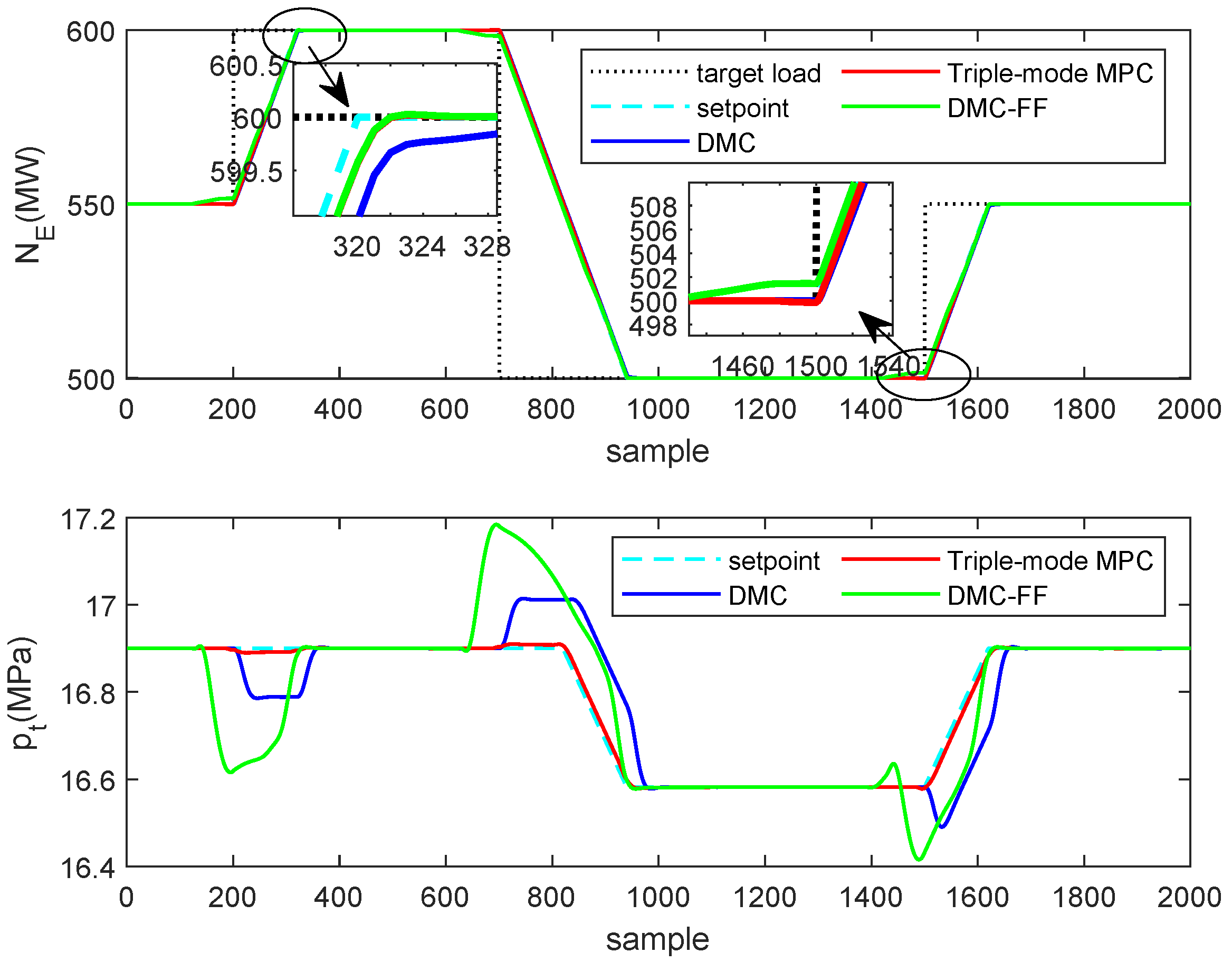
We then proceed with the running of the unit concerning sliding pressure operation, and the optimal operating curve is plotted in Figure 9. The main steam pressure increases in line with the increase of the load when the load is less than 550 MW, and maintains constant when the load exceeds 550 MW. The load demands used for tracking are the same as before.
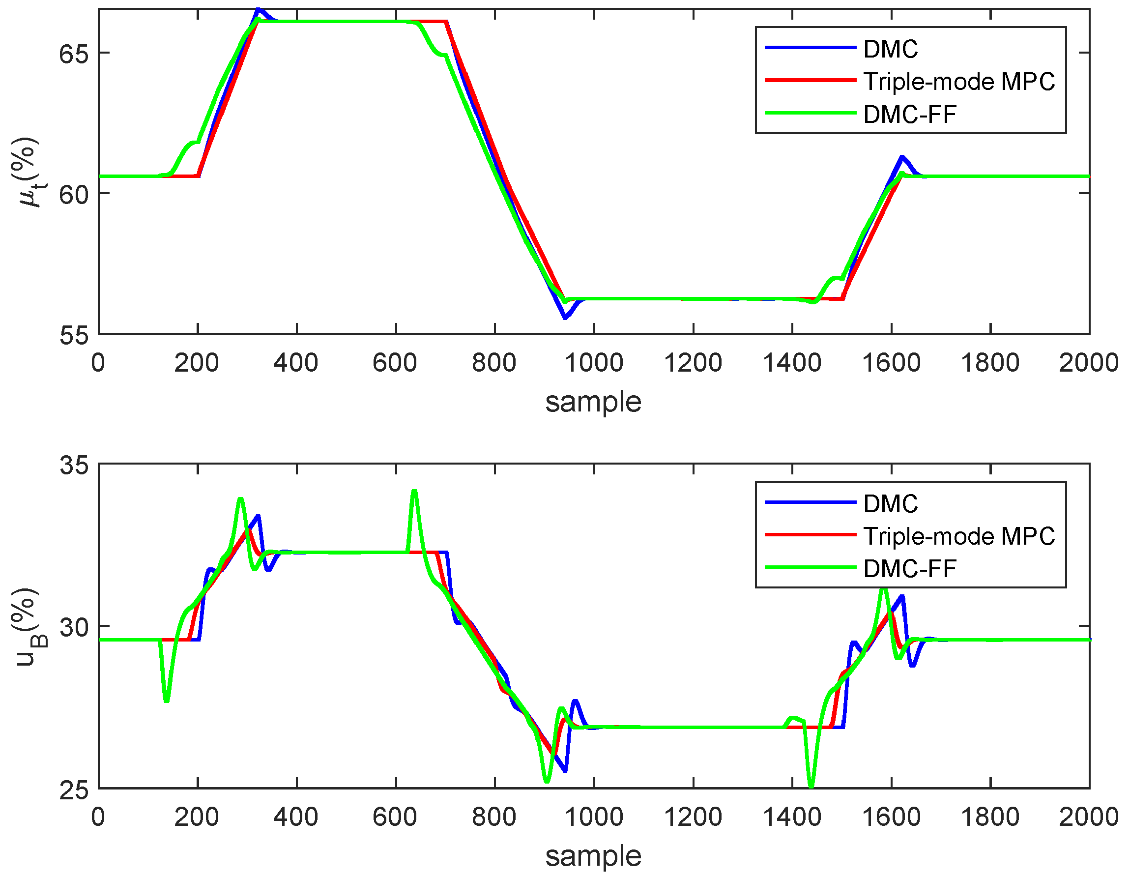
Figure 10 presents the dynamics of the controlled outputs and . The figure shows the responses obtained by the typical DMC, the proposed triple-mode MPC and the DMC-FF algorithms. The control actions implemented by the manipulated inputs and that caused the responses in Figure 10, are shown in Figure 11.
Analyzing the results in the first panel of Figure 10, one can notice that for the trajectory of the controlled output under the proposed triple-mode MPC algorithm is closer to the desired trajectory than which under the typical DMC algorithm. In addition, the trajectory governed by the DMC-FF algorithm can also respond to the load demand more quickly than the typical DMC algorithm. (The curves of triple-mode MPC and DMC-FF almost overlap in the left magnified figure) However, the DMC-FF algorithm responses to the load demand far too early, which leads to the loss of tracking performace as we can see in the right magnified figure.
On the other hand, as shown in the second panel of Figure 10, when the setpoint of the main steam pressure changes with the load demand, the accuracy of tracking deteriorates a lot under either the typical DMC or the DMC-FF algorithms. In contrast, using the triple-mode MPC can drive the main steam pressure to track its setpoint without too much performance loss.
A quantitative comparison of square errors for the whole simulation is also shown in Table 4. In the table, the power output and pressure errors of the triple-mode MPC algorithm are dramatically reduced compared to those of the typical DMC and the DMC-FF algorithms.
Remark 1.
In many practical processes such as power plants [23], wind tunnels [24], there exists future target information that can be used in feedforward design. When the MPC algorithm is applied to real systems, the closed-loop performance is related to the accuracy of the model and the future target information. If the model is consistent with the plant, and the future target information is correct, the control performance obtained is as good as which obtained in the case study.
5. Conclusions
In this work, we propose a triple-mode model predictive control algorithm using future target information. In order to explicitly take into account the future target information in the MPC optimization, the proposed triple-mode control law includes the future target information feedforward term, and the future trajectory horizon can be optimized off-line to design the feedforward. Furthermore, the extra degrees of freedom are added to append the control law such that the constraints can be met when the MPC is running. Experimental results on the shell fundamental control problem, and the coordinated control problem in the power plant demonstrate that, by incorporating future target information feedforward explicitly and using an optimal future target horizon, the proposed triple-mode MPC algorithm could better hedge against the future target information, mitigate the sluggish response, and improve the tracking performance.
Author Contributions
Methodology, Z.X. and J.Z.; Writing—original draft, M.C.; Writing—review and editing, Z.X. and J.Z.; Perform the simulations, M.C.; Analysis of results, M.C., Z.X. and J.Z. All authors have read and agreed to the published version of the manuscript.
Funding
This research was funded by National Key Research and Development Program (No. 2017YFA0700300, No. 2017YFB0603703), NSFC-Zhejiang Joint Fund for the Integration of Industrialization and Informatization (No. U1809207).
Conflicts of Interest
The authors declare no conflict of interest.
Appendix A. Proof of Theorem 1
Proof of Theorem 1.
A deviation model is obtained by computing an error model with respect to the future targets. To do so, consider a desired future trajectory described by , and define deviation variables
that satisfy the dynamic model
The zero regulation problem applied to the system in deviation variables finds that takes to zero.
Feasibility: Assume that the state at the current sample time t is . Also assume that the optimal solution is with an optimal cost . Let be the state at the next sampling time. Consider a control sequence
with . Then it is easy to see that is a feasible solution at time due to the feasibility of the optimal solution at time t and enforced terminal constraint. Consequently, .
Convergence: Consider the feasible solution at time previously presented. Following standard steps in the stability proofs of MPC (Mayne et al. [25]), we get that
Due to the definite positiveness of the optimal cost and its nonincreasing evolution, we infer that and . Consequently, the system is steered to . □
References
- Qin, S.J.; Badgwell, T.A. A survey of industrial model predictive control technology. Control Eng. Pract. 2003, 11, 733–764. [Google Scholar] [CrossRef]
- Garcia, C.E.; Morshedi, A. Quadratic programming solution of dynamic matrix control (QDMC). Chem. Eng. Commun. 1986, 46, 73–87. [Google Scholar] [CrossRef]
- Rawlings, J.B. Tutorial overview of model predictive control. IEEE Control Syst. Mag. 2000, 20, 38–52. [Google Scholar]
- Rawlings, J.B.; Mayne, D.Q. Model Predictive Control: Theory and Design; Nob Hill Pub.: San Francisco, CA, USA, 2009. [Google Scholar]
- Maciejowski, J.M. Predictive Control: With Constraints; Pearson Education: London, UK, 2002. [Google Scholar]
- Goodwin, G.; Seron, M.M.; De Doná, J.A. Constrained Control and Estimation: An Optimisation Approach; Springer Science & Business Media: Berlin, Germany, 2006. [Google Scholar]
- Zhang, K.; Zhao, J.; Zhu, Y. MPC case study on a selective catalytic reduction in a power plant. J. Process Control 2018, 62, 1–10. [Google Scholar] [CrossRef]
- Di Carlo, J.; Wensing, P.M.; Katz, B.; Bledt, G.; Kim, S. Dynamic locomotion in the mit cheetah 3 through convex model-predictive control. In Proceedings of the 2018 IEEE/RSJ International Conference on Intelligent Robots and Systems (IROS), Madrid, Spain, 1–5 October 2018; pp. 1–9. [Google Scholar]
- Limón, D.; Alvarado, I.; Alamo, T.; Camacho, E.F. MPC for tracking piecewise constant references for constrained linear systems. Automatica 2008, 44, 2382–2387. [Google Scholar] [CrossRef]
- Clarke, D.W.; Mohtadi, C. Properties of generalized predictive control. Automatica 1989, 25, 859–875. [Google Scholar] [CrossRef]
- Middleton, R.H.; Chen, J.; Freudenberg, J.S. Tracking sensitivity and achievable performance in preview control. Automatica 2004, 40, 1297–1306. [Google Scholar] [CrossRef]
- Carrasco, D.S.; Goodwin, G.C. Feedforward model predictive control. Annu. Rev. Control 2011, 35, 199–206. [Google Scholar] [CrossRef]
- Rossiter, J.; Grinnell, B. Improving the tracking of generalized predictive control controllers. Proc. Inst. Mech. Eng. Part I J. Syst. Control Eng. 1996, 210, 169–182. [Google Scholar] [CrossRef]
- Dughman, S.; Rossiter, J. Systematic and effective embedding of feedforward of target information into MPC. Int. J. Control 2017, 1–15. [Google Scholar] [CrossRef] [Green Version]
- Valencia-Palomo, G.; Rossiter, J.; López-Estrada, F. Improving the feed-forward compensator in predictive control for setpoint tracking. ISA Trans. 2014, 53, 755–766. [Google Scholar] [CrossRef] [PubMed]
- Qin, S.J.; Badgwell, T.A. An Overview of Industrial Model Predictive Control Technology; AIChE Symposium Series; American Institute of Chemical Engineers: New York, NY, USA, 1997; Volume 93, pp. 232–256. [Google Scholar]
- Kiefer, J. Sequential minimax search for a maximum. Proc. Am. Math. Soc. 1953, 4, 502–506. [Google Scholar] [CrossRef]
- Boyd, S.; Vandenberghe, L. Convex Optimization; Cambridge University Press: Cambridge, UK, 2004. [Google Scholar]
- Prett, D.M.; Morari, M. The Shell Process Control Workshop; Elsevier: Amsterdam, The Netherlands, 2013. [Google Scholar]
- Moon, U.C.; Lee, Y.; Lee, K.Y. Practical dynamic matrix control for thermal power plant coordinated control. Control Eng. Pract. 2018, 71, 154–163. [Google Scholar] [CrossRef]
- Jizhen, L.; Liang, T.; Deliang, Z.; Xinping, L. Analysis on the Nonlinearity of Load-Pressure Characteristics of a 660MW Unit. Power Eng. 2005, 25, 533–536. [Google Scholar]
- Wood, A.J.; Wollenberg, B.F.; Sheblé, G.B. Power Generation, Operation, and Control; John Wiley & Sons: Hoboken, NJ, USA, 2013. [Google Scholar]
- Flynn, D. Thermal Power Plant Simulation and Control; Number 43; IET: London, UK, 2003. [Google Scholar]
- Green, J.; Quest, J. A short history of the European Transonic Wind Tunnel ETW. Prog. Aerosp. Sci. 2011, 47, 319–368. [Google Scholar] [CrossRef]
- Mayne, D.Q.; Rawlings, J.B.; Rao, C.V.; Scokaert, P.O. Constrained model predictive control: Stability and optimality. Automatica 2000, 36, 789–814. [Google Scholar] [CrossRef]
Figure 1.
The closed-loop output response with respect to different future trajectory horizon.

Figure 2.
The evolution of golden section search for future trajectory horizon of illustrated example by using Algorithm 1.
Figure 2.
The evolution of golden section search for future trajectory horizon of illustrated example by using Algorithm 1.

Figure 3.
Schematic diagram of “Shell” heavy oil fractionator [5]. Reproduced with permission from J.M.Maciejowski, predictive control with constraints; published by Pearson education, 2002.
Figure 3.
Schematic diagram of “Shell” heavy oil fractionator [5]. Reproduced with permission from J.M.Maciejowski, predictive control with constraints; published by Pearson education, 2002.

Figure 4.
Comparison of output response obtained by DMC, triple-mode MPC and DMC-FF. The top end point is contained in the first panel and the side end point is contained in the second panel.
Figure 4.
Comparison of output response obtained by DMC, triple-mode MPC and DMC-FF. The top end point is contained in the first panel and the side end point is contained in the second panel.

Figure 5.
Comparison of input response obtained by DMC, triple-mode MPC and DMC-FF. The top draw is contained in the first panel and the side draw is contained in the second panel.
Figure 5.
Comparison of input response obtained by DMC, triple-mode MPC and DMC-FF. The top draw is contained in the first panel and the side draw is contained in the second panel.

Figure 6.
Simplified block diagram of the coordinated control system.

Figure 7.
Comparison of output response. The output power is contained in the first panel and the main steam pressure is contained in the second panel.
Figure 7.
Comparison of output response. The output power is contained in the first panel and the main steam pressure is contained in the second panel.

Figure 8.
Comparison of input response. The turbine valve is contained in the first panel and the fuel command is contained in the second panel.
Figure 8.
Comparison of input response. The turbine valve is contained in the first panel and the fuel command is contained in the second panel.

Figure 9.
Sliding pressure operation curve of the 660 MW unit.

Figure 10.
Comparison of output response. The output power is contained in the first panel and the main steam pressure is contained in the second panel.
Figure 10.
Comparison of output response. The output power is contained in the first panel and the main steam pressure is contained in the second panel.

Figure 11.
Comparison of input response. The turbine valve is contained in the first panel and the fuel command is contained in the second panel.
Figure 11.
Comparison of input response. The turbine valve is contained in the first panel and the fuel command is contained in the second panel.


Table 1.
Closed-loop system performance with different choices of f.
| ISE | 0.8055 | 0.1797 | 0.3192 |
Table 2.
Comparison of tracking error with respect to typical DMC, the triple-mode MPC and the DMC-FF algorithms.
Table 2.
Comparison of tracking error with respect to typical DMC, the triple-mode MPC and the DMC-FF algorithms.
| DMC | Triple-Mode MPC | DMC-FF | |
|---|---|---|---|
| ISE | 6.3771 | 0.7088 | 0.9515 |
Table 3.
Comparison of square errors under constant pressure operation.
| Error of (MW) | Error of (MPa) | |
|---|---|---|
| DMC | 431.7057 | 5.6357 |
| Triple-mode MPC | 104.3930 | 0.0331 |
| DMC-FF | 877.6251 | 32.3255 |
Table 4.
Comparison of square errors under sliding pressure operation.
| Error of (MW) | Error of (MPa) | |
|---|---|---|
| DMC | 501.7570 | 10.7935 |
| Triple-mode MPC | 124.5650 | 0.1009 |
| DMC-FF | 753.2611 | 22.1475 |
© 2020 by the authors. Licensee MDPI, Basel, Switzerland. This article is an open access article distributed under the terms and conditions of the Creative Commons Attribution (CC BY) license (http://creativecommons.org/licenses/by/4.0/).
Share and Cite
MDPI and ACS Style
Chen, M.; Xu, Z.; Zhao, J. Triple-Mode Model Predictive Control Using Future Target Information. Processes 2020, 8, 54. https://0-doi-org.brum.beds.ac.uk/10.3390/pr8010054
AMA Style
Chen M, Xu Z, Zhao J. Triple-Mode Model Predictive Control Using Future Target Information. Processes. 2020; 8(1):54. https://0-doi-org.brum.beds.ac.uk/10.3390/pr8010054
Chicago/Turabian StyleChen, Minghao, Zuhua Xu, and Jun Zhao. 2020. "Triple-Mode Model Predictive Control Using Future Target Information" Processes 8, no. 1: 54. https://0-doi-org.brum.beds.ac.uk/10.3390/pr8010054
Note that from the first issue of 2016, this journal uses article numbers instead of page numbers. See further details here.