Computational Optimization of Porous Structures for Electrochemical Processes
by
 , ,
, ,
Nicole Vorhauer-Huget
1,*, 
Haashir Altaf
1,2,
Robert Dürr
2,
Evangelos Tsotsas
1 and
Tanja Vidaković-Koch
2 1
Institute of Process Engineering, Otto von Guericke University Magdeburg, 39106 Magdeburg, Germany
2
Max-Planck-Institute for Dynamics of Complex Technical Systems Magdeburg, 39106 Magdeburg, Germany
*
Author to whom correspondence should be addressed.
Processes 2020, 8(10), 1205; https://0-doi-org.brum.beds.ac.uk/10.3390/pr8101205
Submission received: 10 July 2020
/
Revised: 18 September 2020
/
Accepted: 21 September 2020
/
Published: 23 September 2020
(This article belongs to the Special Issue Redesign Processes in the Age of the Fourth Industrial Revolution)
Abstract
:Porous structures are naturally involved in electrochemical processes. The specific architectures of the available porous materials, as well as their physical properties, crucially affect their applications, e.g., their use in fuel cells, batteries, or electrolysers. A key point is the correlation of transport properties (mass, heat, and charges) in the spatially—and in certain cases also temporally—distributed pore structure. In this paper, we use mathematical modeling to investigate the impact of the pore structure on the distribution of wetting and non-wetting phases in porous transport layers used in water electrolysis. We present and discuss the potential of pore network models and an upscaling strategy for the simulation of the saturation of the pore space with liquid and gas, as well as the computation of the relative permeabilities and oxygen dissolution and diffusion. It is studied how a change of structure, i.e., the spatial grading of the pore size distribution and porosity, change the transport properties. Several situations are investigated, including a vertical gradient ranging from small to large pore sizes and vice versa, as well as a dual-porosity network. The simulation results indicate that the specific porous structure has a significant impact on the spatial distribution of species and their respective relative permeabilities. In more detail, it is found that the continuous increase of pore sizes from the catalyst layer side towards the water inlet interface yields the best transport properties among the investigated pore networks. This outcome could be useful for the development of grading strategies, specifically for material optimization for improved transport kinetics in water electrolyser applications and for electrochemical processes in general.
1. Introduction
The control of process efficiency is in most cases based on the integral measurement of relevant parameters, such as the temperature, pressure, overall mass, concentration, and current density. Spatially and temporally resolved data are not available in most situations, either because of a lack of advanced equipment with high spatial and temporal resolution or because of data inaccessibility in the process. To achieve the required data accessibility in order to gain in situ information, it is often necessary to adjust the process for use with model experiments, which can result in the process deviating from reality. Furthermore, in most cases, having high spatial resolution compromises the temporal resolution. This especially restricts the research on structure interactions of porous media with overall process behavior. Examples include the application of electrodes in batteries, fuel cells, and water electrolysis [1,2,3,4,5]. Electrodes are composed of catalyst layers, gas diffusion or porous transport layers, as well as ion exchange membranes. Independent of the application, the involved porous structures are usually characterized by the ratio of the void fraction to the solid content, the average pore size and pore size distribution, the pore connectivity, the permeability, the effective diffusion coefficients, the effective thermal conductivity, and the wettability, etc. The structural material parameters are typically obtained from experimental measurements such as mercury porosimetry, BET (Brunauer-Emmett-Teller) measurement, scanning electron microscopy (SEM), microcomputed X-ray tomography (µ-CT), and even ultrasonic measurement and pulsed thermography on a larger scale [6,7,8,9,10]. From these methods, only microscopy and tomography are able to resolve the pore structure locally [11,12]. The other methods can only provide global information, such as information on the overall porosity, average pore size, and pore size distribution. In addition, transport parameters such as the relative permeability, diffusivity, thermal conductivity, and wettability are very often also determined as effective parameters that are averaged at the macro scale [13,14]. In particular situations, detailed information is required [15,16,17,18,19]. For example, transport losses in fuel cells or water electrolysis are mainly associated with the mass transfer resistances within the porous electrodes, which strongly depend on the local structure or wettability [20,21,22,23]. Various other examples are found in other research fields, such as hydrology or process engineering [24,25]. In many cases, several different substances are transported through the porous medium at the same time, and very often two-phase flow is a major issue. Especially in these situations, the distribution of species between larger and smaller pores is very relevant. While the liquid (wetting phase) and gas (non-wetting phase) are rather stagnant inside the smaller pores, pathways can develop through interconnected larger pores (Figure 1). Again, independent of the application, it is of interest to clearly identify how pores of different sizes are interconnected and how the overall architecture of the porous medium can be broken down into the local pore structure.
It is possible to analyze the impact of the distributed pore space on mass (and also heat) transfer using pore-scale modeling. Pore network models have been successfully applied to simulate water invasion in GDL microstructures used in proton exchange membrane fuel cells [26] and to simulate reactive transport [25].
In pore network modeling, two major routes are usually taken. (i) In the first option, the complex problem is simplified to single capillary experiments and simulations, as well as regular lattices [27,28,29]. More recently, with the development of more precise measurement techniques and more powerful computational tools, a second option is gaining more attention [18,30,31,32,33]. (ii) In this option, the structure of the porous medium is scanned using X-ray tomography, neutron tomography, or more recently FIB-TEM (Focused Ion Beam-Transmission Electron Microscopy) or FIB-SEM (Focused Ion Beam-Scanning Electron Microscopy) [34]. The images are then prepared for use for mass transfer simulations. Route (ii) certainly has an advantage in that the processes inside the porous medium can be visualized more realistically. However, the reliability of such models always depends on assumptions concerning the application of image filters, mesh precision, and applied thresholds in the image analysis and meshing of the computational domain. In this sense, route (i) allows more accurate physical correlation between the idealized structure and invasion.
In this paper, we sketch a general route for the estimation of transport properties based on pore network models. The application of pore network models can be useful in clarifying open questions related to the transport properties of differently structured materials, which are either estimated experimentally [14,35,36] or by macroscopic modeling [37]. Some examples are the more precise correlation of the structure and transport properties, the study of the impact of liquid cluster formation, and the role of the wetting of liquid films. As a first step, we use idealized 2D and 3D regular lattices, firstly to draw an overall picture of the impact of the pore structure on the distribution of wetting and non-wetting phases during a drainage invasion process, and secondly to develop a generic upscaling strategy using the transport coefficients and morphological data from the pore network model in a macroscopic continuum model. While we have demonstrated the relevance of pore size distribution in a recent paper related to water electrolysis [38], here the focus is on the defined gradients of the pore structure. The background for this investigation involves two factors. On the one hand, porous materials applied in electrochemical processes are very often produced with spatial gradients in the pore size [39]. In a wide range of production methods, the structure development occurs rather randomly under uncontrolled conditions [40]. Secondly, the softer materials, such as felt or foam, are very often compressed inside the technical equipment, resulting in a gradient of pore sizes [41,42]. On the other hand, it is of interest to assess how controlled grading of the pore structure can influentially impact the improvement of the overall transport kinetics of porous materials. This can be useful for classical electrochemical processes [43]. It is, therefore, important to better understand the correlation between structure and transport properties.
We introduce here a general approach that might be adapted for several situations. As an example, we use invasion of a non-wetting phase (oxygen) into a pore network saturated with a wetting phase (water) under hydrophilic conditions, as found in water electrolysis [44], and discuss the impact of the pore structure on the specific permeabilities of the partially saturated pore network. The effective parameters are applied in a continuous model to show the dynamic spatial distribution of oxygen inside the porous transport layer (PTL).
The paper is organized as follows. At first, the pore network modeling based on regular pore and throat lattices is briefly recalled in Section 2, with a focus on displacement processes occurring in the PTL during water electrolysis. In Section 3, the simulation results of the invasion of the non-wetting phase in graded pore networks are presented and discussed. They are further exploited for parameterization of a 1D macroscopic continuum model in Section 4. For this purpose, the morphological parameters obtained from the 2D pore network simulations in Section 3 will be merged into a 1D property coordinate.
2. Materials and Methods
2.1. Pore Network Model
The pore network model used in this study was developed in [45] and validated by comparison with reference experiments from the literature in [38]. The model is comprised of two tools: (i) the structure computation tool and (ii) the invasion simulation tool. At first, the structure is described extensively to give a detailed overview of the studied gradients. The invasion part is shortly summarized below—more details are given in [38,45].
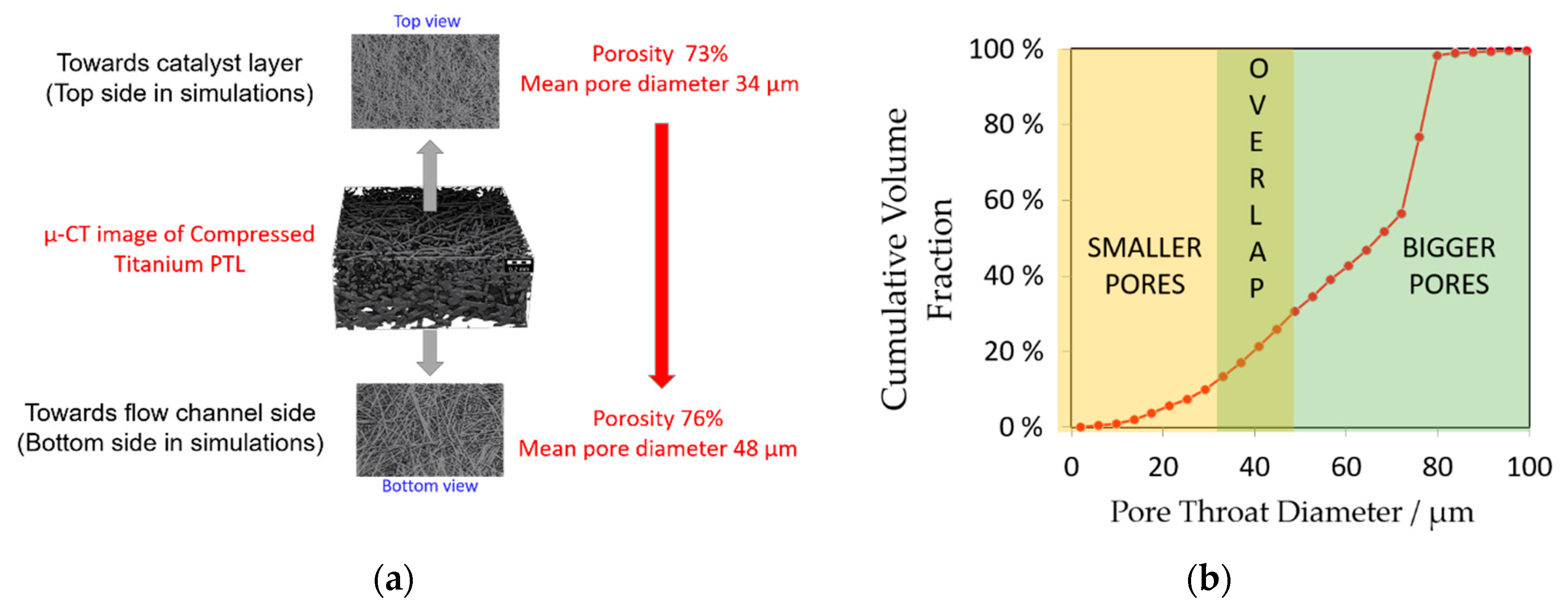
Figure 2 illustrates a very frequent example of electrochemical applications. It shows compressed titanium felt with a graded pore structure, as used in water electrolysis (Figure 2a). The mean pore sizes and porosities of the titanium felt were estimated using GeoDict (Math2Market GmbH, Kaiserslautern, Germany) (Figure 2b). As can be seen, the pore structure differs between the top and the bottom sides. More clearly, the pore size increases from the catalyst layer (applied at the top side) to the water supply channel (connected to the bottom side). The variation is mainly induced by the manufacturer and is partly a result of compression of the felt (by 10–15%) during operation.
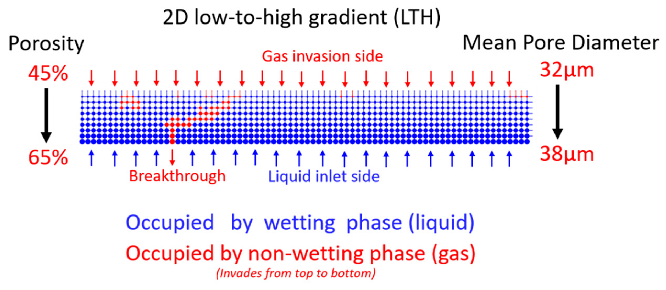
We use the example in Figure 2 as a starting point for the simulations. In more detail, we computed several pore networks with vertical gradients in pore size and porosity (note that the porosities of the regular pore network considered here are small compared to irregular porous media). In addition to the low-to-high (LTH) gradient shown in Figure 2, we also study the impact of a high-to-low (HTL) gradient. For the LTH gradient, two cases are studied. In the first case, a constant decrease in the average pore size from top to bottom is realized (Figure 3); in the second case, an abrupt change in porosity similarly as in Figure 2 is imposed on the pore structure.
2.2. Structure Tool
The mean pore and throat sizes used in the pore network simulations are based on the example shown in Figure 2. In more detail, we used cylindrical throats with diameter (or radius ) and length Lij = 50 μm = const and applied Gaussian-distributed throat sizes in the range of (Table 1). For the pores, we used a spherical geometry with the mean and standard deviation given in Table 1.
Besides the constant gradient of throat and pore sizes imposed on , with = 0.01 µm/µm for throat sizes and = 0.005 µm/µm for pore sizes (Figure 3), a dual-porosity network was realized (Figure 4 and Figure 5). Both examples result in overlapping of the throat and pore sizes of each layer, as illustrated in Figure 4 and Figure 5.
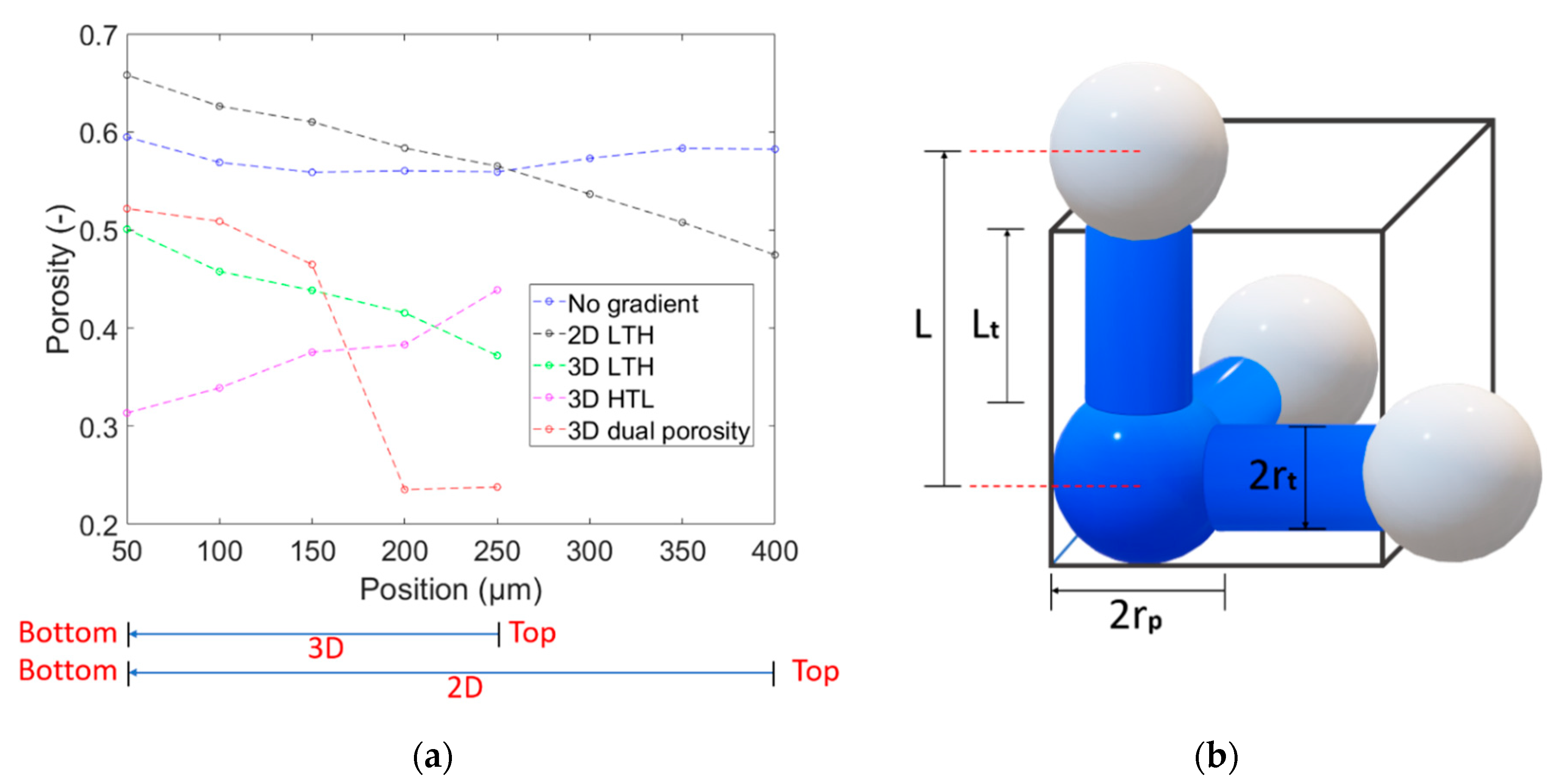
In summary, the situations studied in this work are: (1) a reference 2D network without a gradient; (2) a 2D network with a continuous LTH gradient; (3) a 3D network with a gradient identical to case 2; (4) a 3D network with the same gradient as in case 2 but in the opposite direction (i.e., HTL); (5) a 3D network with two different porosity regions (denoted as a dual-porosity pore network, similarly to Figure 2). The spatial distribution of the porosity for all cases is provided in Figure 5. As can be seen, the variation of pore sizes has a direct impact on porosity. This is explained by the constant lattice spacing, i.e., the distance between the pores, as well as the constant overall network height (width and depth in 3D).
The simulation parameters are summarized in Table 1. The pore and throat sizes, as well as the porosities, indicate the selective parameters of the investigated gradients, whereas the wetting angle ( = 60°) and temperature ( = 80 °C) are kept constant. Note that the wetting angle was chosen so as to imitate the situation of water invasion inside titanium felt. The pressure is successively increased from 1 bar to in order to enable invasion of the pore network.
2.3. Invasion Tool
The pore network simulation is based on the drainage invasion algorithm with liquid clustering presented in [38,45]. The pores and throats are initially completely filled with liquid water. Oxygen then invades from the top side by stepwise increase of the gas pressure above the critical invasion pressure thresholds of the liquid filled pores. We assume high current densities and the formation of gas fingers with plug flow of the gas phase [46]. The order of water drainage from the throats and pores is computed from the capillary pressure curve based on the Young–Laplace equation:
where is the liquid pressure, is the gas pressure, = 0.0627 kg s−2 is the surface tension of water, is the wetting angle, and is the throat radius of throat . The pore invasion is computed accordingly in competition with the throat invasion.
The invasion process is assumed as quasi-steady, capillary dominated, non-viscous flow. It is assumed that steady gas–liquid distributions are obtained at breakthrough of the gas phase to the bottom of the pore network and at disconnection of the water supply route from the bottom side to the top by further increase of the gas pressure. The model assumptions (i.e., stepwise invasion, steady-state invasion patterns) are made in accordance with experimental results reported in [46] for low capillary numbers and incompressible gas flow, as well as on the simulation results for gas permeation in [47].
Once the steady invasion profiles are obtained, gas and liquid flow rates through the partially drained pore networks are computed from the Hagen–Poiseuille equation:
Equation (2) takes into account that the transport paths for gas and liquid are hindered by isolated liquid clusters. The subscripts 1 and 2 in Equation (2) are the two pore neighbors of a throat between which the pressure gradient is considered for the computation of flow. For this, a wetting liquid and an incompressible, ideal, isothermal gas are assumed as a first step. The discrete solution of the Hagen–Poiseuille equation can be used for the computation of the relative permeabilities of gas and liquid phases at the Darcy scale, assuming laminar flow:
The value of absolute permeability is found for the same computations but with a completely saturated pore network with gas or liquid [45].
3. Results and Discussion
3.1. General Results
The 2D simulation results can only provide an orientation for the basic invasion mechanisms. In 3D, the pore connectivity is higher and different permeabilities are computed. However, the invasion profiles are very similar in 2D and 3D simulations. We, therefore, start here with the analysis of the 2D profiles before discussion of the 3D pore networks.
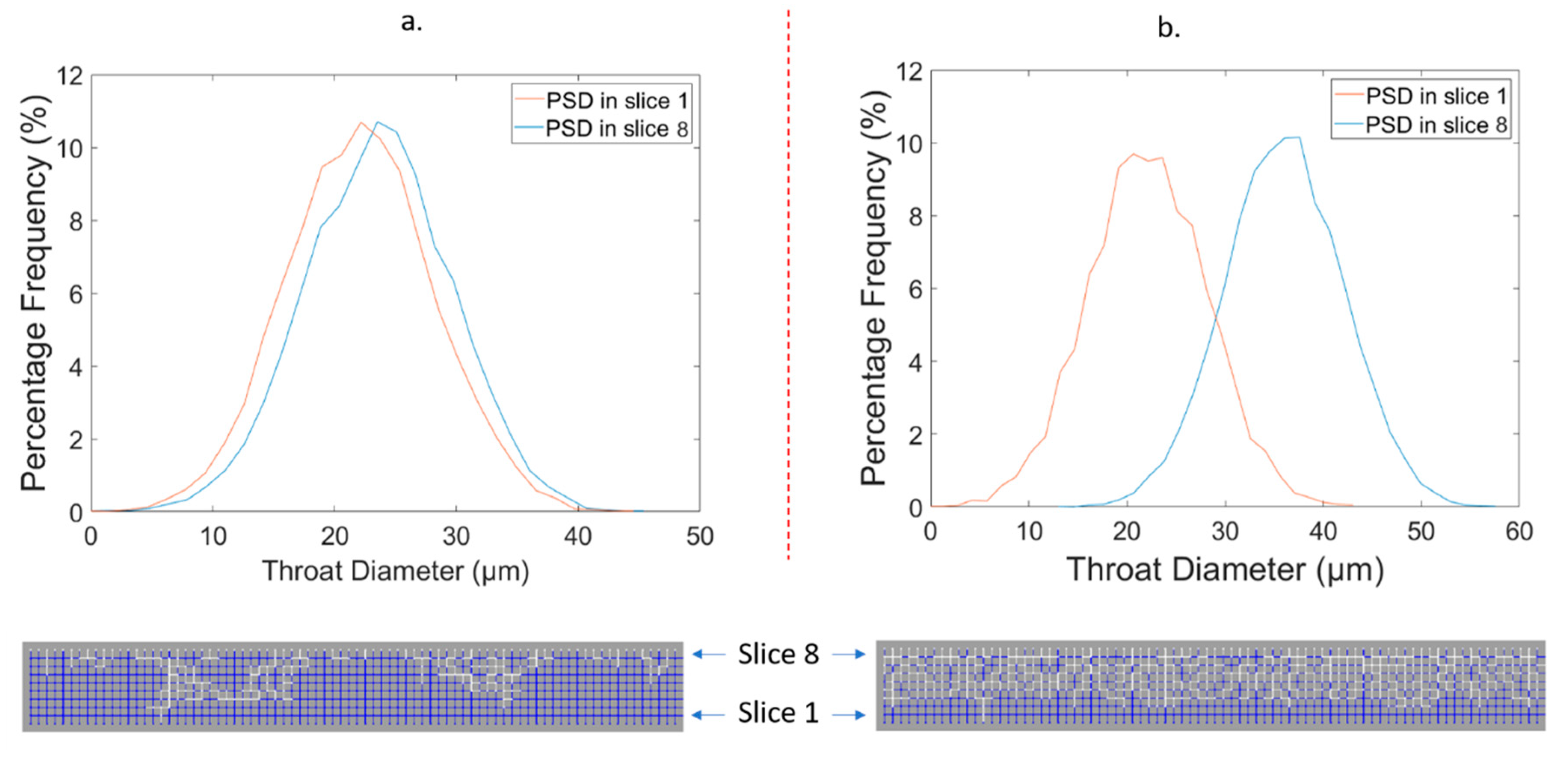
The simulated invasion patterns are very sensitive to the throat size variation in the direction of the invasion front, independent of being 2D or 3D. It has already been found that a change in the gradient can change the resulting invasion patterns. For example, gradients of = −2e−3 did result in invasion patterns similar to invasion without a gradient, whereas for = −0.02 an overlapping of throat sizes occurred and had a severe impact on the invasion patterns. This is illustrated in Figure 6 in the example of 2D simulations with HTL gradients; a similar finding was also made for 3D simulations using the same gradients. In Figure 6, the Gaussian-distributed throat sizes of selected layers of the 2D pore network are shown together with the invasion patterns. The invasion behavior changes from capillary fingering in Figure 6a to a flat front in Figure 6b. The simulations were repeated 15 times; the given invasion patterns are representative patterns. The example in Figure 6 clearly illustrates the relevance of the height of the gradient for the final saturation with gas and liquid, as well as the structure of the gas–liquid distribution.
Figure 7 summarizes the invasion profiles for 4 different gradients at breakthrough of the gas phase for both 2D and 3D simulations based on the parameters given in the previous section. In the LTH case, the larger pores are located at the bottom side. In this situation, invasion is favored towards the bottom of the network because of the lower invasion pressure thresholds that can be computed from Equation (1). Compared to the HTL simulation, the LTH is characterized by an invasion pattern such as viscous fingering [48] in both 2D and 3D simulations. Breakthrough of the gas phase occurs with a significantly lower number of invasions steps. This means that the final saturation with the gas phase at the breakthrough point is lower than compared to the HTL simulation, where the larger voids are located at the top side. In contrast to LTH, in HTL the top side is favorably invaded. Thus, in the case of HTL, the invasion results in the formation of a gas–liquid distribution, similarly as for stable displacement with a flat invasion front [48]. This is again observed in 2D and 3D simulations. However, the stabilization is more significant in 2D due to the lower pore connectivity.
3.2. Drainage Simulation
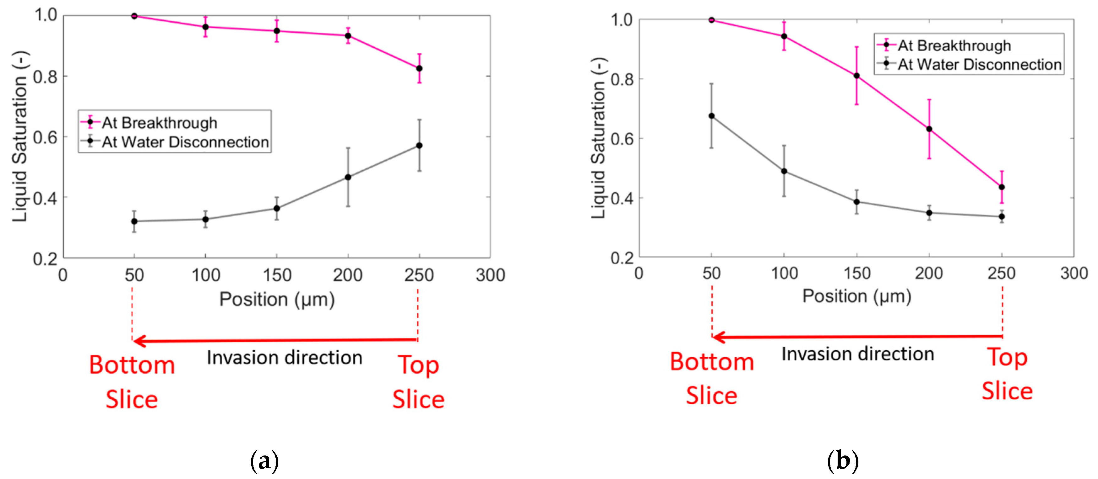
In order to obtain further insights into the impact of the gradient on the final distributions of gas and liquid and the resulting transport properties, a structure without a gradient is compared to a structure with an LTH gradient to show the effect of varying porosity. Besides the phase distributions in Figure 8, the relative gas and liquid permeabilities and saturation profiles are compared in Figure 9 and Figure 10.
The striking differences between the two simulations are the final saturations with liquid and gas phases at breakthrough, as well as the invasion behavior after breakthrough, if it is assumed that the gas phase can be forced to further invade the porous structure by increasing the gas pressure, e.g., provoked by the very low gas permeability in the studied case of laminar, incompressible gas flow (Figure 10) or based on diffusion resistances [49]. The pore network simulations indicate that the gas saturation at the top side can be reduced from around 50% to around 30% by application of a pore size gradient (Figure 9).
In the pore network without a gradient, the final liquid distribution is almost uniform across the height of the network (Figure 9; the low saturation at the bottom is explained by invasion rules and determination of liquid cluster labels [45]). In contrast, in the LTH pore network, a distinct watershed evolves in the center of the pore network, separating the gas and liquid phases. This is explained by the throat size distribution and the favorable invasion of larger throats in hydrophilic drainage.
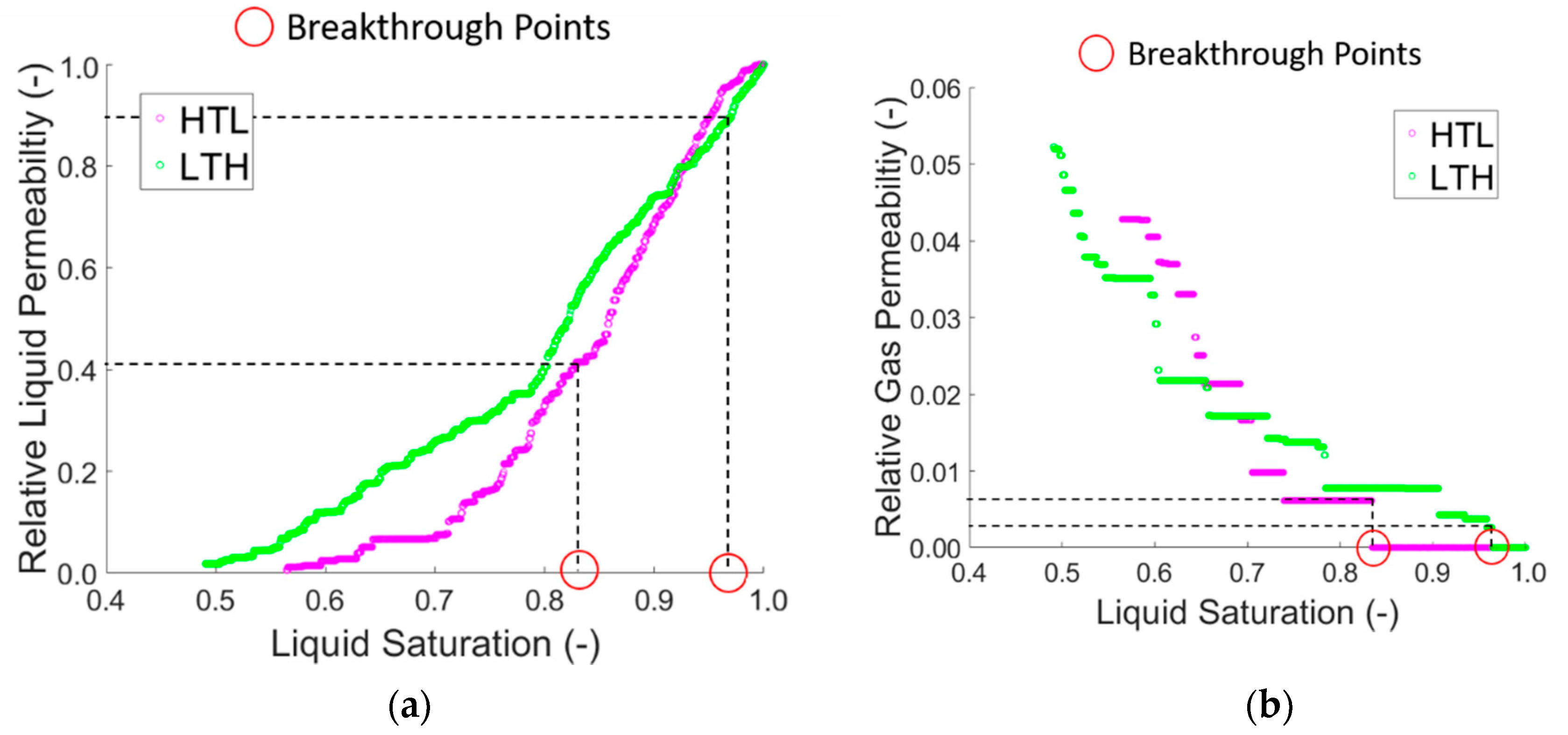
The overall liquid saturation at breakthrough is 83% inside the pore network without a gradient and 93% in the LTH network, based on the averages from 15 simulations. The final saturation with liquid is on average 35% in the pore network without a gradient and 41% in the LTH network. Thus, more liquid is contained inside the pore network with the gradient. A similar finding is reported in [46] for the application of a microporous layer. Figure 8a,c and Figure 9 reveal that the LTH gradient is very favorable for viscous fingering. As a consequence, the liquid phase has higher connectivity and less isolated liquid clusters evolve in the simulation with LTH. As shown in Figure 10, the higher liquid connectivity results in an overall higher relative liquid permeability in the pore network with the gradient (between = 0.8 and = 0.5). The absolute permeabilities computed for the empty networks are = 1.65 × 10⁻¹² m2 (network without gradient) and = 1.04 × 10⁻¹² m2 (LTH). In [50], similar absolute permeabilities in the range of 10−12 m2 to 10−10 m2 are reported for non-graded, fiber-based Ti PTLs. In detail, for pore sizes in the range of 32.4 ± 0.6 µm and porosity of 75%, the computed permeability of the non-graded structure is around 17–20 × 10−12 m2 in [50].
The two counter-current effects of liquid and gas transport induce an optimization problem in the structure in order to satisfy the optimal transport properties for both phases. From Figure 10, it can be concluded that the optimum gas–liquid configuration to obtain high liquid permeability is between the breakthrough point and S = 0.5 in case of the LTH gradient. In this range the computed gas permeability is also comparably high for the LTH gradient. This is explained by the saturation profiles, as discussed above.
Whether this issue depends on the gradient only or also on the dimension of the pore network (and thus pore connectivity) will be analyzed further using the 3D simulation results in the next section.
3.3. Drainage Simulation
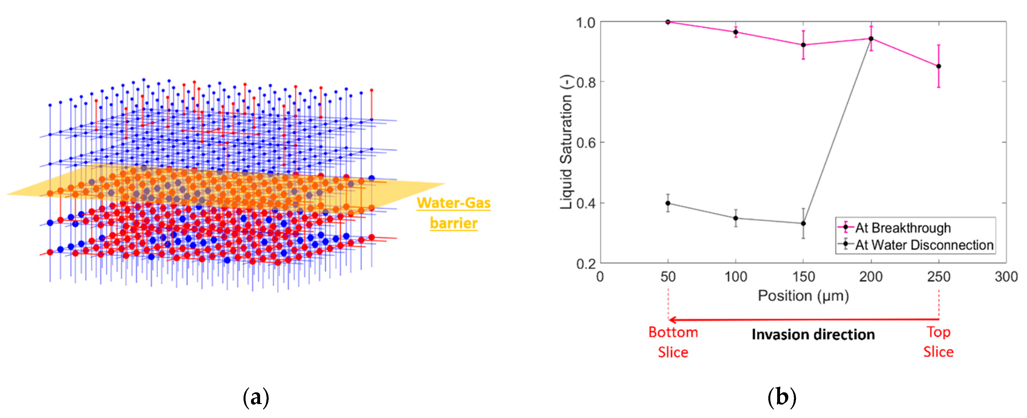
The simulation results obtained from 3D pore networks are very similar to the 2D simulation results. As shown in Figure 11 for LTH and HTL gradients, higher overall gas saturations are obtained for the HTL gradient at breakthrough, whereas in case of the LTH gradient distinct gas fingers penetrate the pore network from top to bottom. When the gas pressure is further increased after breakthrough of the gas phase, a water–gas barrier is formed in the 3D pore networks.
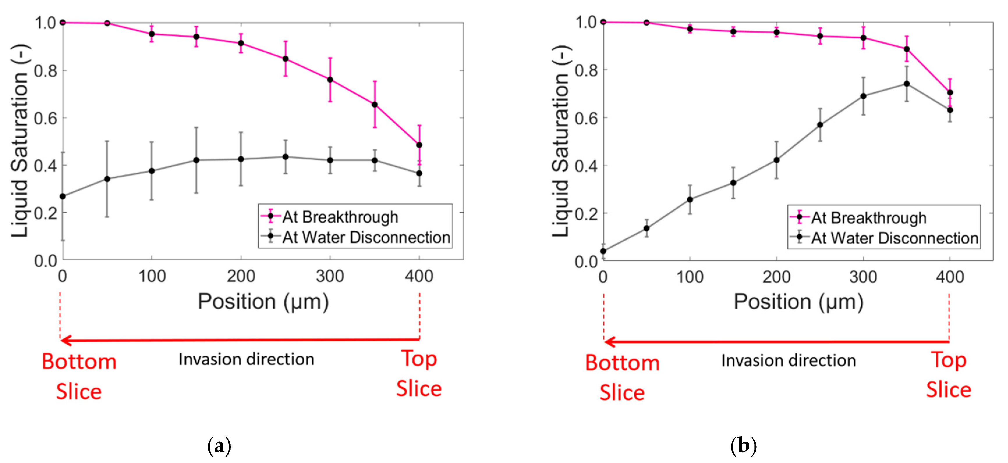
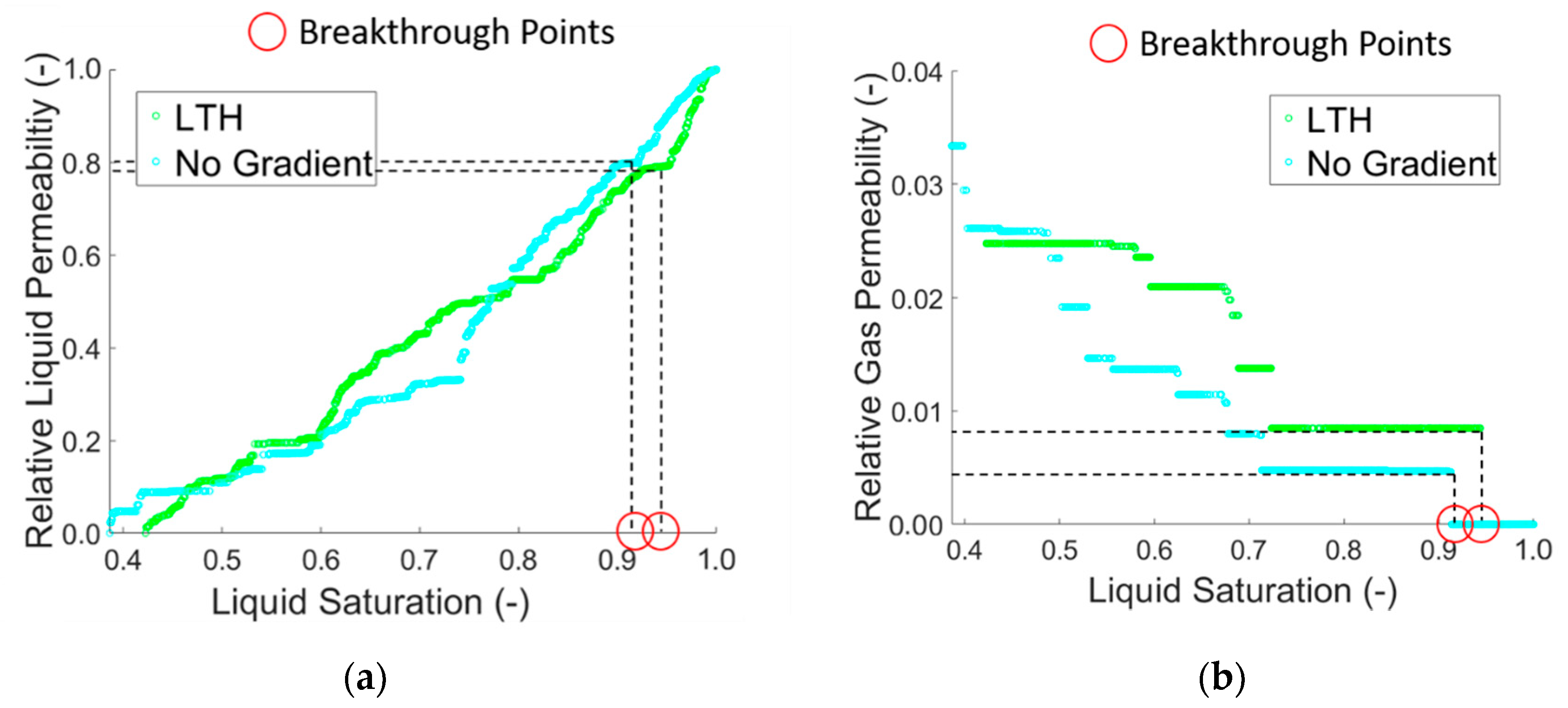
Repetition of the simulations reveals the significance of the invasion behavior. The results are summarized in Figure 12. As can be seen, the liquid saturation at breakthrough of the gas phase is almost uniform in the LTH case (Figure 12a). The highest gas saturation is at the top side, which is around 20%. This is much lower than in the 2D case, where it is around 50%. Even when the simulation is continued to further invade the pore network until disruption of the water connectivity between the top and bottom (denoted as water disconnection), the gas saturation at the top side remains low (at around 40%), while gas invasion occurs mainly at the bottom side (where the liquid saturation is lower). The behavior is opposed in the case of the HTL, where the top side always has a higher gas saturation (and lower liquid saturation, Figure 12b) than the bottom side, where the pores and throats are smaller and the resulting invasion pressures are higher. However, interestingly, the LTH and HTL invasion profiles are not perfectly inversed. Instead, significant differences occur, especially when regarding the breakthrough point, while after breakthrough the saturation profiles tend to become almost opposed (black lines in Figure 12). As shown in Figure 13 for the example of the pore–throat configuration, this strongly affects the permeabilities of the two pore networks. Overall higher relative liquid permeabilities are also found in the LTH network after breakthrough. At the same time, the relative gas permeability is also comparably higher at higher liquid saturation levels. Note that the computed gas permeabilities are generally at a low level due to the assumptions of incompressible ideal gas and slow, laminar flow. Higher values are expected for higher overall gas pressures. In summary, this indicates that the LTH pore network generally has better transport properties than the HTL network.
In Figure 14 and Figure 15, the invasion of a dual-porosity pore network is studied, with similar structure as the titanium felt in Figure 2. Figure 14a reveals distinct gas fingers form inside the low-porosity region, whereas more pore invasions occur inside the high-porosity region than in the LTH case studied above. This observation is similar to the experimental results with microporous layers in [46].
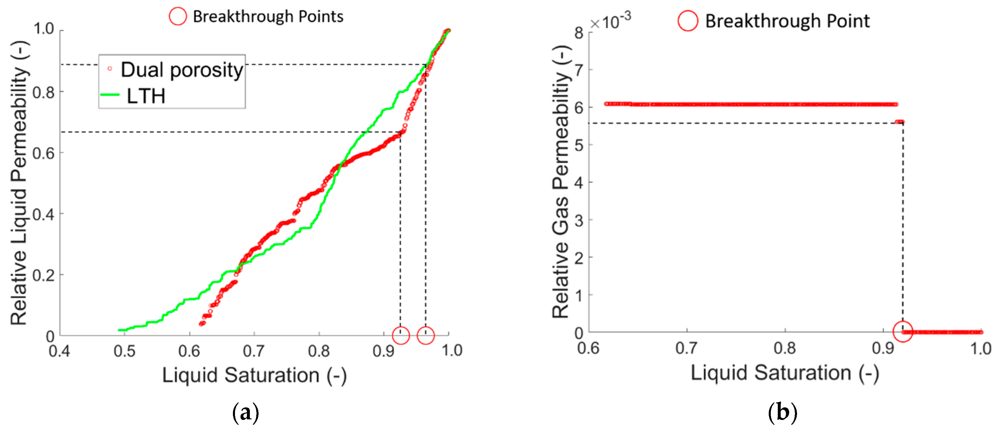
The liquid saturation inside the top layer is almost similar to the LTH gradient (Figure 12a and Figure 14b). However, in the high-porosity region, significantly more oxygen is contained when the water disconnection is regarded. This results in a higher overall gas saturation and the formation of more isolated single-liquid clusters at breakthrough and at water disconnection. As can be found in Figure 15, the liquid permeabilities of the dual-porosity network are lower than in the LTH situation. The gas permeabilities are significantly lower and remain at a constant low level because the low-porosity region is not further invaded, even if the gas pressure is increased after breakthrough.
If one deduced a grading strategy from this comparison, a pore network with an LTH gradient would be recommended over a dual-porosity pore network if low gas saturations and higher liquid permeabilities were realized. Further studies in this direction incorporating simulations of the pore structure obtained from µ-CT measurements and artificial irregular pore networks with different pore size gradients are already in progress and can be used as a base for the development of a grading strategy in the future. Validation of the outcomes using Ti–felt PTLs could be based on X-ray synchrotron imaging or neutron imaging [49,50,51], as well as on experimental data, such as from impedance spectroscopy [52,53,54]. Apart from the optimization of mass transfer properties, the change of the ohmic resistances for charge transfer must also be considered to achieve the optimal structural design [35]. Experimental studies in the literature indicate that the realization of the connectivity of the PTL with the catalyst layer and the degradation of material properties play major roles in performance enhancement [35,49,55], while other studies reveal the impacts of temperature and pressure [47].
3.4. Upscaling to Continuum Model
For the formulation and parameterization of macroscopic continuum models, such as those used to simulate fuel cells or water electrolysis on a larger scale, experimental data is usually required. Here, we would like to discuss how pore network modeling can alternatively be applied to parameterize macroscopic models. In the following, the diffusive mass transfer though the porous medium shall be regarded. This can generally be described through the correlation of the driving force, which can be a pressure gradient over distance , multiplied by a transport coefficient that is related to a resistance factor :
The resistance factor basically indicates how much of the mass transfer through a porous medium is reduced compared to diffusion across a free surface with an identical cross-section. This depends on the porosity of the porous medium:
as well as on the tortuosity , which can in the simplest form be given as the ratio of the length of a straight pore with an equivalent diameter and the same transport resistance as the porous medium, divided by the thickness of the porous medium :
Or by the ratio of the geodesic length to the Euclidian length [56]. By definition, and . In more advanced approaches, tortuosity is computed as a function of porosity, i.e., . One example is the Bruggeman relationship [57], where:
with Bruggeman exponent . However, the complex dependency of the tortuosity on the pore structure (i.e., the pore size distribution, pore length, and connectivity) makes it almost impossible to identify correctly in most situations. Thus, in most cases remains a fitting parameter. In the cases studied here, = 1, as in the pore networks with regular lattices [57]. This means that the resistance factor
becomes simply
Although more complex situations (with 1) might be studied using pore networks based on structure estimations from microscopy or tomography scans, in a first step our focus here is on porosity gradients.
In a homogeneous porous medium with equally distributed void space across the thickness, can be constant. In such situations, the effective mass flow rate could be related to the mass flow rate through the empty box as:
In a regular pore network with = 1, Equation (10) reads as:
However, in the situations studied in this paper, the porosity varies across the material. Ergo, the transport resistance also varies with height. As a consequence, as an alternative route we describe here the possibility to use the results from pore network modeling for the simulation of mass transfer through a porous medium with a pore size gradient instead of experimental estimation of spatially distributed parameters. As an example, we will discuss here the transport of dissolved oxygen in water through a partially liquid-saturated pore network. In a first step, we consider the 2D regular pore networks with the LTH gradient described above. In these networks, = 1, and thus is defined from Equation (9). The parameter of interest here is, thus, the spatially distributed porosity . In addition, in the partially saturated pore network, the ratio of the liquid phase also has to be taken into account, as the diffusion of oxygen can only occur through the interconnected water clusters. Both parameters, i.e., the spatially distributed porosity (Figure 5a) and liquid saturation (Figure 9a), were calculated for each slice of the corresponding pore networks and used in the macroscopic model, as discussed in the following section.
3.5. Macroscopic Continuum Model
As already mentioned before, we consider here the spatial and temporal distribution of the concentrations of dissolved species in the liquid phase within the partially saturated pore network. In the case of water electrolysis, the transport of dissolved oxygen through the connected water clusters is of interest. Oxygen is produced inside the catalyst layer on top of the porous transport layer (not regarded in the simulations) and then invades the PTL in the form of gas fingers. Depending on the absorption coefficient for oxygen in water at the given temperature and pressure, part of the oxygen is dissolved inside the liquid phase. The dissolved oxygen is then transported along the concentration gradient, i.e., counter-currently to the water, by diffusion. The transport direction is, thus, from top to bottom (i.e., against the direction of the z-axis).
In order to simulate oxygen diffusion inside the liquid phase, a lumped one-dimensional macroscopic model is used. The model averages transport coefficients over the cross-section of the network and describes gradients along the z-axis (thickness) of the network. In general, the concentration of a species in the liquid phase at a specific point in the network z and at time point t is given as . The dynamics of this concentration can be characterized by the following partial differential equation
Therein, denotes the fraction of the liquid phase in the network, which can be computed from the porosity and liquid saturation at each position :
which were condensed from the results of the 2D pore network simulation with the LTH pore size gradient at gas breakthrough, as presented in the previous section. Furthermore, the convective velocity of the liquid was obtained from mass conservation of the liquid flow through the network by:
with the total surface area of the network computed from the values given in Table 1. The transport of the species against the water transport direction is described by Fick’s law of diffusion, with diffusion coefficient . The source and sinks given by the absorption equilibrium of oxygen in water (which is temperature- and pressure-dependent) along the phase boundary in the vertical direction could principally be accounted for by the right-hand side term . For simplicity, we have neglected this term in this first approach. This means that oxygen is supplied only at the top side and the oxygen transfer over gas–liquid phase boundaries within the pore network is neglected.
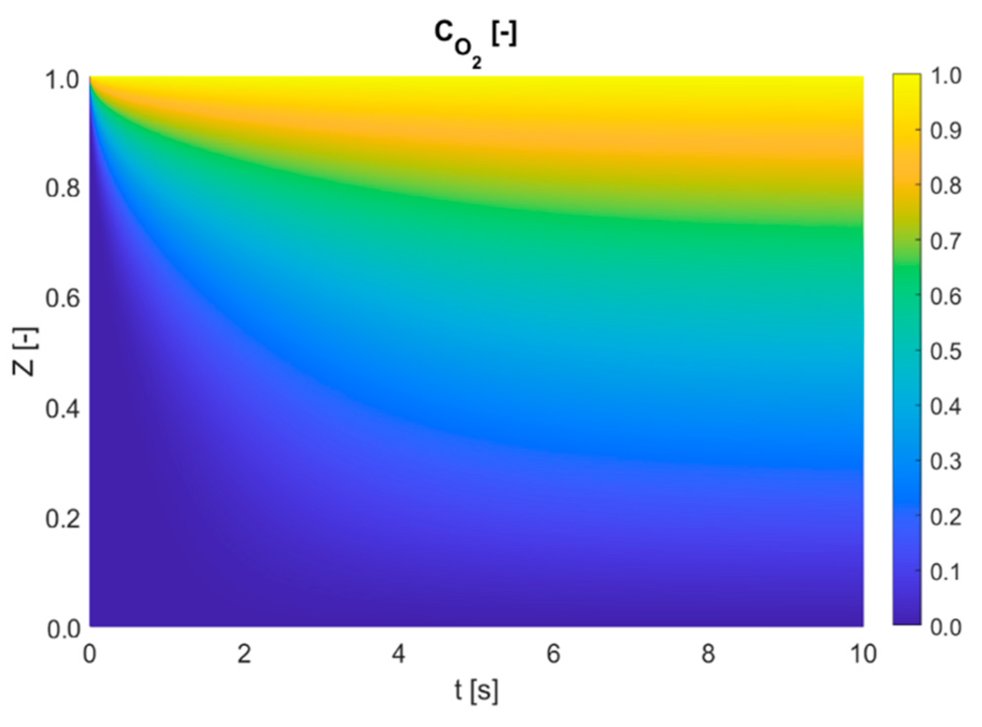
For simulation of the introduced partial differential equation, a finite volume method was applied [58,59]. The resulting set of ordinary differential equations was solved in MATLAB using ode15s [60]. The calculations are based on dimensionless variables. For this purpose, it was assumed that = 0 (initial condition) and = 1, as well as = 0 (boundary conditions). The results of the simulation are illustrated in Figure 16 for the example of the LTH gradient. As can be seen, a linear concentration profile is obtained, with a fast transition from the initial concentration profile to the steady state.
It can be deduced that the transport of dissolved oxygen in the liquid phase plays a minor role in the situation studied here, where the oxygen production rate is high enough to form gas fingers through the liquid-saturated pore network. In other words, with steady-state liquid and gas distribution, the gradient of dissolved oxygen along the height of the pore network is not high enough to transport a significant amount of additional oxygen by diffusion through the liquid phase. The high-pressure gradients over the liquid phase and the resulting high water flow rates result in significant viscous flow contributions and a low impact of oxygen diffusion. However, it is expected that oxygen diffusion could play a major role if the transport velocity of water counter-current to the oxygen diffusion direction is low.
The presented method of combined pore network simulation and macroscopic modeling is of specific interest in cases of changes of the pore network structure or changes of the liquid and gas distributions during dynamic invasion. It is a generic method that could also be applied for situations where pore and throat sizes vary over time, e.g., as a result of fouling effects or pore blocking resulting from contaminations in the liquid phase [25,61,62,63]. In such situations, a recursive procedure of alternating simulations is proposed.
4. Conclusions
In this paper, we have shown based on pore network simulations how gradients in pore sizes influence the invasion of gas into a liquid-saturated porous medium, as found in a PTL in water electrolysis. The different situations that were studied are gradients with increasing pore size in the invasion direction of the gas phase (LTH), the opposing structure (HTL), as well as a dual-porosity pore network. The simulation results were discussed for 2D and 3D pore networks. The results were compared to a pore network without a pore size gradient in a 2D simulation. It was shown that the final saturation with the gas phase decisively depends on the direction of the gradient, as well as on the design of the gradient, as the dual-porosity pore network revealed a different invasion behavior than the LTH network. Higher overall gas saturations at breakthrough of the gas phase were obtained in the case without a gradient, as well as in the pore networks with the HTL gradient, in both 2D and 3D simulations. Only when the gas pressure was increased beyond the breakthrough point did the formation of a water–gas barrier result in higher gas saturation in case of the LTH gradient. Interestingly, the obtained saturation profiles for LTH and HTL were not opposed when the breakthrough point was considered. The HTL gradient revealed a significantly lower slice saturation with liquid at the top side as compared to the results obtained for the LTH case. In the dual-porosity pore network, a low gas saturation (high liquid saturation) was observed at the low-porosity side. However, inside the high-porosity region, gas invasion resulted in the formation of more isolated liquid clusters, and thus in lower overall liquid permeability than in the LTH network, leaving some open questions for future work.
In summary, it could be demonstrated that optimization of transport properties in both phases (i.e., with high-gas and high-liquid permeabilities) is a bilateral problem, because higher gas permeabilities always result in the reduction of liquid permeability. This is especially problematic if the liquid phase is split up into a high number of isolated liquid clusters that hinder the transport of liquid and gas. This was mainly observed in the simulations without a pore size gradient, as well as in simulations with the HTL gradient and the dual-porosity pore network. In contrast, the simulation results indicate the overall better transport properties of the LTH gradient, where distinct gas fingers provide pathways for the gas phase, while at the same time maintaining high liquid permeabilities. Further systematic studies of structure optimization strategies also based on µ-CT images of different PTLs are already in progress.
Secondly, we have introduced an upscaling strategy based on combined pore network and macroscopic modeling. We showed how the distributed 2D morphological parameters porosity and liquid saturation obtained from the discrete pore network model can be lumped into a 1D macroscopic model. As an example, we discussed here the relevance of the transport of dissolved oxygen through the partially liquid-saturated pore network with the assumption of a high current density, and thus higher water flow rates. It was shown that in case of the assumption of steady-state liquid and gas distributions obtained at breakthrough of the gas phase, a constant linear oxygen profile was obtained within a few seconds. The diffusion flow rates were negligible compared to the oxygen flow through the gas fingers. However, they are expected to become much more relevant in cases of low current densities and in the transition of the transport regime from gas fingering towards bubble flow. This example reveals the possibility to couple pore network modeling and macroscopic modeling in situations where the structural effective parameters and measurement data are not available from experiments.
Symbols and Abbreviations
| Symbols | ||
| Abase | Base area | m2 |
| Normalized concentration | - | |
| Concentration | kg/m3 | |
| Diameter | µm | |
| Diffusion coefficient | m2/s | |
| Throat index | - | |
| Relative permeability | - | |
| Absolute permeability | m2 | |
| Distance between nodes | µm | |
| Length of throat | µm | |
| Mass flow rate | kg/s | |
| Capillary pressure | Pa | |
| Liquid pressure | Pa | |
| Pore radius | µm | |
| Throat radius | µm | |
| Mean radius | µm | |
| Resistance factor | kg/m3∙s | |
| Time | s | |
| Velocity | m/s | |
| Volume of pore | m3 | |
| Volume of solid | m3 | |
| Volume of throat | m3 | |
| Volume of voids | m3 | |
| Thickness of PTL | m | |
| Porosity | % | |
| Kinematic viscosity | m2/s | |
| Density of liquid | kg/m3 | |
| Contact angle | ||
| Surface tension | N/m | |
| Liquid fraction | - | |
| Tortuosity | - | |
| Abbreviations | ||
| µ-CT | Microcomputed tomography | |
| FIB | Focused ion beam | |
| HTL | High-to-low | |
| LTH | Low-to-high | |
| PSD | Pore size distribution | |
| PTL | Porous transport layer | |
| SEM | Scanning electron microscopy | |
| TEM | Transmission electron microscopy | |
Author Contributions
Conceptualization, N.V.-H.; methodology, N.V.-H.; software, N.V.-H., H.A., and R.D.; validation, H.A. and N.V.-H.; formal analysis, N.V.-H., T.V.-K., and R.D.; investigation, H.A.; resources, N.V.-H., E.T., and T.V.-K.; data curation, H.A. and R.D.; writing—original draft preparation, H.A. and N.V.-H.; writing—review and editing, N.V-H.; visualization, H.A.; supervision, N.V.-H. and T.V.-K.; project administration, N.V.-H., T.V.-K., and E.T.; funding acquisition, N.V.-H., T.V.-K., and E.T. All authors have read and agreed to the published version of the manuscript.
Funding
This research received no external funding.
Conflicts of Interest
The authors declare no conflict of interest.
References
- Grigoriev, S.A.; Millet, P.; Volobuev, S.A.; Fateev, V.N. Optimization of porous current collectors for PEM water electrolysers. Int. J. Hydrog. Energy 2009, 34, 4968–4973. [Google Scholar] [CrossRef]
- Chen, X.; Zhou, Z.; Karahan, H.E.; Shao, Q.; Wei, L.; Chen, Y. Recent Advances in Materials and Design of Electrochemically Rechargeable Zinc-Air Batteries. Small 2018, 14, e1801929. [Google Scholar] [PubMed]
- García-García, R.; García, R.E. Microstructural effects on the average properties in porous battery electrodes. J. Power Sources 2016, 309, 11–19. [Google Scholar] [CrossRef] [Green Version]
- Ye, J.; Baumgaertel, A.C.; Wang, Y.M.; Biener, J.; Biener, M.M. Structural optimization of 3D porous electrodes for high-rate performance lithium ion batteries. ACS Nano 2015, 9, 2194–2202. [Google Scholar] [PubMed]
- Xing, L.; Shi, W.; Su, H.; Xu, Q.; Das, P.K.; Mao, B.; Scott, K. Membrane electrode assemblies for PEM fuel cells: A review of functional graded design and optimization. Energy 2019, 177, 445–464. [Google Scholar] [CrossRef]
- Mayr, G.; Gresslehner, K.H.; Hendorfer, G. Non-destructive testing procedure for porosity determination in carbon fibre reinforced plastics using pulsed thermography. Quant. InfraRed Thermogr. J. 2017, 14, 263–274. [Google Scholar] [CrossRef]
- Liu, Y.; Li, X.; Chen, C.; Song, Y.; Ni, P. High throughput rapid detection for SLM manufactured elements using ultrasonic measurement. Measurement 2019, 144, 234–242. [Google Scholar] [CrossRef]
- Bardestani, R.; Patience, G.S.; Kaliaguine, S. Experimental methods in chemical engineering: Specific surface area and pore size distribution measurements—BET, BJH, and DFT. Can. J. Chem. Eng. 2019, 97, 2781–2791. [Google Scholar]
- Arbabi, F.; Kalantarian, A.; Abouatallah, R.; Wang, R.; Wallace, J.S.; Bazylak, A. Feasibility study of using microfluidic platforms for visualizing bubble flows in electrolyzer gas diffusion layers. J. Power Sources 2014, 258, 142–149. [Google Scholar] [CrossRef]
- Rigby, S.P. Structural Characterisation of Natural and Industrial Porous Materials: A Manual; Springer International Publishing: Cham, Switzerland, 2020. [Google Scholar]
- Pashminehazar, R.; Kharaghani, A.; Tsotsas, E. Three dimensional characterization of morphology and internal structure of soft material agglomerates produced in spray fluidized bed by X-ray tomography. Powder Technol. 2016, 300, 46–60. [Google Scholar] [CrossRef]
- Vilcáez, J.; Morad, S.; Shikazono, N. Pore-scale simulation of transport properties of carbonate rocks using FIB-SEM 3D microstructure: Implications for field scale solute transport simulations. J. Nat. Gas Sci. Eng. 2017, 42, 13–22. [Google Scholar] [CrossRef]
- Li, G.; Li, X.-S.; Li, C. Measurement of Permeability and Verification of Kozeny-Carman Equation Using Statistic Method. Energy Procedia 2017, 142, 4104–4109. [Google Scholar] [CrossRef]
- Suermann, M.; Takanohashi, K.; Lamibrac, A.; Schmidt, T.J.; Büchi, F.N. Influence of Operating Conditions and Material Properties on the Mass Transport Losses of Polymer Electrolyte Water Electrolysis. J. Electrochem. Soc. 2017, 164, F973. [Google Scholar] [CrossRef] [Green Version]
- Piller, M.; Casagrande, D.; Schena, G.; Santini, M. Pore-scale simulation of laminar flow through porous media. J. Phys. Conf. Ser. 2014, 501, 12010. [Google Scholar] [CrossRef]
- AlRatrout, A.; Blunt, M.J.; Bijeljic, B. Spatial Correlation of Contact Angle and Curvature in Pore-Space Images. Water Resour. Res. 2018, 54, 6133–6152. [Google Scholar] [CrossRef] [Green Version]
- Börnhorst, M.; Walzel, P.; Rahimi, A.; Kharaghani, A.; Tsotsas, E.; Nestle, N.; Besser, A.; Kleine Jäger, F.; Metzger, T. Influence of pore structure and impregnation–drying conditions on the solid distribution in porous support materials. Dry. Technol. 2016, 34, 1964–1978. [Google Scholar] [CrossRef]
- Halter, J.; Bevilacqua, N.; Zeis, R.; Schmidt, T.J.; Büchi, F.N. The impact of the catalyst layer structure on phosphoric acid migration in HT-PEFC—An operando X-ray tomographic microscopy study. J. Electroanal. Chem. 2020, 859, 113832. [Google Scholar] [CrossRef]
- Kunz, P.; Paulisch, M.; Osenberg, M.; Bischof, B.; Manke, I.; Nieken, U. Prediction of Electrolyte Distribution in Technical Gas Diffusion Electrodes: From Imaging to SPH Simulations. Transp. Porous Med. 2020, 132, 381–403. [Google Scholar] [CrossRef] [Green Version]
- Carmo, M.; Fritz, D.L.; Mergel, J.; Stolten, D. A comprehensive review on PEM water electrolysis. Int. J. Hydrogen Energy 2013, 38, 4901–4934. [Google Scholar] [CrossRef]
- Chevalier, S.; Fazeli, M.; Mack, F.; Galbiati, S.; Manke, I.; Bazylak, A.; Zeis, R. Role of the microporous layer in the redistribution of phosphoric acid in high temperature PEM fuel cell gas diffusion electrodes. Electrochim. Acta 2016, 212, 187–194. [Google Scholar] [CrossRef]
- Sinha, P.K.; Wang, C.-Y. Liquid water transport in a mixed-wet gas diffusion layer of a polymer electrolyte fuel cell. Chem. Eng. Sci. 2008, 63, 1081–1091. [Google Scholar] [CrossRef]
- Liu, T.; Lin, J.; Wu, H.; Xia, C.; Chen, C.; Zhan, Z. Tailoring the pore structure of cathode supports for improving the electrochemical performance of solid oxide fuel cells. J. Electroceram. 2018, 40, 138–143. [Google Scholar] [CrossRef]
- Dashtian, H.; Shokri, N.; Sahimi, M. Pore-network model of evaporation-induced salt precipitation in porous media: The effect of correlations and heterogeneity. Adv. Water Resour. 2018, 112, 59–71. [Google Scholar] [CrossRef] [Green Version]
- Xiong, Q.; Baychev, T.G.; Jivkov, A.P. Review of pore network modelling of porous media: Experimental characterisations, network constructions and applications to reactive transport. J. Contam. Hydrol. 2016, 192, 101–117. [Google Scholar] [CrossRef]
- Agaesse, T.; Lamibrac, A.; Büchi, F.N.; Pauchet, J.; Prat, M. Validation of pore network simulations of ex-situ water distributions in a gas diffusion layer of proton exchange membrane fuel cells with X-ray tomographic images. J. Power Sources 2016, 331, 462–474. [Google Scholar] [CrossRef] [Green Version]
- Chauvet, F.; Duru, P.; Geoffroy, S.; Prat, M. Three periods of drying of a single square capillary tube. Phys. Rev. Lett. 2009, 103, 124502. [Google Scholar] [CrossRef] [Green Version]
- Naillon, A.; Duru, P.; Marcoux, M.; Prat, M. Evaporation with sodium chloride crystallization in a capillary tube. J. Cryst. Growth 2015, 422, 52–61. [Google Scholar] [CrossRef] [Green Version]
- Vorhauer, N.; Tsotsas, E.; Prat, M. Temperature gradient induced double stabilization of the evaporation front within a drying porous medium. Phys. Rev. Fluids 2018, 3, 217. [Google Scholar] [CrossRef] [Green Version]
- Shokri, N.; Lehmann, P.; Vontobel, P.; Or, D. Drying front and water content dynamics during evaporation from sand delineated by neutron radiography. Water Resour. Res. 2008, 44, 815. [Google Scholar] [CrossRef] [Green Version]
- Blunt, M.J.; Bijeljic, B.; Dong, H.; Gharbi, O.; Iglauer, S.; Mostaghimi, P.; Paluszny, A.; Pentland, C. Pore-scale imaging and modelling. Adv. Water Resour. 2013, 51, 197–216. [Google Scholar] [CrossRef] [Green Version]
- Ceballos, L.; Prat, M.; Duru, P. Slow invasion of a nonwetting fluid from multiple inlet sources in a thin porous layer. Phys. Rev. E Stat. Nonlinear Soft Matter Phys. 2011, 84, 56311. [Google Scholar] [CrossRef] [PubMed]
- Ceballos, L.; Prat, M. Slow invasion of a fluid from multiple inlet sources in a thin porous layer: Influence of trapping and wettability. Phys. Rev. E Stat. Nonlinear Soft Matter Phys. 2013, 87, 43005. [Google Scholar] [CrossRef] [PubMed] [Green Version]
- Saif, T.; Lin, Q.; Butcher, A.R.; Bijeljic, B.; Blunt, M.J. Multi-scale multi-dimensional microstructure imaging of oil shale pyrolysis using X-ray micro-tomography, automated ultra-high resolution SEM, MAPS Mineralogy and FIB-SEM. Appl. Energy 2017, 202, 628–647. [Google Scholar] [CrossRef]
- Majasan, J.O.; Iacoviello, F.; Cho, J.I.S.; Maier, M.; Lu, X.; Neville, T.P.; Dedigama, I.; Shearing, P.R.; Brett, D.J.L. Correlative study of microstructure and performance for porous transport layers in polymer electrolyte membrane water electrolysers by X-ray computed tomography and electrochemical characterization. Int. J. Hydrog. Energy 2019, 44, 19519–19532. [Google Scholar] [CrossRef]
- Lettenmeier, P.; Kolb, S.; Sata, N.; Fallisch, A.; Zielke, L.; Thiele, S.; Gago, A.S.; Friedrich, K.A. Comprehensive investigation of novel pore-graded gas diffusion layers for high-performance and cost-effective proton exchange membrane electrolyzers. Energy Environ. Sci. 2017, 10, 2521–2533. [Google Scholar] [CrossRef] [Green Version]
- Schmidt, G.; Suermann, M.; Bensmann, B.; Hanke-Rauschenbach, R.; Neuweiler, I. Modeling Overpotentials Related to Mass Transport Through Porous Transport Layers of PEM Water Electrolysis Cells. J. Electrochem. Soc. 2020, 167, 114511. [Google Scholar] [CrossRef]
- Altaf, H.; Vorhauer, N.; Tsotsas, E.; Vidaković-Koch, T. Steady-State Water Drainage by Oxygen in Anodic Porous Transport Layer of Electrolyzers: A 2D Pore Network Study. Processes 2020, 8, 362. [Google Scholar] [CrossRef] [Green Version]
- Deiner, L.J.; Reitz, T.L. Inkjet and Aerosol Jet Printing of Electrochemical Devices for Energy Conversion and Storage. Adv. Eng. Mater. 2017, 19, 1600878. [Google Scholar] [CrossRef]
- Talukdar, K.; Delgado, S.; Lagarteira, T.; Gazdzicki, P.; Friedrich, K.A. Minimizing mass-transport loss in proton exchange membrane fuel cell by freeze-drying of cathode catalyst layers. J. Power Sources 2019, 427, 309–317. [Google Scholar] [CrossRef]
- Shrestha, P.; Ouellette, D.; Lee, J.; Ge, N.; Wong, A.K.C.; Muirhead, D.; Liu, H.; Banerjee, R.; Bazylak, A. Graded Microporous Layers for Enhanced Capillary-Driven Liquid Water Removal in Polymer Electrolyte Membrane Fuel Cells. Adv. Mater. Interfaces 2019, 6, 1901157. [Google Scholar] [CrossRef]
- Bevilacqua, N.; Eifert, L.; Banerjee, R.; Köble, K.; Faragó, T.; Zuber, M.; Bazylak, A.; Zeis, R. Visualization of electrolyte flow in vanadium redox flow batteries using synchrotron X-ray radiography and tomography—Impact of electrolyte species and electrode compression. J. Power Sources 2019, 439, 227071. [Google Scholar] [CrossRef]
- Balakrishnan, M.; Shrestha, P.; Ge, N.; Lee, C.; Fahy, K.F.; Zeis, R.; Schulz, V.P.; Hatton, B.D.; Bazylak, A. Designing Tailored Gas Diffusion Layers with Pore Size Gradients via Electrospinning for Polymer Electrolyte Membrane Fuel Cells. ACS Appl. Energy Mater. 2020, 3, 2695–2707. [Google Scholar] [CrossRef]
- Shiva Kumar, S.; Himabindu, V. Hydrogen production by PEM water electrolysis—A review. Mater. Sci. Energy Technol. 2019, 2, 442–454. [Google Scholar] [CrossRef]
- Vorhauer, N.; Altaf, H.; Tsotsas, E.; Vidakovic-Koch, T. Pore Network Simulation of Gas-Liquid Distribution in Porous Transport Layers. Processes 2019, 7, 558. [Google Scholar] [CrossRef] [Green Version]
- Lee, C.; Zhao, B.; Abouatallah, R.; Wang, R.; Bazylak, A. Compressible-Gas Invasion into Liquid-Saturated Porous Media: Application to Polymer-Electrolyte-Membrane Electrolyzers. Phys. Rev. Appl. 2019, 11, 054029. [Google Scholar] [CrossRef]
- Garcia-Navarro, J.; Schulze, M.; Friedrich, K.A. Understanding the Role of Water Flow and the Porous Transport Layer on the Performance of Proton Exchange Membrane Water Electrolyzers. ACS Sustain. Chem. Eng. 2019, 7, 1600–1610. [Google Scholar] [CrossRef]
- Lenormand, R. Liquids in porous media. J. Phys. Condens. Matter 1990, 2, SA79–SA88. [Google Scholar] [CrossRef]
- Lee, C.; Lee, J.K.; Zhao, B.; Fahy, K.F.; Bazylak, A. Transient Gas Distribution in Porous Transport Layers of Polymer Electrolyte Membrane Electrolyzers. J. Electrochem. Soc. 2020, 167, 24508. [Google Scholar] [CrossRef]
- Schuler, T.; de Bruycker, R.; Schmidt, T.J.; Büchi, F.N. Polymer Electrolyte Water Electrolysis: Correlating Porous Transport Layer Structural Properties and Performance: Part I. Tomographic Analysis of Morphology and Topology. J. Electrochem. Soc. 2019, 166, F270–F281. [Google Scholar] [CrossRef] [Green Version]
- Lee, C.; Lee, J.K.; Zhao, B.; Fahy, K.F.; LaManna, J.M.; Baltic, E.; Hussey, D.S.; Jacobson, D.L.; Schulz, V.P.; Bazylak, A. Temperature-dependent gas accumulation in polymer electrolyte membrane electrolyzer porous transport layers. J. Power Sources 2020, 446, 227312. [Google Scholar] [CrossRef]
- Siracusano, S.; Trocino, S.; Briguglio, N.; Baglio, V.; Aricò, A.S. Electrochemical Impedance Spectroscopy as a Diagnostic Tool in Polymer Electrolyte Membrane Electrolysis. Materials 2018, 11, 1368. [Google Scholar] [CrossRef] [PubMed] [Green Version]
- Bernt, M.; Siebel, A.; Gasteiger, H.A. Analysis of Voltage Losses in PEM Water Electrolyzers with Low Platinum Group Metal Loadings. J. Electrochem. Soc. 2018, 165, F305–F314. [Google Scholar] [CrossRef]
- Millet, P.; Ngameni, R.; Grigoriev, S.A.; Mbemba, N.; Brisset, F.; Ranjbari, A.; Etiévant, C. PEM water electrolyzers: From electrocatalysis to stack development. Int. J. Hydrog. Energy 2010, 35, 5043–5052. [Google Scholar] [CrossRef]
- Liu, C.; Carmo, M.; Bender, G.; Everwand, A.; Lickert, T.; Young, J.L.; Smolinka, T.; Stolten, D.; Lehnert, W. Performance enhancement of PEM electrolyzers through iridium-coated titanium porous transport layers. Electrochem. Commun. 2018, 97, 96–99. [Google Scholar] [CrossRef]
- Roque, W.L.; Costa, R.R.A. A plugin for computing the pore/grain network tortuosity of a porous medium from 2D/3D MicroCT image. Appl. Comput. Geosci. 2020, 5, 100019. [Google Scholar] [CrossRef]
- Thorat, I.V.; Stephenson, D.E.; Zacharias, N.A.; Zaghib, K.; Harb, J.N.; Wheeler, D.R. Quantifying tortuosity in porous Li-ion battery materials. J. Power Sources 2009, 188, 592–600. [Google Scholar] [CrossRef]
- LeVeque, R.J. Numerical Methods for Conservation Laws; Birkhäuser Basel: Basel, Switzerland, 1990. [Google Scholar]
- Hundsdorfer, W.; Verwer, J. Numerical Solution of Time-Dependent Advection-Diffusion-Reaction Equations; Springer: Berlin/Heidelberg, Germany, 2003. [Google Scholar]
- Shampine, L.F.; Gladwell, I.; Thompson, S. Solving ODEs with MATLAB; Cambridge University Press: Cambridge, UK, 2009. [Google Scholar]
- Griffiths, I.M.; Kumar, A.; Stewart, P.S. A combined network model for membrane fouling. J. Colloid Interface Sci. 2014, 432, 10–18. [Google Scholar] [CrossRef] [Green Version]
- Debnath, N.; Kumar, A.; Thundat, T.; Sadrzadeh, M. Investigating fouling at the pore-scale using a microfluidic membrane mimic filtration system. Sci. Rep. 2019, 9, 10587. [Google Scholar] [CrossRef] [Green Version]
- Xu, J.; Sheng, G.-P.; Luo, H.-W.; Li, W.-W.; Wang, L.-F.; Yu, H.-Q. Fouling of proton exchange membrane (PEM) deteriorates the performance of microbial fuel cell. Water Res. 2012, 46, 1817–1824. [Google Scholar] [CrossRef]
Figure 1.
Schematic illustration of the impact of the pore structure on the transport properties. Solid spaces are indicated in black and pore spaces are indicated in white and blue, depending on the saturation with wetting and non-wetting phases. The blue phase (which is the wetting phase here) finds pathways through the larger connected pores (indicated by the green arrows), whereas stagnation (orange arrows) occurs in dead ends. The small pores remain uninvaded (shown in white).

Figure 2.
(a) Compressed titanium felt (from SylaTech Germany; dfibre = 20–45 µm, thickness 1.02 mm, original porosity 80%) after application at the anode in water electrolysis. The pore sizes at the top side are smaller than throughout the rest of the material. This results in different porosities at the top and bottom sides. The images were obtained from microcomputed tomography (CT-Alpha from Procon X-Ray GmbH, Sarstedt, Germany). (b) Cumulative volume fraction of measured pore sizes. The region denoted as “smaller pores” refers to the top side of the felt and the region denoted as “larger pores” refers to the bottom side, cutting the felt in half at its horizontal axis. Both layers have an overlap of pore sizes as indicated. PTL denotes the porous transport layer.

Figure 3.
Visualization of the pore structure gradient in a 2D pore network. Here, the low-to-high (LTH) gradient is illustrated. It is shown how the structure can be occupied by gas (non-wetting) and liquid (wetting) phases simultaneously.
Figure 3.
Visualization of the pore structure gradient in a 2D pore network. Here, the low-to-high (LTH) gradient is illustrated. It is shown how the structure can be occupied by gas (non-wetting) and liquid (wetting) phases simultaneously.

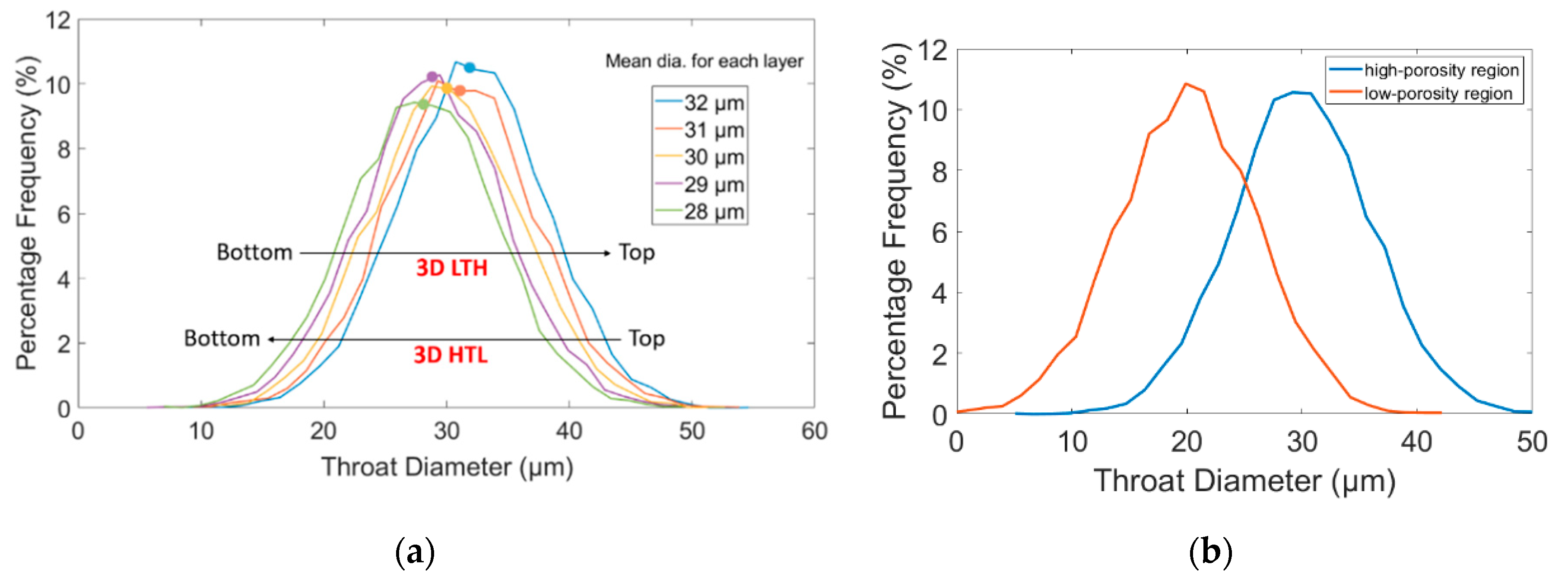
Figure 4.
Visualization of the layered pore size distributions investigated in this study: (a) 3D low-to-high (LTH) and high-to-low gradients (HTL); (b) 3D dual-porosity network (only the curves of the two regions are shown). Note that a pore network slice is comprised of one horizontal layer of throats (in vertical and horizontal direction) and one pore layer. For this reason, the data points of only 5 slices are shown in (a) for the 3D pore network.

Figure 5.
(a) Spatial variation of porosity in the 5 cases studied in this work. Only the porosity values of the slices in the center of the pore network are provided. (b) Graphical illustration of a volume element used for porosity computation. The blue cylinders and the sphere represent the throats and the pore that are accounted for the volume element, respectively. The white spheres represent the pore neighbors from the neighboring volume element. indicates the lattice spacing, is the throat length, and and are the throat radius and pore radius, respectively.

Figure 6.
Impact of the height of the gradient on invasion patterns in the example of a 2D simulation: (a) pore network with = −2e−3; (b) pore network with = −0.02. Shown are slices 1 (brown) and 8 (blue). PSD denotes pores size distribution.
Figure 6.
Impact of the height of the gradient on invasion patterns in the example of a 2D simulation: (a) pore network with = −2e−3; (b) pore network with = −0.02. Shown are slices 1 (brown) and 8 (blue). PSD denotes pores size distribution.

Figure 7.
Overview of the different invasion patterns obtained from the simulation of hydrophilic drainage in 2D and 3D pore networks with vertical gradients of pore size and porosity.
Figure 7.
Overview of the different invasion patterns obtained from the simulation of hydrophilic drainage in 2D and 3D pore networks with vertical gradients of pore size and porosity.

Figure 8.
Comparison of invasion patterns of 2D pore networks without grading and with LTH grading. The pore networks are invaded from top to bottom. This means that the top layer is connected to the oxygen source and the bottom layer is connected to the water source. The simulation results are compared at the breakthrough point and at the point when the water connectivity between the top layer and bottom layer is lost. (a) Breakthrough patterns in the pore network without gradient. (b) Network from (a) with interrupted water connectivity between the top and bottom sides. (c) Network with LTH gradient at breakthrough. (d) The same network as in (c) after water disconnection.

Figure 9.
(a) Saturation profiles for the networks in Figure 8a,b (no gradient) and (b) for Figure 8c,d (LTH gradient). The graphs were obtained from Monte Carlo simulation of 15 variations of the pore networks, with simulation parameters as summarized in Table 1.

Figure 10.
(a) Relative liquid permeability and (b) relative gas permeability of the 2D pore network simulations from Figure 8.
Figure 10.
(a) Relative liquid permeability and (b) relative gas permeability of the 2D pore network simulations from Figure 8.

Figure 11.
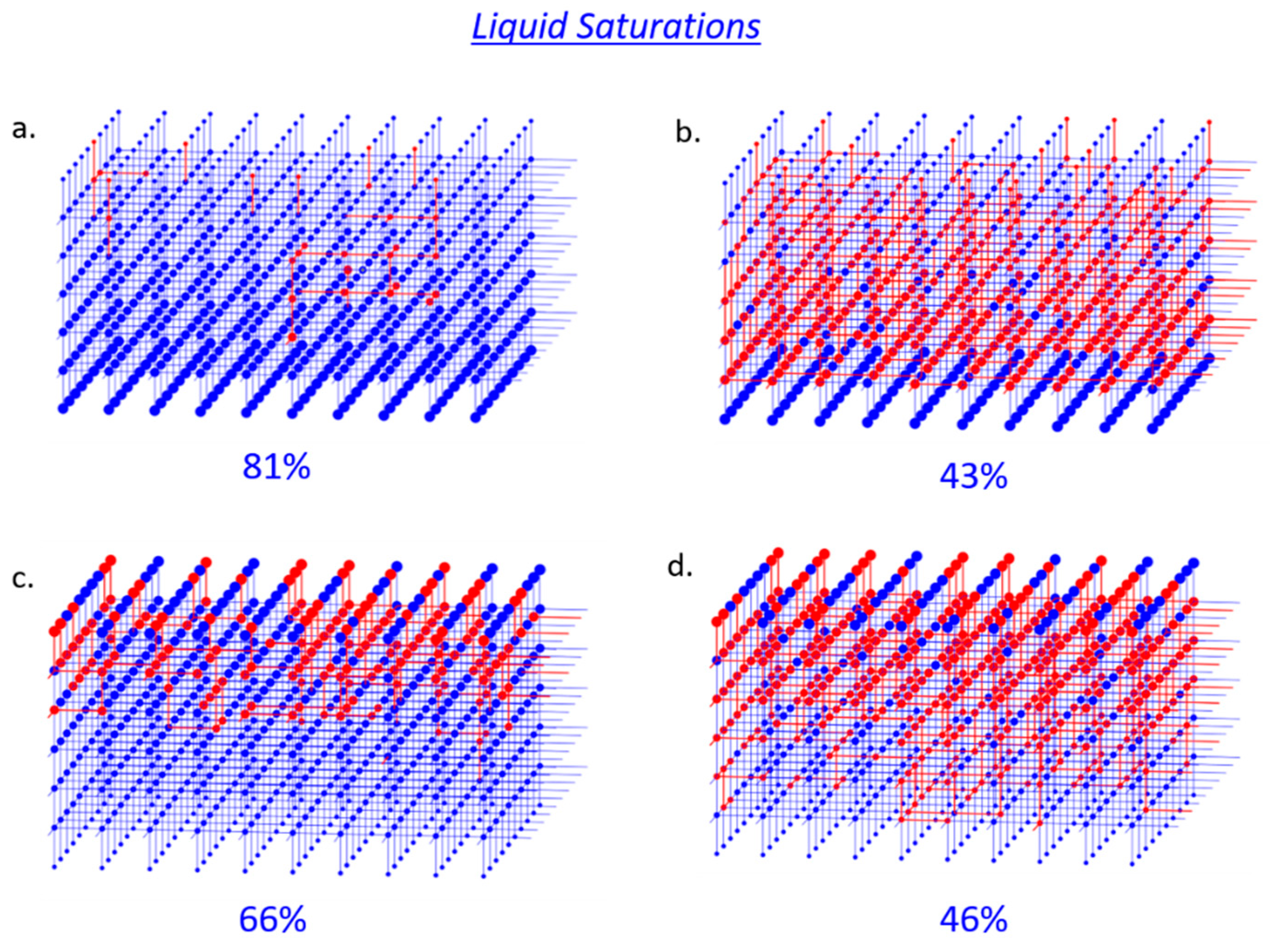
Phase patterns of (a) the LTH gradient at the breakthrough point, (b) the LTH gradient at the water disconnection point, (c) the HTL gradient at the breakthrough point, and (d) the HTL gradient at the water disconnection point. Note that the bottom rows (first pore and throat layers) are not invaded due to the applied cluster labeling rules. Due to this, breakthrough denotes the invasion of the first pore in the second pore row. The figures in (a–d) are from one pore–throat configuration for each case. The saturation values denote the percentage of saturation with the liquid phase.
Figure 11.
Phase patterns of (a) the LTH gradient at the breakthrough point, (b) the LTH gradient at the water disconnection point, (c) the HTL gradient at the breakthrough point, and (d) the HTL gradient at the water disconnection point. Note that the bottom rows (first pore and throat layers) are not invaded due to the applied cluster labeling rules. Due to this, breakthrough denotes the invasion of the first pore in the second pore row. The figures in (a–d) are from one pore–throat configuration for each case. The saturation values denote the percentage of saturation with the liquid phase.

Figure 12.
Saturation profiles summarized for (a) LTH and (b) HTL 3D simulations. The graphs were obtained from Monte Carlo simulation of 15 variations of the pore networks using the simulation parameters summarized in Table 1.
Figure 12.
Saturation profiles summarized for (a) LTH and (b) HTL 3D simulations. The graphs were obtained from Monte Carlo simulation of 15 variations of the pore networks using the simulation parameters summarized in Table 1.

Figure 13.
Comparison of (a) relative liquid and (b) gas permeabilities of LTH and HTL 3D pore networks corresponding to Figure 11. The breakthrough points denote the breakthrough of the gas phase to the second pore row of the pore networks. The absolute permeabilities computed for the empty networks are = 1.24 × 10⁻¹² m2 (LTH) and = 1.38 × 10⁻¹² m2 (HTL).

Figure 14.
(a) Phase patterns and (b) saturation profiles of a 3D pore network with dual porosity (similar as in Figure 2).
Figure 14.
(a) Phase patterns and (b) saturation profiles of a 3D pore network with dual porosity (similar as in Figure 2).

Figure 15.
Permeability of (a) liquid and (b) gas phases in the dual-porosity pore network from Figure 14. The green line in (a) represents the LTH case from Figure 13. The absolute permeability computed for the empty network is = 5.01 × 10⁻¹³ m2 (dual-porosity network).

Figure 16.
Dynamics of the normalized oxygen concentration profile in the liquid phase. Here, denotes the dimensionless concentration of oxygen in the vertical direction, z is the space coordinate, and t is the time.
Figure 16.
Dynamics of the normalized oxygen concentration profile in the liquid phase. Here, denotes the dimensionless concentration of oxygen in the vertical direction, z is the space coordinate, and t is the time.


Table 1.
Overview of simulation parameters.
| 2D | 3D | |
|---|---|---|
| Network size (columns and rows) | 80 10 | 10 10 7 |
| Number of pore network slices | 8 | 5 |
| Number of pores | 800 | 700 |
| Number of throats | 1360 | 1600 |
| Average pore diameter range | (30 to 33.5) µm ± 4 µm | (30 to 32) µm ± 4 µm |
| Average throat diameter range | (22 to 29) µm ± 6 µm | (22 to 26) µm ± 6 µm |
| Lattice spacing | 50 µm | 50 µm |
| Thickness of network | 500 µm | 350 µm |
| Maximum porosity range | 45–65% | 30–50% |
© 2020 by the authors. Licensee MDPI, Basel, Switzerland. This article is an open access article distributed under the terms and conditions of the Creative Commons Attribution (CC BY) license (http://creativecommons.org/licenses/by/4.0/).
Share and Cite
MDPI and ACS Style
Vorhauer-Huget, N.; Altaf, H.; Dürr, R.; Tsotsas, E.; Vidaković-Koch, T. Computational Optimization of Porous Structures for Electrochemical Processes. Processes 2020, 8, 1205. https://0-doi-org.brum.beds.ac.uk/10.3390/pr8101205
AMA Style
Vorhauer-Huget N, Altaf H, Dürr R, Tsotsas E, Vidaković-Koch T. Computational Optimization of Porous Structures for Electrochemical Processes. Processes. 2020; 8(10):1205. https://0-doi-org.brum.beds.ac.uk/10.3390/pr8101205
Chicago/Turabian StyleVorhauer-Huget, Nicole, Haashir Altaf, Robert Dürr, Evangelos Tsotsas, and Tanja Vidaković-Koch. 2020. "Computational Optimization of Porous Structures for Electrochemical Processes" Processes 8, no. 10: 1205. https://0-doi-org.brum.beds.ac.uk/10.3390/pr8101205
Note that from the first issue of 2016, this journal uses article numbers instead of page numbers. See further details here.