Material Requirements Planning Using Variable-Sized Bin-Packing Problem Formulation with Due Date and Grouping Constraints


Department of Systems and Control, Jožef Stefan Institute, 1000 Ljubljana, Slovenia
*
Author to whom correspondence should be addressed.
Processes 2020, 8(10), 1246; https://0-doi-org.brum.beds.ac.uk/10.3390/pr8101246
Submission received: 17 August 2020
/
Revised: 19 September 2020
/
Accepted: 28 September 2020
/
Published: 2 October 2020
(This article belongs to the Special Issue Expanding the Horizons of Manufacturing: Towards Wide Integration, Smart Systems and Tools)
Abstract
:Correct planning is crucial for efficient production and best quality of products. The planning processes are commonly supported with computer solutions; however manual interactions are commonly needed, as sometimes the problems do not fit the general-purpose planning systems. The manual planning approach is time consuming and prone to errors. Solutions to automatize structured problems are needed. In this paper, we deal with material requirements planning for a specific problem, where a group of work orders for one product must be produced from the same batch of material. The presented problem is motivated by the steel-processing industry, where raw materials defined in a purchase order must be cut in order to satisfy the needs of the planned work order while also minimizing waste (leftover) and tardiness, if applicable. The specific requirements of the problem (i.e., restrictions of which work orders can be produced from a particular group of raw materials) does not fit the regular planning system used by the production company, therefore a case-specific solution was developed that can be generalized also to other similar cases. To solve this problem, we propose using the generalized bin-packing problem formulation which is described as an integer programming problem. An extension of the bin-packing problem formulation was developed based on: (i) variable bin sizes, (ii) consideration of time constraints and (iii) grouping of items/bins. The method presented in the article can be applied for small- to medium-sized problems as first verified by several examples of increasing complexity and later by an industrial case study.
1. Introduction
Presently, production and logistics processes are commonly supported with production planning and control systems. These are used to support a range of operational activities from production planning to the detailed scheduling and execution of every operation [1,2,3]. However, it frequently happens that the implemented systems do not adequately cover the problem in a holistic manner. Classical hierarchical organization of the business and production management [4] limits more detailed and tight coupling across the production levels. In practice, different activities of production are supported with separate information systems. Limited data and functional integration among them and additional specifics of the production processes require development and integration of tailor-made solutions.
A holistic view of the production problems become even more important when the environmental footprint of the production is in question. Plant-wide production supervision through data integration and analytics lead to processes that are more effective and consequently the resource demand is reduced. This can even be scaled up by data-sharing and active collaboration with the supply chain, in order to reduce erroneous delivery and consequent undesirable events at the manufacturer’s premises such as stoppage of assembly line [5]. On the other hand, evolution from linear business models to circular economy principles will impose novel problems and dilemmas, such as, for example, strategic planning on supply chain level [6] or remanufacturing pricing strategies [7]. All this requires manufacturers to efficiently schedule, manage and optimize resource consumption of their production processes.
The main motivation of the presented work is the problem faced by the steel-processing manufacturer, where specific requirements for the material requirements planning (MRP) could not be implemented by standard solutions, since the purchasing and planning activities are not supported with the same information system. Consequently, manual interactions are needed which are problematic due to the occurrence of human errors, which are inevitable in the case of more complex situations. In addition, in this way it is almost impossible to produce optimal solutions even for simple problems.
The problem and its specifications originate from steel-processing production, where many products with complex MRP structures are being produced. In principle, raw materials must be cut to satisfy the needs for the input material (intermediates) as defined with MRP. The main requirement of the addressed problem is to plan and optimize material requirements while ensuring that a group of work orders for one final product must be produced from the same batch of raw material. Additionally, it is desirable to limit the tardiness and to reduce the material leftover (small material leftovers lead to a scrap). A custom solution is needed that allows for holistic considerations of purchase and work orders. In practice, optimization systems that holistically address the problem and integrate planning and scheduling are needed, where more adopted solutions are based on mathematical models (e.g., [8]).
The addressed problem of material planning and optimization can be translated into a general bin-packing optimization problem, which has been studied since the early 1970s [9,10]. In the bin-packing problem (BPP), we have m items and n identical bins. The goal is to assign each item to one bin so that the total size of the items in each bin does not exceed the capacity of the bin and the number of bins used is minimized. Different variants of the problem continue to attract researchers’ attention.
The bin-packing problem can be described as an integer optimization problem. Solving the problem is NP-hard and is usually done with custom heuristics. A detailed review of mathematical models and exact algorithms for bin-packing and cutting stock problems are given in [11]. Coffman et al. [12] present an overview of BPP approximation algorithms. However, advances in computer technology and available solver capabilities enables us to solve mid-sized practical problems [13].
The classical problem has been extended to various forms to mitigate many practical application problems. For a general survey see Wäscher et al. [14]. In manufacturing industries, such as in cutting steel, paper or textiles, a cutting stock problem formulation is used. Here, stock material must be cut into shorter lengths to meet demand while minimizing waste. The problems have an identical structure in common [14]. In this context, Carvalho [15] reviewed several linear programming (LP) formulations for the one-dimensional cutting stock and bin-packing problems.
A natural generalization of the classical bin-packing problem is to consider the problem with two or more dimensions. Lodi et al. [16] discussed mathematical models and survey classical approximation algorithms, heuristic and metaheuristic methods, and exact enumerative approaches for 2-D problems. Epstein et al. [17] studied the oriented multi-dimensional dynamic bin-packing problem for two, three, and multiple dimensions. A more general and realistic model considers bins of differing capacities [18]. Bin-packing problem and its variations are still widely studied [19,20]. Recently, Jansen and Kraft [21] presented a review of a variable bin-sized bin-packing problem and an improved approximation scheme to solve the problem.
A bin-packing formulation is also often used to formally represent problems where time must be considered to be well (e.g., scheduling). A simple case is where a task’s durations are represented by items and a job’s due dates with bin sizes. Advanced solutions use the due date as an additional constraint factor. Another solution is to soften the due date constraint, which can be violated but penalized proportionally with the delay. In this context, Reinertsen and Vossen [22] have proposed optimization models and solution procedures that solve the cutting stock problem when orders have due dates. The objective in their model is to minimize scrap and tardiness. Recently, Arbib and Marinelli [23] considered a problem, where each item representing a job must be assigned to a minimum number of bins (resources). Additionally, each item is due by a particular date, so minimal tardiness is also being optimized.
The problem we are targeting arises from the steel-processing production process, where specific constraints must be considered. In this kind of industry even small improvements in the production operation can result in large monetary savings [24]. In our case raw materials are ordered and delivered in batches. Depending on the raw material delivery time, there are some minor variations in the visual properties of the raw material. This may result in a final product that is produced of materials with different properties causing unwanted, additional, repair costs. Therefore, a solution is needed that supports the production planner with decisions on how to cut the available raw materials and how to plan new purchase orders in order to obtain production material as to realize work orders, i.e., final products. The plan must consider various constraints such as the quantity, due dates, single material batch constraints, etc. To support the production planner in dealing with this problem, various generalizations of the classical BPP formulation are proposed. The problem can be designated as an one-dimensional multiple bin-size bin-packing problem (MBSBPP) using the topology of Wäscher et al. [14]. A simple bin-packing problem (BPP) formulation using variable bin sizes and strict time constraints is used when the raw material is available on time. For the case when some of the purchase orders are late, we propose using an upgraded Reinertsen’s optimization model [22]. Soft constraints are introduced into the linear integer problem as proposed in a work of Srikumar [25]. Main contribution of the article is the formulation of specific optimization problem for the problem where group of work orders for one product have to be produced from the same batch of raw material as one batch of raw material consists of several material stocks, which have in common several immeasurable characteristics. Moreover, the problem had to consider the availability of the materials, order deadlines and must minimize the scrap. This is done through introduction of a custom formulation of the bin-packaging problem with constraints that groups the items and bins in a way that assures a consistent final product, while respecting other constraints as well.
In the next section, the general problem formulation is developed step-by-step. Whole or part of the formulation can be used depending on the problem at hand. A model description of the classical bin-packing problem is extended with variable bin sizes, due date constraints, and grouping of bins and items. In Section 3, two case studies are presented that illustrate the practical implementation of the proposed method. Finally, developed methodology and results are discussed in Section 4.
2. Materials and Methods
The problem of material requirements planning can be formalized as a bin-packing problem, which can be solved using a mixed-integer linear program (MILP). In this section, we describe how a basic BPP can be extended to include constraints such as variable bin and item sizes, time limitations, and the fact that only a group of bins can be used to produce one group of items.
2.1. Mathematical Notations
For a consistent discussion, we first define symbolic notation that is consistently used across different mathematical models:
- —decision variable for bin i (1 used, 0 not used)
- —decision variable—item j assignment to bin i (1 assigned, 0 not assigned)
- —soft constraint criteria—tardiness of bin i depending on item j
- I—set of m items (input material defined with work orders)
- B—set of n bins (raw material defined with purchase orders)
- —number of item groups
- —number of bin groups
- —set of items
- —set of bins
- —item (input material) size
- —bin (raw material) size
- —item due date
- —bin delivery time
- —optimization weighting parameters
- —k-th item group
- —l-th bin group
- —number of items in k-th item group
- —number of bins in l-th bin group
2.2. Problem Description
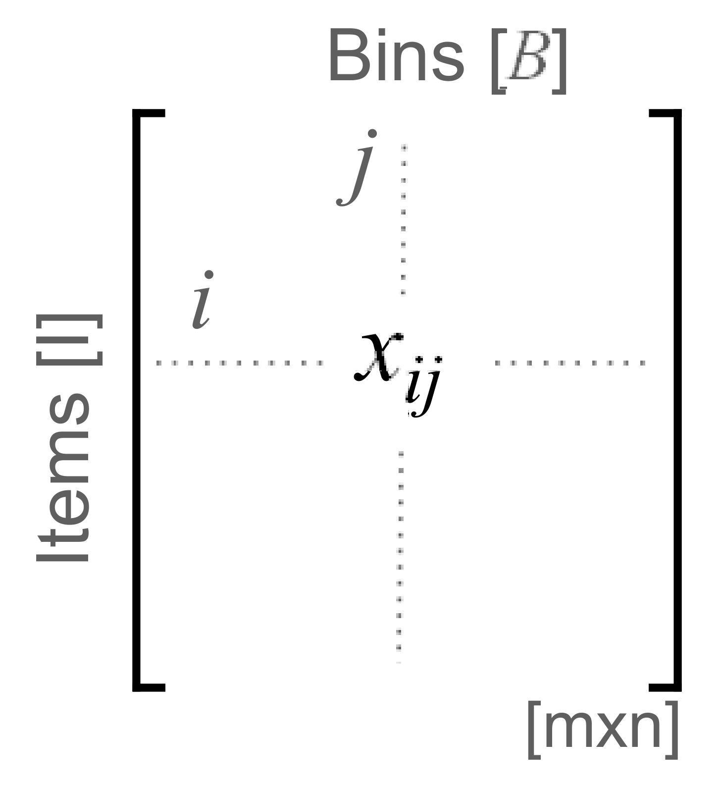
In the classical BPP, we are dealing with a set I of m items, each with its size that has to be assigned to a set B of n identical bins with capacity c. The number of used bins must be minimized, where the sum of item sizes in one bin does not exceed the bin capacity. The problem can be described as an integer optimization problem, as shown in Equation (1).
where and are binary decision variables
Decision variable can be represented as a matrix, depicted in Figure 1.
The first constraint from Equation (1) guarantees that the sum of item sizes assigned to bin does not exceed its capacity, c. The second constraint assures that one item is assigned only to one bin.
2.3. Variable Bin Sizes
There are situations where bin sizes are not identical. Variable bin sizes are denoted as in our work. A set of items can be assigned to bin if the total volume of these items does not exceed the capacity of a bin . For this reason, the first constraint in Equation (1) should be rewritten as given in Equation (2).
The best way to use a bin is to fill it fully, i.e., there is no leftover space. In case of unique bin capacities, the criterion described in Equation (1) minimizes the number of used bins together with the non-assigned capacity of used bin(s)—leftovers. However, this is usually not the case when we have bins of different capacities. In that case, the optimization criteria must be defined as given with Equation (3), where the sum of leftovers of all used bins is being minimized.
2.4. Time Extension
To take into account the time limitations, the problem needs to be additionally extended. The optimization problem needs to consider the situations where bin has to be available before the due date of an item , which is to be scheduled in . The item is therefore defined with a tuple of two elements , where is its due date. Similarly, bin is defined as , where is its delivery time. We suggest two solutions: (i) considering hard (strict) time constraints, where must be available before the due date of () and (ii) considering soft time constraints, where delivery dates are allowed to exceed due dates, but this is penalized within the objective function.
The solution where due date violations are not allowed is achieved with the addition of the following constraint to our optimization problem:
In practice, the due date constraint violation is commonly allowed, but penalized. In this case, we must consider a slightly different problem formulation. The due date constraint must be considered to be a soft constraint. For this reason, we need to first introduce additional tardiness criteria (), which is used to soften the constraint from Equation (4):
If the hard constraint is violated, evaluates the time for which bin is late for item . When there is no delivery time violation, should be 0. Using this, we can extend our criterion function, where we allow that bin can be late. In this way, tardiness is being minimized in addition to leftovers.
As we are dealing here with a multi-objective problem, the weighting of parameters and is introduced, which is used to adjust the importance of leftovers and tardiness criteria. Parameter settings are application-dependent.
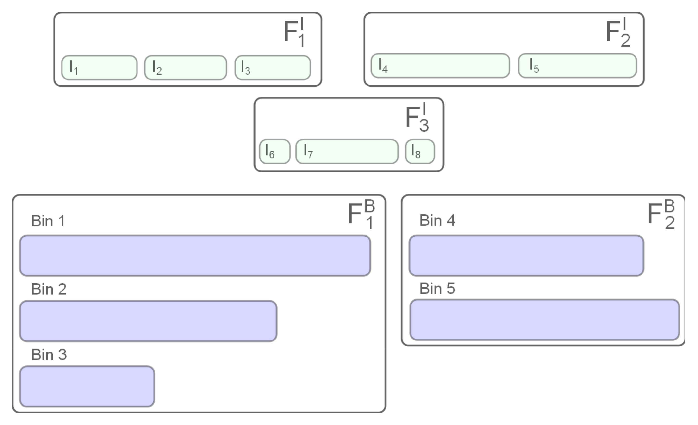
2.5. Grouping of Items/Bins
Furthermore, we are targeting the problem of when a group of items can be assigned to only one single group of bins. This implies additional constraints to our optimization problem.
We assume that we have a set of item groups and set of bin groups. Item is therefore extended to triple , where denotes the group to which item belongs and bin is defined with , where denotes the bin group to which bin belongs. The k-th item group consists of items and l-th bin group consists of bins.
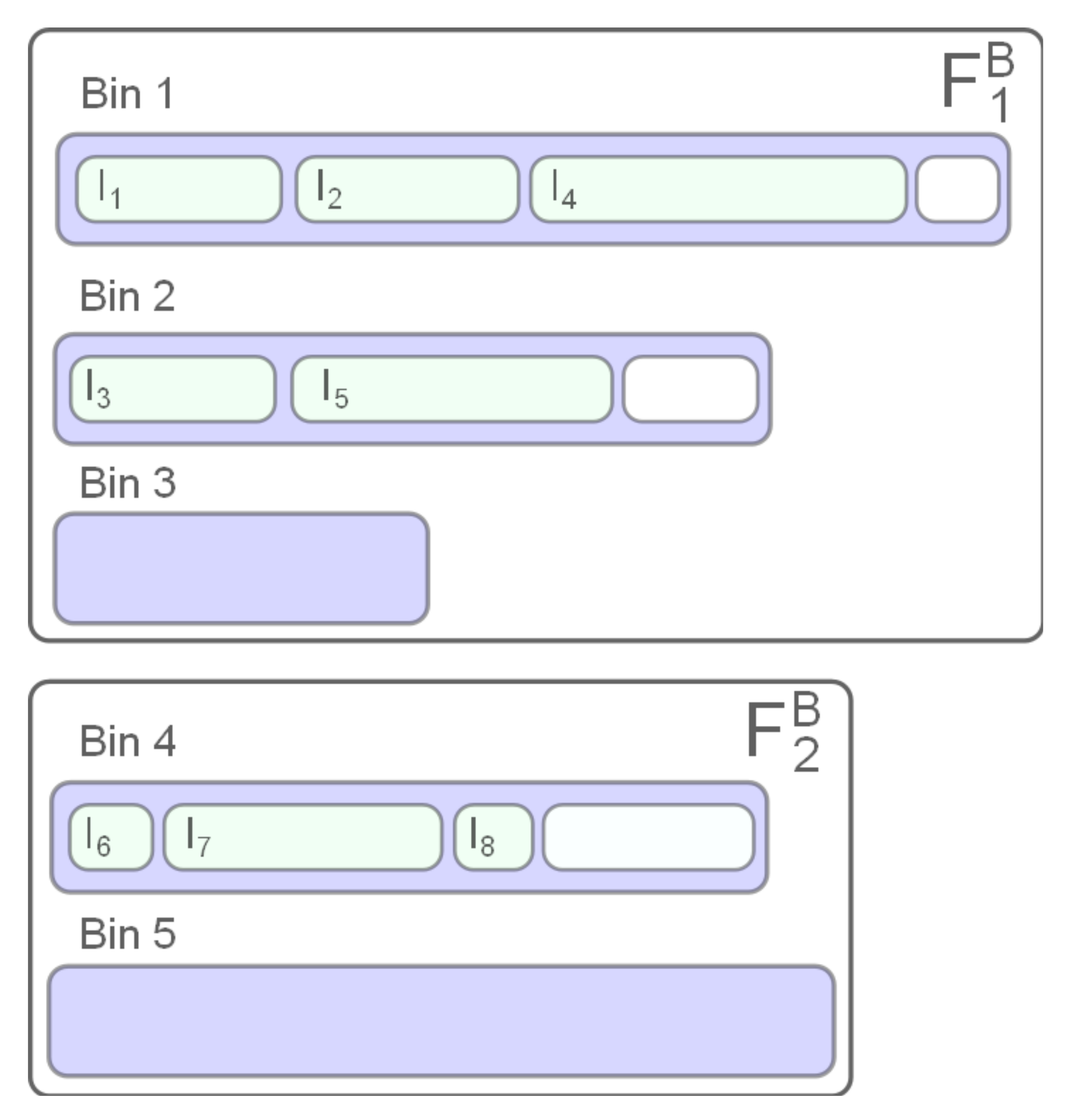
Figure 2 illustrates the example where we have three item groups and two bin groups. Items from one group must be assigned to the bins that are grouped within one bin group. One solution to the problem from the observed example is illustrated in Figure 3. Here items from and are assigned to the bins from bin group , and items from to a bin from bin group . White rectangles indicate the leftovers.
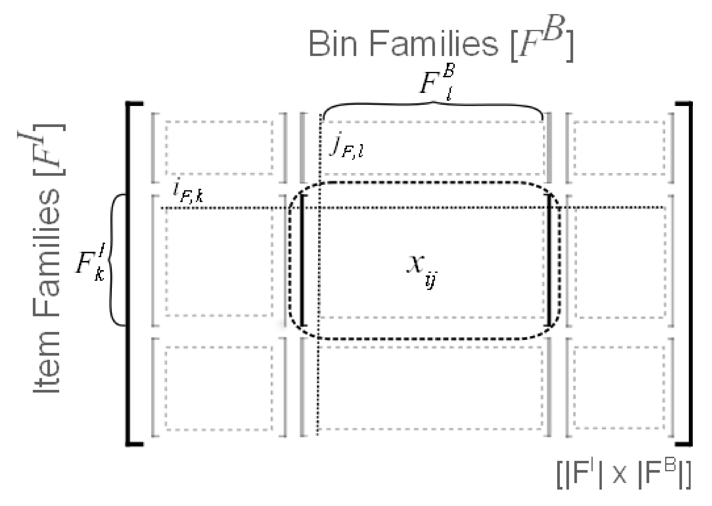
Without loss of the generality, we can assume that the decision variable is organized in a matrix, where items and bins from the same group are given next to each other, as illustrated in Figure 4. Sub-matrices, marked in the figure, indicate all possible group assignments, i.e., combinations of item and bin groups. The items that form k-th item group can be assigned to any of the bins from l-th bin group only if the sum of is equal to the size of item group . Here i designates all items from k-th item group and j all bins from l-th bin group. This can be formally represented by adding the equality constraints (Equation (7)) to our optimization problem from Equation (1).
where … and ….
Here determines the sequence number of the first item in the k-th group of items and is evaluated as:
is the sequence number of the first bin in the l-th group of bins, evaluated as:
Indicator gives information if the combination of bin and item group is used, i.e., it takes a value of 0 or 1. It is defined as a sum of values from submatrix , where the submatrix is defined for all bins from l-th group and only the first item from k-th group. The indicator is implemented as given with Equation (10).
As equality constraints reduce the solution space, the consideration of item and bin grouping constraints actually reduces the complexity of the problem.
3. Results
In this section, the presented BPP problem formulation will be demonstrated in several case studies of material requirements planning with data sets acquired from an industrial environment. All experimental data are available at [26]. The problem concerns raw materials which must be cut to satisfy the needs of work orders for input material. More specifically, raw materials must be available in desired quantities by a specific time, while the input (intermediate) material for one product has to be acquired from the same raw material batch. Purchase orders and work orders are not linked in the current configuration, and material requirements planning is done manually.
Raw materials are provided as defined by purchase orders. In the presented BPP formulation, purchase orders are described with bins, where determine the package size of raw material and the time when it will be available. is not necessarily the same for all raw materials of a particular purchase order. Every purchase order also has a label , which designates a group of raw materials with the same properties. Work orders determine which materials (intermediates) are needed to produce one final product. Every intermediate is presented with an item in our problem formulation, where specifies how much of a material is needed and the work order’s due date. As raw materials can slightly deviate in some parameters, we must deal with additional constraints. We must ensure that a group of intermediates used to make one final product are produced from the same raw material. Label is used to determine items that belong to one work order, i.e., one final product.
In this way, the problem of material requirements planning can be translated into a generalized bin-packing problem. Depending on the situation encountered by the operator, different criterion with different constraints can be applied. We have analyzed two general situations that can occur in practical implementations. If the time constraints are feasible (Equation (4)), then we should apply the optimization problem presented with Equation (3), where the leftover is being minimizing. If this is not possible, softer constraints have to be chosen (Equation (5)), in which we optimize the problem from Equation (6). In this case, we are solving a multi-criterion problem, where leftover and tardiness are being minimized.
3.1. Implementation
The presented case studies were formally described with a mathematical description as defined in Section 2 and implemented with the linear programming modelling environment PuLP [27]. PuLP is an open source high-level modelling library that allows mathematical programs to be described in the Python computer programming language. PuLP provides an interface to many mixed-integer linear programming solvers such as CPLEX, Gurobi, CBC, GLPK. Gurobi solver [28] was used in our case. The solver can offer more algorithms to solve continuous or mixed-integer models. As we are dealing with an integer linear programming problem, we used the dual simplex method.
The problem was solved using a PC with 3.4 GHz and 8 GB RAM.
3.2. Elementary Case Studies
Let us first overview the simplified example introduced in Section 2.5 that illustrates the realistic environment. We must make three products from five available raw materials, which are supplied with two purchase orders. In the generalized BPP formulation, this means that we have two bin groups with five bins:
- ,
- .
Every product is composed of more intermediates. In the generalized BPP formulation, the products are represented with item groups and intermediates with items:
- .
Details about available purchase (bins) and work (items) orders are summarized in Table 1 and Table 2, respectively. We assume here that the processing time needed to cut the raw material is taken into account within .
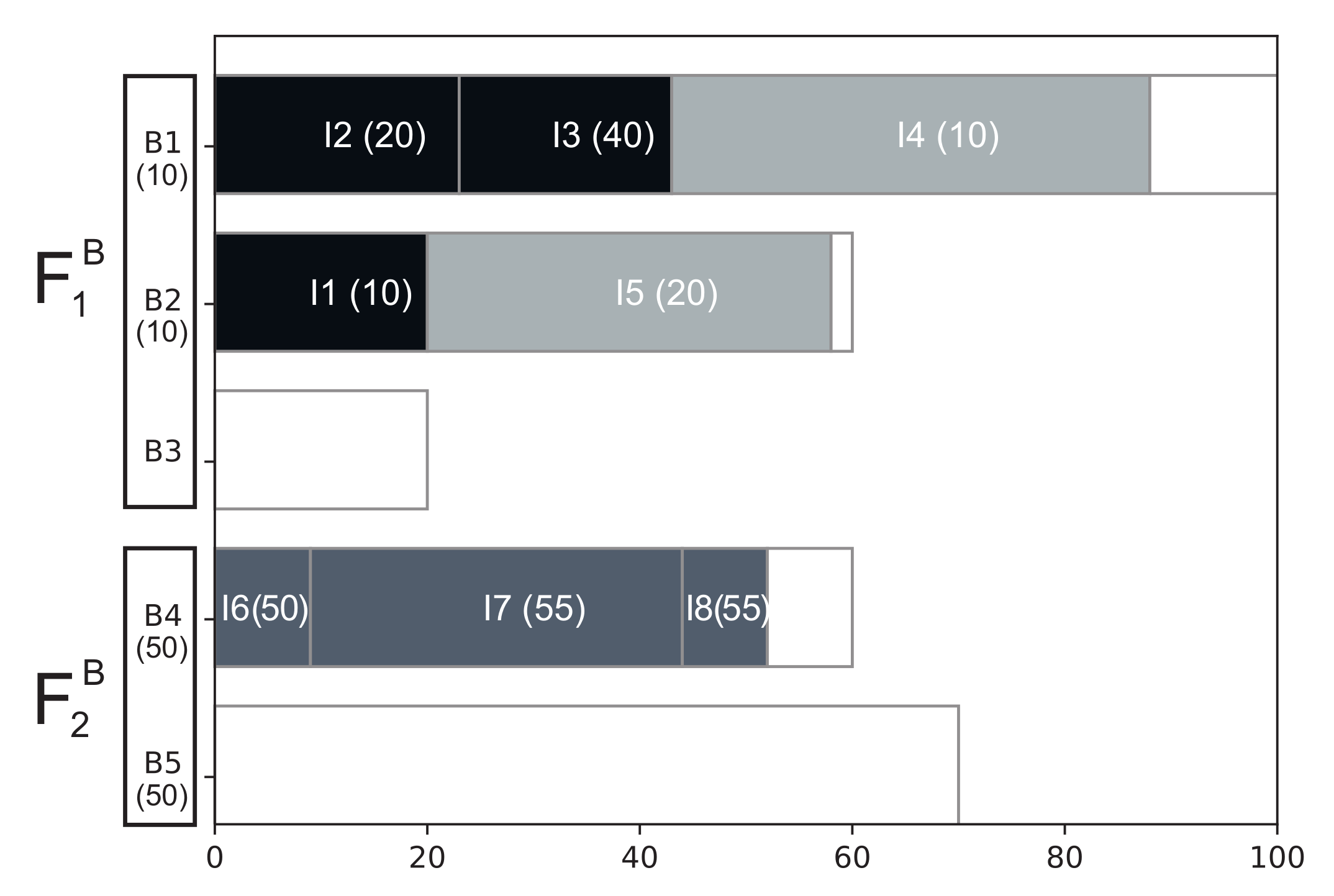
The problem was formulated as an integer optimization problem as described in Section 2 and can be solved without delays, as a solution exists that provides intermediate materials before the time is due. Therefore, we are minimizing the leftover only (Equation (3)). The solver finds an optimal solution, which is graphically presented in Figure 5. The figure shows which intermediates (items) are allocated to a specific purchase order (bin). Next to the bin/item label, time information / are given in round parentheses. Bins that belongs to one bin group are framed together. Items from one group are designated with the same color and we can see that the items from item groups and are assigned to bins from group , while items from are assigned to bin from . Here white rectangles represent the leftovers. Bins , and still have 12, 2 and 8 units of unused space, i.e., the cumulative leftover is , while bins and are not used in a resulting plan.
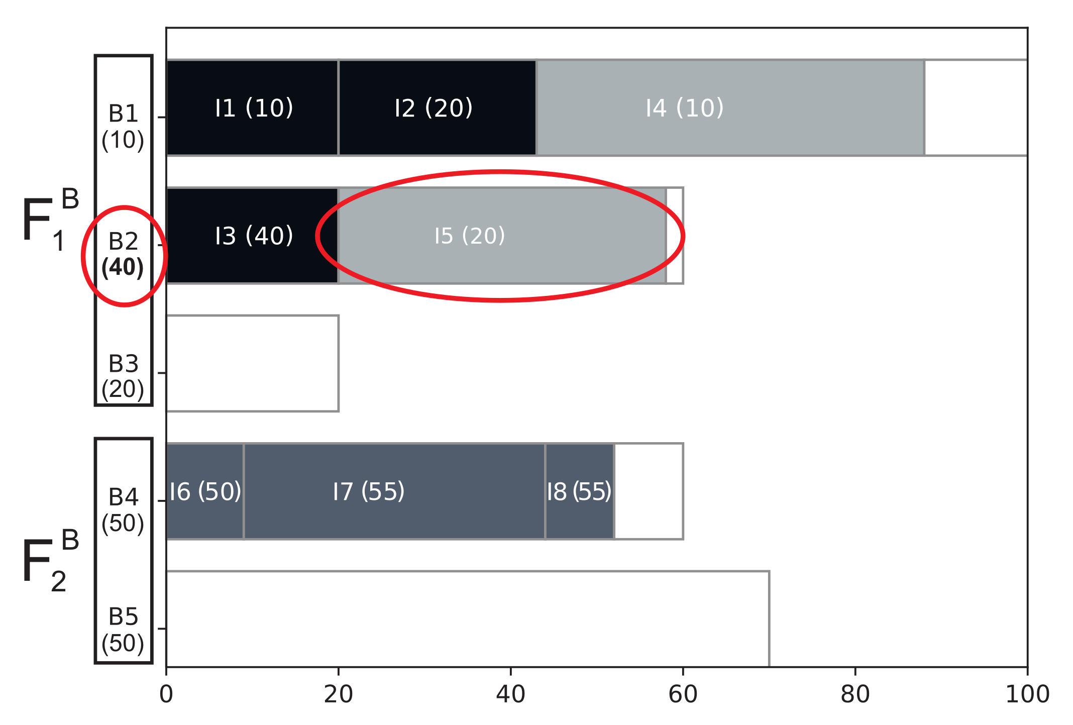
In practice, it often happens that one or more raw material deliveries are delayed, or the product would need to be finished earlier. That type of situation could be illustrated when considering a problem where raw material modelled with bin is late for 30 time units (; all other conditions remain the same). In this case, we cannot achieve a feasible solution using Equation (3). Therefore, an optimization function where delays are allowed but penalized must be used. The multiple criterion function with soft constraints is used to optimize leftover and due date violation (Equation (6)). As for the given problem where tardiness and leftover are equally important, we set the weighting factors as and . Figure 6 shows the resulting schedule where three raw materials (bins) are used and each of them produces some leftover (, and ). We can see that item is planned to be made of bin , which is late for 20 time units (see red designation in Figure 6). The resulting objective function is . Cumulative leftover is the same as in the previous example; however items and are scheduled vice versa in order to minimize total tardiness.
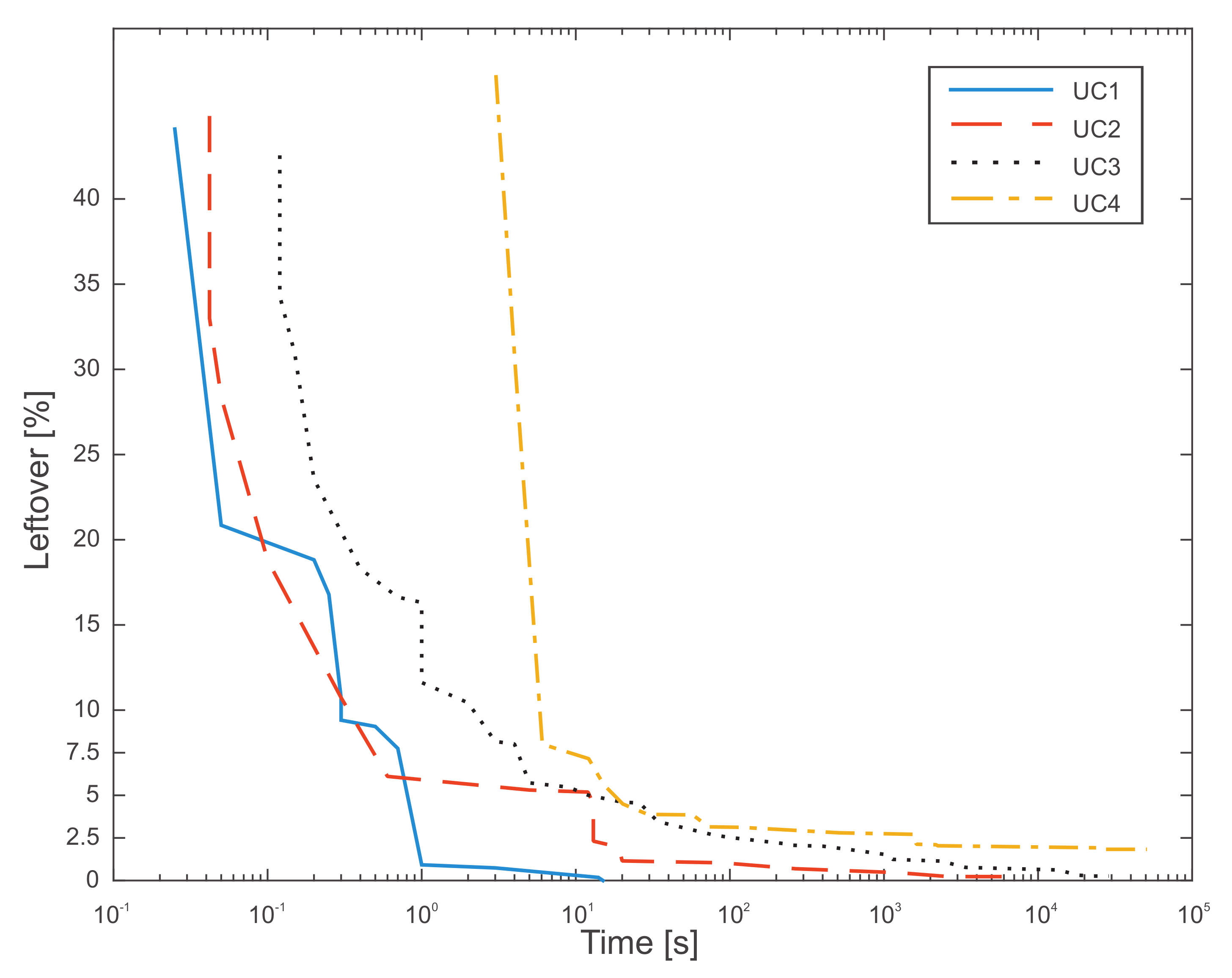
To ensure that the optimization problem works well for large size instances the mathematical formulation of the problem was validated on larger use case problems. Synthetical datasets of four different complexities were generated (UC1–UC4), where in each use cases all the bins are available before item’s due date and for each use case at least one optimal solution, where no leftover is produced. Items and bins for each use case were generated based on optimal solution, where approximately bin groups were used, where in each bin group one bin is left empty. The complexities of the use cases are as follows:
- UC1: 36 items (9 item groups) with 14 bins (5 bin groups). Optimal solution uses 7 bins. Also, the calculated solution uses 7 bins and no leftover is produced.
- UC2: 78 items (9 item groups) with 28 bins (7 bin groups). Optimal solution uses 17 bins. The calculated solution achieved in 44 min uses 16 bins with leftover of 2 units.
- UC3: 125 items (20 item groups) with 52 bins (9 bin groups). Optimal solution uses 29 bins. The calculated solution achieved in 6 h uses 30 bins with leftover of 5 units.
- UC4: 284 items (42 item groups) with 83 bins (16 bin groups). Optimal solution uses 57 bins. The calculated solution achieved in 7 h uses 55 bins with leftover of 60 units.
Figure 7 illustrates how the optimizer converges to optimal solution. For ease of comparison, the leftover is given in percentage of total items capacity. We can see that we achieve solutions with less than 5% of leftovers in a few seconds even for more complex problems that are present in the considered industrial environment. Such a result is incomparably better than can be achieved with the current planning practice. Let us add that such a plan is flawless (no mistakes and no overlapping activities), with fewer leftover and can be continuously upgraded in case of unexpected changes (e.g., new orders).
3.3. Case Study of a Steel-Processing Production Process
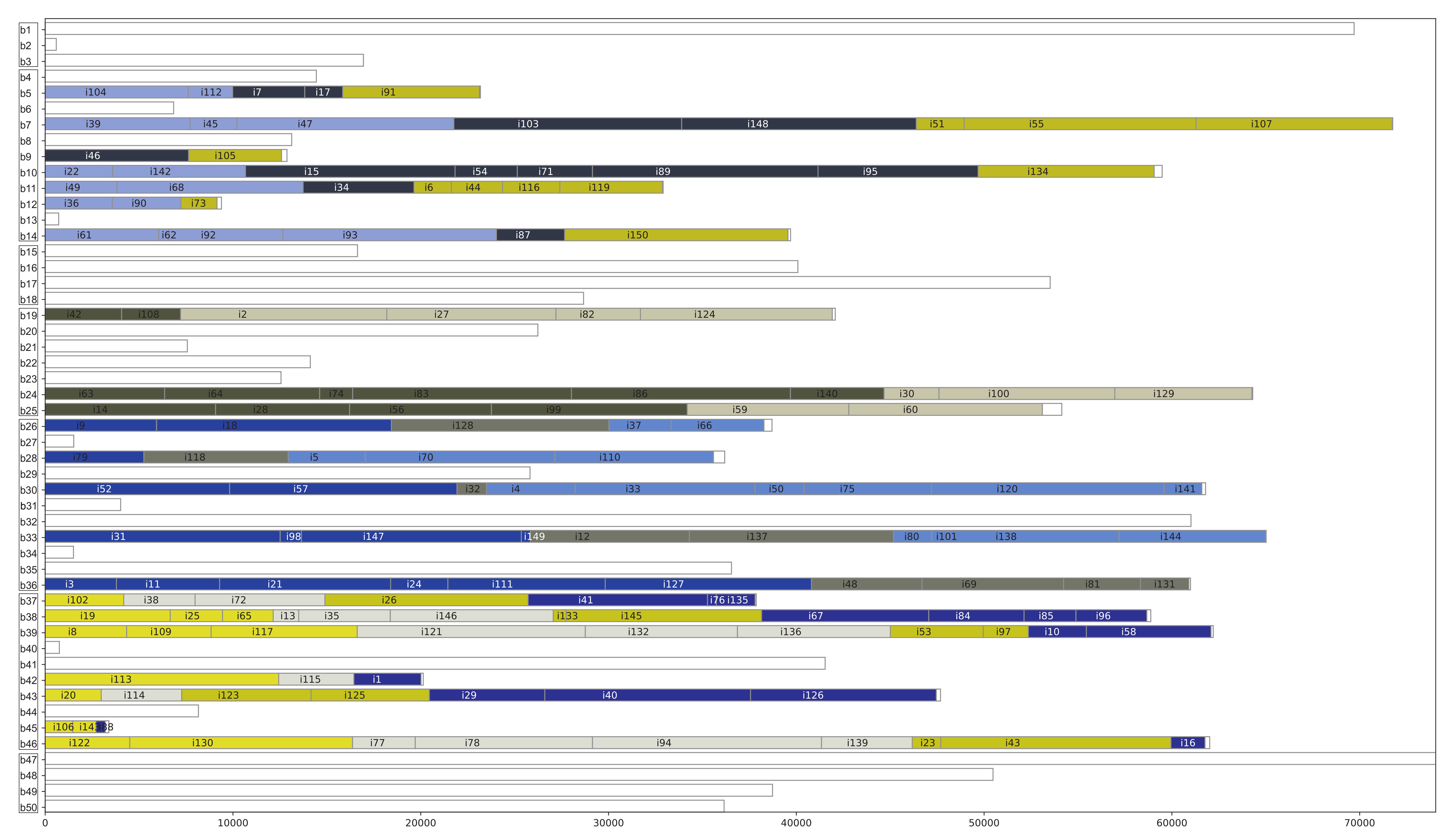
The method is demonstrated on a data set from a real case study and illustrates a common situation in the observed production company. Typically, the production planner must deal with up to 150 intermediates that have to be produced from up to 50 raw materials. In this study, a problem where 150 intermediates (defined with 12 work orders, i.e., item groups) have to be produced from 100 raw materials grouped in 7 bin groups is used to validate our modelling and problem solving capabilities.
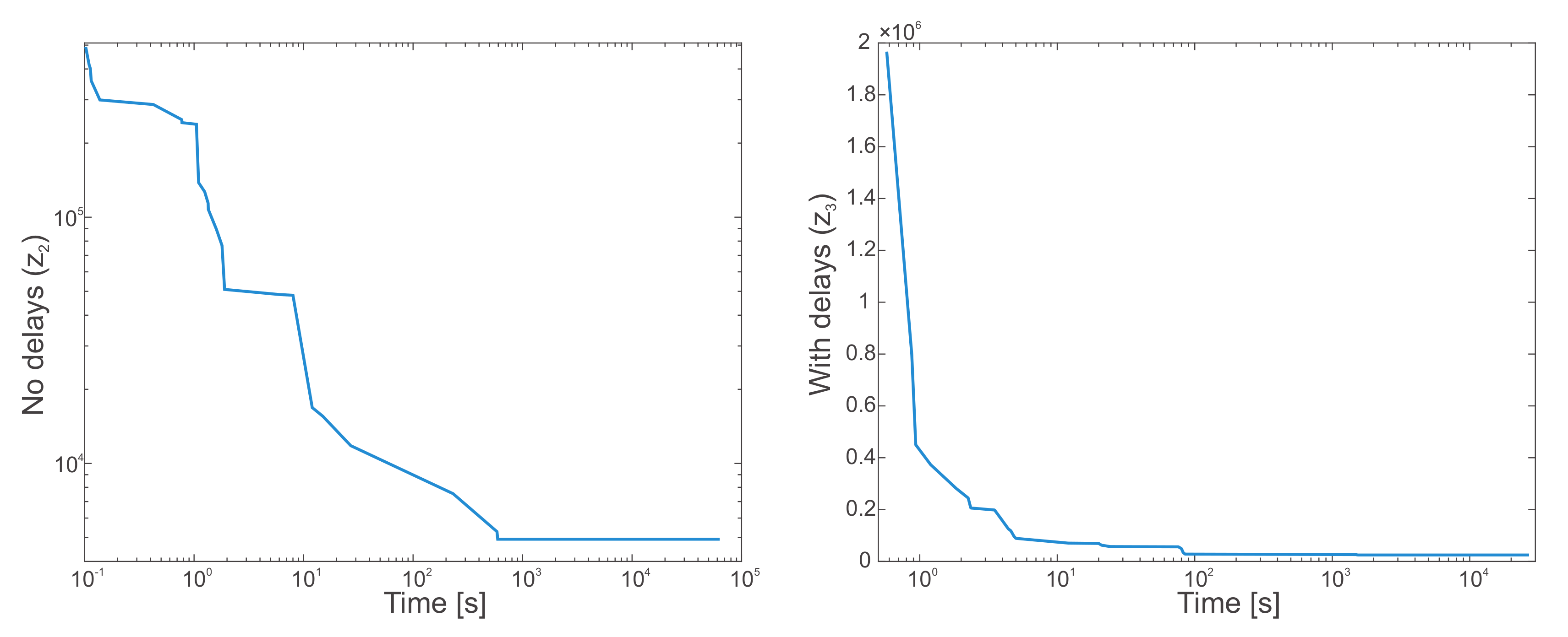
The problem was modelled and solved with the same procedure as described in the simple case study (criterion function from Equation (3)). As the problem is NP-hard, it is not possible to achieve the optimal solution in a short time. In our case, it took 593 s to achieve a close to optimal solution. The graph on the left of Figure 8 illustrates how the optimizer converges to an optimal solution. We do not achieve a better solution even if the optimization is run for a much longer time (24 h). The final solution produces 4923 of leftover when 22 bins are used. The solution and resulting plan are presented in Figure 9.
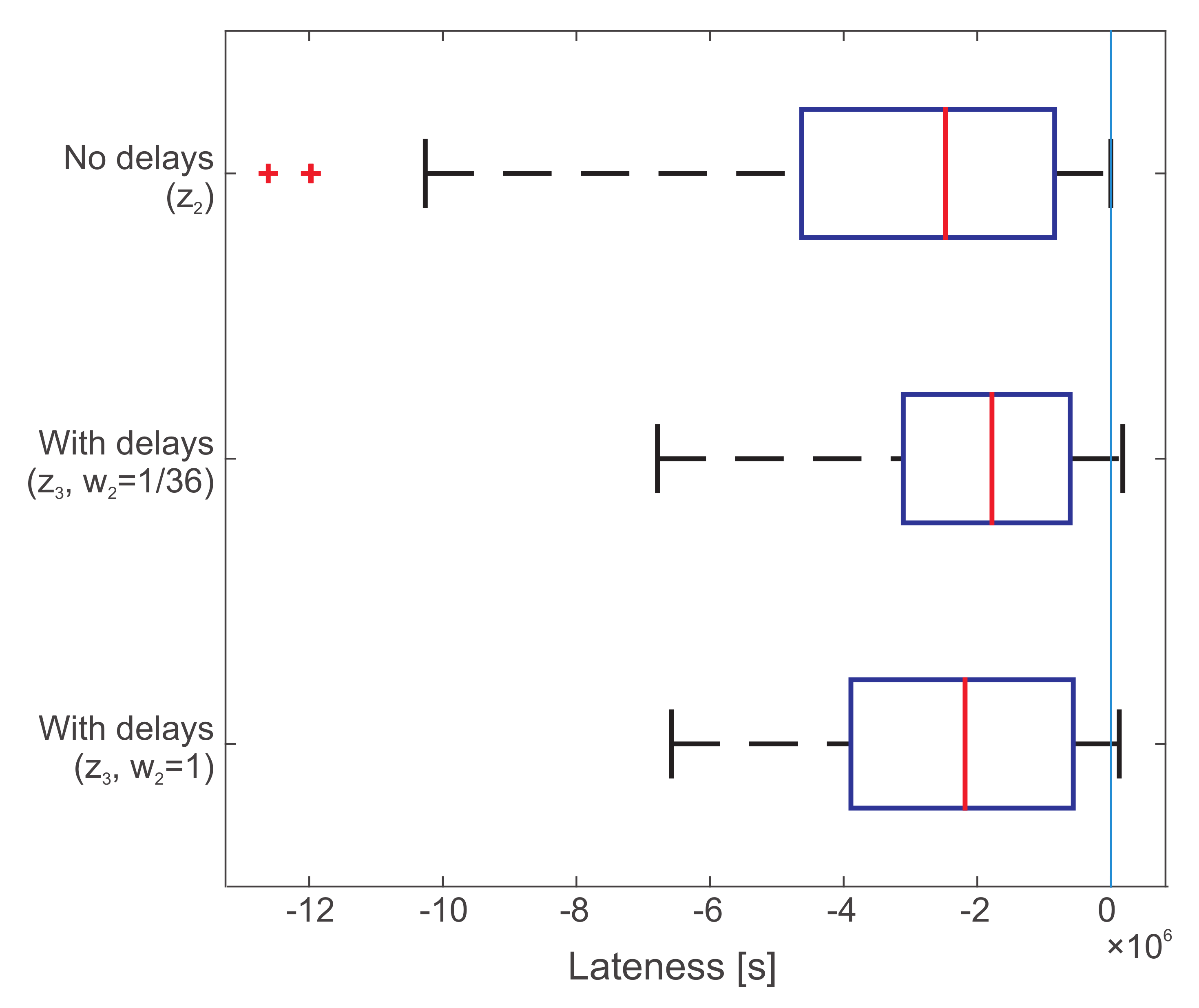
We also analyzed a problem in which two purchase orders are late. In this case, we need to use the criterion function with soft constraints (Equation (6)) to optimize leftover and due date delays simultaneously. The following weighting factor values are considered in this experiment: and . With the given settings, we get a solution () in which 25 bins are used and the cumulative leftover is 4238. In the resulting solution, more items are late. Their cumulative tardiness is 665,012 s, i.e., approximately 7.5 days. In this case, the optimization process took more time (26,518 s). The graph on the right in Figure 8 illustrates how the solution converges in this case. However, a close to optimal solution can be achieved in approx. 100 s.
In the case that minimization of the leftover is more important, we would choose other weighting factors ( and ). In this case, 26 bins are used with a higher leftover of 11,200, but with a lower total tardiness (551,237 s), which means more than one day shorter than in the previous case. In this case, optimization took approximately 157 s.
Figure 10 illustrates the lateness of the work orders for all three studied cases, i.e., positive and negative difference between the completion time and the due date. We can see that none of the work orders are late in the case when purchase orders are available on time (upper data). In the case when two purchase orders are late, we can see that this will cause some work orders to also be late. However, there will be less delays in the case when the tardiness weighting factor is set to .
4. Discussion
General-purpose IT solutions can solve several problems at hand. But often, production specifics require development of special tailor-made solutions. In this paper, we considered a problem from manufacturing in which stock material must be cut to provide a reliable material requirements plan. This plan must satisfy the needs of capacity and must be available by the work order’s due date. Besides this, the plan must also consider the fact that a group of work orders must be produced from the same batch of raw material. In this way, the manufacturer can systematically compensate for some undesirable variations in raw material quality. In the current day to day practice, the plan is managed manually, and it is very difficult to maintain the plan up-to-date, even in smaller dimensions. The decisions of the operator are time consuming and prone to errors. This results in situations in which the operator must constantly make plan corrections.
In this paper, we propose using an extended bin-packing problem formulation to systematically solve the material planning. A basic BPP formulation is extended to include constraints such as variable bin and item sizes, time limitations, and the fact that only a group of bins can be used to produce one group of items.
The suggested solution offers a tool for supporting the production planner with his/her decisions. With it, he/she can determine how to efficiently cut the raw material to satisfy the planned work orders. Depending on the situation, the planner can choose between various model formulations. He/she can optimize the leftover, tardiness, or both.
We demonstrated that the proposed solution can solve a problem of realistic dimensions quickly enough to be used in an industrial application. However, in real applications, case-specific requirements would first need to be analyzed to most appropriately set the importance of leftovers and/or tardiness. In this way, the time for producing a feasible material requirements plan is reduced. The operator is relieved and can be focused on other tasks. Also, the need for corrections is decisively reduced. To summarize, variations in raw material quality no longer cause a problem when implementing our solution. We propose to use a rigorous and accessible MILP solution approach, i.e., Gurobi optimization solver, which satisfies the requirements of the problem considered in this paper. To extend the use of the proposed method to more complex problems approximation algorithms should be applied (e.g., [3,12,21]).
To summarize, variations in raw material properties no longer cause a problem when implementing our solution, since end products are made from the same material and, consequently, the products’ quality is improved. Moreover, raw material batches are used more rationally, which leads to decrease the needed of storage place and unused batch leftovers.
Author Contributions
Conceptualization, methodology, software and validation, D.G. and M.G.; writing–original draft preparation, D.G.; writing–review and editing, M.G. All authors have read and agreed to the published version of the manuscript.
Funding
The work was supported by the INEVITABLE project which has received funding from the European Union’s Horizon 2020 research and innovation program under grant agreement No 869815. The support of the Slovenian Research Agency (P2-0001) is also acknowledged.
Conflicts of Interest
The authors declare no conflict of interest. The funders had no role in the design of the study; in the collection, analyses, or interpretation of data; in the writing of the manuscript, or in the decision to publish the results.
Abbreviations
The following abbreviations are used in this manuscript:
| MRP | Material requirements planning |
| BPP | Bin-packing problem |
| MBSBPP | Multiple bin-size bin-packing problem |
| LP | Linear programming |
| MILP | Mixed-integer linear program |
References
- Onwubolu, G. Emerging Optimization Techniques in Production Planning and Control; Imperial College Press: London, UK, 2002. [Google Scholar]
- Plenert, G. Focusing material requirements planning (MRP) towards performance. Eur. J. Oper. Res. 1999, 119, 91–99. [Google Scholar] [CrossRef]
- De, A.; Choudhary, A.; Turkay, M.; Tiwari, M.K. Bunkering policies for a fuel bunker management problem for liner shipping networks. Eur. J. Oper. Res. 2019, in press. [Google Scholar] [CrossRef]
- ISO/IEC. IEC 62264-3: Enterprise-Control System Integration—Part 3: Activity Models of Manufacturing Operations Management; ISO/IEC: Geneva, Switzerland, 2016. [Google Scholar]
- Goswami, M.; De, A.; Habibi, M.K.K.; Daultani, Y. Examining freight performance of third-party logistics providers within the automotive industry in India: An environmental sustainability perspective. Int. J. Prod. Res. 2020, 1–28. [Google Scholar] [CrossRef]
- Suzanne, E.; Absi, N.; Borodin, V. Towards circular economy in production planning: Challenges and opportunities. Eur. J. Oper. Res. 2020, 287, 168–190. [Google Scholar] [CrossRef]
- Ray, A.; De, A.; Mondal, S.; Wang, J. Selection of best buyback strategy for original equipment manufacturer and independent remanufacturer—game theoretic approach. Int. J. Prod. Res. 2020, 1–30. [Google Scholar] [CrossRef]
- Garcia-Sabater, J.P.; Maheut, J.; Garcia-Sabater, J.J. A two-stage sequential planning scheme for integrated operations planning and scheduling system using MILP: The case of an engine assembler. Flex. Serv. Manuf. J. 2012, 24, 171–209. [Google Scholar] [CrossRef]
- Gilmore, P.C.; Gomory, R.E. A Linear Programming Approach to the Cutting Stock Problem—Part II. Oper. Res. 1963, 11, 863–888. [Google Scholar] [CrossRef]
- Martello, S.; Toth, P. Knapsack Problems: Algorithms and Computer Implementations; John Wiley & Sons, Inc.: New York, NY, USA, 1990. [Google Scholar]
- Delorme, M.; Iori, M.; Martello, S. Bin packing and cutting stock problems: Mathematical models and exact algorithms. Eur. J. Oper. Res. 2016, 255, 1–20. [Google Scholar] [CrossRef]
- Coffman, E.; Csirik, J.; Galambos, G.; Martello, S.; Vigo, D. Bin Packing Approximation Algorithms: Survey and Classification; Springer: New York, NY, USA, 2013; Volumes 1–5, pp. 455–531. [Google Scholar]
- Kim, T. Production Planning to Reduce Production Cost and Formaldehyde Emission in Furniture Production Process Using Medium-Density Fiberboard. Processes 2019, 7, 529. [Google Scholar] [CrossRef] [Green Version]
- Wäscher, G.; Haußner, H.; Schumann, H. An improved typology of cutting and packing problems. Eur. J. Oper. Res. 2007, 183, 1109–1130. [Google Scholar] [CrossRef]
- De Carvalho, J.M.V. LP models for bin packing and cutting stock problems. Eur. J. Oper. Res. 2002, 141, 253–273. [Google Scholar] [CrossRef]
- Lodi, A.; Martello, S.; Monaci, M. Two-dimensional packing problems: A survey. Eur. J. Oper. Res. 2002, 141, 241–252. [Google Scholar] [CrossRef]
- Epstein, L.; Levy, M. Dynamic multi-dimensional bin packing. J. Discret. Algorithms 2010, 8, 356–372. [Google Scholar] [CrossRef] [Green Version]
- Friesen, D.K.; Langston, M.A. Variable sized bin packing. SIAM J. Comput. 1986, 15, 222–230. [Google Scholar] [CrossRef]
- Hemmelmayr, V.; Schmid, V.; Blum, C. Variable Neighbourhood Search for the Variable Sized Bin Packing Problem. Comput. Oper. Res. 2012, 39, 1097–1108. [Google Scholar] [CrossRef]
- Bang-Jensen, J.; Larsen, R. Efficient algorithms for real-life instances of the variable size bin packing problem. Comput. Oper. Res. 2012, 39, 2848–2857. [Google Scholar] [CrossRef]
- Jansen, K.; Kraft, S. An Improved Approximation Scheme for Variable-Sized Bin Packing. Theory Comput. Syst. 2016, 59, 262–322. [Google Scholar] [CrossRef]
- Reinertsen, H.; Vossen, T.W. Discrete optimization. Eur. J. Oper. Res. 2010, 201, 701–711. [Google Scholar] [CrossRef]
- Arbib, C.; Marinelli, F. Maximum lateness minimization in one-dimensional bin packing. Omega 2017, 68, 76–84. [Google Scholar] [CrossRef]
- Maddaloni, A.; Colla, V.; Nastasi, G.; Seppia, M.D.; Iannino, V. A Bin Packing Algorithm for Steel Production. In Proceedings of the 2016 European Modelling Symposium (EMS), Pisa, Italy, 28–30 November 2016; pp. 19–24. [Google Scholar]
- Srikumar, V. Soft Constraints in Integer Linear Programs. Unpublished Note. 2013. Available online: https://svivek.com/research/srikumar2013soft-constraints.html (accessed on 1 October 2020).
- Gradišar, D.; Glavan, M. Data—MRP Using BPP. Available online: https://0-doi-org.brum.beds.ac.uk/10.13140/RG.2.2.27414.98885/1 (accessed on 1 October 2020).
- Mitchell, S.; Kean, A.; Mason, A.; O’Sullivan, M.; Phillips, A.; Peschiera, F. Optimization with PuLP. Available online: https://coin-or.github.io/pulp/ (accessed on 1 September 2020).
- Gurobi. Gurobi Optimizer. Available online: http://www.gurobi.com (accessed on 1 September 2020).
Figure 1.
Decision variable in basic BPP.

Figure 2.
Item and bin groups.

Figure 3.
Item and bin groups. Acceptable solution: and .

Figure 4.
Decision variable - item and bin groups.

Figure 5.
Solution to a simple problem.

Figure 6.
Solution to a simple problem where is late.

Figure 7.
Validation on synthetical datasets (UC1–UC4).

Figure 8.
Convergence of criterion functions for the case study with no delays (left) and with delays (right).
Figure 8.
Convergence of criterion functions for the case study with no delays (left) and with delays (right).

Figure 9.
Resulting MRP plan for the case study with no delays ().

Figure 10.
Lateness of input materials.


Table 1.
Purchase orders—Bins.
| Bin | |||
|---|---|---|---|
| 100 | 10 | 1 | |
| 60 | 10 | 1 | |
| 20 | 20 | 1 | |
| 60 | 50 | 2 | |
| 70 | 50 | 2 |
Table 2.
Work orders—Items.
| Item | |||
|---|---|---|---|
| 20 | 10 | 1 | |
| 23 | 20 | 1 | |
| 20 | 40 | 1 | |
| 45 | 10 | 2 | |
| 38 | 20 | 2 | |
| 9 | 50 | 3 | |
| 35 | 55 | 3 | |
| 8 | 55 | 3 |
© 2020 by the authors. Licensee MDPI, Basel, Switzerland. This article is an open access article distributed under the terms and conditions of the Creative Commons Attribution (CC BY) license (http://creativecommons.org/licenses/by/4.0/).
Share and Cite
MDPI and ACS Style
Gradišar, D.; Glavan, M. Material Requirements Planning Using Variable-Sized Bin-Packing Problem Formulation with Due Date and Grouping Constraints. Processes 2020, 8, 1246. https://0-doi-org.brum.beds.ac.uk/10.3390/pr8101246
AMA Style
Gradišar D, Glavan M. Material Requirements Planning Using Variable-Sized Bin-Packing Problem Formulation with Due Date and Grouping Constraints. Processes. 2020; 8(10):1246. https://0-doi-org.brum.beds.ac.uk/10.3390/pr8101246
Chicago/Turabian StyleGradišar, Dejan, and Miha Glavan. 2020. "Material Requirements Planning Using Variable-Sized Bin-Packing Problem Formulation with Due Date and Grouping Constraints" Processes 8, no. 10: 1246. https://0-doi-org.brum.beds.ac.uk/10.3390/pr8101246
Note that from the first issue of 2016, this journal uses article numbers instead of page numbers. See further details here.