Comparison of Solar Collector Testing Methods—Theory and Practice

Abstract

One of the most important problems of operating solar heating systems involves variable efficiency depending on operating conditions. This problem is more pronounced in hybrid energy systems, where a solar installation cooperates with other segments based on conventional carriers of energy or renewable sources of energy. The operating cost of each segment of a hybrid system depends mainly on the resulting efficiency of solar installation. For over 40 years, the procedures of testing solar collectors have been undergoing development, testing, comparison and verification in order to create a procedure that would allow determining the thermal behavior of a solar collector without performing expensive and complicated experimental tests, usually based on the steady state condition. The proper determination of the static and dynamic properties of a solar collector is of key significance, as they constitute a basis for the design of a solar heating installation, as well as a control system. It is therefore important to conduct simulating and operating tests enabling the performance of a comparative analysis intended to indicate the degree to which the static and dynamic properties of a solar collector depend on the method used for their determination. The paper compares the static and dynamic properties of a flat solar collector determined by means of various methods. Based on the produced results, it has been concluded that the static and dynamic properties of a collector determined using various methods may differ from each other even by 50%. This means that it is possible to increase the efficiency of a solar heating installation via the use of an adaptive control algorithm, enabling real-time calculation of the values of characteristic parameters of solar installation, e.g., the time constant under operating conditions.

Highlights

• Comparison of solar collector testing methods.
• Static and dynamic properties of the collector determined by different methods may differ from each other by up to 50%.
• Increase in the efficiency of the solar installation possible with an adaptive control system.

1. Introduction

One of the main operational problems encountered in solar heating installations involves their considerably lower efficiency reached under operating conditions compared to that assumed at the engineering stage. Despite the use of various techniques based on artificial neural networks [1], genetic algorithms [2] and other stochastic techniques [3] to optimize the operation of the solar heating system, the problem has still not been satisfactorily resolved. The low efficiency problem occurs very often in hybrid power supply systems, in which a solar system cooperates with other heating and cooling plants in a hybrid energy system, e.g., Solar-Assisted Heat Pumps, Ground-Source Heat Pumps, gas and oil heating. Under operating conditions, the thermal behavior of each component of a system has noticeable influence on the thermal behavior of other components, which affects efficiency in particular segments, and, as a result, the efficiency of the whole system.

The operating cost of each segment of a hybrid system depends mainly on the resulting efficiency of a solar installation. In practice, the lower efficiency of a solar system translates into higher consumption of fossil fuel, which generates higher operating costs. Therefore, experimental work is still being carried out on new collector constructions [4] and the possibility of long-term energy accumulation using phase change materials [5], such as trigeneration systems [6]. It is possible to achieve optimization of the operation of a solar installation (solar system capacity increase) using smooth flow control of the working medium that should be adjusted to the existing operating conditions (solar radiation intensity, temperature of the medium, water temperature in the storage tank) [7]. It is possible to develop the control system of a solar segment in a hybrid installation based on the dynamic properties of the solar collector represented by the time constant determined using a step response [8]. For over 40 years, the procedures of testing solar collectors have been undergoing development, testing, comparison and verification in order to create a procedure that would allow determining the thermal behavior of a solar collector without performing expensive and complicated experimental tests, usually based on the steady state condition. The proper determination of the static and dynamic properties of a solar collector is of key significance, as they constitute a basis for the design of a solar heating installation, as well as a control system. In spite of the continuing development of the concepts of adjusting the operation of a solar heating installation based on the simplest proportional controller [9], proportional and on-off fluid flow control algorithm [10], proportional-derivative control algorithm [11], through continuous adjustment using a Proportional Integral Differential PID regulator [12,13] and ending with complicated fuzzy algorithms [14,15], learning algorithm [16], and artificial neural networks [17] improving the performance of thermal solar collector, the ensuring of required control quality still remains an issue. They probably arise from the fact that the static and dynamic parameters of solar collectors determined in laboratory tests can be different under operating conditions. Although the quality standard ISO 9459-4:2013 [18] was developed to test solar heating systems under operating conditions, it does not allow determining the thermal behavior of a solar collector. It is therefore important to conduct simulating and operating tests enabling the performance of a comparative analysis intended to indicate the degree to which the static and dynamic properties of a solar collector depend on the method used for their determination.

2. An Overview of Test Methods for Flat-Plate Solar Collectors

The basic model of a flat-plate solar collector on which the quality standards Ashrae [18], EN12975-1:2010 [19] and ISO9806:2017 [20] are based includes an equation developed by Hottel, Whilier and Bliss (

Table 1. Characteristic parameters for each method and conditions for which it is correct.

Item		Collector Model	Characteristic Parameters of the Collector	Testing Conditions	Method of the Equation Coefficient Estimation	Test Stand	Number of Homogeneous Bodies in the Collector Structure
1	HWB [21]	${\left(\mathrm{mc}\right)}_{\mathrm{e}} \frac{{\mathrm{dT}}_{\mathrm{fo}}}{\mathrm{dt}}={{\mathrm{F}}^{\prime }\mathrm{A}}_{\mathrm{c}}\left[{\left(\mathsf{\tau }\mathsf{\alpha }\right)}_{\mathrm{e}}{\mathrm{I}}_{\mathrm{T}}-{\mathrm{U}}_{\mathrm{L}}\left({\mathrm{T}}_{\mathrm{fm}}-{\mathrm{T}}_{\mathrm{A}}\right)\right]+{\dot{\mathrm{m}}\mathrm{c}}_{\mathrm{p}}\left({\mathrm{T}}_{\mathrm{fi}}-{\mathrm{T}}_{\mathrm{fo}}\right)$	F’(τα), F’UL, ${\left(\mathrm{mc}\right)}_{\mathrm{e}}$	$\dot{\mathrm{m}}$= C, Tfi = C, IT = C	Method of least squares	Specified in the standards	1
2	Roger’s method [22]	${\mathrm{q}}_{\mathrm{u}}\left(\mathrm{j}\right)={\displaystyle \sum _{\mathrm{n}=1}^{\mathrm{N}}}\left[{\mathrm{F}}_{\mathrm{R}}{\left(\mathsf{\tau }\mathsf{\alpha }\right)}_{\mathrm{e}}{ \mathrm{K}}_{\mathrm{n}}{\mathrm{I}}_{\mathrm{j}}\left(\mathrm{n}\right)\right]-{\mathrm{F}}_{\mathrm{R}}{\mathrm{U}}_{\mathrm{L}}\overline{\left({\mathrm{T}}_{\mathrm{f}}-{\mathrm{T}}_{\mathrm{A}}\right)}$	${\mathrm{F}}_{\mathrm{R}}{\left(\mathsf{\tau }\mathsf{\alpha }\right)}_{\mathrm{e}}$, ${\mathrm{F}}_{\mathrm{R}}{\mathrm{U}}_{\mathrm{L}}$	$\dot{\mathrm{m}}$ = C, Tfi = C, IT ≠ C, ${\mathrm{T}}_{\mathrm{A}}$≠ C	Linear regression method	In accordance with the standard	1
3	Saunier’s method [23]	$\left({\mathrm{M}}_{\mathrm{a}}+{\mathrm{M}}_{\mathrm{e}}\right){\mathrm{c}}_{\mathrm{p}}\frac{\partial {\mathrm{T}}_{\mathrm{fm}}}{\partial \mathrm{t}}={\mathsf{\eta }}_0{\mathrm{A}}_{\mathrm{p}}{\mathrm{I}}_{\mathrm{T}}-\left({\mathrm{a}}_1+{\mathrm{U}}_{\mathrm{a}}\right){\mathrm{A}}_{\mathrm{p}}\left({\mathrm{T}}_{\mathrm{fm}}-{\mathrm{T}}_{\mathrm{A}}\right)-{\mathrm{a}}_2{\mathrm{A}}_{\mathrm{p}}{\left({\mathrm{T}}_{\mathrm{fm}}-{\mathrm{T}}_{\mathrm{A}}\right)}^2+\left({\mathrm{P}}_{\mathrm{p}}+{\mathsf{\sigma }\mathrm{P}}_{\mathrm{e}}\right)$	${\mathrm{M}}_{\mathrm{e}}$, ${\mathsf{\eta }}_0$, ${\mathrm{U}}_1$, ${\mathrm{U}}_2$	${\mathrm{P}}_{\mathrm{e}}=\mathrm{C}$, = $q_u=0$, $\dot{\mathrm{m}=large value}$	Linear regression method	Not compliant with the standard	1
4	Filter method [24]	${\mathrm{q}}_{\mathrm{u}}\left(\mathrm{j}\right)={\displaystyle {\int }_0^{\infty }}{\mathrm{F}}_{\mathrm{R}}{\left(\mathsf{\tau }\mathsf{\alpha }\right)}_{\mathrm{e}}\mathrm{y}\left(\mathrm{t}\right){ \mathrm{I}}_{\mathrm{T}}\left(\mathrm{t}-\mathsf{\tau }\right)\mathrm{dt}-{\mathrm{F}}_{\mathrm{R}}{\mathrm{U}}_{\mathrm{L}}\overline{\left({\mathrm{T}}_{\mathrm{f}}-{\mathrm{T}}_{\mathrm{A}}\right)}$	${\mathrm{F}}_{\mathrm{R}}{\left(\mathsf{\tau }\mathsf{\alpha }\right)}_{\mathrm{e}}$, ${\mathrm{F}}_{\mathrm{R}}{\mathrm{U}}_{\mathrm{L}}$	$\dot{\mathrm{m}}$ = C, Tfi = C, IT ≠ C, ${\mathrm{T}}_{\mathrm{A}}$≠ C	Method of least squares	In accordance with the standard	1
5	DSC method [25]	$\frac{{(\mathrm{mc})}_{\mathrm{e}}}{{\mathrm{N}}_{\mathrm{c}}}\frac{{\mathrm{dT}}_{\mathrm{fmp}}}{\mathrm{dt}}=\frac{{\mathrm{F}}^{\prime }}{{\mathrm{N}}_{\mathrm{c}}}\left[{\left(\mathsf{\tau }\mathsf{\alpha }\right)}_{\mathrm{e}}{\mathrm{I}}_{\mathrm{e}}-{\mathrm{U}}_{\mathrm{L}}\left({\mathrm{T}}_{\mathrm{fmp}}-{\mathrm{T}}_{\mathrm{A}}\right)\right]-{\dot{\mathrm{m}}\mathrm{c}}_{\mathrm{p}}\left({\mathrm{T}}_{\mathrm{fmp}}-{\mathrm{T}}_{\mathrm{fmp}-1}\right)$	${\mathrm{F}}^{\prime }{\left(\mathsf{\tau }\mathsf{\alpha }\right)}_{\mathrm{e}}$, ${{\mathrm{F}}^{\prime }\mathrm{U}}_{\mathrm{L}}$, ${(\mathrm{mc})}_{\mathrm{e}}$	$\dot{\mathrm{m}}$≠ C, IT ≠ C, ${\mathrm{T}}_{\mathrm{A}}$≠ C	Parametric identification	In accordance with the standard	1
6	Excel’s method [26]	$\overline{\mathrm{C}}\left[{\mathrm{T}}_{\mathrm{fm}}\left({\mathrm{t}}_2\right)-{ \mathrm{T}}_{\mathrm{fm}}\left({\mathrm{t}}_1\right)\right]={{\displaystyle \int }}_{{\mathrm{t}}_1}^{{\mathrm{t}}_2}\left({\mathrm{P}}_{\mathrm{p}}+{\mathsf{\delta }\mathrm{P}}_{\mathrm{e}}+{\mathsf{\eta }}_0{\mathrm{I}}_{\mathrm{T}}\right)\mathrm{dt}-\left({\mathrm{a}}_1+{\mathrm{U}}_{\mathrm{a}}\right){\mathrm{A}}_{\mathrm{p}}{{\displaystyle \int }}_{{\mathrm{t}}_1}^{{\mathrm{t}}_2}\left[{\mathrm{T}}_{\mathrm{fm}}\left(\mathrm{t}\right)-{\mathrm{T}}_{\mathrm{A}}\right]\mathrm{dt}-{\mathrm{a}}_2{\mathrm{A}}_{\mathrm{p}}{{\displaystyle \int }}_{{\mathrm{t}}_1}^{{\mathrm{t}}_2}{\left[{\mathrm{T}}_{\mathrm{fm}}\left(\mathrm{t}\right)-{\mathrm{T}}_{\mathrm{A}}\right]}^2\mathrm{dt}$	${\mathsf{\eta }}_0$, ${\mathrm{U}}_1$, ${\mathrm{U}}_2$	${\mathrm{P}}_{\mathrm{e}}=\mathrm{C}$ = $q_u=0$,	Statistic tool based on successive approximation method, linear regression method and numerical integration method	Not compliant with the standard	1
7	Perers’ method [27]	${\mathrm{q}}_{\mathrm{u}}={\mathrm{F}}^{\prime }{\left(\mathsf{\tau }\mathsf{\alpha }\right)}_{\mathrm{e}}{\mathrm{K}}_{\mathsf{\tau }\mathsf{\alpha }\mathrm{b}}\left(\mathsf{\Theta }\right){\mathrm{I}}_{\mathrm{b}}+{\mathrm{F}}^{\prime }{\left(\mathsf{\tau }\mathsf{\alpha }\right)}_{\mathrm{e}}{\mathrm{K}}_{\mathsf{\tau }\mathsf{\alpha }\mathrm{d}}\left(\mathsf{\Theta }\right){\mathrm{I}}_{\mathrm{d}}-{{\mathrm{F}}^{\prime }\mathrm{a}}_1\mathsf{\Delta }\mathrm{T}-{{\mathrm{F}}^{\prime }\mathrm{a}}_2{\mathsf{\Delta }\mathrm{T}}^2-{{\mathrm{F}}^{\prime }\mathrm{U}}_3{\mathsf{\Delta }\mathrm{T}}_{\mathrm{w}}-{{\mathrm{F}}^{\prime }\mathrm{U}}_{\mathrm{sky}}{\mathsf{\Delta }\mathrm{T}}_{\mathrm{sky}}-{(\mathrm{mc})}_{\mathrm{e}}\frac{{\mathrm{dT}}_{\mathrm{fm}}}{\mathrm{dt}}-{\mathrm{U}}_{\mathrm{p}}\mathsf{\Delta }\mathrm{T}$	${\mathrm{F}}^{\prime }{\left(\mathsf{\tau }\mathsf{\alpha }\right)}_{\mathrm{e}}$, ${\mathrm{K}}_{\mathsf{\tau }\mathsf{\alpha }\mathrm{b}}$, ${\mathrm{K}}_{\mathsf{\tau }\mathsf{\alpha }\mathrm{d}}$, ${{\mathrm{F}}^{\prime }\mathrm{a}}_1$, ${{\mathrm{F}}^{\prime }\mathrm{a}}_2$, ${{\mathrm{F}}^{\prime }\mathrm{U}}_3$, ${{\mathrm{F}}^{\prime }\mathrm{U}}_{\mathrm{sky}}$, ${(\mathrm{mc})}_{\mathrm{e}}$	$\dot{\mathrm{m}}$≠ C, Tfi = C, IT ≠ C	Method of least squares	In accordance with the standard	1
8	Wijeysundera’s method [28]	${\left(\mathrm{mc}\right)}_{\mathrm{e}}\frac{{\mathrm{dT}}_{\mathrm{s}}}{\mathrm{dt}}={ \mathrm{A}}_{\mathrm{p}}{\mathrm{F}}_{\mathrm{R}}\left[{\left(\mathsf{\tau }\mathsf{\alpha }\right)}_{\mathrm{e}}{\mathrm{I}}_{\mathrm{T}}\left(\mathrm{t}\right)-{\mathrm{U}}_{\mathrm{L}}\left({\mathrm{T}}_{\mathrm{fi}}-{\mathrm{T}}_{\mathrm{A}}\right)\right]-{\left(\mathrm{AU}\right)}_{\mathrm{t}}\left({\mathrm{T}}_{\mathrm{s}}-{\mathrm{T}}_{\mathrm{A}}\right)-{\left(\mathrm{AU}\right)}_{\mathrm{i}}{\in }_{\mathrm{i}}\left({\mathrm{T}}_{\mathrm{s}}-{\mathrm{T}}_{\mathrm{A}}\right)-{\left(\mathrm{AU}\right)}_0{\in }_0\left({\mathrm{T}}_{\mathrm{f}0}-{\mathrm{T}}_{\mathrm{A}}\right)$	${\mathrm{F}}_{\mathrm{R}}{\left(\mathsf{\tau }\mathsf{\alpha }\right)}_{\mathrm{e}}$, ${\mathrm{F}}_{\mathrm{R}}{\mathrm{U}}_{\mathrm{L}}$, $\left(\mathrm{mc}\right)$,	$\dot{\mathrm{m}}$≠ C, IT ≠ C, $T_A$≠ C	Using the Levenberg-Marquardt method	Not compliant with the standard	1
9	QDT method [29]	${\mathrm{q}}_{\mathrm{u}}=F^{\prime }{\left(\mathsf{\tau }\mathsf{\alpha }\right)}_{\mathrm{e}}{\mathrm{I}}_{\mathrm{T}}-F^{\prime }{U}_L\left(T_{fm}-T_A\right)-{\left(mc\right)}_e\frac{d{T}_{fm}}{dt}$	${\mathrm{F}}^{\prime }{\left(\mathsf{\tau }\mathsf{\alpha }\right)}_{\mathrm{e}}$, ${{\mathrm{F}}^{\prime }\mathrm{U}}_{\mathrm{L}}$, $\left(\mathrm{mc}\right)$	${\mathrm{I}}_{\mathrm{T}}=forced$, $\dot{\mathrm{m}}$ = C, Tfi = C, ${\mathrm{T}}_{\mathrm{A}}$≠ C,	Linear regression	In accordance with the standard	1
10	NDM method [30]	${\mathrm{T}}_{\mathrm{fo}}\left(\mathsf{\tau }\right)={ \mathrm{T}}_0\exp \left(\frac{{{\mathrm{F}}^{\prime }\mathrm{U}}_{\mathrm{L}}}{{\left(\mathrm{mc}\right)}_{\mathrm{e}}}{\mathsf{\tau }}_{\mathrm{d}}\right)+{\displaystyle \sum _{\mathrm{k}=0}^{\mathrm{n}-1}}\left[\frac{{\mathrm{F}}^{\prime }{(\mathsf{\tau }\mathsf{\alpha })}_{\mathrm{e}}}{{\left(\mathrm{mc}\right)}_{\mathrm{e}}}{\mathrm{I}}_{\mathrm{T}}\left(\mathsf{\tau }-\mathrm{k}\Delta \mathrm{t}\right)+\frac{{\mathrm{F}}^{\prime }{(\mathsf{\tau }\mathsf{\alpha })}_{\mathrm{e}}}{{\left(\mathrm{mc}\right)}_{\mathrm{e}}}{\mathrm{T}}_{\mathrm{A}}\left(\mathsf{\tau }-\mathrm{k}\Delta \mathrm{t}\right)\right]\exp \left(\frac{{{\mathrm{F}}^{\prime }\mathrm{U}}_{\mathrm{L}}}{{\left(\mathrm{mc}\right)}_{\mathrm{e}}}\mathrm{k}\Delta \mathrm{t}\right)\Delta \mathrm{t}$	${\mathrm{F}}_{\mathrm{R}}{\left(\mathsf{\tau }\mathsf{\alpha }\right)}_{\mathrm{e}}$, ${\mathrm{F}}_{\mathrm{R}}{\mathrm{U}}_{\mathrm{L}}$, $\left(\mathrm{mc}\right)$,	$\dot{\mathrm{m}}$ = C, Tfi ≠ C, IT ≠ C, ${\mathrm{T}}_{\mathrm{A}}$≠ C	Linear regression	In accordance with the standard	1
11	Kong [31]	$\frac{{\mathrm{d}}^2{\mathrm{T}}_{\mathrm{fo}}}{{\mathrm{dt}}^2}+\mathrm{A}\frac{{\mathrm{dT}}_{\mathrm{fo}}}{\mathrm{dt}}+{\mathrm{BT}}_{\mathrm{fo}} = \mathrm{C}\frac{{\mathrm{dT}}_{\mathrm{fi}}}{\mathrm{dt}}+{\mathrm{DT}}_{\mathrm{fi}}+{\mathrm{E}}_1{\mathrm{G}}_{\mathrm{b}}+{\mathrm{E}}_2{\mathrm{G}}_{\mathrm{b}}+{\mathrm{FT}}_{\mathrm{a}}$ Where: A, B, C, D, E, F - binding equations of parameters of model	${\mathrm{F}}^{\prime }{\left(\mathsf{\tau }\mathsf{\alpha }\right)}_{\mathrm{e}}$, ${\left(\mathrm{mc}\right)}_{\mathrm{f}}, {\left(\mathrm{mc}\right)}_{\mathrm{ab}}$	$\dot{\mathrm{m}}$ = C	Iteration method	-	2
12	Amrizal [37]	${\left(\mathrm{mc}\right)}_{\mathrm{e}} \frac{\left({\mathrm{T}}_{\mathrm{ix}}^{\mathrm{it}}-{ \mathrm{T}}_{\mathrm{ix}}^{\mathrm{it}-1}\right)}{\Delta \mathrm{T}}={ \mathrm{A}}_{\mathrm{p}}\left[{\mathrm{F}}^{\prime }{\left(\mathsf{\tau }\mathsf{\alpha }\right)}_{\mathrm{en}}{\mathrm{K}}_{\mathsf{\theta }}\left(\mathsf{\theta }\right){\mathrm{G}}^{\mathrm{it}}-{\mathrm{F}’\mathrm{U}}_{\mathrm{L}}\left({\mathrm{T}}_{\mathrm{ix}}^{\mathrm{it}}-{ \mathrm{T}}_{\mathrm{ix}}^{\mathrm{it}-1}\right)-{\dot{\mathrm{m}}\mathrm{c}}_{\mathrm{p}}\left({\mathrm{T}}_{\mathrm{ix}}^{\mathrm{it}}-{ \mathrm{T}}_{\mathrm{ix}}^{\mathrm{it}-1}\right)\right]$	F’(τα), F’UL, ${\left(mc\right)}_e$	$\dot{\mathrm{m}}$ = C	-	In accordance with the standard	1
13	Buzás [32]	${\overline{\mathrm{T}}}_{\mathrm{fo}}\left(\mathrm{s}\right)=\frac{{\mathrm{T}}_{\mathrm{z}}}{{\mathrm{T}}_{\mathrm{z}}\mathrm{s}+1}{\mathrm{T}}_{\mathrm{fo}}\left(0\right)+\frac{{\mathrm{T}}_{\mathrm{z}}}{{\mathrm{T}}_{\mathrm{z}}\mathrm{s}+1}\frac{{\mathrm{A}\mathsf{\eta }}_0}{{\mathrm{C}}_{\mathrm{f}}}\mathrm{I}¯\left(\mathrm{s}\right)+\frac{{\mathrm{T}}_{\mathrm{z}}}{{\mathrm{T}}_{\mathrm{z}}\mathrm{s}+1}\left(\frac{\dot{\mathrm{m}}}{\mathrm{V}}-\frac{{\mathrm{U}}_{\mathrm{L}}\mathrm{A}}{2{\mathrm{C}}_{\mathrm{f}}}\right)\overline{{\mathrm{T}}_{\mathrm{i}}}\left(\mathrm{s}\right)+\frac{{\mathrm{T}}_{\mathrm{z}}}{{\mathrm{T}}_{\mathrm{z}}\mathrm{s}+1}\frac{{\mathrm{U}}_{\mathrm{L}}\mathrm{A}}{\mathrm{C}}{\overline{\mathrm{T}}}_{\mathrm{a}}\left(\mathrm{s}\right)$	Tz, Cf,	$\dot{\mathrm{m}}$ = C	-	-	1
14	Deng [33]	${\mathrm{Q}}_{\mathrm{u}} ={\dot{\mathrm{m}}\ast \mathrm{c}}_{\mathrm{p}}\left[\frac{1}{\mathrm{B}}\frac{{\mathrm{d}}^2{\mathrm{T}}_{\mathrm{fo}}}{{\mathrm{dt}}^2}-\frac{\mathrm{A}}{\mathrm{B}}\frac{{\mathrm{dT}}_{\mathrm{fo}}}{\mathrm{dt}}+\frac{\mathrm{C}}{\mathrm{B}}\frac{{\mathrm{dT}}_{\mathrm{fi}}}{\mathrm{dt}}+\frac{{\mathrm{E}}_1}{\mathrm{B}}{\mathrm{I}}_{\mathrm{T}}+\frac{{\mathrm{E}}_2}{\mathrm{B}}{\mathrm{I}}_{\mathrm{D}}+\frac{\mathrm{F}}{\mathrm{B}}\left({\mathrm{T}}_{\mathrm{fi}}-{\mathrm{T}}_{\mathrm{a}}\right)\right]$ Where: A, B, C, E, F - binding equations of parameters of model	${\mathrm{F}}_{\mathrm{R}}{\left(\mathsf{\tau }\mathsf{\alpha }\right)}_{\mathrm{e}}$, ${\left(\mathrm{mc}\right)}_{\mathrm{e}},$ UL	$\dot{\mathrm{m}}$= C	Weighted least squares	-	2
15	Deng [34]	${\mathrm{Q}}_{\mathrm{u},\mathrm{Dyn}}\left(\mathrm{n}+1\right)= \mathrm{f}\left(\mathrm{n}\right)\left[{\mathrm{Q}}_{\mathrm{u}}\left(\mathrm{n}\right)-\mathrm{f}\left(\mathrm{n}\right)\right]\exp \left(-\frac{\Delta \mathrm{T}}{{\mathrm{T}}_{\mathrm{z}}}\right)$	${\mathrm{F}}_{\mathrm{R}}{\left(\mathsf{\tau }\mathsf{\alpha }\right)}_{\mathrm{e}}$, ${\left(\mathrm{mc}\right)}_{\mathrm{e}},$ UL	$\dot{\mathrm{m}}$= C	Least squares linear regression	In accordance with the standard	1
16	Deng [35]	${\mathrm{Q}}_{\mathrm{u},\mathrm{Dyn}}\left(\mathrm{n}+1\right)-{ \mathrm{Q}}_{\mathrm{u},\mathrm{SST}}\left(\mathrm{n}\right)=\left[{\mathrm{Q}}_{\mathrm{u},\mathrm{Dyn}}\left(\mathrm{n}\right)-{\mathrm{Q}}_{\mathrm{u},\mathrm{SST}}\left(\mathrm{n}\right)\right]\exp \left(-\frac{\Delta \mathrm{T}}{{\mathrm{T}}_{\mathrm{z}}}\right)$	${\mathrm{F}}^{\prime }{\left(\mathsf{\tau }\mathsf{\alpha }\right)}_{\mathrm{e}}$, F’UL,${\mathrm{F}}^{\prime }{\left(\mathrm{mc}\right)}_{\mathrm{e}},$	$\dot{\mathrm{m}}$= C	Multi-linear regression	In accordance with the standard	1
17	Deng [36]	${\dot{\mathrm{m}}\mathrm{c}}_{\mathrm{p}}\left({\mathrm{T}}_{\mathrm{ix}}^{\mathrm{it}}-{ \mathrm{T}}_{\mathrm{ix}}^{\mathrm{it}-1}\right)={ \mathrm{A}}_{\mathrm{p}}\left[{\mathrm{F}}^{\prime }{\left(\mathsf{\tau }\mathsf{\alpha }\right)}_{\mathrm{e}}{\mathrm{K}}_{\mathsf{\theta }}\left(\mathsf{\theta }\right){\mathrm{G}}_{\mathrm{gl}}{}^{\mathrm{it}}-{\mathrm{F}’\mathrm{U}}_{\mathrm{L}}\left({\mathrm{T}}_{\mathrm{ix}}^{\mathrm{it}}-{ \mathrm{T}}_{\mathrm{a}}^{\mathrm{it}}\right)\right]$	${\mathrm{F}}^{\prime }{\left(\mathsf{\tau }\mathsf{\alpha }\right)}_{\mathrm{e}}$, F’UL	$\dot{\mathrm{m}}$ = C	Nonlinear least square	-	1
18	Kaminga’s method [39]	${\mathrm{C}}_{\mathrm{g}}\frac{\partial {\mathrm{T}}_{\mathrm{g}}}{\partial \mathrm{t}}\left(\mathrm{x},\mathrm{t}\right)=\frac{{\mathrm{T}}_{\mathrm{a}}-{\mathrm{T}}_{\mathrm{g}}\left(\mathrm{x},\mathrm{t}\right)}{{\mathrm{R}}_{\mathrm{ag}}}+\frac{{\mathrm{T}}_{\mathrm{p}}\left(\mathrm{x},\mathrm{t}\right)-{\mathrm{T}}_{\mathrm{g}}\left(\mathrm{x},\mathrm{t}\right)}{{\mathrm{R}}_{\mathrm{pg}}}$ ${\mathrm{C}}_{\mathrm{p}}\frac{\partial {\mathrm{T}}_{\mathrm{p}}}{\partial \mathrm{t}}\left(\mathrm{x},\mathrm{t}\right)=\frac{{\mathrm{T}}_{\mathrm{p}}\left(\mathrm{x},\mathrm{t}\right)-{\mathrm{T}}_{\mathrm{g}}\left(\mathrm{x},\mathrm{t}\right)}{{\mathrm{R}}_{\mathrm{pg}}}+\frac{{\mathrm{T}}_{\mathrm{f}}\left(\mathrm{x},\mathrm{t}\right)-{\mathrm{T}}_{\mathrm{p}}\left(\mathrm{x},\mathrm{t}\right)}{{\mathrm{R}}_{\mathrm{pf}}}+{(\mathsf{\tau }\mathsf{\alpha })}_{\mathrm{e}}{\mathrm{I}}_{\mathrm{T}}\left(\mathrm{t}\right)$ ${\mathrm{C}}_{\mathrm{f}}\left\{\frac{{\mathrm{T}}_{\mathrm{f}}}{\partial \mathrm{t}}\left(\mathrm{x},\mathrm{t}\right)+\mathrm{u}¯\frac{\partial {\mathrm{T}}_{\mathrm{f}}\left(\mathrm{x},\mathrm{t}\right)}{\partial \mathrm{x}}\right\}=\frac{{\mathrm{T}}_{\mathrm{p}}\left(\mathrm{x},\mathrm{t}\right)-{\mathrm{T}}_{\mathrm{f}}\left(\mathrm{x},\mathrm{t}\right)}{{\mathrm{R}}_{\mathrm{pf}}}$	${\mathrm{C}}_{\mathrm{g}}$, ${\mathrm{C}}_{\mathrm{p}}$, ${\mathrm{C}}_{\mathrm{f}}$, ${\mathrm{R}}_{\mathrm{ag}}$, ${\mathrm{R}}_{\mathrm{pg}}$, ${\mathrm{R}}_{\mathrm{pf}}$	Ta ≠ C, E ≠ C	The algorithm for equation coefficient calculations was not provided	Simulation	3
19	Mintsa Do Ango [40]	${\mathrm{R}}_{\mathrm{rad}}=\frac{1}{{\mathrm{h}}_{\mathrm{rad}}\ast \mathrm{S}}$, ${\mathrm{R}}_{\mathrm{conv}}=\frac{1}{{\mathrm{h}}_{\mathrm{conv}}\ast \mathrm{S}}$	${\mathrm{R}}_{\mathrm{rad}}$, ${\mathrm{R}}_{\mathrm{conv}}$	${\mathrm{h}}_{\mathrm{rad}}$≠ C, ${\mathrm{h}}_{\mathrm{conv}}$≠ C	The algorithm for equation coefficient calculations was provided	Simulation	2
20	Tsilingiris [42]	${\mathrm{I}}_{\mathrm{T}}-{\mathrm{U}}_{\mathrm{L}}\left({\mathrm{T}}_{\mathrm{p}}-\mathrm{A}\right)-\frac{{\mathrm{k}}_{\mathrm{p}}}{\mathrm{b}}\left({\mathrm{T}}_{\mathrm{p}}-{\mathrm{T}}_{\mathrm{pf}}\right)=0$ $\frac{{\mathrm{k}}_{\mathrm{p}}}{\mathrm{b}}\left({\mathrm{T}}_{\mathrm{p}}-{\mathrm{T}}_{\mathrm{pf}}\right)-{\mathrm{h}}_{\mathrm{f}}1\left({\mathrm{T}}_{\mathrm{pf}}-{\mathrm{T}}_{\mathrm{f}}\right)=0$ ${\mathrm{h}}_{\mathrm{f}}1\left({\mathrm{T}}_{\mathrm{pf}}-{\mathrm{T}}_{\mathrm{f}}\right)-{\mathrm{q}}_{\mathrm{o}}-{\mathrm{h}}_{\mathrm{f}}2\left({\mathrm{T}}_{\mathrm{f}}-{\mathrm{T}}_{\mathrm{fb}}\right)=0$ ${\mathrm{h}}_{\mathrm{f}2}\left({\mathrm{T}}_{\mathrm{f}}-{\mathrm{T}}_{\mathrm{bf}}\right)-\frac{{\mathrm{k}}_{\mathrm{p}}}{\mathrm{b}}\left({\mathrm{T}}_{\mathrm{bf}}-{\mathrm{T}}_{\mathrm{b}}\right)=0$ $\frac{{\mathrm{k}}_{\mathrm{p}}}{\mathrm{b}}\left({\mathrm{T}}_{\mathrm{bf}}-{\mathrm{T}}_{\mathrm{b}}\right)-{\mathrm{U}}_{\mathrm{b}}\left({\mathrm{T}}_{\mathrm{b}}-{\mathrm{T}}_{\mathrm{a}}\right)=0$	F’, UL	${\mathrm{h}}_{\mathrm{f}}1$≠ C, ${\mathrm{h}}_{\mathrm{f}}2$≠ C, k ≠ C	The algorithm for equation coefficient calculations was not provided	Simulation	3
21	Eisenmann [43]	${\mathrm{F}}^{\prime }={\left[\mathrm{w}\left(\frac{1}{\left(\mathrm{w}-\mathrm{e}\right)\mathrm{F}+\mathrm{e}}+\frac{{\mathrm{U}}_{\mathrm{L}}}{{\mathrm{h}}_{\mathrm{gF}}{\mathsf{\pi }\mathrm{D}}_{\mathrm{i}}}\right)\right]}^{-1}$	${\mathrm{F}}^{\prime }$, UL	w ≠ C, g ≠ C, Di ≠ C	The algorithm for equation coefficient calculations was not provided	Simulation	3
22	Henning [41]	${\mathrm{C}}_{\mathrm{A}}\frac{\partial {\mathrm{T}}_{\mathrm{A}}}{\partial \mathrm{t}}=\left(\mathsf{\tau }\mathsf{\alpha }\right)\mathrm{G}-{\mathrm{h}}_{\mathrm{i}}\left({\mathrm{T}}_{\mathrm{A}}-{\mathrm{T}}_{\mathrm{f}}\right)-{\mathrm{U}}_{\mathrm{L}}\left({\mathrm{T}}_{\mathrm{A}}-{\mathrm{T}}_{\mathrm{a},\mathrm{met}}\right)$ ${\mathrm{C}}_{\mathrm{f}}\left(\frac{\partial {\mathrm{T}}_{\mathrm{f}}}{\partial \mathrm{t}}+\frac{\partial {\mathrm{T}}_{\mathrm{Af}}}{\partial \mathrm{z}}\right)={ \mathrm{h}}_{\mathrm{i}}\left({\mathrm{T}}_{\mathrm{A}}-{\mathrm{T}}_{\mathrm{f}}\right)$	${\left(\mathsf{\tau }\mathsf{\alpha }\right)}_{\mathrm{e}}$, ${\mathrm{U}}_{\mathrm{L}}$, ${\mathrm{C}}_{\mathrm{A}}$, ${\mathrm{C}}_{\mathrm{f}}$	${\mathrm{T}}_{\mathrm{A}} \ne$ C, ${\mathrm{h}}_{\mathrm{i}} \ne$ C	The algorithm for equation coefficient calculations was not providedNetwork solution by means of iteration	Simulation	2
23	Chochowski [44]	${\left(\mathrm{mc}\right)}_{\mathrm{i}}\frac{{\mathrm{dT}}_{\mathrm{i}}}{\mathrm{dt}}+{\mathrm{T}}_{\mathrm{i}}{\displaystyle \sum _{\mathrm{j}=1}^{\mathrm{n}+1}{\mathsf{\Lambda }}_{\mathrm{ij}}}-{\displaystyle \sum _{\mathrm{j}=1}^{\mathrm{n}+1}{\mathsf{\Lambda }}_{\mathrm{ij}}{\mathrm{T}}_{\mathrm{j}}}={\mathrm{P}}_{\mathrm{i}}+{\mathsf{\Lambda }}_{\mathrm{i}0}{\mathrm{T}}_0$	η, ${\left(\mathrm{mc}\right)}_{\mathrm{e}}$	$\dot{\mathrm{m}}$≠ C, Ta ≠ C, I ≠ C, Λ ≠ C	The algorithm for equation coefficient calculations was provided	Simulation	3
24	Farkas [45]	$\mathsf{\Lambda }\mathrm{T}\left(\mathsf{\tau }\right)+\mathrm{C}\dot{\mathrm{T}}\left(\mathsf{\tau }\right)= \mathrm{Q}\left(\mathsf{\tau }\right)$	$\left(\mathrm{mc}\right)$, η	$\dot{\mathrm{T}}$≠ C, Q ≠ C	The algorithm for equation coefficient calculations was provided network solved using the Galerkin’s method	Simulation	4
25	Cristofari [46]	${\mathrm{CC}}_{\mathrm{i}}\frac{{\mathrm{dT}}_{\mathrm{i}}}{\mathrm{dt}}= \mathrm{U}\left(\mathrm{j}\right){\mathrm{U}}_{\mathrm{ij}}\left({\mathrm{T}}_{\mathrm{j}}-{\mathrm{T}}_{\mathrm{i}}\right)+{{\displaystyle \sum }}^{ }\left(\mathrm{i}\right){\mathrm{K}}_{\mathrm{i}}$	$\left(\mathrm{mc}\right)$, $K_i$,	$\dot{\mathrm{m}}$ = laminar, Ta ≠ C, IT = ≠ C	The algorithm for equation coefficient calculations was provided network solved using the Runge Kutta Merson method	Simulation	6
26	Rodriguez-Hidalgo [47]	${\displaystyle \sum }_{\mathrm{i}}{\mathrm{m}}_{\mathrm{i}}{\mathrm{c}}_{\mathrm{pi}}\frac{{\mathrm{dT}}_{\mathrm{i}}}{\mathrm{dt}}={ \mathrm{Q}}_{\mathrm{up}}-{\mathrm{Q}}_{\mathrm{solar}}+{\mathrm{Q}}_{\mathrm{D}}+{\mathrm{Q}}_{\mathrm{useful}}$	$\left(\mathrm{mc}\right)$, η	$\dot{\mathrm{m}}$≠ C, Ta ≠ C, IT ≠ C	The algorithm for equation coefficient calculations was provided	Simulation	7
27	Obstawski [59]	${\mathrm{G}}_1\left(\mathrm{s}\right)=\frac{{\mathrm{T}}_{\mathrm{fout}}\left(\mathrm{s}\right)}{\mathrm{I}\left(\mathrm{s}\right)}=\frac{{\mathrm{b}}_2{\mathrm{s}}^2+{\mathrm{b}}_1\mathrm{s}+{\mathrm{b}}_0}{{\mathrm{s}}^3+{\mathrm{a}}_2{\mathrm{s}}^2+{\mathrm{a}}_1\mathrm{s}+{\mathrm{a}}_0}$ ${\mathrm{G}}_2\left(\mathrm{s}\right)=\frac{{\mathrm{T}}_{\mathrm{fout}}\left(\mathrm{s}\right)}{{\mathrm{T}}_{\mathrm{fin}}\left(\mathrm{s}\right)}=\frac{{\mathrm{b}}_2{\mathrm{s}}^2+{\mathrm{b}}_1\mathrm{s}+{\mathrm{b}}_0}{{\mathrm{s}}^3+{\mathrm{a}}_2{\mathrm{s}}^2+{\mathrm{a}}_1\mathrm{s}+{\mathrm{a}}_0}$	${\mathrm{T}}_{\mathrm{z}}$, η	$\dot{\mathrm{m}}=$ C, Ta ≠ C, IT ≠ C	Parametric identification	Diagnostics of a collector heat loaded with a storage tank	1
28	Aleksiejuk [60]	${\mathrm{G}}_1=\frac{{\mathrm{T}}_{\mathrm{ab}}\left(\mathrm{s}\right)}{{\mathrm{I}}_{\mathrm{T}}\left(\mathrm{s}\right)}·\frac{{\mathrm{T}}_{\mathrm{fo}}\left(\mathrm{s}\right)}{{\mathrm{T}}_{\mathrm{ab}}\left(\mathrm{s}\right)}$, ${\mathrm{G}}_2=\frac{{\mathrm{T}}_{\mathrm{fo}}}{{\mathrm{T}}_{\mathrm{in}}}$	${\mathrm{T}}_{\mathrm{z}}$, η	$\dot{\mathrm{m}}=$ C, Ta ≠ C, IT ≠ C	Parametric identification	Diagnostics of a collector heat loaded with a storage tank	3
29	Obstawski [61]	${\mathrm{T}}_{\mathrm{fo}}\left(\mathrm{s}\right)=\frac{\frac{{\mathrm{A}}_{\mathrm{c}}·{\mathrm{F}}_{\mathrm{R}}}{{\dot{\mathrm{m}}\mathrm{c}}_{\mathrm{p}}}}{\left(\frac{{\left(\mathrm{mc}\right)}_{\mathrm{e}}}{{\dot{\mathrm{m}}\mathrm{c}}_{\mathrm{p}}}\right)\mathrm{s}+1}·{\mathrm{I}}_{\mathrm{T}}\left(\mathrm{s}\right)+\frac{\frac{\left({\dot{\mathrm{m}}\mathrm{c}}_{\mathrm{p}}-{\mathrm{U}}_{\mathrm{LK}}\right)}{{\dot{\mathrm{m}}\mathrm{c}}_{\mathrm{p}}}}{\left(\frac{{\left(\mathrm{mc}\right)}_{\mathrm{e}}}{{\dot{\mathrm{m}}\mathrm{c}}_{\mathrm{p}}}\right)\mathrm{s}+1}·{\mathrm{T}}_{\mathrm{fi}}\left(\mathrm{s}\right)$	${\mathrm{F}}_{\mathrm{R}}$, ${\mathrm{U}}_{\mathrm{L}}$, ${\left(\mathrm{mc}\right)}_{\mathrm{e}}$,	$\dot{\mathrm{m}}$ = C, Ta ≠ C,I ≠ C	Parametric identification	Diagnostics of a collector heat loaded with a storage tank	1

), referred to as the HWB equation [21]. It is based on the energy balance of a collector relative to the average temperature of the medium flowing through it. The model combines parameters of the collector that are still considered to be characteristic, e.g., the effective heat capacity${\left(\mathrm{mc}\right)}_{\mathrm{e}}$, the heat transfer coefficient F’ and the heat loss coefficient${ \mathrm{U}}_{\mathrm{L}}$.

$${\left(\mathrm{mc}\right)}_{\mathrm{e}}\frac{{\mathrm{dT}}_{\mathrm{fo}}}{\mathrm{dt}}={{\mathrm{F}}^{\prime }\mathrm{A}}_{\mathrm{c}}\left[{\left(\mathsf{\tau }\mathsf{\alpha }\right)}_{\mathrm{e}}{\mathrm{I}}_{\mathrm{T}}-{\mathrm{U}}_{\mathrm{L}}\left({\mathrm{T}}_{\mathrm{fm}}-{\mathrm{T}}_{\mathrm{A}}\right)\right]+{\dot{\mathrm{m}}\mathrm{c}}_{\mathrm{p}}\left({\mathrm{T}}_{\mathrm{fi}}-{\mathrm{T}}_{\mathrm{fo}}\right)$$

(1)

The model and methodology enable the determination of the static and dynamic parameters of a solar collector under indoor and outdoor conditions. The static properties of a collector are represented by efficiency characteristics, which are regarded as the main quality parameter enabling the performance of a comparative analysis of flat-plate solar collectors from different manufacturers. The dynamic properties of a collector are represented by a step response. Due to the fact that the collector testing methodology presented in quality standards [18,19,20] had adopted highly rigorous conditions, often difficult to fulfill under external conditions, the methodology of determining solar collector parameters and the structure of the HWB equation have been modified by many researchers. Most often, the solar collector was treated by researchers as a homogeneous body, and the model was based on an assumption that the thermal output of the collector in a specific period of time is a sum of the components of the effective temperature increase of the working medium [22,23,24]. Some researchers divided the collector into segments following the direction of heat flow, preparing an energy balance for each segment [25]. Important introduced modifications also involved the methodology. Main modifications concerned the number of tests—one test [22,25,26,27], two tests [23,24,28,29,30], performed during the collector testing experiment, the flow of agent through the collector during the test; constant flow [22,23,24,29,30]; variable flow [27,28]; as well as atmospheric conditions effective during the experiment—the value of solar radiation variable during the experiment [22,24,25,26,27,28,29,30], the value of the inlet temperature constant [22,24,27], variable [30] during the experiment. All described methods of testing solar collectors were based on a collector model in a differential equation form (Table 1). This form of solar collector models does not allow a full analysis of all parameters describing the dynamic behavior. A solution to this problem involves their conversion to a transfer function form using the Laplace transform. An analysis of the transient states of the collector using the Laplace transform was used both for the HWB equation [21], its numerous modifications [31,32,33,34,35,36], as well as collector models based on innovative concepts, e.g., piston flow [37,38]. Models belonging to this group are usually used to simulate the operation of existing solar collectors. They treat the solar collector as a homogeneous body and they are based on four parameters that are considered characteristic: thermal capacity, heat removal coefficient, thermal efficiency coefficient and heat loss coefficient.

Much wider possibilities in an analysis of the static and dynamic properties of a collector are provided by methods based on thermo-electric analogy (Table 1). This group of methods is advantageous in its ability to analyze the impact of construction parameters, e.g., geometry of the collector components and materials used in their production, on the static and dynamic properties of the collector already at the design stage. The thermo-electric analogy is based on the assumption that electrical current corresponds to the heat rate, a voltage drop in a reactive element corresponds to the temperature, and electric capacity corresponds to the heat capacity of the element. The method was first presented by Kamminga [39]. In the collector structure, Kamminga identified three homogeneous bodies: the transparent cover, the absorber and the working medium. Therefore, the collector model was developed based on three differential equations, describing the process of heat exchange between particular components of the collector. The model included heat capacity values of the glass cover, the absorber and the working medium, heat resistance between the glass cover and the environment, between the absorber and the transparent cover as well as between the working medium and the absorber. Similar to the HWB equation, the method developed by Kamminga has been modified by numerous researchers.

The modifications primarily involved the heat network construction of a collector model and the methodology of calculating the values of the individual coefficients of the model. The base model developed by Kamminga [39] was approximated by some researchers to two components [40,41], the glass cover being the most frequently omitted component. One of the advantages of the Equivalent Thermal Network ETN method involves the ability to perform highly detailed analyses regarding the construction of the collector, taking multiple factors into account. Also, for this reason, the ETN structure of the collector model can be very complex [42,43,44,45,46,47], and the simulation studies even considered the sky temperature [47]. Important modification also involved the methodology. Numerous simplifying assumptions were introduced into the ETN model of the collector. The heat capacity of the components was omitted, which resulted in only allowing an analysis of the steady states of the collector, more precisely an analysis of the impact of construction parameters on the efficiency of the collector [40,42,43]. The simplifying assumptions also involved heat exchange between the construction elements of the collector [41], with no consideration of the flow of the working medium [42]; the analyses were performed for a single collector channel only [43], not taking into account transverse heat flow in the collector; the analyses were justified only for a laminar flow of the agent [46]. The complex ETN models enable an analysis of the static and dynamic properties of the collector, while the dynamic properties of the collector could be analyzed both in terms of time and frequency [39].

A certain limitation of the presented methods involved the impossibility to relate the static and dynamic properties of the collector determined at the design stage or under test conditions to operating conditions. It should be noted that the presented methods enable the determination of characteristic parameters of the collector in an idle state (with no heat load), and under operating conditions, the collector bears the load of a reservoir. For this reason, methods have also been developed to enable the modeling of both the collector and the whole solar heating installation based on operating data. Artificial neural networks (ANN) were the most frequently used tool. The ANN enables a capacity analysis and prediction of the output of the working medium of both a solar heating installation [48,49,50,51,52,53,54] and a single solar collector [55,56,57,58,59]. An advantage of the ANN involves the possibility to predict selected operating parameters, e.g., the outlet temperature of the medium with forced presets, e.g., the variable intensity of solar radiation. It is also possible to determine the static and dynamic properties of a solar installation under operating conditions by means of the ANN; however, due to the form of the model, analytical design of the control system is considerably limited. Moreover, the main drawback of the ANN involves the necessity to use long strings of time series for network teaching. Methods based on parametric identification are free of that drawback. The basis for the methodology and the application of the parametric identification method used in solar installation diagnostics was developed by Obstawski [59] (Table 1). The developed method has been modified twice [60,61]. The author used the parametric identification method (PI) to determine the dynamic parameters of a solar installation under operating conditions. Based on the measurement of solar radiation and the inlet and outlet temperatures of fluid, it was possible to develop a solar segment model in the form of a differential equation. The solar collector segment was considered a double input and single output object. Therefore, it was possible to perform an impact analysis of solar radiation and inlet temperature variation in response to changes in outlet temperature and the dynamic behavior of a solar collector segment using the inverse Laplace transform. Aleksiejuk et al. [56] tried to develop the concept of solar installation diagnostics under operating conditions presented by Obstawski [55]. The authors tried to compare two types of models: the analog model in an ETN form proposed by Chochowski [40] and the digital model prepared based on the measured solar radiation and the inlet and outlet temperatures of fluid under operating conditions using the parametric identification method. The values of parameters of the analog model in an ETN form, which is a modification of the model, were calculated based on the construction parameters of the collector. Both types of models were of the third order, which made it possible to compare the structure of models. The values of parameters of the models were different. The step characteristics for the modeled solar collector segment calculated for both types of models were also different. This means that the dynamic parameters of a solar segment under operating conditions can be different from those obtained in a design process. It is a serious problem concerning the design of a solar heating installation, as well as an important problem involving the design of a control system. It is therefore important to perform a comparative analysis intended to indicate the degree to which the static and dynamic properties of a solar collector depend on the method used for their determination.

3. Methodology

In order to perform a comparative analysis, the static and dynamic properties of a solar collector will be determined using three methods: the steady state method according to the quality standard ISO 9806 under outdoor conditions [20], the ETN method developed by Chochowski [44] and the PI method developed by Obstawski [61]. The produced results shall be compared to the static and dynamic properties determined by the producer according to the quality standard ISO 9806 under indoor conditions and listed in the technical documentation of the collector.

The steady state method according to the quality standard ISO 9806 is based on the HWB Equation (1). The equation is the simplest relation combining instantaneous values of power delivered to the collector with the power convected by the working medium and the heat losses of the collector. The equation allows an analysis of both the steady state and transient states. When analyzing the steady state, it is possible to determine the efficiency characteristics of a collector. During elimination of the product of heat capacity and the time-derivative average temperature of the medium in the collector from the equation, the element of an increase in the internal temperature of the collector is eliminated. In such a case, it is possible to determine the efficiency of the collector, being a ratio of the effective power provided by the collector and the power of solar radiation on the collector aperture surface area Equation (2).

$$\mathsf{\eta }=\frac{{\dot{\mathrm{m}} \mathrm{c}}_{\mathrm{p}}\left({\mathrm{T}}_{\mathrm{fi}}-{\mathrm{T}}_{\mathrm{fo}}\right)}{{\mathrm{A}}_{\mathrm{c}}{\mathrm{I}}_{\mathrm{T}}}={\mathsf{\eta }}_0-{\mathrm{F}}^{\prime } {\mathrm{U}}_{\mathrm{L}}{\mathrm{T}}_{\mathrm{m}}$$

(2)

When assuming the loss coefficient, non-linearly dependent on the temperature, Equation (2) is in the form of Equation (3), and the relation between the coefficients a₁ and a₂ and the collector heat loss coefficient U_L may be described using Equation (4).

$$\mathsf{\eta }={\mathsf{\eta }}_0-{\mathrm{a}}_1{\mathrm{T}}_{\mathrm{m}}-{\mathrm{a}}_2{\mathrm{I}}_{\mathrm{T}}{\left({\mathrm{T}}_{\mathrm{m}}\right)}^2$$

(3)

where ${\mathrm{T}}_{\mathrm{m}}=\frac{{\mathrm{T}}_{\mathrm{f}}-{\mathrm{T}}_{\mathrm{A}}}{{\mathrm{I}}_{\mathrm{T}}}$–reduced temperature

$${\mathrm{U}}_{\mathrm{L}}={\mathrm{a}}_1+{\mathrm{a}}_2\left({\mathrm{T}}_{\mathrm{f}}-{\mathrm{T}}_{\mathrm{A}}\right)$$

(4)

This method, recognized as normative, is also referred to as the steady state method, since the determination of coefficients of Equation (1) or its modification Equations (2) and (3) requires the performance of an experiment for constant medium flow through the collector, fixed inlet temperature of the medium in the collector and the fixed value of solar irradiance. This method can be used under indoor and outdoor conditions. In accordance with the standard, the experiment should be performed for solar irradiance exceeding 700 W/m² on the collector aperture surface area (usually, this experiment is performed for solar irradiance of 1000 W/m²). If the test is performed under outdoor conditions, it is required that the diffuse radiation share is lower than 30% in global irradiance, whereas the sun ray incidence angle on the absorber surface does not change by more than 20° during the experiment. The experiment shall be performed for at least four input temperature values, for which it is necessary to determine at least four independent measuring points, resulting in 16 points in total. The temperature shall be evenly distributed within the nominal operating range of the collector as much as possible, whereas the standard recommends that, as far as possible, one value of the medium inlet temperature should be selected so that the average value of the medium temperature in the collector would amount to ±3 K of ambient temperature. In such a case, it is possible to determine the collector zero-loss efficiency η₀. The coefficients a₁ and a₂ are determined statically using the method of least squares for a second-degree polynomial function. If the above conditions are fulfilled, this method allows the determination of efficiency characteristics under both indoor conditions, with the use of a solar radiation simulator, and under outdoor conditions.

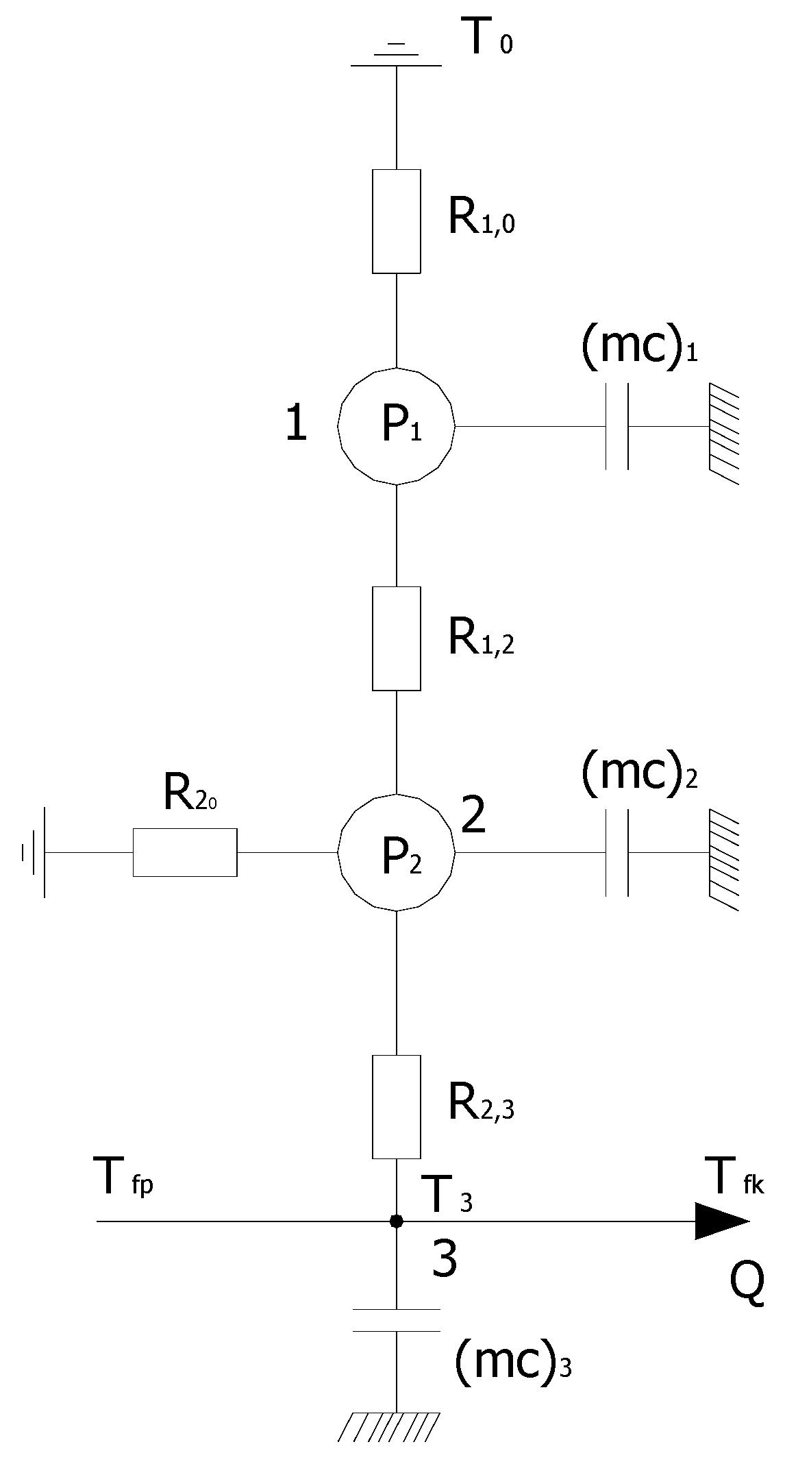
The second method used in the determination of the static and dynamic properties of the collector will be the ETN method developed by Chochowski [44]. The flat-plate solar collector was presented in the form of a two-terminal-pair network, and three homogeneous bodies were identified in the collector structure: the transparent cover, the absorber and the working medium presented as active nodes (Figure 1). The method allows an analysis of both the steady and transient states of the collector. In addition, it is possible to simulate the operation of collector batteries that may be interconnected serially or in parallel. Using this method, a heat steam is the equivalent of electrical current, thermal resistances–resistors and temperature distribution–voltage reduction.

Node No. 1, in which energy is emitted in half of the thickness with a power of P1 absorbing part of the solar radiation falling on the plane, corresponds to the glass cover (average temperature of T1).

Node No. 2, in which, as a result of absorbing solar rays passing through the glass cover, thermal energy with a power of P2 is emitted on the surface, represents the absorber (average temperature of T2).

Node No. 3 represents the working medium flowing through the solar collector with average temperature of T3 determined from:

$${\mathrm{T}}_3=\frac{1}{2}\left({\mathrm{T}}_{\mathrm{fi}}+{\mathrm{T}}_{\mathrm{fo}}\right)$$

(5)

Thermal streams P flow between the network nodes and the loss center (environment) with thermal resistance R. Thermal resistances present in the diagram (Figure 1) have the following physical sense:

• R_1,0—thermal resistance between the front cover and the environment [K/W]
• R_1,2—thermal resistance between the front cover and the absorber [K/W]
• R_2,0—thermal resistance between the absorber and the environment, calculated towards the bottom of the collector [K/W]
• R_2,3—thermal resistance between the absorber and the working medium [K/W]
• (mc)₁—thermal capacity of the glass cover [J/K]
• (mc)₂—thermal capacity of the absorber [J/K]
• (mc)₃—thermal capacity of the working medium [J/K]

The presented thermal network was solved in the form of a system of differential equations combining heat capacity values of specific homogeneous bodies and heat resistance between the particular components of the collector Equation (6).

$${\left(\mathrm{mc}\right)}_{\mathrm{i}}\frac{{\mathrm{dT}}_{\mathrm{i}}}{\mathrm{dt}}+{\mathrm{T}}_{\mathrm{i}}{\displaystyle \sum }_{\mathrm{j}=1}^{\mathrm{n}+1}{\mathsf{\Lambda }}_{\mathrm{ij}}-{\displaystyle \sum }_{\mathrm{j}=1}^{\mathrm{n}+1}{\mathsf{\Lambda }}_{\mathrm{ij}}{\mathrm{T}}_{\mathrm{j}}={\mathrm{P}}_{\mathrm{i}}+{\mathsf{\Lambda }}_{\mathrm{i}0}{\mathrm{T}}_0$$

(6)

The solution of Equation (6) follows the solving system of linear equations, which takes on the matrix form of Equation (7), where the matrix c Equation (8) is a diagonal matrix of thermal capacities of particular components and the matrix Λ Equation (9) is a matrix of thermal conductivities of particular network nodes.

$$\mathrm{c}\frac{\mathrm{d} \overline{\mathrm{T}}\left(\mathrm{t}\right)}{\mathrm{dt}}+\mathsf{\Lambda } \overline{\mathrm{T}}\left(\mathrm{t}\right)= \overline{\mathrm{P}}\left(\mathrm{t}\right)$$

(7)

where:

$$\mathrm{c}=\begin{array}{ccc}{\left(\mathrm{mc}\right)}_1& 0& 0\\ 0& {\left(\mathrm{mc}\right)}_2& 0\\ 0& 0& {\left(\mathrm{mc}\right)}_3\end{array}$$

(8)

$$\mathsf{\Lambda }=\left[\begin{array}{ccc}{\mathsf{\Lambda }}_{11}& {\mathsf{\Lambda }}_{12}& {\mathsf{\Lambda }}_{13}\\ {\mathsf{\Lambda }}_{21}& {\mathsf{\Lambda }}_{22}& {\mathsf{\Lambda }}_{23}\\ {\mathsf{\Lambda }}_{31}& {\mathsf{\Lambda }}_{32}& {\mathsf{\Lambda }}_{33}\end{array}\right]$$

(9)

By both sides multiplying by the inverse matrix c⁻¹, Equation (6) takes the following form Equation (10):

$$\frac{\mathrm{d} \overline{\mathrm{T}}\left(\mathrm{t}\right)}{\mathrm{dt}}=-\left({\mathrm{c}}^{-1}\times \mathsf{\Lambda }\right)\times \overline{\mathrm{T}}+{\mathrm{c}}^{-1}\times \overline{\mathrm{P}}$$

(10)

The matrix notation Equation (11) obtains as result of substituting matrices Equations (8) and (9) to matrix Equation (10) and can be after transformed into the form of Equation (12).

$$\frac{\mathrm{d}}{\mathrm{dt}}\left[\begin{array}{c}{\mathrm{T}}_1\\ {\mathrm{T}}_2\\ {\mathrm{T}}_3\end{array}\right]=\left[\begin{array}{ccc}{\mathrm{mc}}_1& 0& 0\\ 0& {\mathrm{mc}}_2& 0\\ 0& 0& {\mathrm{mc}}_3\end{array}\right]\times \left[\begin{array}{ccc}{\mathsf{\Lambda }}_{11}& {\mathsf{\Lambda }}_{12}& {\mathsf{\Lambda }}_{13}\\ {\mathsf{\Lambda }}_{21}& {\mathsf{\Lambda }}_{22}& {\mathsf{\Lambda }}_{23}\\ {\mathsf{\Lambda }}_{31}& {\mathsf{\Lambda }}_{32}& {\mathsf{\Lambda }}_{33}\end{array}\right]\times \left[\begin{array}{c}{T}_1\\ T_2\\ T_3\end{array}\right]+\left[\begin{array}{ccc}{\mathrm{mc}}_1& 0& 0\\ 0& {\mathrm{mc}}_2& 0\\ 0& 0& {\mathrm{mc}}_3\end{array}\right]\times \left[\begin{array}{c}{\mathrm{P}}_1\\ {\mathrm{P}}_2\\ {\mathrm{P}}_3\end{array}\right]$$

(11)

$$\frac{\mathrm{d}}{\mathrm{d}\mathrm{t}}\left[\begin{array}{c}{\mathrm{T}}_1\\ {\mathrm{T}}_2\\ {\mathrm{T}}_3\end{array}\right]=\left[\begin{array}{ccc}\frac{1}{{\mathrm{m}\mathrm{c}}_1}& 0& 0\\ 0& \frac{1}{{\mathrm{m}\mathrm{c}}_2}& 0\\ 0& 0& \frac{1}{{\mathrm{m}\mathrm{c}}_3}\end{array}\right]\times \left[\begin{array}{ccc}{\mathsf{\Lambda }}_{11}& {\mathsf{\Lambda }}_{12}& {\mathsf{\Lambda }}_{13}\\ {\mathsf{\Lambda }}_{21}& {\mathsf{\Lambda }}_{22}& {\mathsf{\Lambda }}_{23}\\ {\mathsf{\Lambda }}_{31}& {\mathsf{\Lambda }}_{32}& {\mathsf{\Lambda }}_{33}\end{array}\right]\times \left[\begin{array}{c}{\mathrm{T}}_1\\ {\mathrm{T}}_2\\ {\mathrm{T}}_3\end{array}\right]+\left[\begin{array}{ccc}\frac{1}{{\mathrm{m}\mathrm{c}}_1}& 0& 0\\ 0& \frac{1}{{\mathrm{m}\mathrm{c}}_2}& 0\\ 0& 0& \frac{1}{{\mathrm{m}\mathrm{c}}_3}\end{array}\right]\times \left[\begin{array}{c}{\mathrm{P}}_1\\ {\mathrm{P}}_2\\ {\mathrm{P}}_3\end{array}\right]$$

(12)

The matrix of the system and a matrix of the input Equation (13) is the solution to the matrix of state variables.

$$\frac{\mathrm{d}}{\mathrm{d}\mathrm{t}}\left[\begin{array}{c}{\mathrm{T}}_1\\ {\mathrm{T}}_2\\ {\mathrm{T}}_3\end{array}\right]=\left[\begin{array}{c}\frac{{\mathsf{\Lambda }}_{11}}{{\mathrm{m}\mathrm{c}}_1} \frac{{\mathsf{\Lambda }}_{12}}{{\mathrm{m}\mathrm{c}}_1} \frac{{\mathsf{\Lambda }}_{13}}{{\mathrm{m}\mathrm{c}}_1}\\ \frac{{\mathsf{\Lambda }}_{21}}{{\mathrm{m}\mathrm{c}}_2} \frac{{\mathsf{\Lambda }}_{22}}{{\mathrm{m}\mathrm{c}}_2} \frac{{\mathsf{\Lambda }}_{23}}{{\mathrm{m}\mathrm{c}}_2}\\ \frac{{\mathsf{\Lambda }}_{31}}{{\mathrm{m}\mathrm{c}}_3} \frac{{\mathsf{\Lambda }}_{32}}{{\mathrm{m}\mathrm{c}}_3} \frac{{\mathsf{\Lambda }}_{33}}{{\mathrm{m}\mathrm{c}}_3}\end{array}\right]\times \left[\begin{array}{c}{\mathrm{T}}_1(\mathrm{t})\\ {\mathrm{T}}_2(\mathrm{t})\\ {\mathrm{T}}_3(\mathrm{t})\end{array}\right]+\left[\begin{array}{c}\frac{{\mathrm{P}}_1}{{\mathrm{m}\mathrm{c}}_1}\\ \frac{{\mathrm{P}}_2}{{\mathrm{m}\mathrm{c}}_2}\\ \frac{{\mathrm{P}}_3}{{\mathrm{m}\mathrm{c}}_3}\end{array}\right]\times \mathrm{u}(\mathrm{t})$$

(13)

The matrix of the system expresses the ratio of thermal conductivity of network nodes to their thermal capacity. The individual homogeneous bodies temperatures of a solar collector are variables of the condition, while the input column matrix is the ratio of the heat output of a node to its thermal capacity. The presented method allows not only an analysis of transient states of the temperature values of a particular component, but also the heat flow distribution between them. In addition, it is possible to simulate the operation of collector batteries that may be interconnected serially or in parallel. The document also provides an accurate algorithm enabling calculation of particular coefficient values of the differential equation.

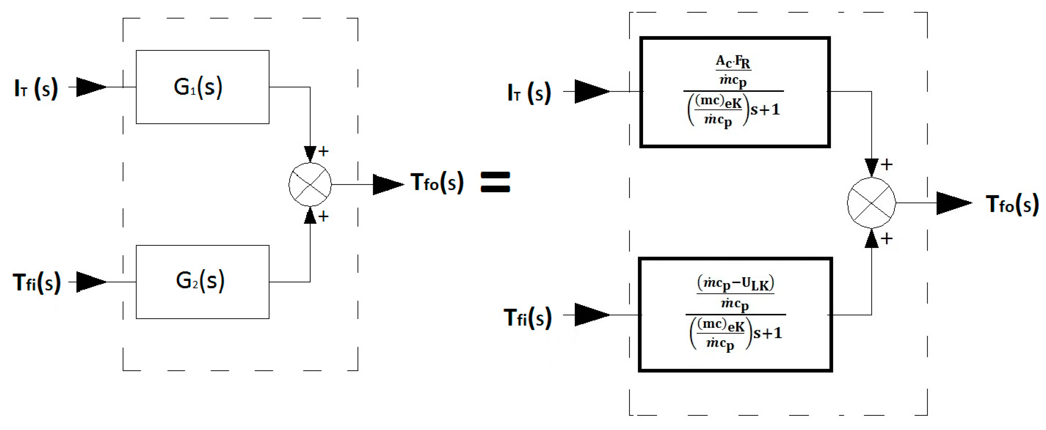
The third method used in the determination of the static and dynamic properties of the collector will be one based on parametric identification developed by Obstawski [61]. The diagnostics method for a solar heating system allows the determination of static properties under operating conditions, i.e., the heat loss coefficient U_L, the collector efficiency coefficient F’, the heat removal factor F_R, and heat capacity values j (mc)_e, as well as dynamic properties: gain kp, the time constant T_c of the collector. The calculation method is based on two equivalent models: one based on a database using parametric analysis methods, and the other based on an energy balance combining the characteristic parameters of a collector (modification of the HWB equation). The model in the form of a differential Equation (12), obtained as a result of parametric identification, is converted by using discrete Laplace transform into discrete operator transmittance Equation (14), and then, by means of relation Equation (16), into continuous transmittance. Likewise, the analytical model Equation (13) can be converted into equivalent operator transmittance Equation (17) by using the Laplace transform Equation (15). Comparison of models adequately Equations (14)–(19) makes it possible to determine the characteristic parameters of the diagnosed system (Figure 2). The diagnostics method for a solar collector system enables the determination of its static and dynamic properties based on operating data, which makes it versatile.

$$\mathrm{A}\left(\mathrm{z}\right)\mathrm{y}\left(\mathrm{t}\right) = \mathrm{B}\left(\mathrm{z}\right)\mathrm{u}\left(\mathrm{t}-{\mathrm{n}}_{\mathrm{k}}\right)+\mathrm{e}\left(\mathrm{t}\right)$$

(14)

$$\frac{{\mathrm{dT}}_{\mathrm{out}}\left(\mathrm{t}\right)}{\mathrm{dt}}=\frac{\mathrm{I}\left(\mathrm{t}\right)\times {\mathrm{A}}_{\mathrm{C}}\times {\mathrm{F}}_{\mathrm{R}}-{ \dot{\mathrm{m}} \mathrm{c}}_{\mathrm{p}}\times \left({\mathrm{T}}_{\mathrm{out}}\left(\mathrm{t}\right)-{\mathrm{T}}_{\mathrm{in}}\left(\mathrm{t}\right)\right)-{\mathrm{U}}_{\mathrm{LK}}\times \left({\mathrm{T}}_{\mathrm{in}}\left(\mathrm{t}\right)-{\mathrm{T}}_{\mathrm{amb}}\left(\mathrm{t}\right)\right)}{{\left(\mathrm{mc}\right)}_{\mathrm{eK}}}$$

(15)

$$\mathrm{G}\left(\mathrm{s}\right)=\frac{{\mathrm{kp}}_1}{{\mathrm{T}}_{\mathrm{C}1}\mathrm{s}+1}\times \frac{{\mathrm{kp}}_2}{{\mathrm{T}}_{\mathrm{C}2}\mathrm{s}+1}\times \dots \times \frac{{\mathrm{kp}}_{\mathrm{n}}}{{\mathrm{T}}_{\mathrm{Cn}}\mathrm{s}+1}$$

(16)

$${\mathrm{T}}_{\mathrm{out}}\left(\mathrm{s}\right)=\frac{\frac{{\mathrm{A}}_{\mathrm{c}}·{\mathrm{F}}_{\mathrm{R}}}{{ \dot{\mathrm{m}} \mathrm{c}}_{\mathrm{p}}}}{\left(\frac{{\left(\mathrm{mc}\right)}_{\mathrm{eK}}}{{ \dot{\mathrm{m}} \mathrm{c}}_{\mathrm{p}}}\right)\mathrm{s}+1}\times \mathrm{I}\left(\mathrm{s}\right)+\frac{\frac{\left({ \dot{\mathrm{m}} \mathrm{c}}_{\mathrm{p}}-{\mathrm{U}}_{\mathrm{LK}}\right)}{{ \dot{\mathrm{m}} \mathrm{c}}_{\mathrm{p}}}}{\left(\frac{{\left(\mathrm{mc}\right)}_{\mathrm{eK}}}{{ \dot{\mathrm{m}} \mathrm{c}}_{\mathrm{p}}}\right)\mathrm{s}+1}\times {\mathrm{T}}_{\mathrm{in}}\left(\mathrm{s}\right)+\frac{\frac{{\mathrm{U}}_{\mathrm{LK}}}{{ \dot{\mathrm{m}} \mathrm{c}}_{\mathrm{p}}}}{\left(\frac{{\left(\mathrm{mc}\right)}_{\mathrm{eK}}}{{ \dot{\mathrm{m}} \mathrm{c}}_{\mathrm{p}}}\right)\mathrm{s}+1}\times {\mathrm{T}}_{\mathrm{amb}}\left(\mathrm{s}\right)$$

(17)

$${\mathrm{T}}_{\mathrm{out}}\left(\mathrm{s}\right)=\frac{{\mathrm{kp}}_1}{{\mathrm{T}}_{\mathrm{C}}\left(\mathrm{s}\right)+1}\times \mathrm{I}\left(\mathrm{s}\right)+\frac{{\mathrm{kp}}_2}{{\mathrm{T}}_{\mathrm{C}}\left(\mathrm{s}\right)+1}\times {\mathrm{T}}_{\mathrm{in}}\left(\mathrm{s}\right)$$

(18)

$${\mathrm{T}}_{\mathrm{out}}\left(\mathrm{s}\right)=\frac{\frac{{\mathrm{A}}_{\mathrm{c}}·{\mathrm{F}}_{\mathrm{R}}}{{ \dot{\mathrm{m}} \mathrm{c}}_{\mathrm{p}}}}{\left(\frac{{\left(\mathrm{mc}\right)}_{\mathrm{eK}}}{{ \dot{\mathrm{m}} \mathrm{c}}_{\mathrm{p}}}\right)\mathrm{s}+1}\times \mathrm{I}\left(\mathrm{s}\right)+\frac{\frac{\left({ \dot{\mathrm{m}} \mathrm{c}}_{\mathrm{p}}-{\mathrm{U}}_{\mathrm{LK}}\right)}{{ \dot{\mathrm{m}} \mathrm{c}}_{\mathrm{p}}}}{\left(\frac{{\left(\mathrm{mc}\right)}_{\mathrm{eK}}}{{ \dot{\mathrm{m}} \mathrm{c}}_{\mathrm{p}}}\right)\mathrm{s}+1}\times {\mathrm{T}}_{\mathrm{in}}\left(\mathrm{s}\right)$$

(19)

The only requirement is the maintenance of constant medium flow rate in the system during the experiment. Thus, it is possible to determine the static and dynamic properties of the collector under operating conditions, and to specify the impact of solar irradiance variation and collector heat load on its properties.

4. Comparison of Characteristic Parameter Values Determined for a Collector Using Different Methods

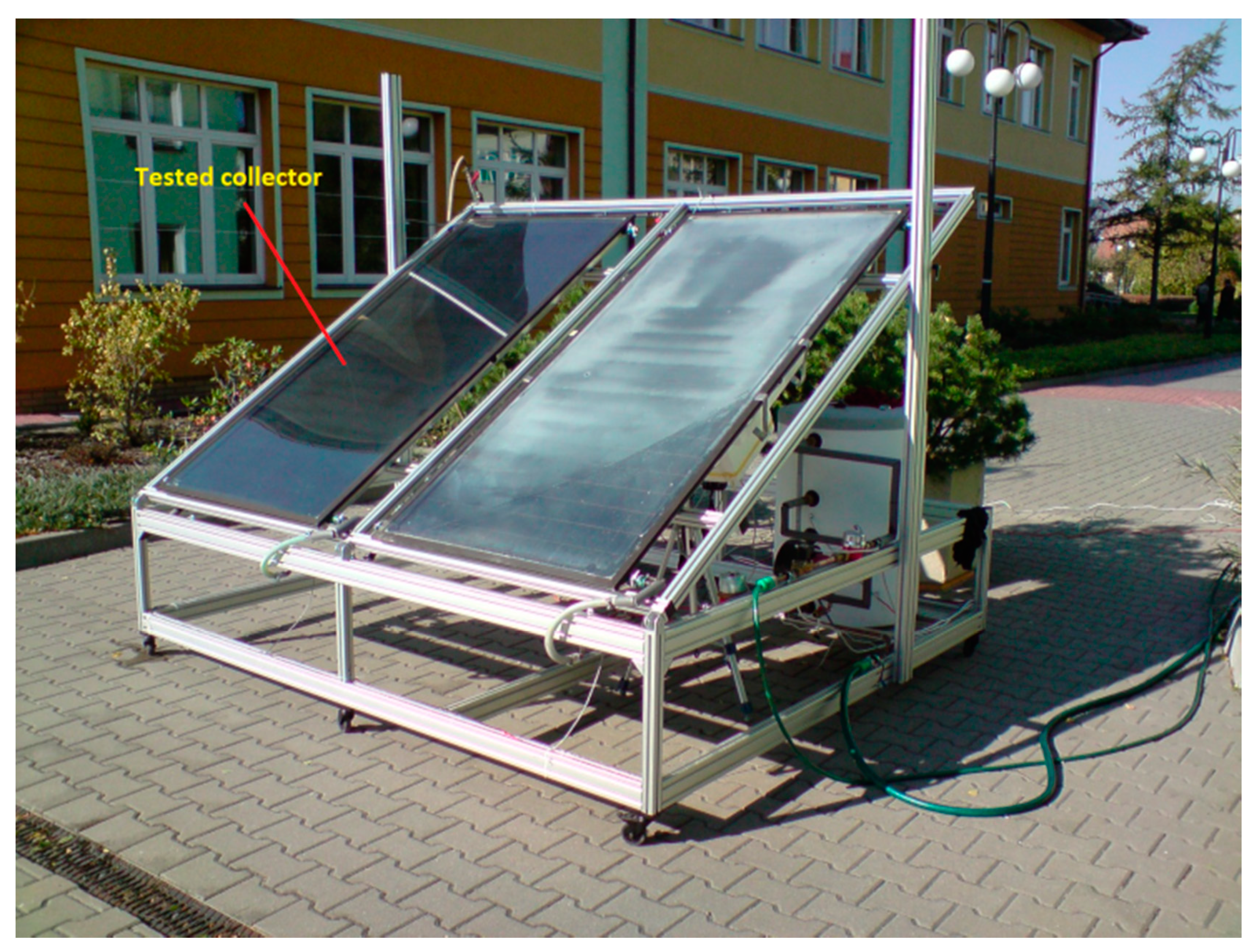
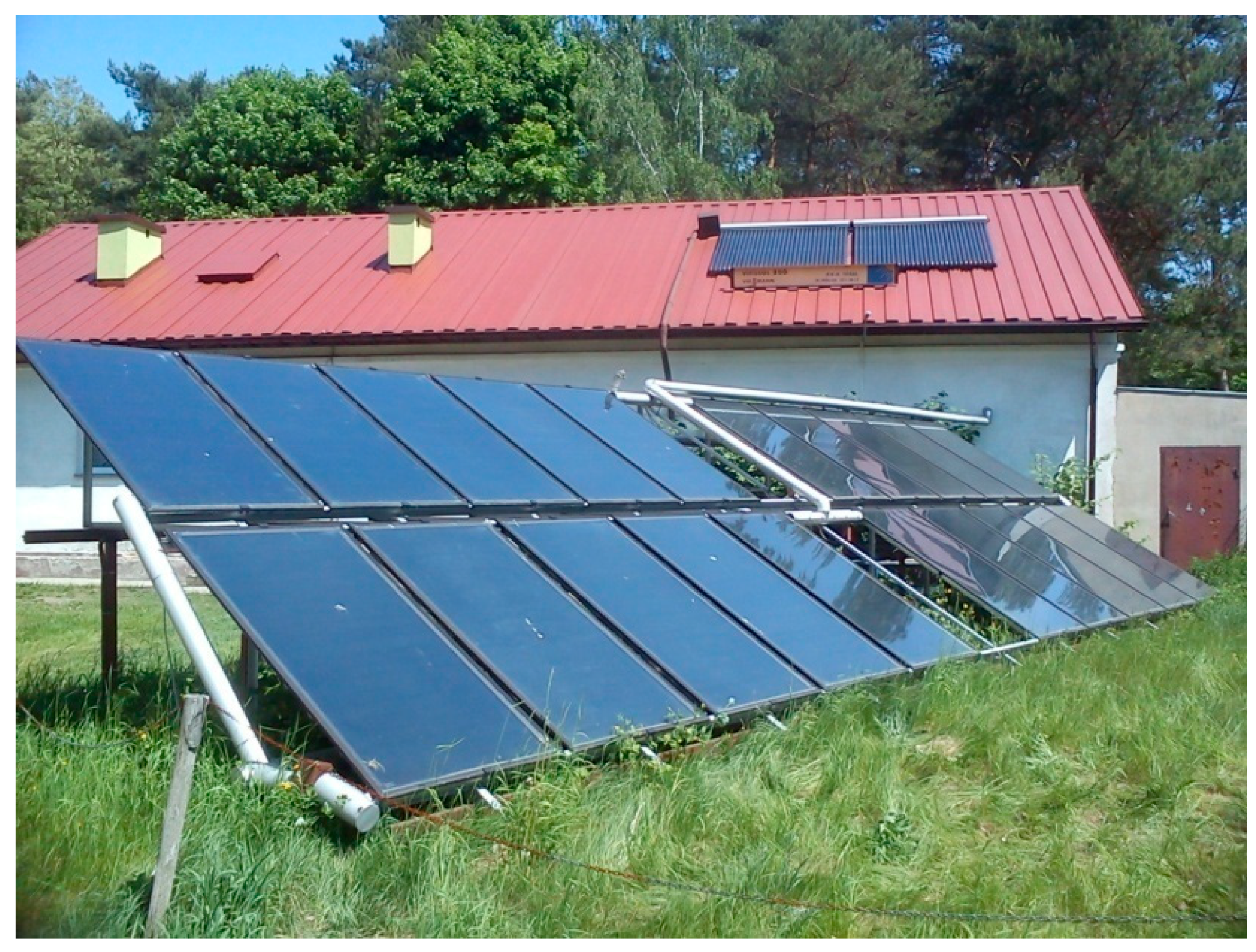
A flat-plate solar collector is a non-fixed object operating in transient states [41]. In consequence, both the static and dynamic properties of the flat-plate solar collector are variable and depend on operating conditions and heat load [61]. In hybrid energy installations, cooperation between segments of the system has the most significant impact on the behavior of the solar collector. Thus, when designing the control system of a solar heating installation, it is very important to know how and within what limits the values of the characteristic parameters of the collector that describe its static and dynamic properties change, starting from the design process, through standard tests under indoor and outdoor conditions compliant with the ISO 9806:2017 standard [20], and heat load with a hot water storage tank under operating conditions. Making a mistake in the design process for controlling a solar installation in a hybrid energy system will decrease efficiency of the solar segment and can cause instability of the solar segment under certain operating conditions. The presented groups of methods allow an analysis of the variability of characteristic parameter values. An example of an analysis will be presented for a flat-plate collector whose static properties, represented by efficiency characteristics, as well as dynamic properties—the time constant substitute—were determined under indoor conditions in accordance with the ISO 9806:2017 [20] standard (

Table 2. Characteristic parameters of the tested collector according to iso 9806 indoor conditions.

Normal Characteristic	Effective Heat Capacity [kJ/m2K]	Time Constant Substitute [s]	Collector Area [m2]	Aperture Area [m2]	Weight [kg]	Absorber Material	Glass Thickness [mm]	Insulation Thickness [mm]	Maximum Pressure [bar]	Volume [l]
η = 0.79 − 4.17Tm − 0.01Tm2	6.73	80	2.0	1.76	43	Aluminum	4.0	Basalt 40	6	1.3

), and will be regarded as model. Therefore, the particular tests were performed in accordance with the standard for a volume flow of the working medium amounting to 0.02 dm³/min per square meter of the tested collector aperture. The presented analyses of efficiency characteristics and step response enable the time constant substitute and the effective heat capacity of the tested collector to be determined using measurement data from two test stands. The first stand allows the determination of efficiency characteristics and time constant substitute of the collector under outdoor conditions in accordance with the ISO 9806:2017 [20] standard, and enables performance testing of heat loaded with a 100 dm³ storage tank with one or two collectors connected in parallel (Figure 3). The operating modes of the installation can be changed by setting the position of electro valves. The measurement of fluid temperature and ambient temperature is performed by PT1000 sensors in a four-transverse system.

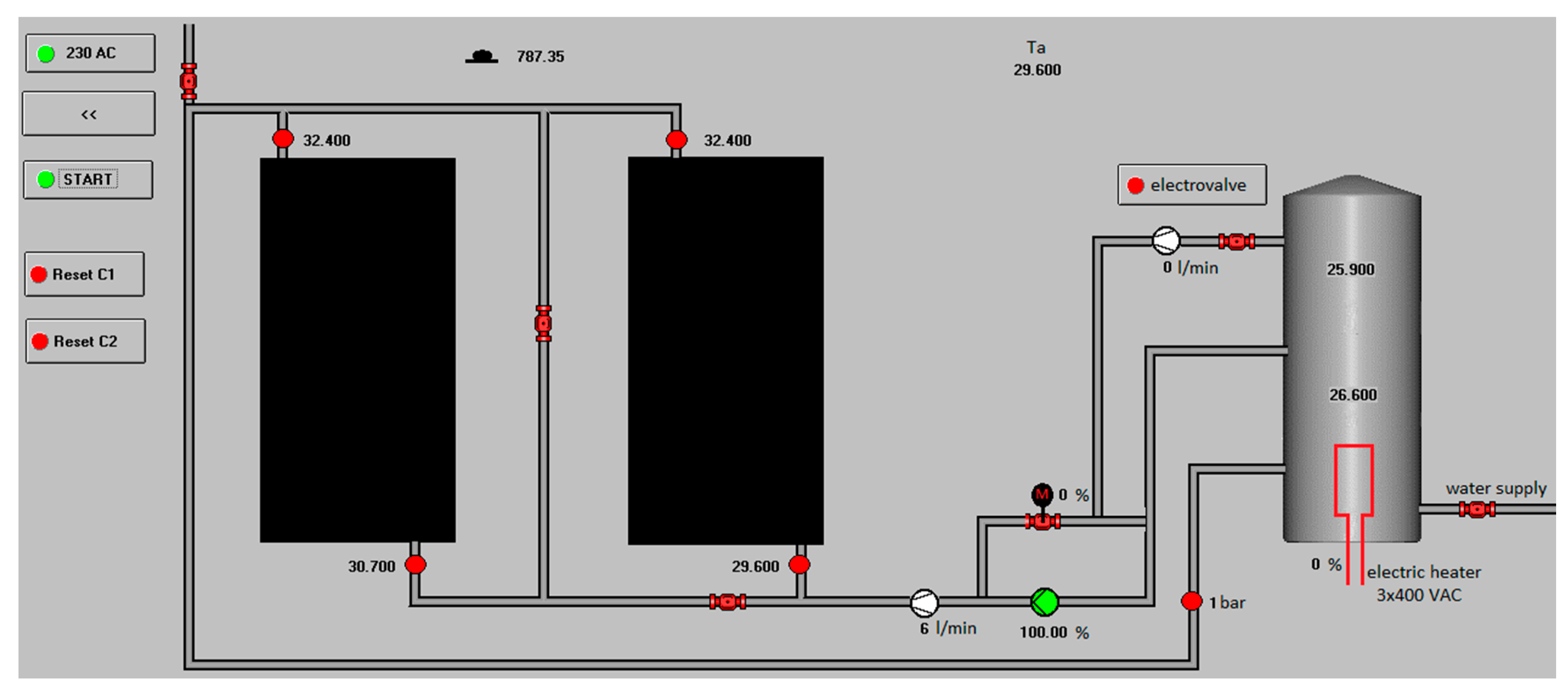
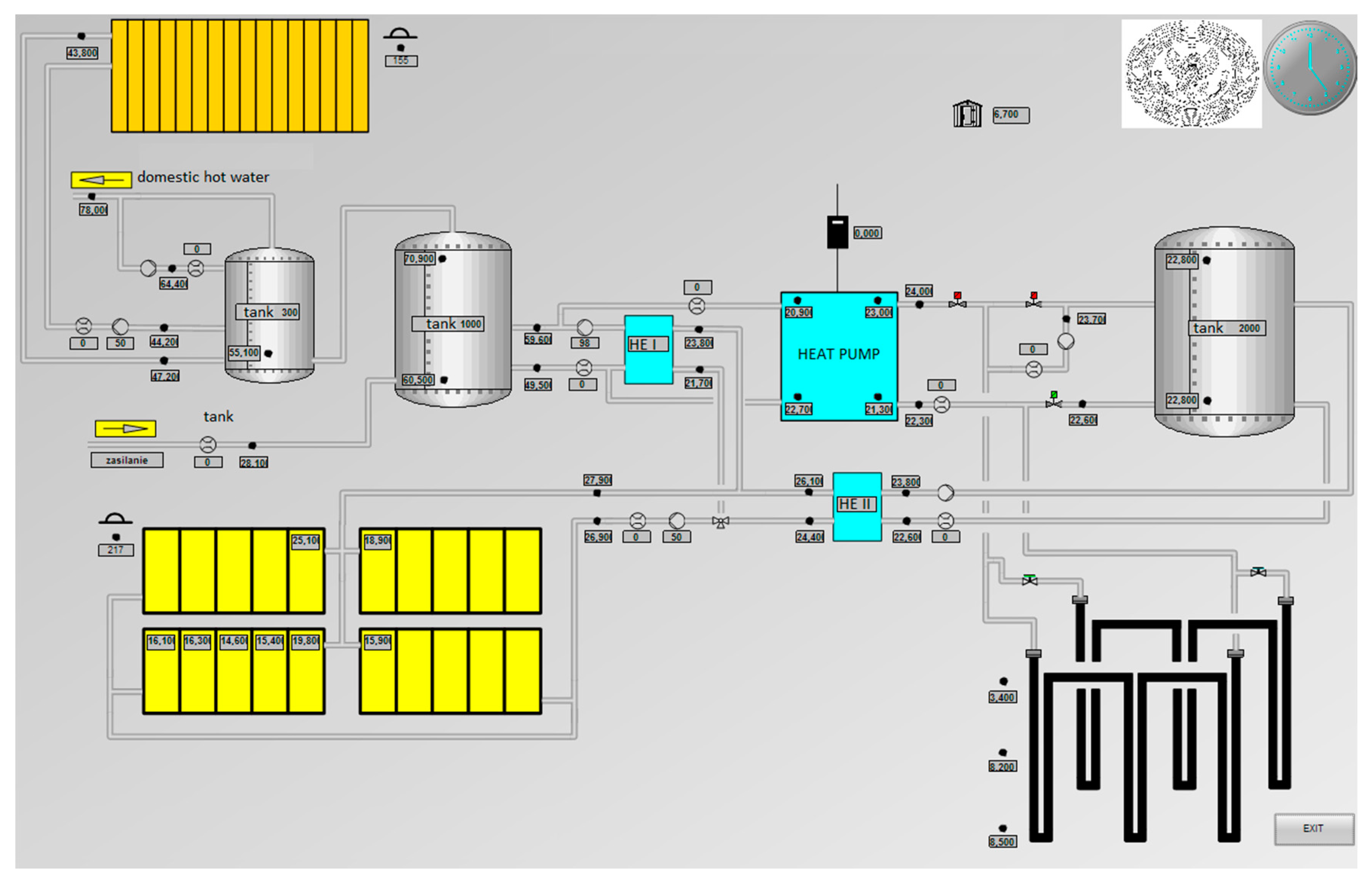
The sensors are made with class A accuracy. Sensors that measure fluid temperature are located in special capillaries soldered inside the pipes. Flow rate is measured by a turbine flow meter working in a current loop. Solar irradiance is measured by a class 1pyranometer. Fluid pressure is measured by a sensor with a 0–10 bar range and a 0–10 VDC voltage output. The hydraulic installation uses a circulation pump with the ability to continuously adjust flow rate, using a 0–10 VDC external voltage signal. All measurement components are integrated into one measurement system based on a Programmable Logic Controller (PLC), where the control algorithm of installation operation has been implemented. The PLC is connected using an Ethernet protocol to the Supervisory Control and Data Acquisition (SCADA) system with visualization and measured data acquisition (Figure 4). The measured physical values are recorded with a sampling period of 1 s.

The second test stand is a hybrid energy system based on the cooperation of two solar heating installations (flat and vacuum solar collectors) and a ground heat pump with a capacity of about 10.5 kW (Figure 5) [7]. The solar heating installation based on flat solar collectors is composed of four sections connected in parallel, consisting of five collectors each. The total area of aperture of the flat-plate collectors is 40 m². This section of the hybrid system is thermally loaded with a buffer tank about 1000 L in volume. A buffer tank about 300 L in volume provides thermal load for vacuum solar collectors with an aperture area of 6 m². The priority function of heating domestic hot water in this system is served by a ground heat pump. The nominal minimum temperature of domestic hot water in the buffer tank is 40 °C and it is the initial operating temperature value for flat and vacuum collectors. The lower priority source of energy for the heat pump involves a ground heat exchanger. An alternative source of energy includes a buffer tank about 2000 L in volume, which is connected to the flat-plate collector via a plate heat exchanger. Such a hydraulic construction of the hybrid installation makes it possible to accumulate energy surplus from the flat-plate collectors in the buffer tank and protect the solar installation against preheating. The energy accumulated in this buffer tank is used to regenerate the ground heat exchanger. The PT1000 class A temperature sensor in a four-transverse system has been located in a measurement capillary soldered inside the pipes. The flow rate in every segment of the system is measured by pulse flow meters with a resolution of 1 impulse per 1 L. An external voltage signal within a range of 0–10 VDC makes it possible to change the flow rate. Solar irradiance is measured by a class 1 pyranometer. The visualization of the system control unit and the acquisition of the measured data of test stand II (Figure 6) are similar to test stand I described above.

4.1. Analysis of Static and Dynamic Properties According to ISO 9806 under Outdoor Conditions

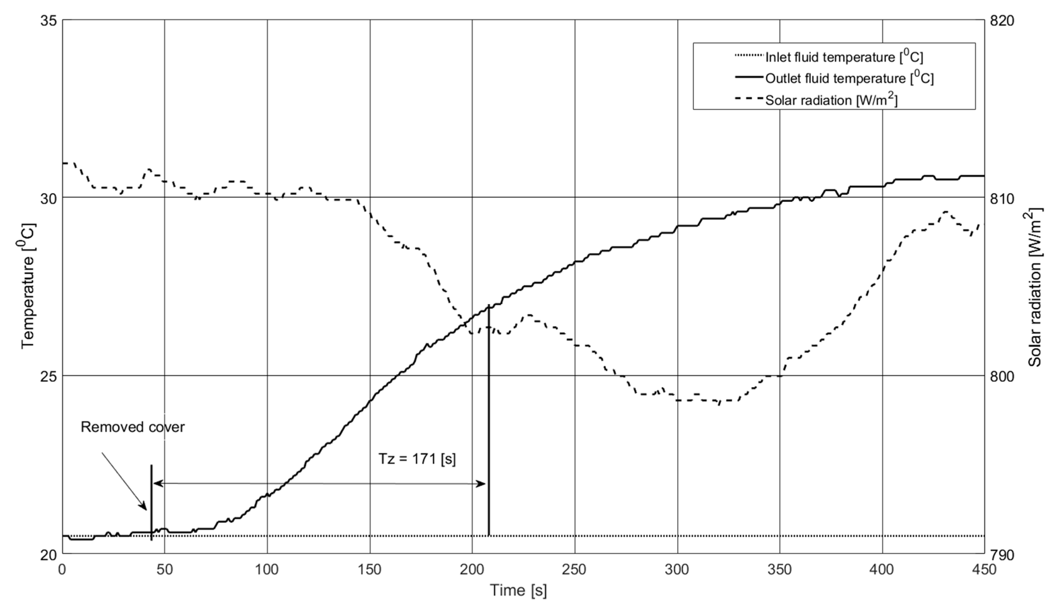
Figure 7 presents the step response of the tested collector determined based on an experiment performed according to ISO 9806:2017 [20] outdoor conditions in test stand I. The characteristics were determined for an inlet temperature of the working medium of 20.5 °C, an ambient temperature of 20 °C, solar irradiance of 806 W/m² ± 6 W/m² and a flow rate of 2.16 dm³/min, as per the standard. In accordance with the methodology described in the ISO 9806:2017 standard [20], a time constant substitute of 171 s was read from the step response.

Using relation Equation (20) [57], effective heat capacity of 14.3 kJ/m²K was calculated. Figure 8 shows the efficiency characteristics of the tested collector developed based on data measured under outdoor conditions in test stand I.

$${\left(\mathrm{mc}\right)}_{\mathrm{e}}=\frac{ \dot{\mathrm{m}}\times {\mathrm{c}}_{\mathrm{p}}\times {\mathrm{T}}_{\mathrm{z}}}{{\mathrm{A}}_{\mathrm{p}}}$$

(20)

Efficiency characteristics were determined described using relation Equation (21) using the method of least squares. When analyzing the characteristics, it should be noticed that the collector zero-loss efficiency is slightly lower than the efficiency determined under indoor conditions and amounts to 77%, whereas the coefficient of temperature-dependent heat losses is significantly higher and amounts to 54.8 W/m²K² (Table 2).

η = 0.77 − 4.92 T_m − 54.8T_m²

(21)

Using relations Equations (2) and (4), the values of F’ and U_L were calculated in relation to ambient temperature (Table 2). The value of F_R was calculated using relation Equation (22).

$${\mathrm{F}}_{\mathrm{R}}=\frac{{ \dot{\mathrm{m}} \mathrm{c}}_{\mathrm{p}}}{{\mathrm{A}}_{\mathrm{p}}{\mathrm{U}}_{\mathrm{L}}}\left[1-\exp \left(-\frac{{\mathrm{A}}_{\mathrm{p}}{\mathrm{U}}_{\mathrm{L}}{\mathrm{F}}^{\prime }}{{ \dot{\mathrm{m}} \mathrm{c}}_{\mathrm{p}}}\right)\right]$$

(22)

4.2. Analysis of Static and Dynamic Properties Using the Equivalent Thermal Network (ETN)

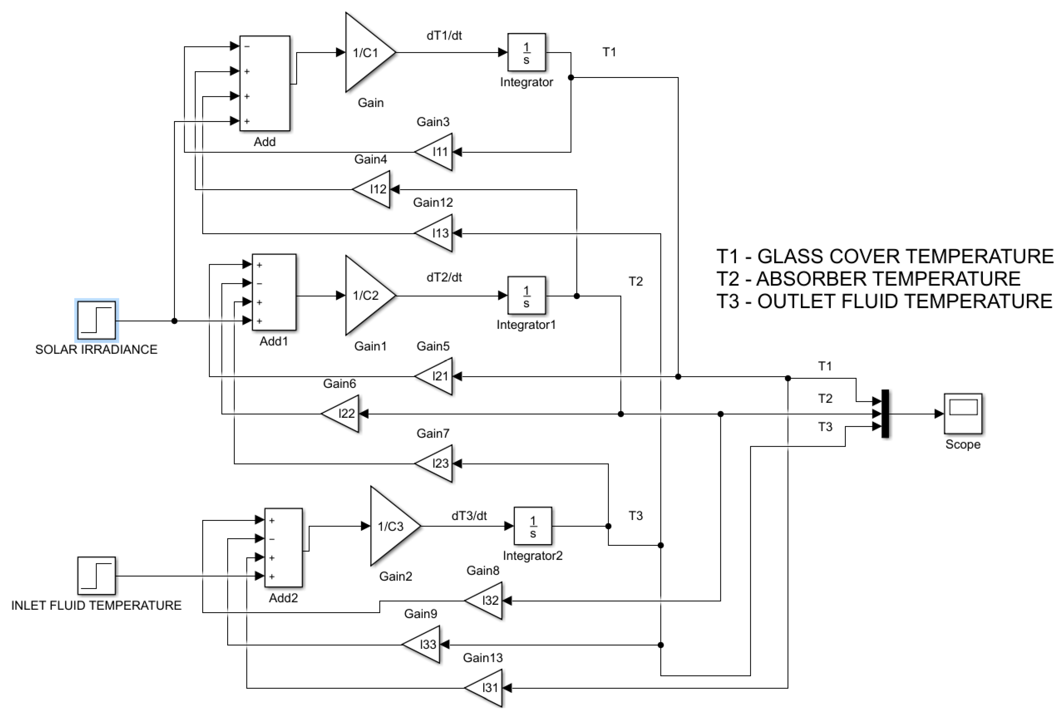
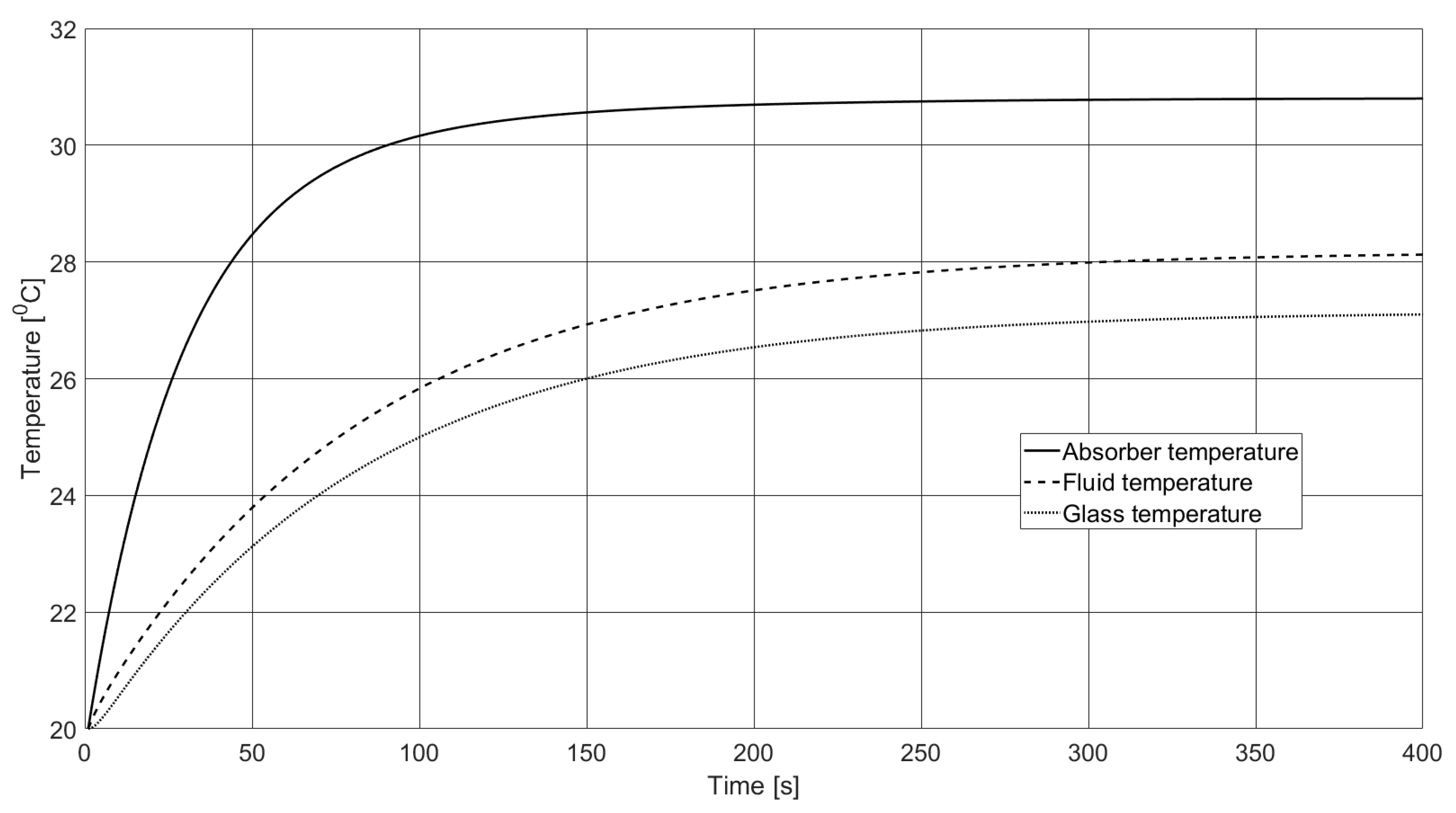
The ETN method developed by Chochowski [44] was used to analyze the static and dynamic properties of the tested solar collector during the design process. The specific values of heat resistance were calculated based on the collector material data. The thermal network was implemented in Simulink (Figure 9). The simulation was performed in accordance with the standard for a flow rate of 2.16 dm³/min. Figure 10 shows the step response of the tested collector, prepared for a solar irradiance value of 1000 W/m² and a working medium inlet temperature of 20 °C. In contrast to other methods, the ETN method allows an analysis of the impact of structural parameters on the energy flow and temperature distribution between specific homogeneous bodies of the collector. Therefore, it was possible to develop a step response for the glass cover, the absorber and the working medium.

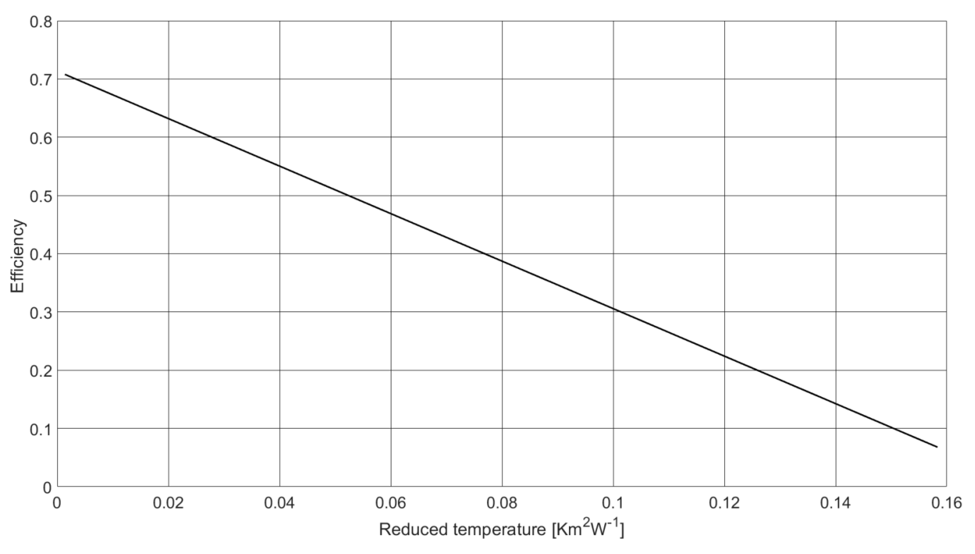
When analyzing the step response family (Figure 10), it should be noticed that the absorber is characterized by the shortest time constant of 30 s, and the transparent glass cover is characterized by the longest time constant of 86 s. The working medium time constant is 77 s. When comparing efficiency characteristics determined using the thermal network method (Figure 11) and efficiency characteristics determined according to the standard under indoor and outdoor conditions, attention should be paid to the significantly reduced zero-loss efficiency value of 0.71 and the significantly reduced coefficient of temperature-dependent heat losses of 0.0001 W/m²K² (Table 2). This coefficient value probably results from the linear character of the collector model. Using relations Equations (2), (4) and (22), the values of F’, F_R and U_L were calculated in relation to ambient temperature (Table 2).

η = 0.71 − 4.07T_m − 0.0001T_m²

(23)

4.3. Analysis of Static and Dynamic Properties of the Collector Using the Parametric Identification Method for Heat Load with a Hot Water Storage Tank

As already mentioned, the solar collector is a non-fixed object, whose characteristic parameters depend on the operating conditions. The determination of characteristic parameters under operating conditions is possible with the use of the method developed by Obstawski et al. [59] classified into the third group of methods, based on parametric identification. The method allows the determination of the static and dynamic properties of the collector based on the recorded time series of working medium temperature and solar irradiance. It is thus possible to compare the characteristic parameters of the collector assumed at the design stage to those determined during standard tests and under operating conditions. The analysis will be presented based on an example of the operation of two solar systems:

(a)

two collectors loaded with a 100 dm³ storage tank (test stand I)

(b)

a battery of 20 collectors with a total absorber area of 40 m², loaded with a 1000 dm³ storage tank (test stand II).

In the case of system I, the volume flow of the medium through a single collector is compliant with the ISO 9806 standard and amounts to 0.02 kg/m² per the absorber area. In the case of system II, the experiment was performed for a flow rate 50% lower than the standard value. The applied method enables the determination of collector parameters for pre-flow in accordance with the normative method.

4.3.1. Collector Parameters Determined for a 100 dm³ Load (Test Stand I)

Figure 12 shows the values of solar irradiance and temperature of the medium during the experiment. It should be noticed that at the beginning of the experiment, variable weather conditions prevailed. Solar irradiance was within a range of 400–950 W/m². After 6000 s, solar conditions stabilized and the solar irradiance value reached 950 W/m². In the last phase of the test, variable weather conditions appeared again. For a constant volume flow rate of the working medium in the system, amounting to 4.0 dm³/min, the working medium temperature increased from 30 to 78 °C. Based on the recorded measurement data using the parametric identification method, a model was created in the form of differential Equation (24), which was verified and then transformed, using Tustin’s method, into a continuous one, and was approximated to an operator transform form described by the general Equation (25).

A(z) = 1 − 0.857z⁻¹− 0.09157z⁻² − 0.04576z⁻³
B₁(z) = 5.341e⁻⁵z⁻¹
B₂(z) = 0.0053889z⁻¹

(24)

$${\mathrm{T}}_{\mathrm{fo}}\left(\mathrm{s}\right)=\frac{0.0094}{207.9\mathrm{s}+1}\times {\mathrm{I}}_{\mathrm{T}}\left(\mathrm{s}\right)+\frac{0.949}{207.9\mathrm{s}+1}\times {\mathrm{T}}_{\mathrm{fi}}\left(\mathrm{s}\right)$$

(25)

Having the gain coefficient kp₁ = 0.0094 and kp₂ = 0.949 for the initial temperature of the medium within a system operation range of 30–75 °C and solar irradiance of 970 W/m², the efficiency characteristics (Figure 13) was determined as described by Equation (26). Attention should be paid to the significantly reduced value of the zero-loss efficiency coefficient and the heat loss coefficient (Table 2). Figure 14 presents the step response of the tested collector. The heat loaded collector is characterized by a significantly higher time constant of 207.9 s, which means that the solar collector heat capacity under the load will be significantly higher than in a state with no load. The values of characteristic parameters are determined using relation Equation (19) and the model presented in Table 1 (item 30).

η = 0.68 − 4.8T_m − 10.0T_m²

(26)

4.3.2. Collector Parameters Determined for a 1000 dm³ Load (Test Stand II)

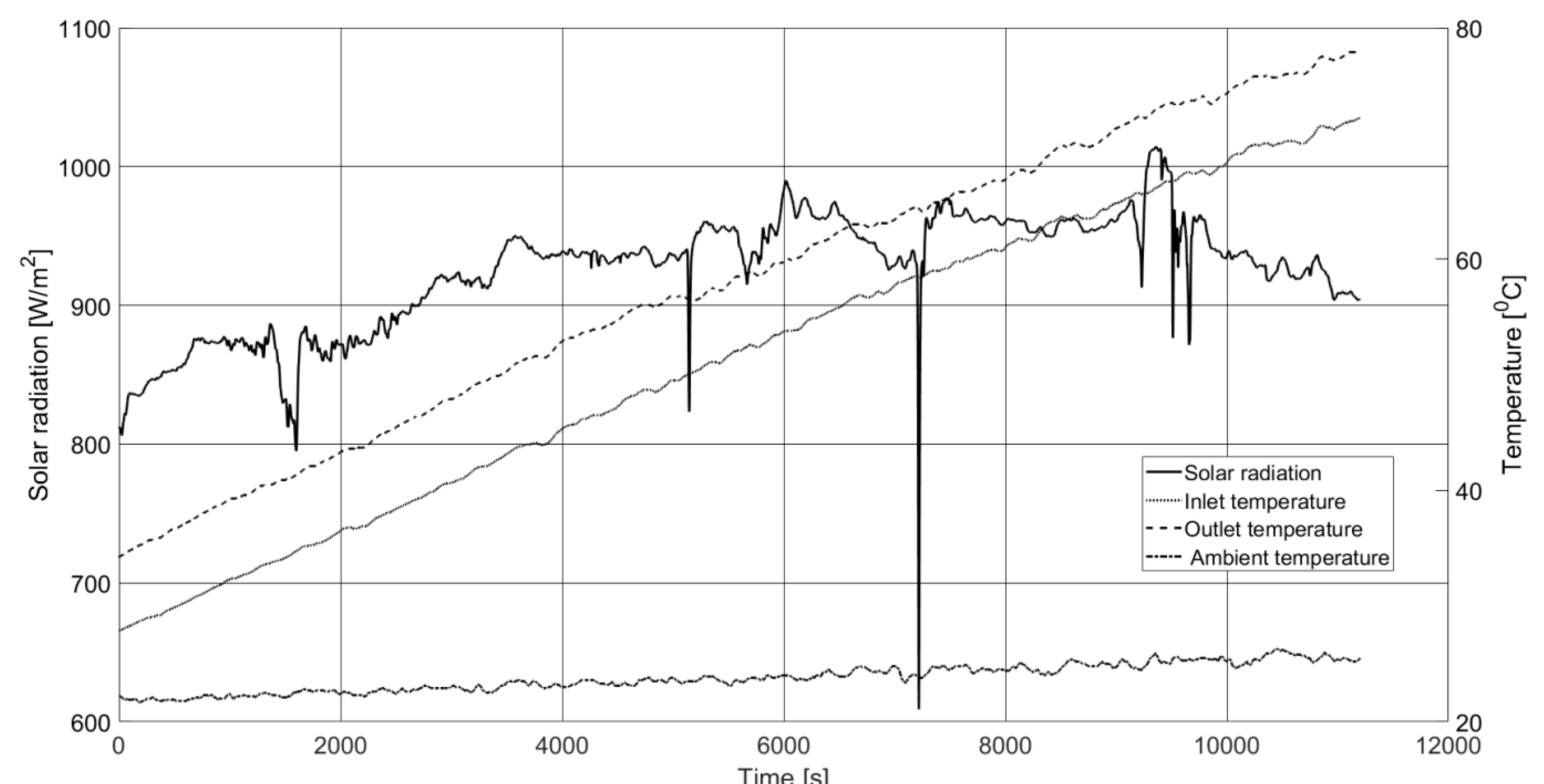
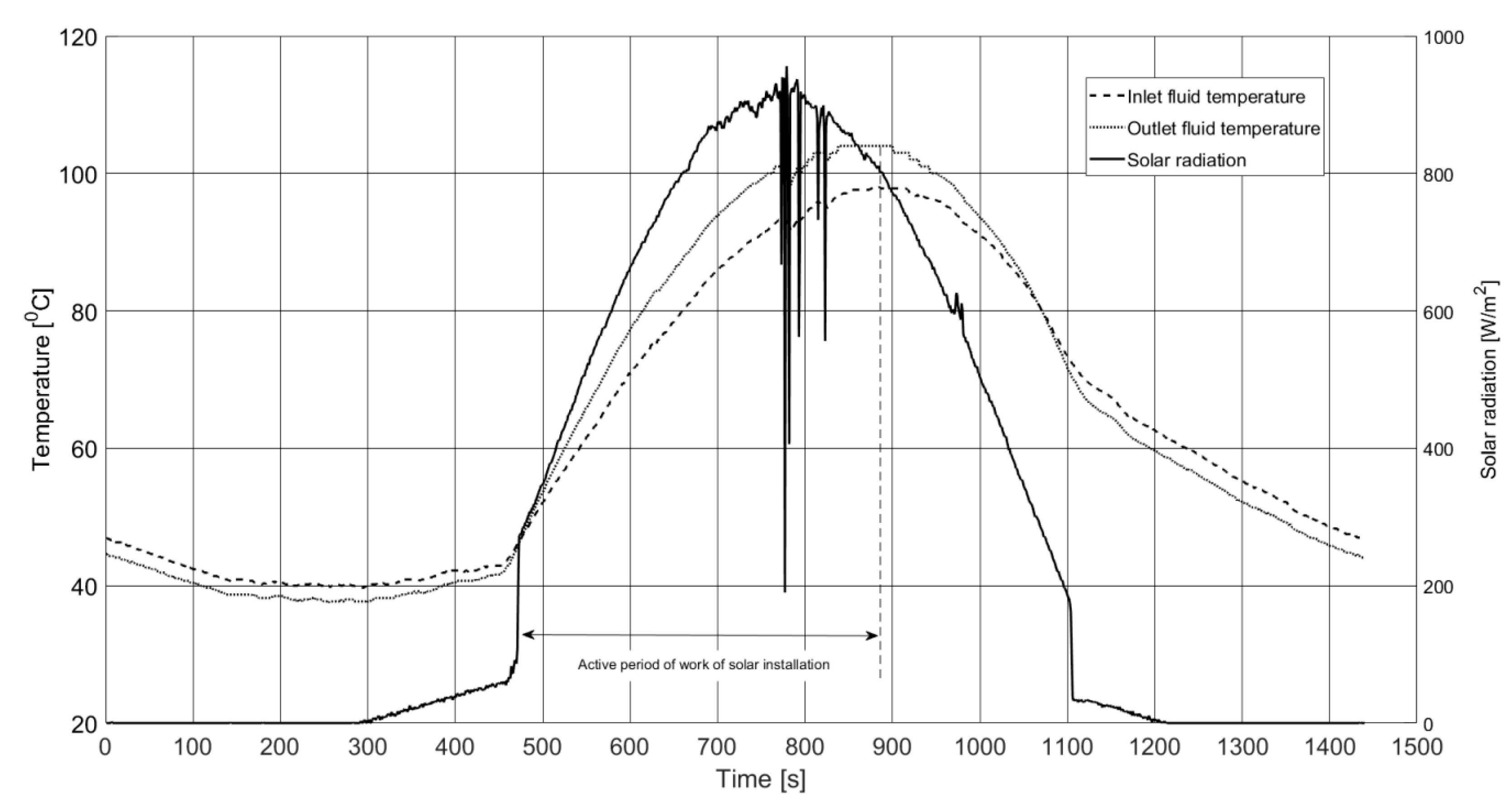
The method developed by Obstawski enables diagnostics of solar collectors working in large installations, such as the one presented in Figure 5. In practice, for such heating systems, the volume flow through the collector results from numerous factors, e.g., from the method of collector interconnections, and it is usually different from the standard flow rate. This method enables the values of characteristic parameters that were calculated for flow rate under operating conditions to be recalculated using the flow rate value according to the ISO 9806:2017 standard [6]. The experiment was performed for a constant volume flow rate in the system which equaled 0.41 dm³/s. When assuming a uniform flow of medium through specific sections, it may be estimated that the flow of medium through one collector amounted to 0.0208 dm³/s, thus being nearly 50% lower than during standard tests. Figure 15 shows the values of solar irradiance and the temperature of medium during the experiment. Due to the fact that the solar heating system is a segment of a hybrid power supply system based on a compressor heat pump, the automatic control system allows effective operation of the system once a temperature of 40 °C is exceeded in the hot water storage tank, which is the initial temperature of the working medium.

Based on the recorded measurement data using the parametric identification method, a model was created in the form of differential Equation (27), which was verified and then transformed, using Tustin’s method, into a continuous one, and it was approximated to an operator transform form described by Equation (28).

A(z) = 1 − 0.772 z⁻¹ − 0.2132 z⁻² + 0.07099 z⁻³
B1(z) = 0.00264 z⁻¹ − 0.0006327 z⁻²
B2(z) = 0.1621 z⁻¹ − 0.09136 z⁻²

(27)

$${\mathrm{T}}_{\mathrm{fo}}\left(\mathrm{s}\right)=\frac{0.0154}{298.35\mathrm{s}+1}\times {\mathrm{I}}_{\mathrm{T}}\left(\mathrm{s}\right)+\frac{0.947}{298.35\mathrm{s}+1}\times {\mathrm{T}}_{\mathrm{fi}}\left(\mathrm{s}\right)$$

(28)

Having the values of the gain coefficient and the time constant substitute, the characteristic parameters of the collector, collector efficiency characteristics Equation (29) and the time constant were determined (Table 2).

η = 0.417 − 1.533 T_m − 4.36 T_m²

(29)

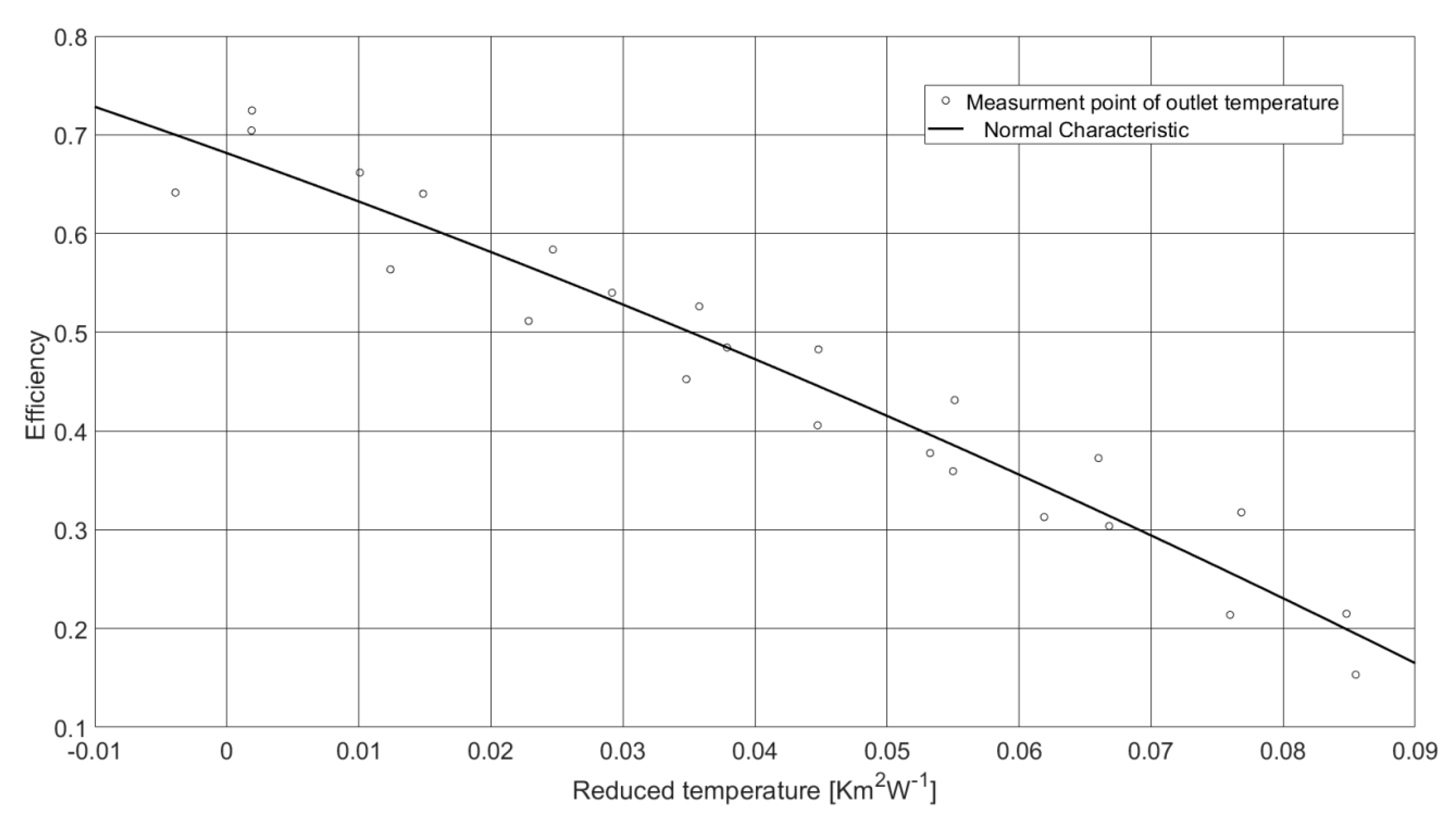
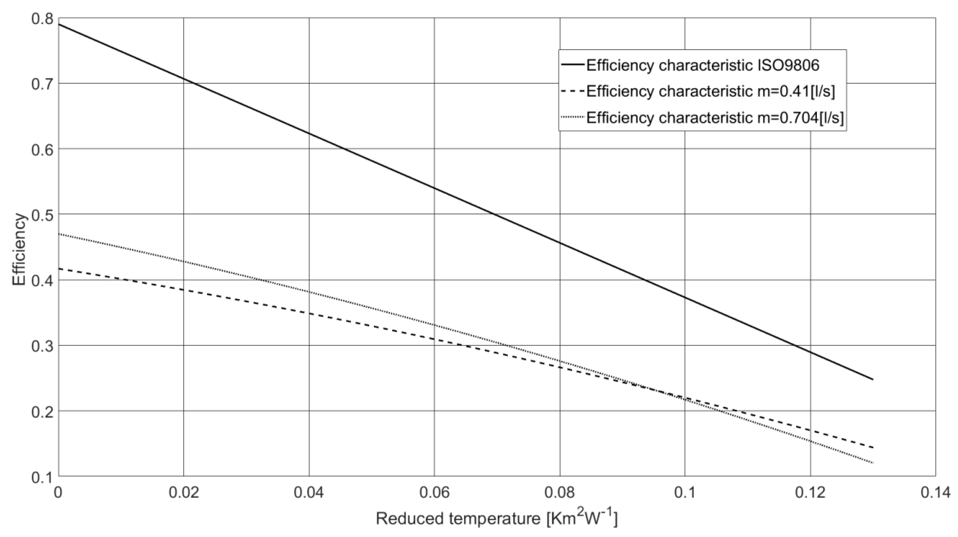
However, it should be noticed that the flow of medium through the collector in the modeled battery was two times lower than during standard tests. Knowing the value of the heat removal coefficient F_R, the coefficient of heat losses U_L, the battery aperture area A_C and the specific heat of the medium, by means of the equations (Table 1, item 30), it is possible to determine the efficiency characteristics of the collector batteries for the standard flow rate, which, for the analyzed collector battery, is 0.704 dm³/s (Figure 16). By increasing the flow rate up to the value from the ISO 9806:2017 [6] test standard, the modeled collector can be described using the transfer function Equation (30).

$${\mathrm{T}}_{\mathrm{fo}}\left(\mathrm{s}\right)=\frac{0.0077}{149.16\mathrm{s}+1}\times {\mathrm{I}}_{\mathrm{T}}\left(\mathrm{s}\right)+\frac{0.97}{149.16\mathrm{s}+1}\times {\mathrm{T}}_{\mathrm{fi}}\left(\mathrm{s}\right)$$

(30)

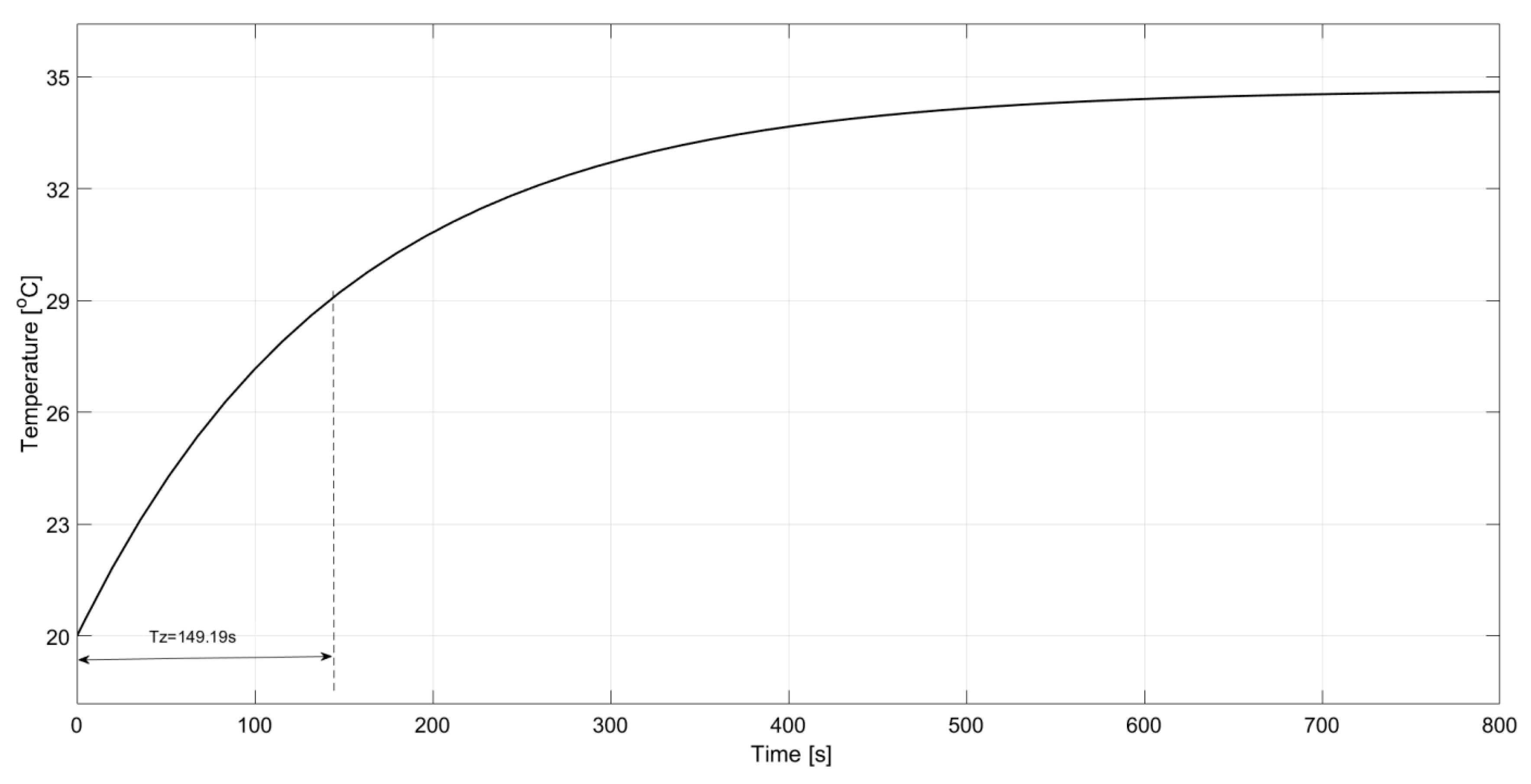
Figure 17 shows step characteristics of the modeled solar collector. The flow rate of fluid impacts the value of the time constant. An increase in the flow rate of fluid decreases the value of the time constant and increases the value of solar collector gain, which can be observed when analyzing collector model parameters after calibration (an increase in the flow rate of fluid) (Figure 16) (Table 2).

η = 0.47 − 2.001 T_m − 5.289 T_m²

(31)

5. Analysis of the Results and Discussion

When analyzing the parameters of a flat solar collector that has been tested using different methods, it should be noticed that the values of specific parameters are different. The biggest differences in the values of solar collector efficiency occur when the collector is thermally loaded with a large buffer tank (test stand II). A difference in the value of collector efficiency between an indoor test performed in accordance with the ISO 9806 standard and the parametric identification method developed by Obstawski for the operating conditions reaches up to 40%. A difference in the value of collector efficiency between the indoor test of the ISO 9806 standard and other methods is smaller and reaches 4%. An almost identical situation occurs in the case of values of the F_R, F’ and U_L coefficients. The smallest difference in the value of the F_R, F’ and U_L coefficients is observed between the normative methods (the ISO 9806 standard) and the ETN method (developed by Chochowski). The difference ranges between 2% and 20%. When comparing values of the F_R, F’ and U_L coefficients to their values calculated under operating conditions, the difference is higher, nearly 50%, e.g., for the value of the U_L coefficient. When analyzing the value of the time constant calculated using various methods, significant similarities can be observed only for the ISO 9806 standard and the ETN method. In other methods, the difference in the value of the time constant reaches up to 270% (the ISO 9806 standard and test stand I) (

Table 3. Comparison of the characteristic parameters of collectors based on different methods.

Method	Normal Characteristics	Effective Heat Capacity [kJ/m2K]	FR [-]	F’ [-]	UL [W/m2K]	Time Constant Tz (s)	Flow through the Collector dm3/min	Working Medium	Solar Irradiance W/m2
ISO 9806 indoor	η = 0.79 − 4.17Tm− 0.01Tm2	6.73	0.94	0.95	4.17	80	2.07	water	1000
ISO 9806 outdoor	η = 0.77 − 4.92Tm − 54.8Tm2	14.3	0.8	0.81	4.92	171	2.16	water	806 ± 5W
ETN Chochowski	η = 0.71 − 4.07Tm − 0.0001Tm2	6.71	0.75	0.76	4.07	77	2.16	water	1000
PI Obstawski installation I	η = 0.68 − 4.8Tm − 10.0Tm2	14.6	0.66	0.67	3.59	207.9	2,07	glycol	1000
PI Obstawski installation II	η = 0.417 − 1.533Tm − 4.36 Tm2	10.47	0.54	0.55	2.07	298.35	1.24	glycol	1000
PI Obstawski installation II (after calibration)	η = 0.47 − 2.001 Tm − 5.289 Tm2	10.47	0.54	0.55	2.07	149.19	2.07	glycol	1000

).

The time constant value is a very important parameter when designing the control system of a solar installation. An error in the calculation of the time constant can cause a decrease in the efficiency of a solar installation, and in the case of hybrid energy systems it can increase the consumption of a conventional energy carrier. This error can also cause unstable operation of the solar installation. Differences in the values of particular coefficients calculated using different methods are probably the results of nonlinear static characteristics of solar heating installations. Each method is based on linear models in the form of differential equations. Each operating point change in a solar installation described by the parameters of work—e.g., the inlet and outlet fluid temperature, the value of solar irradiance, the ambient temperature—has influence on the value of the coefficients of a solar collector model. This can be observed when analyzing the results provided by the ISO 9806 standard, both indoor and obtained in the ETN methods.

Calculations of the characteristic coefficients of a solar collector in both methods, e.g., the time constant, the effective heat capacity and heat loss, are convergent. This is a result of very stable and steady conditions during the experiments. In the case of the ISO 9806 standard indoor, experiments are performed under indoor conditions using a simulator of solar irradiance. In the case of ETN, the parameters of ETN are calculated based on the values of the coefficients of each solar collector component material, and the values of characteristic parameters of the collector are the result of computer simulations. In the case of other methods, the parameters vary. Even in the case of the outdoor method according to the ISO 9806 standard, the parameters change insignificantly (they are quasi-stabile) during experiments. As a result, designing the control systems of solar installations requires an adaptive control algorithm enabling calculation of the values of operating parameters in a solar heating system in real time. The biggest limitation of the presented and tested methods except the ISO 9806:2017 standard involves the fact of omitting the delay time, which is very important when designing a control system, because the response of a controlled object, such as a solar collector, can be in the same time as the command.

6. Conclusions

Based on the performed analyses, it shall be concluded that the static and dynamic properties of a flat-plate solar collector are variable and depend on prevailing operating conditions. When considering the parameters of a collector determined during standard tests (ISO 9806 indoor) as reference values, it shall be noticed that the most similar results concerning efficiency were produced using the ISO 9806 outdoor and the ETN methods. In the case of a collector heat loaded with a hot water storage tank, the efficiency of the collector is lower than the reference value. Similar conclusions may be formulated when analyzing the values of other parameters characterizing the steady state of the collector–F’, F_R and U_L. The heat capacity value of the collector and the resulting time constant substitute depend not only on structural parameters (similar results of the ISO 9806 standard indoor and the ETN method), but also on other factors, for instance related to the system structure and the collector heat load, the temperature of fluid, i.e., parameters defining the operating point of a solar heating installation that vary under operating conditions. Optimizing the operation of a solar heating installation requires developing an adaptive control algorithm enabling real-time calculations of characteristic parameters of the solar installation, e.g., the time constant, the delay time under operating conditions.

References

- Diez, F.J.; Navas-Gracia, L.M.; Martinez-Rodriguez, A.; Correa-Guimaraes, A.; Chico-Santamarta, L. Moddeling of flat-plate solar collector using artificial neural network for different working fluid (water) flow rates. Sol. Energy 2019, 188, 1320–1331. [Google Scholar] [CrossRef]
- Banos, R.; Manzano-Agugliaro, F.; Montoyab, F.G.; Gil, C.; Alcayde, A.; Gómez, J. Optimization methods applied to renewable and sustainable energy: A review. Renew. Sustain. Energy Rev. 2011, 15, 1753–1766. [Google Scholar] [CrossRef]
- Sharma, N.; Varun, S. Stochastic techniques used for optimization in solar systems: A review. Renew. Sustain. Energy Rev. 2012, 16, 1399–1411. [Google Scholar] [CrossRef]
- Fan, M.; Zheng, W.; You, S.; Zhang, H.; Jiang, Y.; Wu, Z. Comparision of different dynamic thermal performance prediction models for the flat-plate solar collector with a new V-corrugated absorber. Sol. Energy 2020, 204, 406–418. [Google Scholar] [CrossRef]
- Carmona, M.; Palacio, M. Thermal modeling of a flat plate solar collector with laten heat storage validate with experimental data in outdoor conditions. Sol. Energy 2019, 177, 620–633. [Google Scholar] [CrossRef]
- Marrasso, E.; Roselli, C.; Sasso, M.; Tarioello, F. Analysis of a hybrid solar-assisted trigeneration system. Energies 2016, 9, 705. [Google Scholar] [CrossRef] [Green Version]
- Chochowski, A.; Czekalski, D.; Obstawski, P. Monitoring of renewable energy sources hybrid system operation. Electr. Rev. 2009, 8, 92–95. (In Polish) [Google Scholar]
- Hou, H.J.; Wang, Z.F.; Wang, R.Z.; Wang, P.M. A new method for the measurement of solar collector time constant. Renew. Energy 2005, 30, 855–865. [Google Scholar] [CrossRef]
- Saltiel, C.; Sokolov, M. Optimal control of a multicomponent solar collector system. Sol. Energy 1985, 34, 463–473. [Google Scholar] [CrossRef]
- Araújo, A.; Silva, R.; Pereira, V. Solar thermal modeling for rapid estimation of auxiliary energy requirements in domestic hot water production: On-off versus proportional flow rate control. Sol. Energy 2019, 177, 68–79. [Google Scholar] [CrossRef]
- Morteza, A.; Ardehali, M.; Yae, K.H.; Smith, T.F. Development of proportional-sum-derivative control methodology. Sol. Energy 1996, 57, 251–260. [Google Scholar]
- Winn, C.B. Controls in Solar Energy Systems, an Annual Review of Research and Development; Springer: London, UK, 1982; Volume 1, pp. 209–240. [Google Scholar]
- Löf, G. Active Solar Systems; MIT Press: Cambridge, MA, USA, 1993. [Google Scholar]
- Badescu, V. Optimal control of flow in solar collector systems with fully mixed water storage tanks. Energy Convers. Manag. 2008, 49, 169–184. [Google Scholar] [CrossRef]
- Budea, S.; Bădescu, V. Improving the Performance of Systems with Solar Water Collectors used in Domestic Hot Water Production. Energy Procedia 2017, 112, 398–403. [Google Scholar] [CrossRef]
- Bettoni, D.; Soppelsa, A.; Fedrizzi, R.; Del Toro Matamoros, R.M. Analysis and Adaptation of Q-Learning Algorithm to Expert Controls of a Solar Domestic Hot Water System. Appl. Syst. Innov. 2019, 2, 15. [Google Scholar] [CrossRef] [Green Version]
- ISO 9459-4:2013—Solar Heating—Domestic Water Heating Systems—Part 4: System Performance Characterization by Means of Component Tests and Computer Simulation; European Committee for Standardization: Brussels, Belgium, 2013.
- ASHRE Standard 93-77: Methods of Testing to Determine the Thermal Performances of Solar Collectors; American Society of Heating, Refrigerating and Air-Conditioning Engineers: Washington, DC, USA, 1997.
- EN 12975-1+A1:2010—Thermal Solar Systems and Components—Solar Collectors—Part 1: General Requirements; European Committee for Standardization: Brussels, Belgium, 2010.
- EN ISO 9806:2017—Solar Energy—Solar Thermal Collectors—Test Methods; European Committee for Standardization: Brussels, Belgium, 2017.
- Duffie, J.A.; Beckman, W.A. Solar Engineering of Thermal Processes; John Wiley & Sons: Hoboken, NJ, USA, 1991. [Google Scholar]
- Emery, M.; Rogers, B.A. On a solar collector thermal performance test method for use in variable conditions. Sol. Energy 1984, 33, 117–123. [Google Scholar] [CrossRef]
- Saunier, G.Y.; Chungpaibulpatana, S. A New inexpensive dynamic method of testing to determine solar thermal performance. In Proceedings ISES Solar World Congress, Australia; Szokolay, S.V., Ed.; Pergamon Press: New York, NY, USA, 1983; Volume 2, pp. 910–916. [Google Scholar]
- Wang, X.A.; Xu, Y.F.; Meng, X.Y. A filter method for transient testing of collector performance. Sol. Energy 1987, 38, 125–134. [Google Scholar] [CrossRef]
- Muschaweck, J.; Spirkl, W. Dynamic solar collector performance testing. Sol. Energy Mater. Sol. Cells 1993, 30, 95–105. [Google Scholar] [CrossRef]
- Chungpaibulpatana, S.; Exell, R.H.B. The effects of using a one-node heat capacitance model for determining solar collector performance parameters by transient test methods. Sol. Wind Technol. 1988, 5, 411–421. [Google Scholar] [CrossRef]
- Perers, B. Dynamic method for solar collector array testing and evaluation with standard database and simulation programs. Sol. Energy 1993, 50, 517–526. [Google Scholar] [CrossRef]
- Wijeysundera, N.E.; Hawlade, M.N.A.; Foong, K.Y. Estimation of collector performance parameters from daily system test. Sol. Energy 1996, 118, 30–36. [Google Scholar] [CrossRef]
- Amer, E.H.; Nayak, J.K.; Sharma, G.K. A transient test methods for flat-plate collectors. Energy Convers. Manag. 1998, 39, 549–558. [Google Scholar] [CrossRef]
- Amer, E.H.; Nayak, J.K.; Sharma, G.K. A new dynamic method for testing of flat-plate solar collectors. Energy Convers. Manag. 1999, 40, 803–823. [Google Scholar] [CrossRef]
- Kong, W.; Wang, Z.; Li, X.; Li, X.; Xiao, N. Theoretical analysis and experimental verification of a new dynamic test method for solar collectors. Sol. Energy 2012, 86, 398–406. [Google Scholar] [CrossRef]
- Buzás, J.; Kicsiny, R. Transfer functions of solar collectors for dynamical analysis and control design. Renew. Energy 2014, 68, 146–155. [Google Scholar] [CrossRef]
- Deng, J.; Yang, X.; Wang, P. Study on the second-order transfer function models for dynamic tests of flat-plate solar collectors Part I: A proposed new model and a fitting methodology. Sol. Energy 2015, 114, 418–426. [Google Scholar] [CrossRef]
- Deng, J.; Yang, X.; Wang, P. Study on the second-order transfer function models for dynamic tests of flat-plate solar collectors Part II: Experimental validation. Sol. Energy 2017, 141, 334–346. [Google Scholar] [CrossRef]
- Deng, J.; Xu, Y.; Yang, X. A dynamic thermal performance model for flat-plate solar collectors based on the thermal inertia correction of the steady-state test method. Renew. Energy 2015, 76, 679–686. [Google Scholar] [CrossRef]
- Deng, J.; Ma, R.; Yuan, G.; Chang, C.; Yang, X. Dynamic thermal performance prediction model for the flat-plate solar collectors based on the two-node lumped heat capacitance method. Sol. Energy 2016, 135, 769–779. [Google Scholar] [CrossRef]
- Amrizal, N.; Chemisana, D.; Rosell, J.I.; Barrau, J. A dynamic model based on the piston flow concept for the thermal characterization of solar collectors. Appl. Energy 2012, 94, 244–250. [Google Scholar] [CrossRef]
- Deng, J.; Yang, M.; Ma, R.; Zhu, X.; Fan, J.; Yuan, G.; Wang, Z. Validation of a simple dynamic thermal performance characterization model based on the piston flow concept for flat-plate solar collectors. Sol. Energy 2016, 139, 171–178. [Google Scholar] [CrossRef] [Green Version]
- Kamminga, W. Experiences of a solar collector test method using Fourier transfer functions. Heat Mass Transf. 1985, 28, 1393–1404. [Google Scholar] [CrossRef]
- Mintsa Do Ango, A.C.; Medale, M.; Abid, C. Optimization of the design of a polymer flat plate solar collector. Sol. Energy 2013, 87, 64–75. [Google Scholar] [CrossRef] [Green Version]
- Henning, H.M.; Sasse, M. A collector hardware simulator: Theoretical analysis and experimental result. Sol. Energy 1995, 55, 39–48. [Google Scholar] [CrossRef]
- Tsilingiris, P.T. Heat transfer analysis of low thermal conductivity solar energy absorbers. Appl. Therm. Eng. 2000, 20, 1297–1314. [Google Scholar] [CrossRef]
- Eisenmann, W.; Vajen, K.; Ackermann, H. On the correlations between collector efficiency factor and material content of parallel flow flat-plate solar collectors. Sol. Energy 2004, 76, 381–387. [Google Scholar] [CrossRef]
- Chochowski, A. Thermal States Analysis of a Flat-plate Solar Collector; SGGW Publishers: Warsaw, Poland, 1991. (In Polish) [Google Scholar]
- Farkas, I. Identification of flat plate solar collectors used in agriculture. In Proceedings of the 9th IFAC-IFORS Symposium; Bányász, C.S., Keviczky, L., Eds.; Elsevier: Budapest, Hungary, 1991; Volume 1, pp. 475–479. [Google Scholar]
- Cristofari, C.; Notton, P.; Louche, A. Modelling and performance of a copolymer solar water heating collector. Sol. Energy 2002, 72, 99–112. [Google Scholar] [CrossRef]
- Rodriguez-Hidalgo, M.C.; Rodriguez-Aaumente, P.A.; Lecuona, A.; Gutierrez-Ureta, G.L.; Ventas, R. Flat plate thermal solar collector efficiency: Transient behavior under working conditions. Part I: Model description and experimental validation. Appl. Therm. Eng. 2011, 31, 2394–2404. [Google Scholar] [CrossRef] [Green Version]
- Kalogirou, S.; Panteliou, S.; Dentsoras, A. Modelling of solar domestic water heating systems using artificial neural networks. Sol. Energy 1999, 65, 335–342. [Google Scholar] [CrossRef]
- Kalogirou, S.; Panteliou, S.; Dentsoras, A. Artificial neural networks used for the performance prediction of a thermosyphon solar water heater. Renew. Energy 1999, 18, 87–99. [Google Scholar] [CrossRef]
- Kalogirou, S.; Panteliou, S. Thermosyphon solar domestic water heating systems long-term performance prediction using artificial neural networks. Sol. Energy 2000, 69, 163–174. [Google Scholar] [CrossRef]
- Kalogirou, S. Long-term performance prediction of forced circulation solar domestic water heating systems using artificial neural networks. Appl. Energy 2000, 66, 63–74. [Google Scholar] [CrossRef]
- Li, H.; Liu, Z.; Liu, K.; Zhang, Z. Predictive power of machine learning for optimizing solar water heater performance: The potential application of high-throughput screening. Int. J. Photoenergy 2017. [CrossRef] [Green Version]
- Li, H.; Liu, Z. Performance prediction and optimization of solar water heater via a knowledge-based machine learning method. In Handbook of Research on Power and Energy System Optimization; IGI Global: Hershey, PA, USA, 2018. [Google Scholar]
- Ghritlahre, H.K.; Prasad, R.K. Application of ANN technique to predict the performance of solar collector systems—A review. Renew. Sustain. Energy Rev. 2018, 84, 75–88. [Google Scholar] [CrossRef]
- Farkas, I.; Geczy-Vig, P. Neural network modeling of flat-plate solar collectors. Comput. Electron. Agric. 2003, 40, 87–102. [Google Scholar] [CrossRef]
- Kalogirou, S.A. Prediction of flat-plate collector performance parameters using artificial neural networks. Sol. Energy 2006, 80, 248–259. [Google Scholar] [CrossRef]
- Sözen, A.; Melnik, T.; Unvar, S. Determination of efficiency of flat-plate solar collectors using neural network approach. Expert Syst. Appl. 2008, 35, 1533–1539. [Google Scholar] [CrossRef]
- Baccoli, R.; Carlini, U.; Mariotti, S.; Innamorati, R.; Solinas, E.; Mura, P. Graybox and adaptive dynamic neural network identification models to inter the steady state efficiency of solar thermal collectors starting from the transient condition. Sol. Energy 2010, 84, 1027–1046. [Google Scholar]
- Obstawski, P. Modeling the Dynamics of Work of a Flat-Plate Solar Collector. Ph.D. Thesis, Warsaw University of Life Sciences, Warsaw, Poland, 2007. (In Polish). [Google Scholar]
- Aleksiejuk, J.; Chochowski, A.; Reshetiuk, V. Analog model of dynamics of a flat-plate solar collector. Sol. Energy 2018, 160, 103–116. [Google Scholar] [CrossRef]
- Obstawski, P.; Bakoń, T.; Czekalski, D. Diagnostic method of solar thermal system based on the short time on-line measurements. Appl. Therm. Eng. 2019, 148, 420–429. [Google Scholar] [CrossRef]
Figure 1.
Thermal schema of the collector for a transient state.
Figure 2.
Block diagram of the solar segment model developed based on energy balance for a transient state.
Figure 3.
Test stand (system I).
Figure 4.
Visualization of work of test stand I in the Supervisory Control and Data Acquisition (SCADA) system.
Figure 5.
Test stand (system II).
Figure 6.
Visualization of work of test stand II in the SCADA system.
Figure 7.
The step response of the collector determined according to the ISO 9806:17 standard under outdoor conditions.
Figure 8.
Collector efficiency characteristics determined according to the ISO 9806 standard under outdoor conditions.
Figure 9.
The equivalent thermal network implemented in Simulink.
Figure 10.
The step response of the collector determined using the ETN method according to Chochowski.
Figure 11.
Efficiency characteristics of the collector determined using the ETN method.
Figure 12.
Solar irradiance and working medium temperature values in the system during the experiment.
Figure 13.
Efficiency characteristics of the collector heat loaded with a 100 dm3 storage tank.
Figure 14.
Step response of the collector heat loaded with a 100 dm3 storage tank.
Figure 15.
Solar irradiance and working medium temperature values in the system during the experiment (test stand II).
Figure 16.
Efficiency characteristics of a battery of 20 collectors heat loaded with a 1000 dm3 storage tank.
Figure 17.
Step response of a battery of 20 collectors heat loaded with a 1000 dm3 storage tank.