Computer-Aided Nonlinear Frequency Response Method for Investigating the Dynamics of Chemical Engineering Systems

Abstract

The Nonlinear Frequency Response (NFR) method is a useful Process Systems Engineering tool for developing experimental techniques and periodic processes that exploit the system nonlinearity. The basic and most time-consuming step of the NFR method is the derivation of frequency response functions (FRFs). The computer-aided Nonlinear Frequency Response (cNFR) method, presented in this work, uses a software application for automatic derivation of the FRFs, thus making the NFR analysis much simpler, even for systems with complex dynamics. The cNFR application uses an Excel user-friendly interface for defining the model equations and variables, and MATLAB code which performs analytical derivations. As a result, the cNFR application generates MATLAB files containing the derived FRFs in a symbolic and algebraic vector form. In this paper, the software is explained in detail and illustrated through: (1) analysis of periodic operation of an isothermal continuous stirred-tank reactor with a simple reaction mechanism, and (2) experimental identification of electrochemical oxygen reduction reaction.

1. Introduction

Knowledge about process dynamics is crucial in chemical engineering, as well as in other engineering fields. One of the particularly useful tools for investigating process dynamics is frequency response (FR) [1,2,3,4,5,6,7]. FR is a response of the investigated system to sinusoidal input modulation and it enables defining a convenient model form in the frequency domain, usually called frequency transfer function or frequency response function [8]. As a rule, the frequency transfer function is a linear model and can be used only for linear systems. On the other hand, the great majority of real systems are nonlinear, so nonlinear tools are necessary for their analysis. One such tool is the nonlinear frequency response method, which is used in this paper.

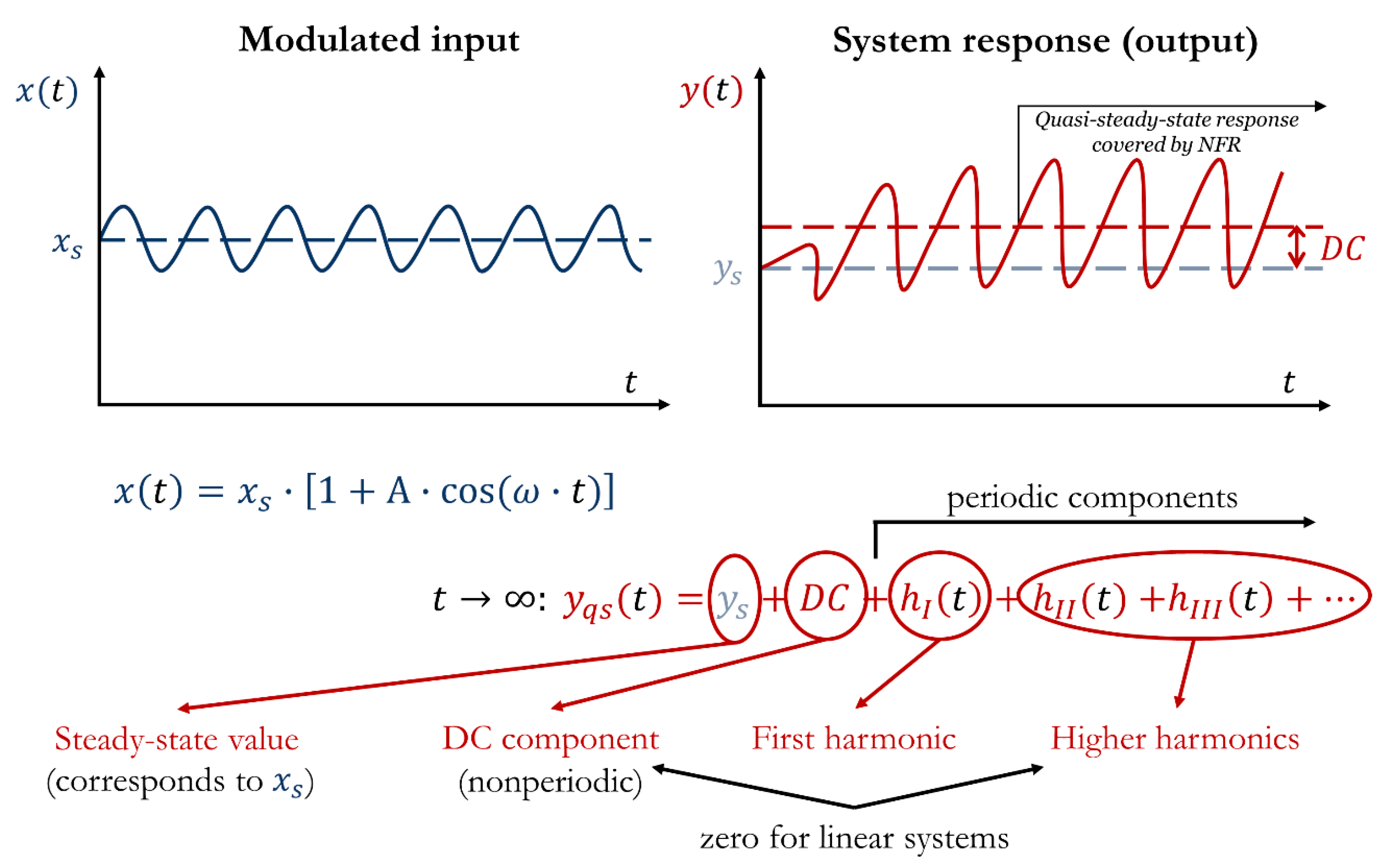
In our research, we use the term nonlinear frequency response (NFR) for a quasi-steady-state (often called periodic steady-state) response of a stable, weakly nonlinear system to a sinusoidal input change with a relatively high amplitude [9]. The quasi-steady-state response is obtained when the transient response of the system vanishes and it can be described as a sum of the first (basic) and, theoretically, an infinite number of higher harmonics, a nonperiodic (i.e., constant-in-time) term (DC component) and the steady-state operation value (Figure 1). For linear systems, or when the forcing amplitude is sufficiently small, both the DC component and all higher harmonics become zero.

In our investigations, we are using the NFR method based on the concept of higher-order frequency response functions (FRFs) [9]. This approach is mathematically based on the Volterra series [10] and multidimensional Fourier transform [11]. Thus, it can be applied only on systems that can be represented with convergent Volterra series [12]. Another limitation is that the analyzed systems must be stable with no multiple steady states [13], and weakly nonlinear [9], for which all nonlinear terms can be expressed as Taylor series expansions. In other words, all terms in the model equations must be continuous and differentiable functions [9].

The NFR method replaces the nonlinear dynamic model of a weakly nonlinear system with a set of FRFs of the first, second, and higher orders [9,14]. For an exact representation of the nonlinear model, an infinite sequence of FRFs would be needed, but approximations using only the first and second, or eventually third-order FRFs have shown very good results [15,16,17,18,19,20,21,22,23,24,25,26,27,28,29].

The NFR method has been proven to be an excellent analytical process systems engineering (PSE) tool for analyzing nonlinear dynamic systems in the field of chemical engineering. Our research using the NFR analysis was developed in three main directions:

1.

Developing experimental techniques for investigating process equilibrium and kinetics and estimating the related parameters.

The research was mainly focused on developing NFR methods for investigating adsorption [14,15,17,24,28,29,30,31,32,33,34,35,36,37,38] and electrochemical systems [21,22,23,39], although a similar approach could be used for other applications. These methods can be considered as extensions of the corresponding linear FR methods (classical FR technique for investigating adsorption kinetics, first introduced by Naphtali and Polinski [40], or the classical Electrochemical Impedance Spectroscopy (EIS), first introduced by Epelboin and Loric [41]). The main advantage of our NFR approach is that the second-order FRFs enable mechanism discrimination, based on distinctive shapes of the corresponding amplitude and phase characteristics corresponding to different mechanisms, even in cases when different mechanisms have essentially identical shapes of the first order FRFs [15,16,21,42]. The process mechanism is identified by comparing the FRFs estimated from experimental NFR measurements with the theoretical FRFs corresponding to different mechanisms in consideration. Besides that, the higher-order FRFs contain additional information that can be used for estimating the parameters of the identified process mechanism. Therefore, both the equilibrium and kinetic parameters can be estimated [43]. The NFR techniques for investigating adsorption and electrochemical systems were first developed theoretically [14,15,17,19,20,21,22,24,28,30,31,32,33,35,38] and then applied and verified experimentally [23,29,34,37,39].

2.

Developing a computational method for direct prediction of the periodic steady-state of cyclic processes.

This approach was used for predicting the complete temporal profiles of the process variables in the periodic steady-state, for inherent periodic processes which can be operated only in the periodic mode (usually called cyclic processes), such as adsorption cycles [18]. The process variables are computed using the previously derived theoretical FRFs and all computations are performed in the frequency domain, using only simple algebra. In this way, numerical solutions of the nonlinear model equations, which can be long and tedious, especially for slow systems with long transient times, are avoided. The method is analytical and essentially approximate, as only a finite number of FRFs of the analyzed system are used. Nevertheless, it was shown that even predictions based only on the first three FRFs showed reasonably good agreement with numerical simulations [18].

3.

Developing a method for fast and easy evaluation of possible enhancement of process performances through forced periodic modulations of the system inputs.

This method uses the NFR analysis for predicting the time-average values of the process outputs of interest in the periodic steady-state, which are directly related to the DC component shown in Figure 1. This method is also analytical and essentially approximate, but it was shown that very good predictions of the time-average behavior in the periodic steady-state can be obtained by using only the asymmetrical second-order FRFs [20,25,26,27,44,45,46,47,48,49,50,51]. Up to now, the applications were limited to the analysis of periodically operated chemical reactors. The method was successfully applied to isothermal [20,25,50] and nonisothermal [26,27,45,46,47,48] reactors, with one [20,26,27,50] or two [25,45,46,47,48] modulated inputs, for sinusoidal [20,25,26,45,46,48,50,51] or any other shapes [47,52] of the modulated inputs. In addition to the answer whether the periodic operation can be superior to the corresponding steady-state operation, the NFR analysis enables finding the best set of input forcing parameters (frequency, amplitudes, and phase difference in the case of two inputs) for the chosen performance criteria, e.g., conversion, yield, selectivity, etc. [44].

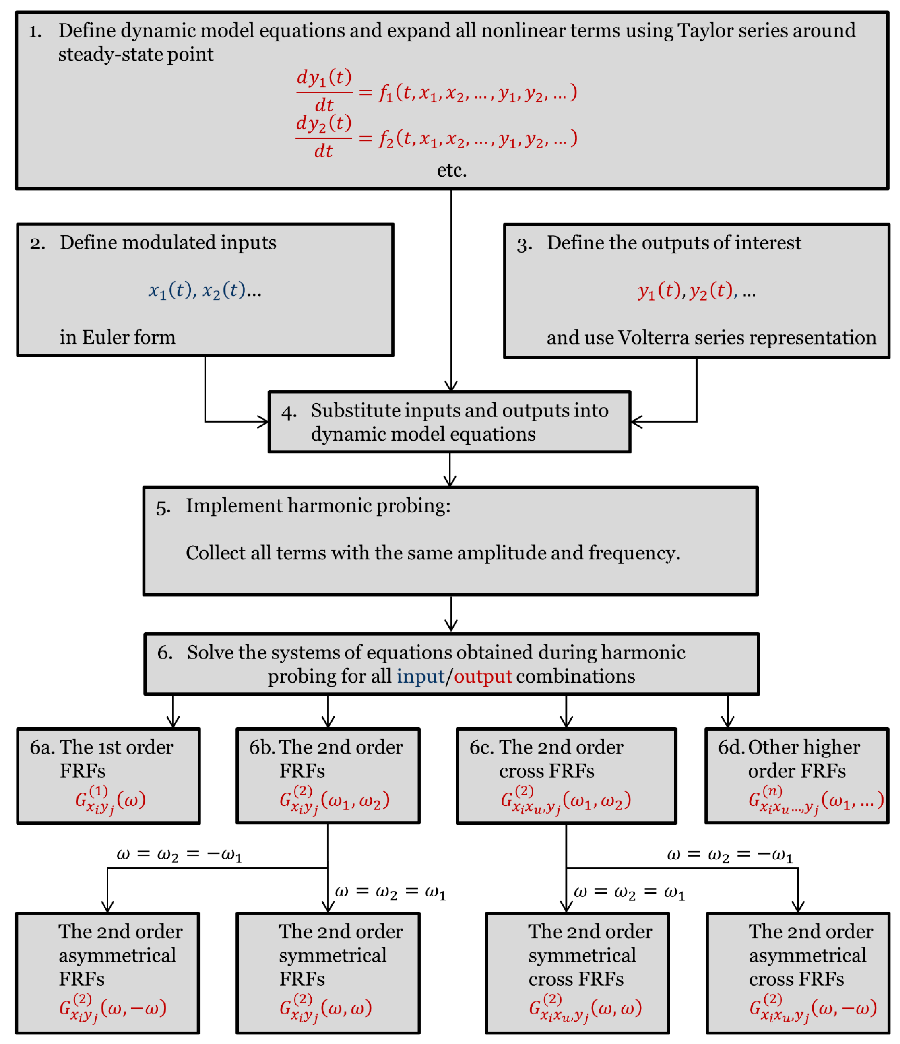
All these applications are based on theoretical FRFs which need to be derived from a relevant nonlinear dynamic model. The procedure for derivation of the theoretical FRFs is clear, well established, and documented in a number of our previous publications [18,20,21,22,53]. It is schematically shown in Figure 2.

Most of the steps shown in Figure 2 are self-explanatory. In Step 5, harmonic probing is performed by collecting all terms of the same frequency and power of the input amplitude and equating them to zero. This is a crucial step in which the analysis is transferred from time- to frequency domain and the set of nonlinear ODEs is replaced by a larger set of linear algebraic equations.

The following notation for the FRFs is used in Figure 2 and throughout this paper: $G_{x_i,y_j}^{\left(1\right)}\left(\omega \right)$ the first-order FRF relating output $y_j$ and input $x_i$,$G_{x_i,y_j}^{\left(2\right)}\left({\omega }_1,{\omega }_2\right)$ the second-order FRFs relating output $y_j$ and input $x_i$ and $G_{x_i{x}_u,y_j}^{\left(2\right)}\left({\omega }_1,{\omega }_2\right)$ the cross second-order FRF relating output $y_j$ to inputs $x_i$ and $x_u$.

In most cases, it is convenient to define the inputs and outputs in a dimensionless form, as relative deviations from their steady-state values:

$$X_i=\frac{x_i-x_{i,s}}{x_{i,s}}, Y_j=\frac{y_j-y_{j,s}}{y_{j,s}}$$

(1)

As a consequence, the derived FRFs are also dimensionless, as well as the input amplitudes which are always in the range between 0 and 1.

In Figure 2 the procedure is shown in detail for the derivation of the FRFs up to the second order. Nevertheless, it can easily be extended to the derivation of higher-order FRFs. The derivation procedure is recursive (the first-order FRFs are derived first, then the second-order FRFs, etc.) [14,20].

Although this procedure does not use any sophisticated mathematical tools, the derivation of the analytical expressions of the FRFs requires time, diligence, and specific mathematical skills from the user, especially for complex systems defined with large sets of differential equations and with several input/output combinations that need to be considered.

This work presents an advancement of the NFR method, the so-called computer-aided Nonlinear Frequency Response (cNFR), which uses a user-friendly software application for automatic derivation of the needed FRFs. The application will be explained in detail and its use illustrated in two examples.

2. Software Application for Computer-Aided Nonlinear Frequency Response Method

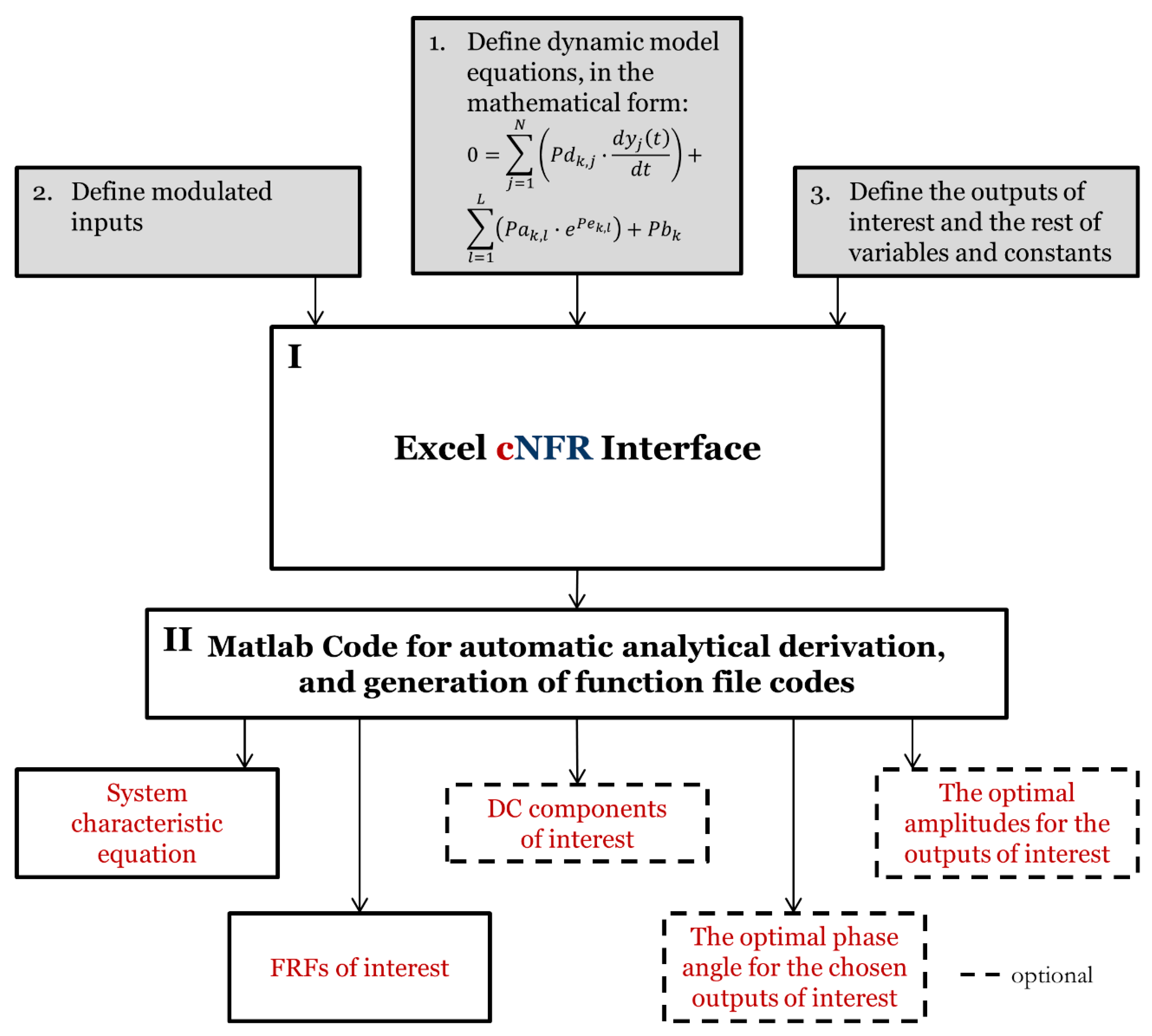
The structure of software application for the computer-aided Nonlinear Frequency Response (cNFR) method for automatic derivation of the needed FRFs, which upgraded our previously developed Nonlinear Frequency Response (NFR) method, is shown in Figure 3. The application consists of two linked segments: an Excel template which serves as a user interface and a MATLAB 2019b (MathWorks, Natick, MA, USA) program that performs the symbolic mathematical computations executing the derivation procedure shown in Figure 2 (Section 1).

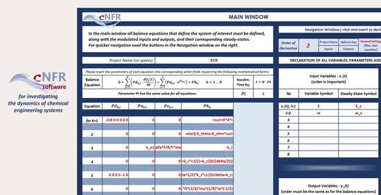
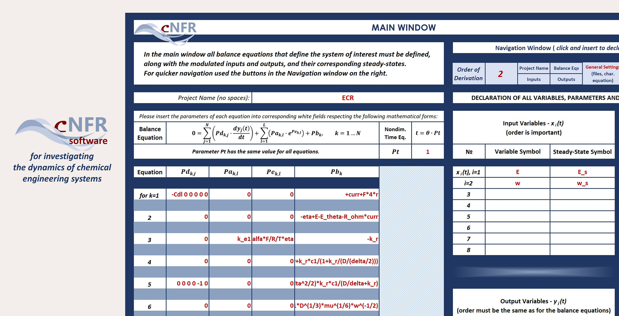
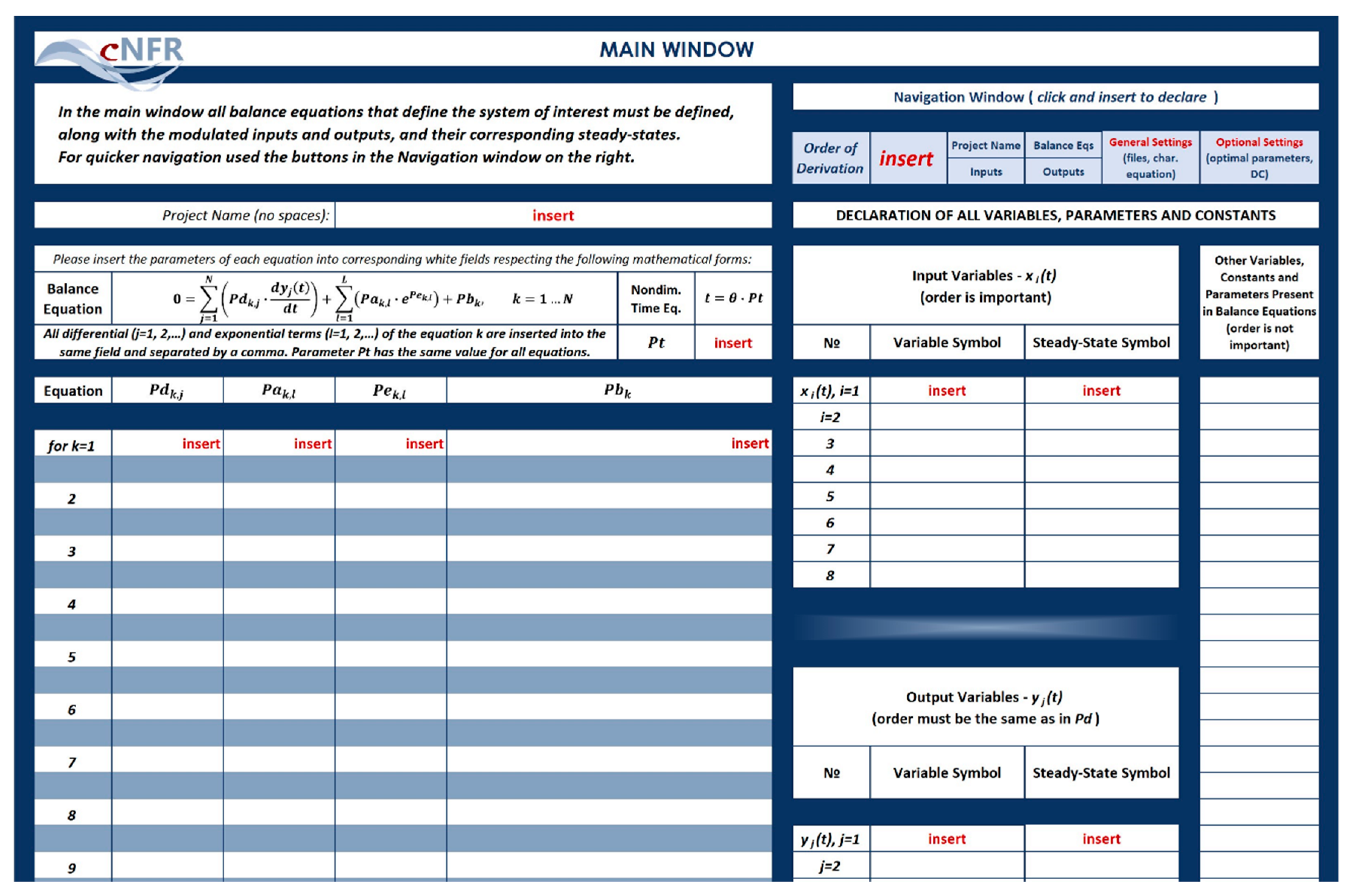
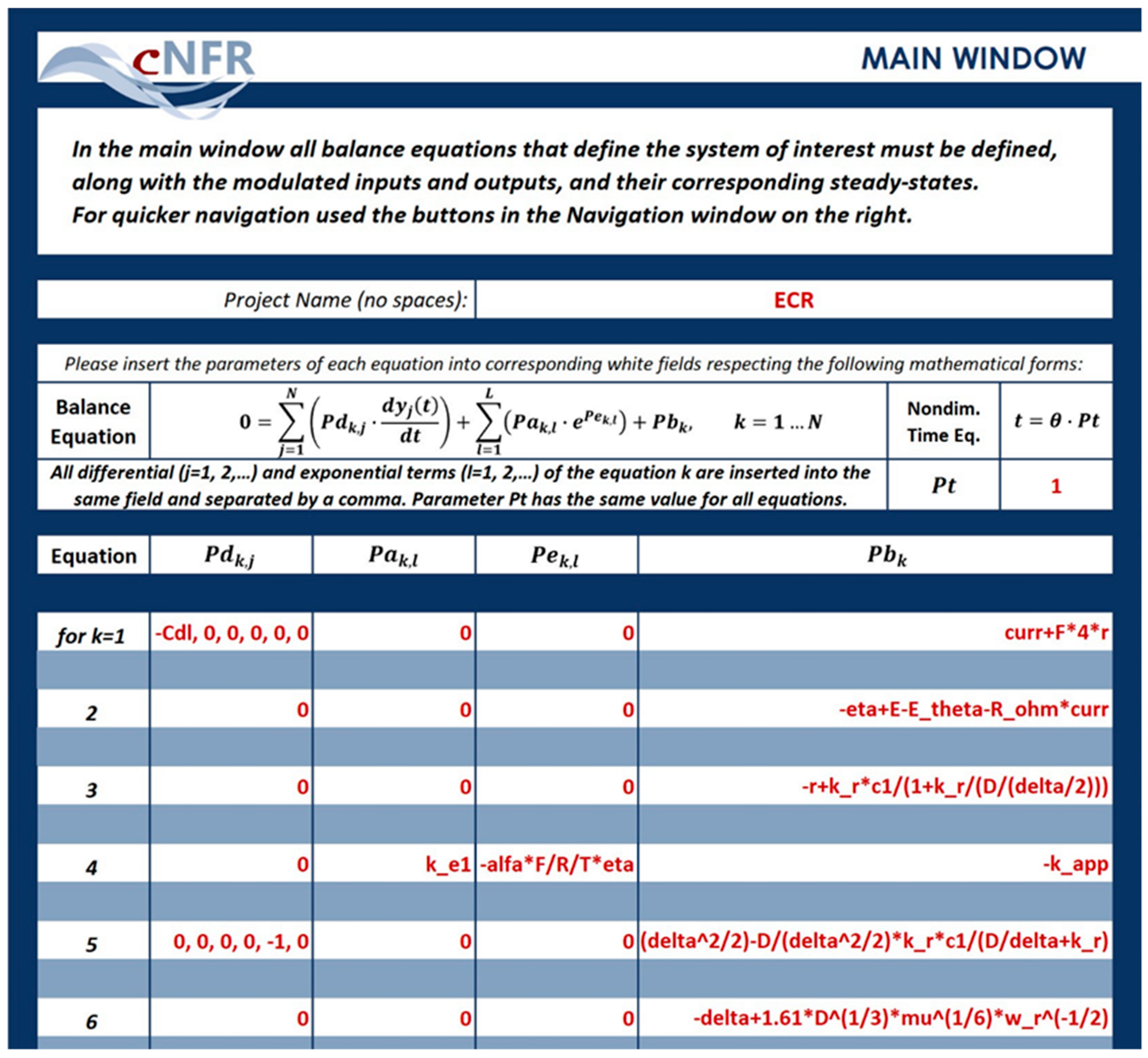
The cNFR Excel interface consists of two different windows. The cNFR Main Window (shown in Figure 4) is used for defining the model equations, the modulated inputs, the outputs of interest, as well as all system variables and model parameters. In the current version, the model equations need to be defined as a set of ODEs and algebraic equations. In the case of distributed parameter systems (described by sets of PDEs), the model PDEs need to be discretized before using the cNFR application.

The following general form of the model equations was chosen (Figure 4):

$$0={\displaystyle \sum }_{j=1}^N\left(P{d}_{k,j}·\frac{d{y}_j\left(t\right)}{dt}\right)+{\displaystyle \sum }_{l=1}^L\left(P{a}_{k,l}·e^{P{e}_{k,l}}\right)+P{b}_k, k=1\dots N$$

(2)

where $N$ is the total number of equations (same as the total number of all possible outputs $y_j$), $L$ is the maximal number of exponential terms, while $P{d}_{k,j}$, $P{a}_{k,l}$, $P{e}_{k,l}$ and $P{b}_k$ are, in principle, rational functions of time, input, and output variables, defined for each equation $k$. All this information is supplied by the user on the left-hand side of the cNFR interface Main Window, shown in Figure 4. The parameter $P{b}_k$ is inserted as one function-term, while parameters $P{d}_{k,j}$, $P{a}_{k,l}$, and $P{e}_{k,l}$ are inserted as vectors of function-terms. In a system with $N$ model equations, all differential terms of equation $k$ must be separated by commas or spaces and defined in each $P{d}_{k,j}$ field as a vector. If there are no differential terms in the balance equation, the user can just insert one zero. Analogously, if $L$ different exponential terms are present in the balance equation $k$, then all of these terms have to be defined in the same fashion as the differential terms, separated by commas or spaces, in the corresponding $P{a}_{k,l}$ and $P{e}_{k,l}$ vector fields. How the parameters $P{d}_{k,j}$, $P{a}_{k,l}$, and $P{e}_{k,l}$ are defined in practice will be demonstrated in two examples in Section 3.

Additionally, the user can choose to perform analysis with a dimensionless time, by setting a parameter $Pt$ which defines the relation between dimensional ($t$) and dimensionless time ($\theta$) as:

$$t=\theta ·Pt$$

(3)

If$Pt=1$, the dimensional time is assumed. It should be noted that the choice of the parameter $Pt$ reflects on the dimensions of the frequency which is the independent variable for the derived FRFs. For dimensional time ($Pt=1$), the corresponding frequency is dimensional, $\omega$ (e.g., rad/s or rad/min). On the other hand, if nondimensional time is used, the corresponding frequency will also be nondimensional, ${\omega }_{nd}$.

On the right-hand side of the cNFR Main Window (Figure 4), the user defines the input variables, $x_i\left(t\right)$, and the output variables, $y_j\left(t\right)$. The order ($j$) of defining output variables must match the order of elements in vector $P{d}_{k,j}$, and vice versa. The inputs and outputs are inserted in their original, dimensional form. The cNFR application automatically transforms them into dimensionless form (as relative deviations from their steady-state values, according to Equation (1)). It is not necessary to declare explicitly other variables, constants, and parameters in the Main Window, as the cNFR application will define all used symbols automatically in the complex domain. However, if the parameters are declared, they are treated as real values, which can be useful and potentially shorten the computing time for the automatic procedure of FRF derivation.

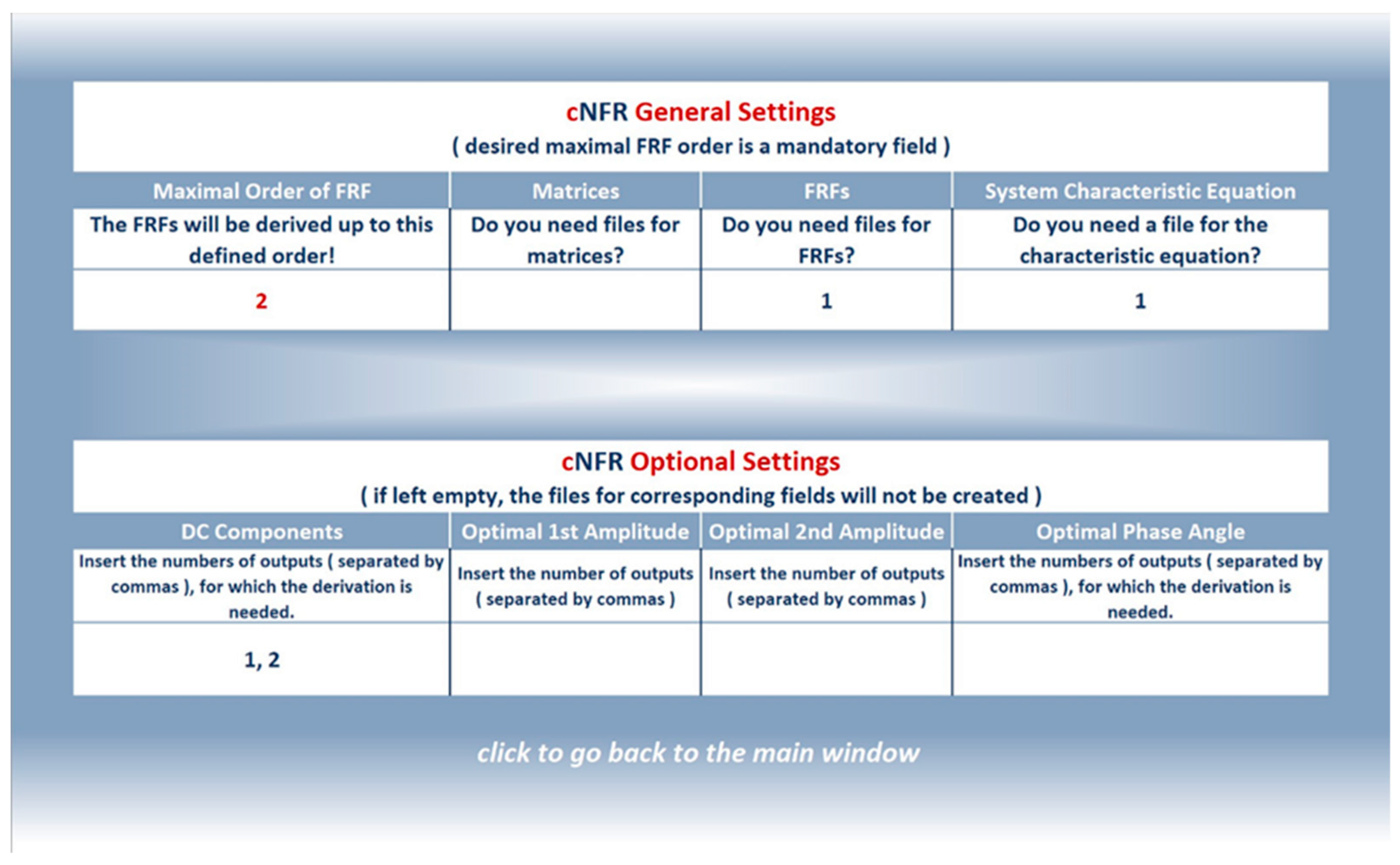
The cNFR interface also allows the user to define some additional settings, including specifications of the information to be generated by the cNFR application. In the Navigation Window, which is part of Main Window (Figure 4), the user can click on the following seven navigation buttons: (1) Order of Derivation, (2) Project Name, (3) Balance Equations (4) Inputs, (5) Outputs, (6) General Settings, and (7) Optional Settings. Clicking on these buttons will quickly navigate the user to the corresponding fields to be filled.

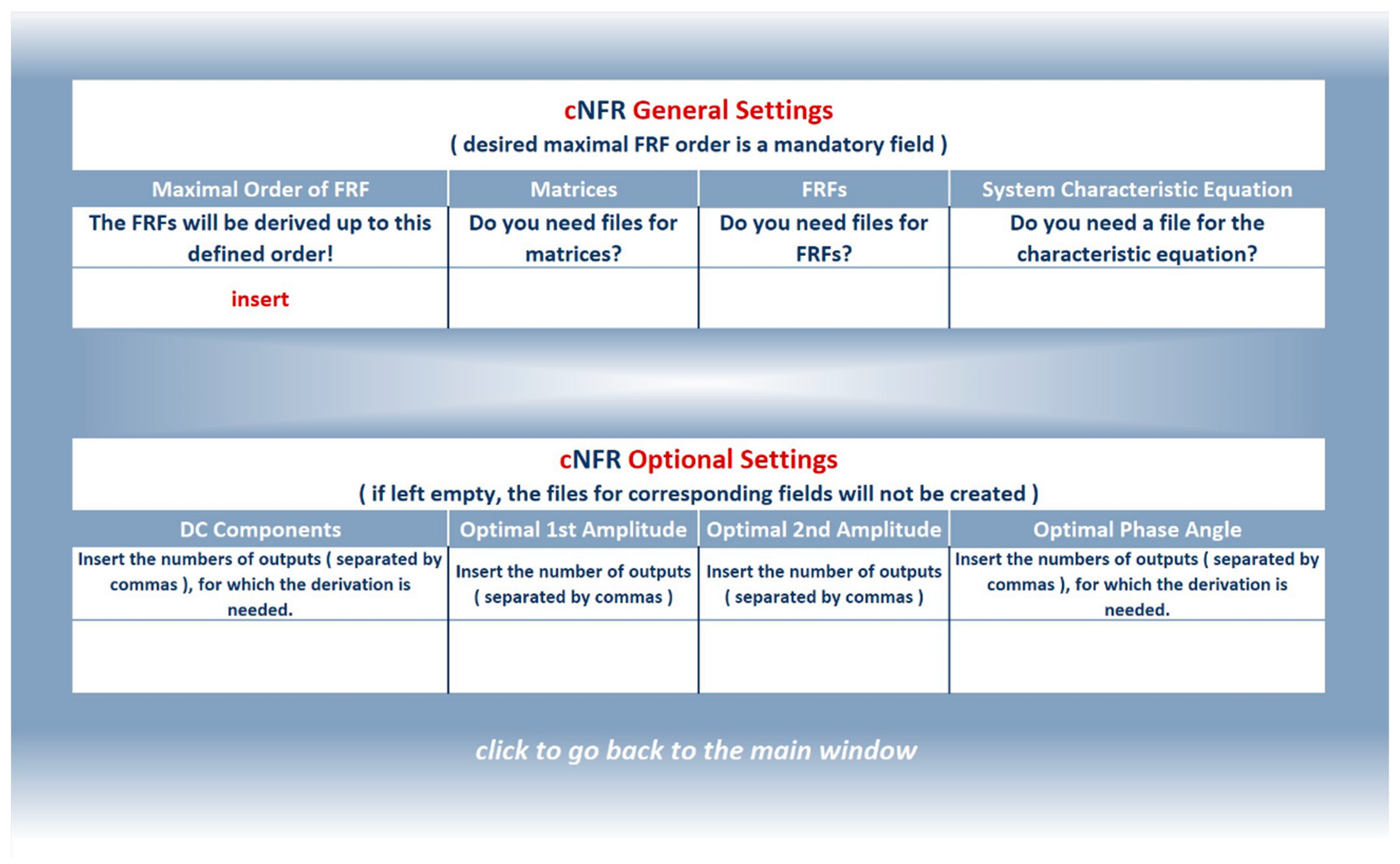
By clicking on “General and Optional Settings”, or “Order of Derivation” button, the user is transferred to the Settings Window, shown in Figure 5. In the Settings Window, the user can choose to derive the DC components and the optimal amplitudes and phase angle for the chosen output of interest. Also, the user can select whether the cNRF application will automatically generate files for matrices, FRFs, and the characteristic equation. The only mandatory field in the Settings Window is the “Maximal Order of FRF” which defines the order up to which the cNFR application will derive the FRFs.

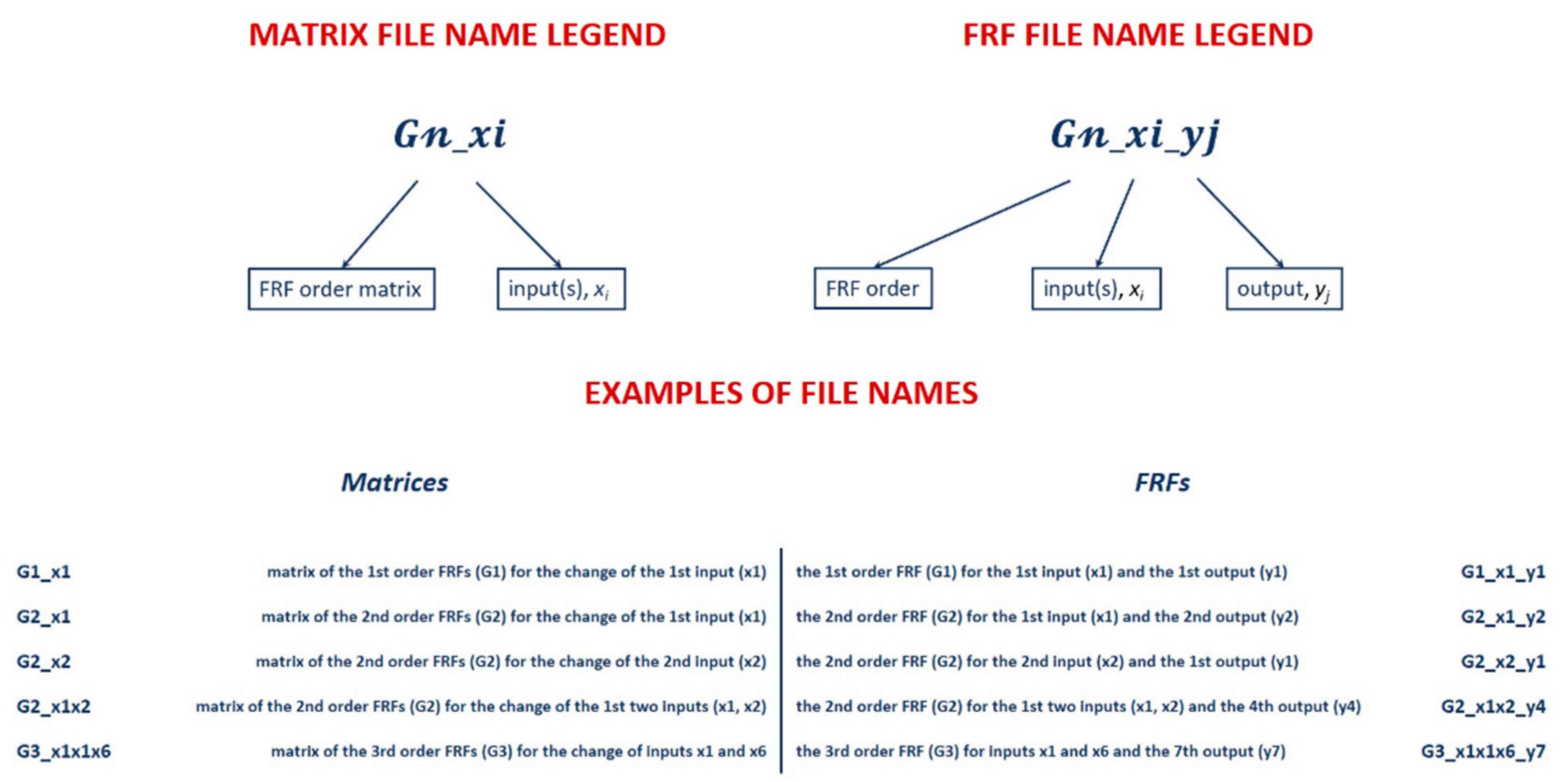
At the bottom of the Settings Window the user can see the Legend Window (Figure 6) that explains the names of the matrix and FRF files automatically generated by the cNFR application, along with some examples. The file generated for matrices contains FRFs of all outputs defined (Figure 4) and $i$-th input. E.g., matrix file name G1_xi would contain the matrix with the first-order FRFs of all outputs for modulation of the $i$-th input variable. On the other hand, FRF file names contain only one FRF for a $j$-th output and $i$-th input. In systems with a very large number of output variables, it is convenient and faster to create only files for matrices instead of $i·j$ number of files for FRFs, as all necessary FRFs can be easily withdrawn from the matrices.

After filling the necessary fields, the user can start the derivation by running the MATLAB code (step two shown in Figure 3). The code reads the user-supplied data and performs the automatic derivation of the FRFs and further computations which give insight into the system dynamics.

MATLAB Symbolic Math Toolbox is used for variable creation, the transformation of the variables into dimensionless form, Taylor series expansion, creation of the Volterra series of all outputs, symbolic substitutions, harmonic probing, solving the systems of equations, deriving the FRFs, and generating the characteristic equation (essentially for all derivation steps defined in Figure 2, Section 1). All derived functions are recorded in symbolic form, as well as in an optimized vector form through automatically generated MATLAB function files. These function files can be used for fast simulations and rapid rigorous optimizations. By simplifying the procedure shown in Figure 2 (Section 1) through automation, further computations, and simulation-ready file creation, the NFR method becomes user-friendly and easy-to-apply in a fast manner, even for complex systems.

The use of the cNFR application, its verification, and functionality will be demonstrated in two cases: (1) isothermal continuous stirred-tank reactor (CSTR) with simple reaction mechanism; and (2) electrochemical reaction (ECR) process.

3. Examples of the Application of the cNFR Method

3.1. Example 1: Analysis of Forced Periodic Operation of Isothermal Continuous Stirred-Tank Reactor with a Simple Reaction Mechanism (CSTR)

3.1.1. Problem Formulation

One of the simplest cases to which the standard Nonlinear Frequency Response (NFR) method (Section 1) was applied was an isothermal CSTR with constant volume and simple irreversible $n$-th order reaction [20,25]:

$$A\stackrel{k_r}{\to }P$$

(4)

following a simple reaction rate law:

$$r=k_r·C_A{}^n$$

(5)

The mathematical model of this reactor is defined by the material balances for the reactant $A$ and product $P$, which are described with the following ordinary differential equations:

$$0=-V·\frac{d{C}_A\left(t\right)}{dt}+F\left(t\right)·C_{Ai}\left(t\right)-F\left(t\right)·C_A\left(t\right)-V·k_r·C_A{}^n\left(t\right)$$

(6)

$$0=-V·\frac{d{C}_P\left(t\right)}{dt}-F\left(t\right)·C_P\left(t\right)+V·k_r·C_A{}^n\left(t\right)$$

(7)

where $t$ is time, $F$ is the volumetric flow rate (the inlet and outlet flow rates are equal owing to the assumption of a constant volume of the reaction mixture), $C_{Ai}$ is the reactant inlet concentration, and $C_A$ and $C_P$ are the outlet concentrations of reactant and product, respectively. $V$ is the volume of the reaction mixture, $n$ is the reaction order, and $k_r$ is the reaction rate constant.

It has to be noted that, in cases when the volumetric flow rate is modulated, for proper evaluation of the periodic operation it is necessary to consider the time-average values of the molar flow rates of the reactant and product,$M{F}_A$ and $M{F}_P$ [25,49], so the equations in which they are defined need to be added, as well:

$$0=-M{F}_A\left(t\right)+F\left(t\right)·C_A\left(t\right)$$

(8)

$$0=-M{F}_P\left(t\right)+F\left(t\right)·C_P\left(t\right)$$

(9)

3.1.2. Filling in the cNFR Interface and Generating Results

To apply the cNFR method, the user needs to perform Steps 1, 2, and 3, shown in Figure 3 (Section 2). The total number of equations is four ($N=4$), with no exponential terms ($L=0$). Two possible modulated inputs are considered: inlet reactant concentration, $C_{Ai}$ (input 1) and volumetric flow rate, $F$ (input 2), which can be modulated separately or simultaneously (Figure 7).

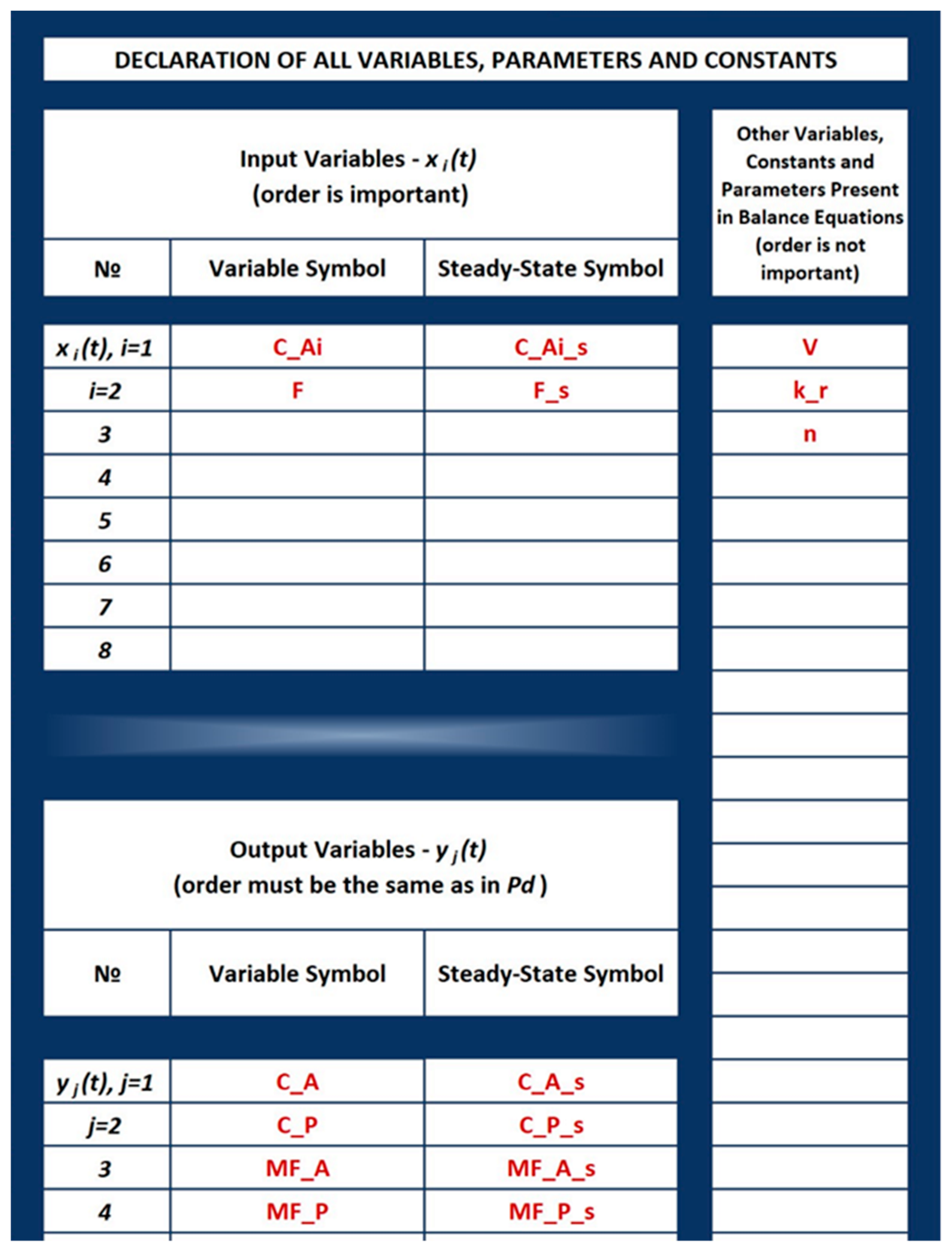
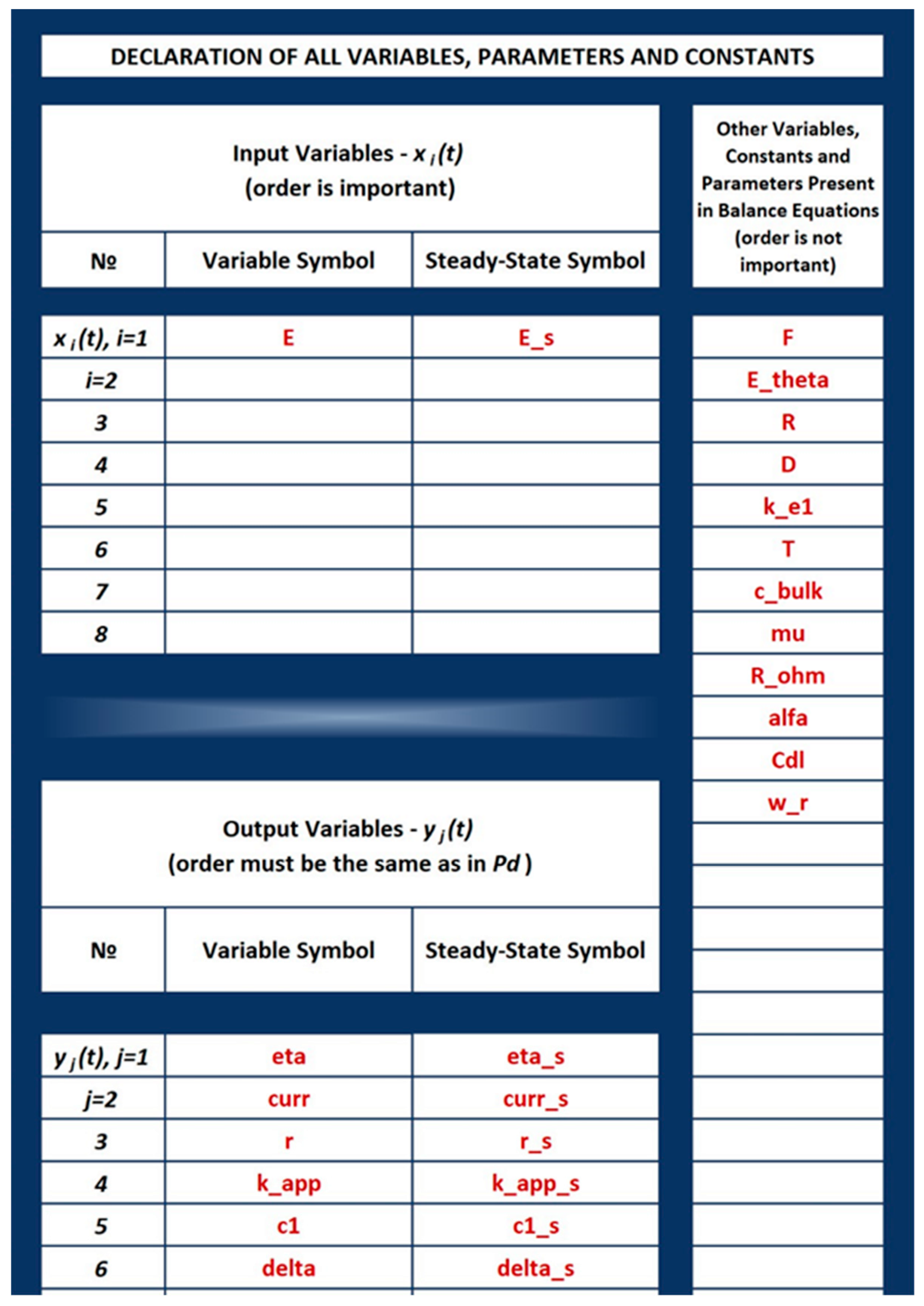
Output variables defined by the dynamic model Equations (6)–(9) are: $C_A$, $C_P$, $M{F}_A$, and $M{F}_P$. The input and output variables, their steady-state symbols, and other constants from Equations (6)–(9) are declared in the Main Window of the cNFR application, as shown in Figure 7.

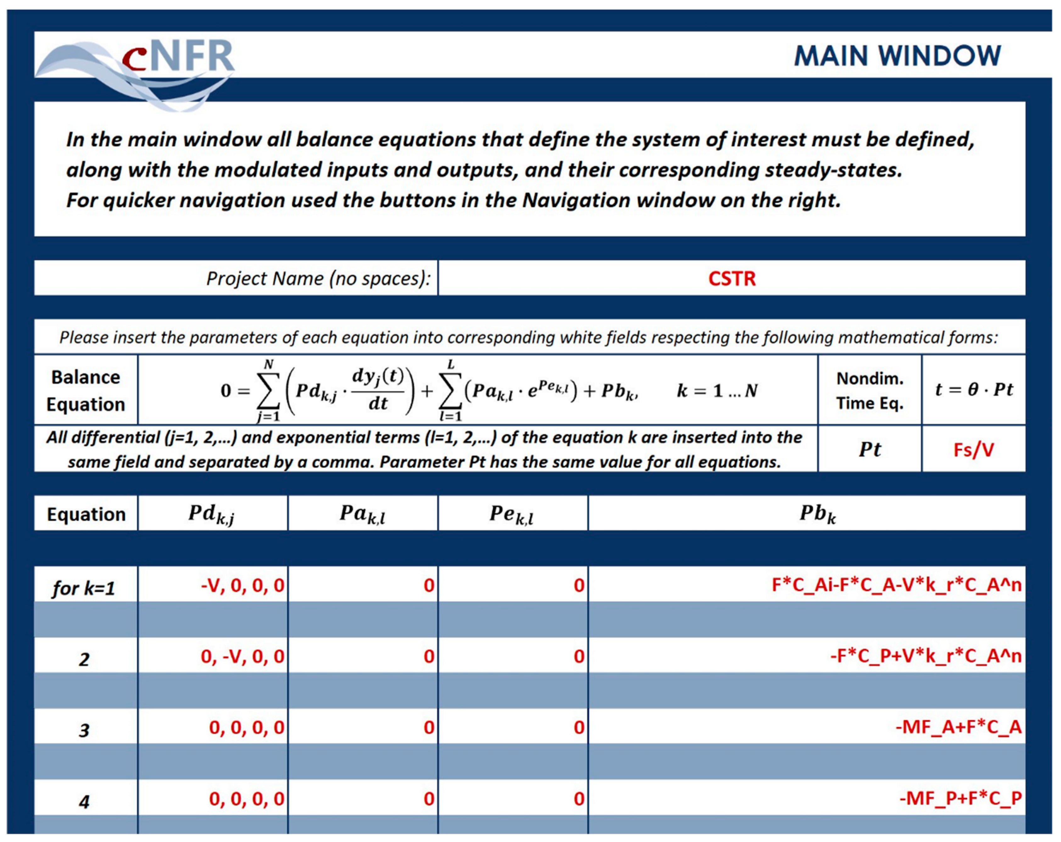
Equations (6)–(9) are written in a form which facilitates quick identification of parameters $P{d}_{k,j}$, $P{a}_{k,l}$, $P{e}_{k,l}$, and $P{b}_k$ for each equation, $k$, of the dynamic model. These parameters practically define the model equations in the form of Equation (2), which is also shown in the Main Window of the cNFR application (Figure 4, Section 2).

Like in the work by Nikolic Paunic and Petkovska [25], nondimensional time is used, defined as a ratio of the dimensional time $t$ and the reactor residence time. Accordingly, the parameter $Pt$ Equation (3) (Section 2) is defined as a reciprocal value of the steady-state residence time (Figure 8):

$$Pt=\raisebox{1ex}{$F_s$}\!\left/ \!\raisebox{-1ex}{$V$}\right.$$

(10)

As a result of Equation (10), the frequency of input change, ${\omega }_{nd}$, will also be nondimensional. Considering the order of the declared output variables: $C_A$, $C_P$, $M{F}_A$, $M{F}_P$, the $Pd$ parameters corresponding to the differential terms in the first equation Equation (6) are:

$$P{d}_{1,1\dots 4}=\left[-V, 0, 0, 0\right]$$

(11)

In Equation (6), there are no exponential terms, so the parameters $P{a}_1$ and $P{e}_1$ are zero:

$$P{a}_1=P{e}_1=0$$

(12)

The remaining terms in Equation (6) represent the parameter $P{b}_1$:

$$P{b}_1=F·C_{Ai}-F·C_A-V·k_r·C_A{}^n$$

(13)

Analogously, the parameters corresponding to Equation (7) are defined in the following way:

$$P{d}_{2,1\dots 4}=\left[0, -V, 0, 0\right]$$

(14)

$$P{a}_2=P{e}_2=0$$

(15)

$$P{b}_2=-F·C_P+V·k_r·C_A{}^n$$

(16)

Equations (8) and (9) have no differential or exponential terms so their parameters are defined as:

$$P{d}_{3,1\dots 4}=\left[0,0,0,0\right]$$

(17)

$$P{a}_3=P{e}_3=0$$

(18)

$$P{b}_3=-M{F}_A+F·C_A$$

(19)

$$P{d}_{4,1\dots 4}=\left[0, 0, 0, 0\right]$$

(20)

$$P{a}_4=P{e}_4=0$$

(21)

$$P{b}_4=-M{F}_P+F·C_P$$

(22)

The Main Window in which the parameters defined in Equations (10)–(22) have been inserted is shown in Figure 8.

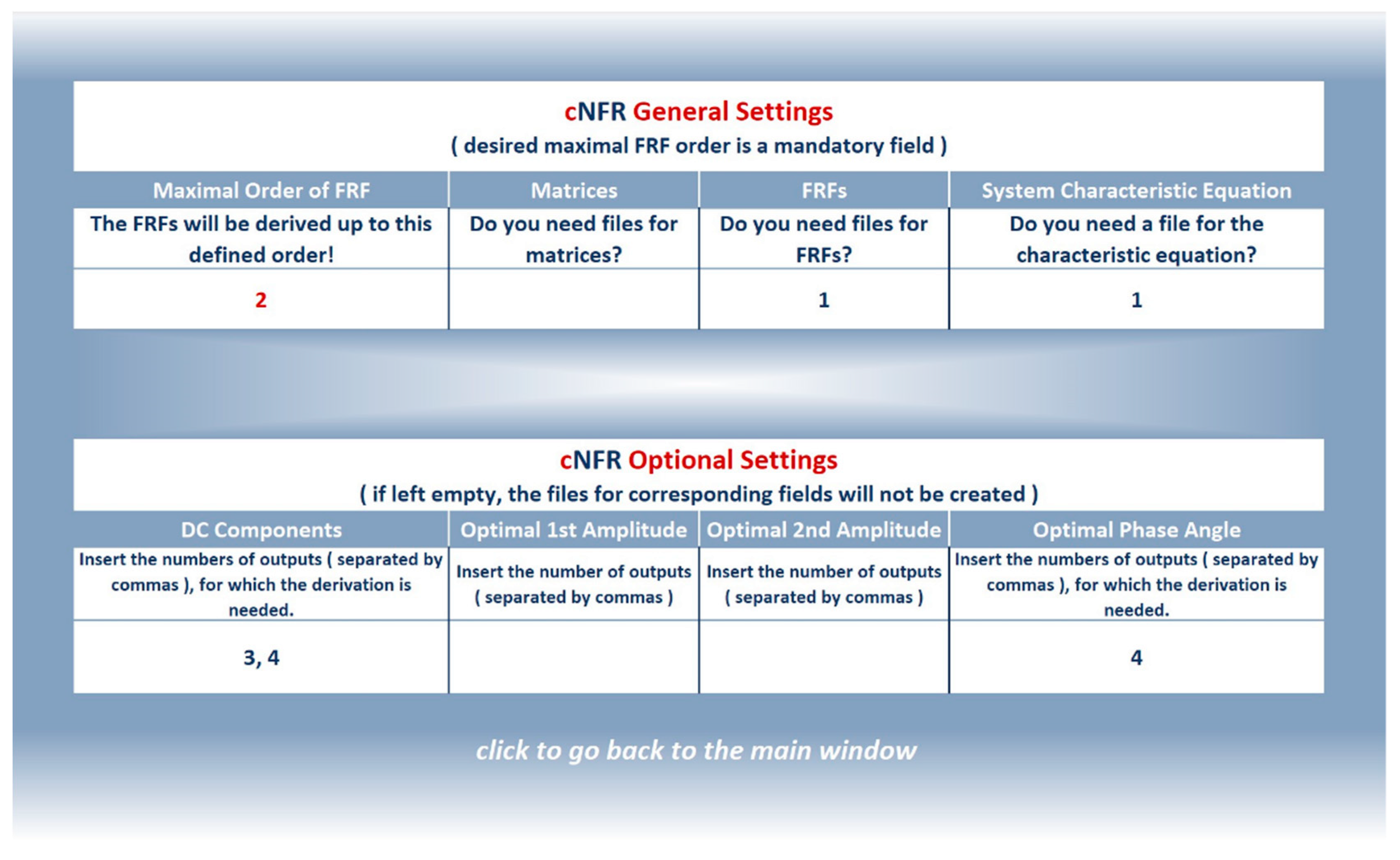
The FRFs are derived up to the second order (Figure 9), and the files that are automatically generated by the cNFR application are: (1) all FRFs (for theoretical verification of the cNFR method), (2) characteristic equation (for stability analysis), (3) the DC components of the molar flow rates, and (4) the optimal phase angle maximizing the fourth output variable, $y_4$, i.e., the molar flow rate of the product, $M{F}_P$ (for analyzing the forced periodic operation).

After filling the Project Name field in the cNFR Main Window (Figure 8), the user starts the second stage of the cNFR routine (Figure 3) by running the MATLAB code and inserting the name of the project Excel worksheet. When the program has finished running, the user obtains a folder created by the cNFR application. The folder bears the name of the project specified by the user in the Main Window (Figure 8). For Example 1, a folder named “CSTR” is created, which contains the function files for the first and second-order FRFs and the DC components for the outlet molar flow rates for three different scenarios: (1) single-input modulation of the reactant concentration; (2) single-input modulation of the volumetric flow rate, and (3) simultaneous modulation of the reactant concentration and volumetric flow rate. The names of the FRF files are generated using the principle shown in the Legend Window in Figure 6 (e.g., G1_x1_y4 is the first-order FRF for the product outlet molar flow rate when reactant inlet concentration is modulated). The DC component files will start with letters ‘DC’ (e.g., DC_x1x2_y4 is the DC component for the product outlet molar flow rate when both reactant inlet concentration and volumetric flow rate are modulated), while the optimal phase angle file will be present in the folder under the name ‘OPT_FI’. The cNFR application also leaves a “.mat” file that contains all derived analytical formulas in its symbolic form and informs the user about the time needed for the computation to be completed. For Example 1, the computation time was only 51.3 s.

3.1.3. Simulating the FRFs Derived Using cNFR and its Verification

The FRFs derived using the cNFR application are theoretical analytical functions. However, they are not obtained in their most concise or elegant form and can seem quite cumbersome at first sight. That is the reason why they are not presented here. Nevertheless, by setting the values of the model parameters and the frequency range, they can be used for simulation of the FRFs and DC components of interest.

The software application for the cNFR method was first verified by comparing the automatically derived FRFs with the same functions derived using the classical approach [49]. The asymmetrical second-order FRFs corresponding to the outlet molar flow-rates of the product were chosen for comparison. Their analytical expressions from the literature [49] are:

• For modulation of the inlet reaction concentration, $C_{Ai}$ (input $x_1$):

  $$G_{x1,y4}^{\left(2\right)}\left({\omega }_{nd},-{\omega }_{nd}\right)=\frac{{\left(1+\alpha \right)}^2}{2·B_{ps}}·\frac{n·\left(n-1\right)}{{\omega }_{nd}{}^2+B_{ps}{}^2}$$

  (23)
• For modulation of the volumetric flow rate, $F$ (input $x_2$):

  $$G_{x2,y4}^{\left(2\right)}\left({\omega }_{nd},-{\omega }_{nd}\right)=\frac{1}{2·B_{ps}}·\frac{n·\left(n-1\right)·{\alpha }^2+2·n·\alpha ·\left(1+n·\alpha \right)}{{\omega }_{nd}{}^2+B_{ps}{}^2}$$

  (24)
• The cross-function:

  $$G_{x1x2,y4}^{\left(2\right)}\left({\omega }_{nd},-{\omega }_{nd}\right)=\frac{n·\left(1+\alpha \right)}{B_{ps}}·\frac{{\omega }_{nd}{}^2+{\left(1+n·\alpha \right)}^2-\left(\alpha +1\right)+j·{\omega }_{nd}}{{\omega }_{nd}{}^2+B_{ps}{}^2}$$

  (25)

In Equations (23)–(25), two auxiliary dimensionless parameters, $\alpha$ and $B_{ps}$, have been introduced [49]:

$$\alpha =k·C_{A,s}{}^{n-1}·\frac{V}{F_s}$$

(26)

$$B_{ps}=1+n·\alpha$$

(27)

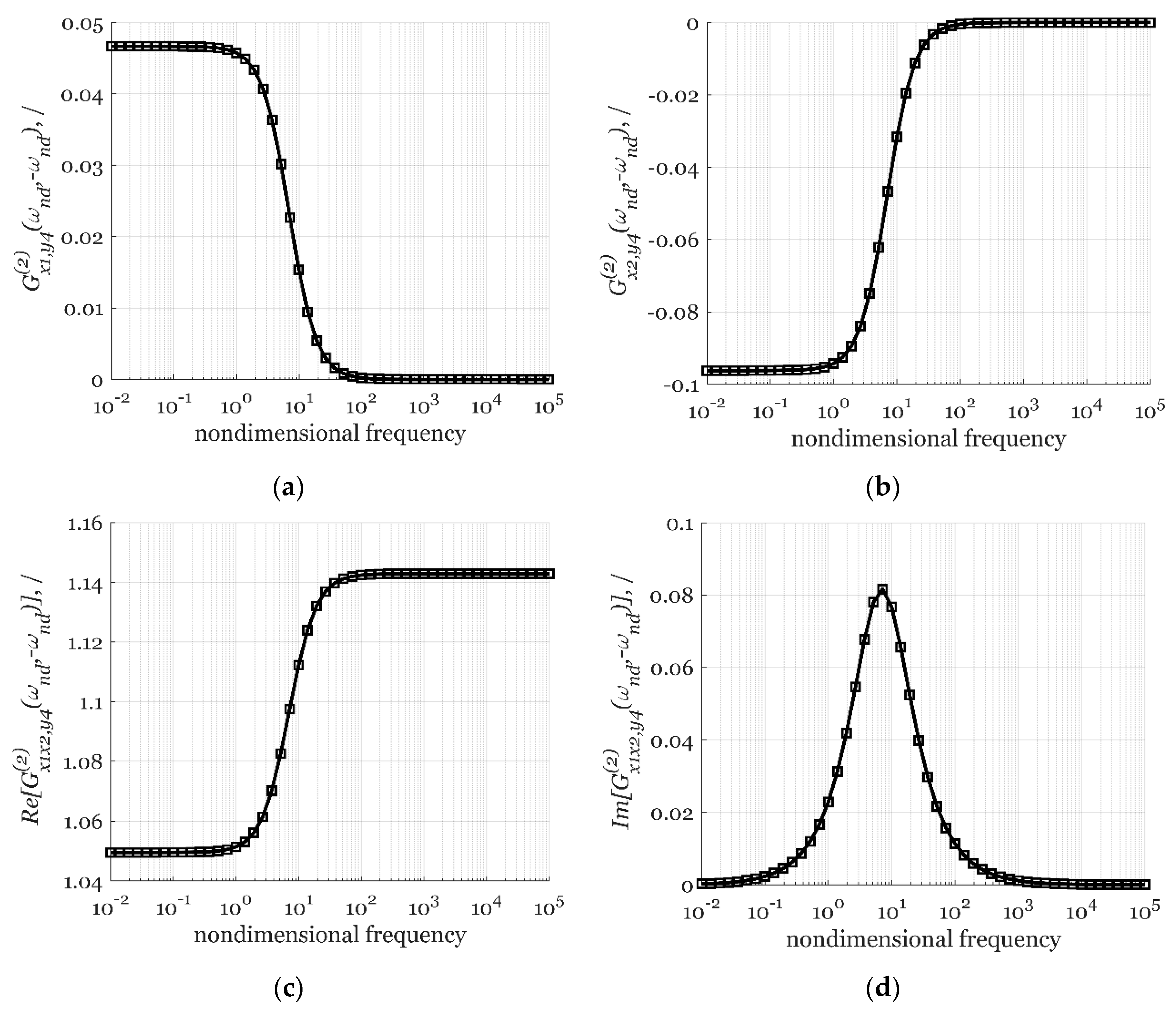
All three asymmetrical second-order FRFs corresponding to the outlet molar flow rate of the product were simulated using Equations (23)–(27) and the automatically derived functions using the cNFR application, with parameter and constant values given in

Table 1. Values of parameters and constants used for simulation in Example 1: CSTR.

Label	Units	Value
$C_{Ai,s}$	kmol/m3	16.02
$F_s$	m3/min	0.0472
$V$	m3	28.32
$k_r$	m3/kmol/min	1.248
$n$	/	2
$A_1$	/	0.9
$A_2$	/	0.9

[49]. As shown in Figure 10, the FRFs simulated using the results of the cNFR application and Equations (23)–(27) are identical.

3.1.4. Analyzing System Stability

From the simulated FRFs, the user can analyze the dynamics of the system in the desired frequency range, for any set of operational parameters. However, the NFR method is applicable only if the system is stable. Therefore, the cNFR application also generates an algebraic and vector form of the system characteristic equation. The system will be stable only if the roots of the characteristic equation are negative or have negative real parts (if they are complex numbers). This is especially important while estimating system parameters or optimizing operational values, as the roots of the characteristic equation can be used as algebraic constraints. In Example 1, the cNFR generated characteristic equation is:

$$C_{A,s}·F_s·s^2+\left(n·k_r·C_{A,s}{}^n·V+2·C_{A,s}·F_s\right)·s+n·k_r·C_{A,s}{}^n·V+C_{A,s}·F_s=0$$

(28)

Therefore, the roots of the characteristic equation must satisfy the following condition:

$$-C_{A,s}·F_s-C_{A,s}{}^n·V·k_r·n<0$$

(29)

i.e.,

$$1+n·V·k_r·C_{A,s}{}^{n-1}>0$$

(30)

which is identical to the stability condition for this example reported previously by Nikolic Paunic [49].

3.1.5. Analyzing System Forced Periodic Operation

As explained shortly in Section 1 and extensively documented in our previous publications [44,49], the NFR analysis offers an easy way to evaluate the potential of intensification of an operation which is classically performed in a steady state by forced periodic modulation of one or more inputs around their steady-state values. If we refer to Figure 1 (Section 1), the intensification is directly related to the DC component of the output of interest, which can be approximately evaluated using only the asymmetrical second-order FRFs and the input parameters.

For a simultaneous co-sinusoidal modulation of the feed concentration $C_{Ai}$ and flow rate $F$, around their steady-state values $C_{Ai,s}$ and $F_s$, with amplitudes $A_1$ and $A_2$, frequency $\omega$, and phase shift $\phi$, defined as:

$$C_{Ai}\left(t\right)=C_{Ai,s}·\left[1+A_1·\cos \left(\omega ·t\right)\right]$$

(31)

$$F\left(t\right)=F_s·\left[1+A_2·\cos \left(\omega ·t+\phi \right)\right]$$

(32)

the DC component can be approximately obtained as [25,49]:

$$\begin{array}{c}D{C}_{x1x2,y4}\approx 2·{\left(\frac{A_1}{2}\right)}^2·G_{x1,y4}^{\left(2\right)}\left(\omega ,-\omega \right)+2·{\left(\frac{A_2}{2}\right)}^2·G_{x2,y4}^{\left(2\right)}\left(\omega ,-\omega \right)+\\ 2·\left(\frac{A_1}{2}\right)·\left(\frac{A_2}{2}\right)·\left\{cos\left(\phi \right)·Re\left[G_{x1x2,y4}^{\left(2\right)}\left(\omega ,-\omega \right)\right]+sin\left(\phi \right)·Im\left[G_{x1x2,y4}^{\left(2\right)}\left(\omega ,-\omega \right)\right]\right\}\end{array}$$

(33)

The optimal phase difference between the modulated inputs, maximizing the cross effect and, accordingly the DC component, is evaluated from the cross asymmetrical second-order FRF [25,49]:

$${\phi }_{opt}\left(\omega \right)=arctan\left\{\frac{Im\left[G_{x1x2,y4}^{\left(2\right)}\left(\omega ,-\omega \right)\right]}{Re\left[G_{x1x2,y4}^{\left(2\right)}\left(\omega ,-\omega \right)\right]}\right\}$$

(34)

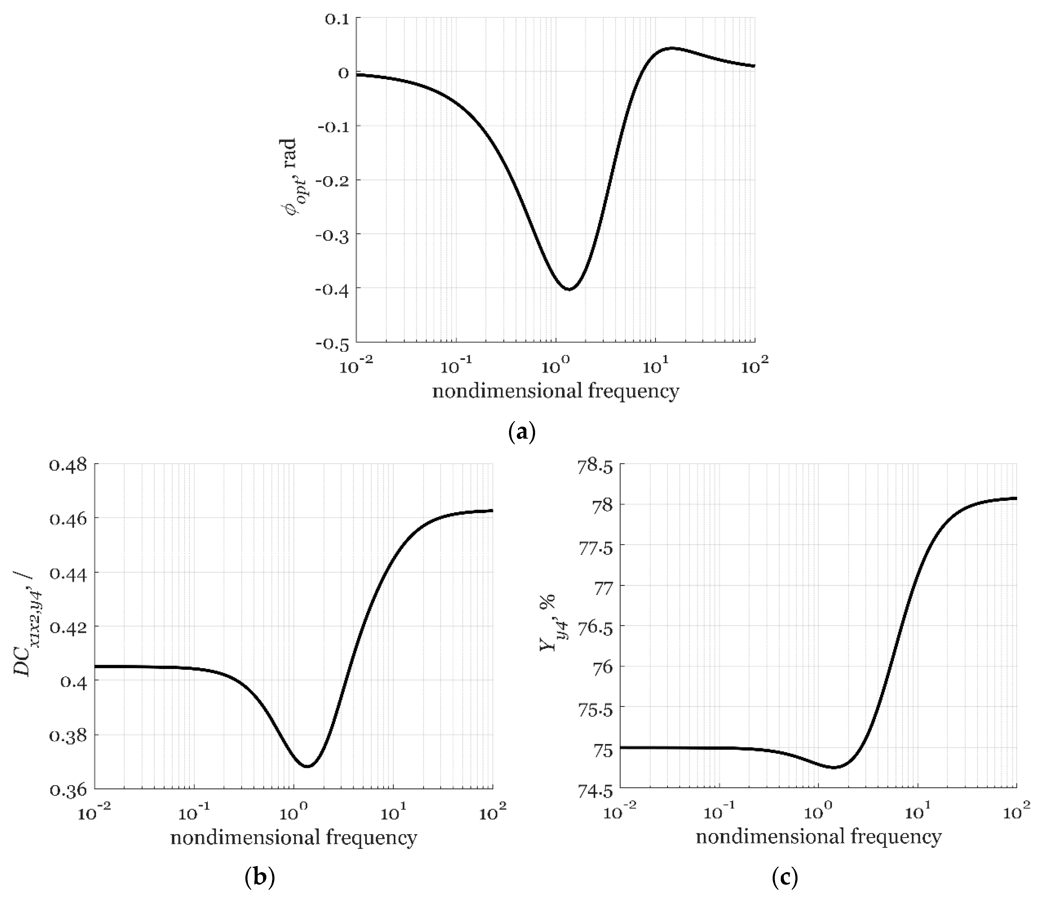
Figure 11b shows the DC component corresponding to the outlet molar flow rate of the product $M{F}_P$ in a wide frequency range, calculated using the parameters given in Table 1 and the optimal phase difference, shown in Figure 11a. As shown in Figure 11b, the highest values of $D{C}_{x1x2,y4}$, i.e., an increase of $M{F}_P$, is predicted in the high-frequency range where the corresponding optimal phase angle will be 0 rad (both inputs are modulated in-phase).

This analysis can be further extended to investigating the product yield corresponding to the periodic operation, which can be easily evaluated from the DC component of the outlet molar flow rate [48,49]:

$$Y_{y4}=\frac{\overline{M{F}_P}}{\overline{F·C_{Ai}}}=\frac{M{F}_{P,s}}{F_s·C_{Ai,s}}·\frac{\left(1+D{C}_{x1x2,y4}\right)}{1+2·\frac{A_1}{2}·\frac{A_2}{2}·\cos \left(\phi \right)}$$

(35)

The product yield simulation results are shown in Figure 11c and they show that the highest product yield is also achieved in the high-frequency range.

3.2. Example 2: Analysis of an Electrochemical Reaction Process (ECR)—Comparison with Experimental Results

3.2.1. Problem Formulation

The cNFR application will also be illustrated in the case of electrochemical oxygen reduction reaction (ORR) on a rotating disc electrode, for which the NFR method was applied experimentally [39]. The FRFs derived using the cNFR method will be compared to the ones estimated from the experimental measurements.

The ORR single-step mechanism can be written as [39]:

$$O_2+e^{-}\stackrel{k_{app}}{\to }products$$

(36)

In this study, we use the mathematical model for the single-step ORR mechanism from Kandaswamy et al. [39]. All model equations are written in the standard form defined by Equation (2) (Section 2).

The electrical charge balance can be written as:

$$0=-c_{dl}·\frac{d\eta \left(t\right)}{dt}+curr\left(t\right)+F·4·r\left(t\right)$$

(37)

where $c_{dl}$ is the double-layer capacitance, $\eta$ the electrode overpotential, $F$ the Faraday’s constant, $r$ the ORR reaction rate expression, and $curr$ the current density, which is the main output of interest.

The potential balance is:

$$0=-\eta \left(t\right)+E\left(t\right)-E^{\theta }-R_{\mathsf{\Omega }}·curr\left(t\right)$$

(38)

where $E$ is the electrode potential, which is a possible modulated input, while $E^{\theta }$ is the standard electrode potential, and $R_{\mathsf{\Omega }}$ ohmic resistance.

The kinetics of the ORR is described by the following reaction rate expression:

$$0=-r\left(t\right)+k_{app}\left(t\right)·\frac{c_1\left(t\right)}{1+\frac{k_{app}\left(t\right)}{D/\left(\delta \left(t\right)/2\right)}}$$

(39)

where $k_{app}$ is the apparent rate constant of the ORR, which is a function of overpotential and temperature, defined by the equation:

$$0=-k_{app}\left(t\right)+k_{e1}·e^{-\frac{\alpha ·F}{R·T}·\eta \left(t\right)}$$

(40)

$k_{e1}$ is the ORR kinetic constant, $\alpha$ the transfer coefficient, $R$ the universal gas constant, and $T$ the reaction temperature, which is assumed to be constant in our current analysis.

In Equation (39) $c_1$ is the intermediary oxygen concentration derived from the discretized mass balance equation [39]:

$$0=-\frac{d{c}_1\left(t\right)}{dt}+\frac{D}{\delta {\left(t\right)}^2/2}·\left(c_{bulk}-c_1\left(t\right)\right)-\frac{D}{\delta {\left(t\right)}^2/2}·\frac{c_1\left(t\right)·k_{app}\left(t\right)}{D/\delta \left(t\right)+k_{app}\left(t\right)}$$

(41)

where $\delta$ is the electrode boundary layer thickness and depends on the electrode rotation rate ${\omega }_r$ and some physical parameters (the oxygen diffusivity in the boundary layer, $D$, and the kinematic viscosity of the NaOH solution in which the reaction takes place, $\nu$) according to the equation:

$$0=-\delta \left(t\right)+1.61·D^{\frac{1}{3}}·{\nu }^{\frac{1}{6}}·{\omega }_r{\left(t\right)}^{-\frac{1}{2}}$$

(42)

3.2.2. Filling in the cNFR Interface and Generating Results

In the current study, only one input is considered - the electrode potential E, which was used as the modulated input in the experimental study by Kandaswamy et al. [39]. In principle, other inputs could also be used, e.g., the electrode rotation rate or the bulk concentration.

The input, and well as its steady-state symbol ($E_s$) are declared in the Main Window of the cNFR application, as shown in Figure 12.

There is a total of six dynamic model equations (Equations (37)–(42)) and six possible outputs ($\eta$,$curr$, $k_{app}$, $r$, $c_1$, and $\delta$), so $N=6$. Our main output of interest is the current density $curr$ (output $y_2$). Only Equation (40) has one exponential term, so $L=1$. For an easier comparison of the experimental and cNFR generated FRFs, dimensional time was used ($Pt=1$). Equations (37)–(42) are written in a way to quickly identify parameters $P{d}_k$-$P{b}_k$ for all six equations ($N=6$). Considering the sequence of the model Equations (37)–(42) and the sequence of the outputs ($\eta$,$curr$, $k_{app}$, $r$, $c_1$, and $\delta$), these parameters are defined in the following way:

$$P{d}_{1,1\dots 6}=\left[-c_{dl}, 0, 0, 0,0,0\right]$$

(43)

$$P{a}_1=P{e}_1=0$$

(44)

$$P{b}_1=curr\left(t\right)+F·4·r\left(t\right)$$

(45)

$$P{d}_{2,1\dots 6}=0$$

(46)

$$P{a}_2=P{e}_2=0$$

(47)

$$P{b}_2=-\eta \left(t\right)+E\left(t\right)-E^{\theta }-R_{\mathsf{\Omega }}·curr\left(t\right)$$

(48)

$$P{d}_{3,1\dots 6}=0$$

(49)

$$P{a}_3=P{e}_3=0$$

(50)

$$P{b}_3=-r\left(t\right)+k_{app}\left(t\right)·\frac{c_1\left(t\right)}{1+\frac{k_{app}\left(t\right)}{D/\left(\delta \left(t\right)/2\right)}}$$

(51)

$$P{d}_{4,1\dots 6}=0$$

(52)

$$P{a}_4=-k_{e1}\left(t\right)$$

(53)

$$P{e}_4=-\frac{\alpha ·F}{R·T}·\eta \left(t\right)$$

(54)

$$P{b}_4=-k_{app}\left(t\right)$$

(55)

$$P{d}_{5,1\dots 6}=\left[0, 0, 0, 0,-1,0\right]$$

(56)

$$P{a}_5=P{e}_5=0$$

(57)

$$P{b}_5=\frac{D}{\delta {\left(t\right)}^2/2}·\left(c_{bulk}-c_1\left(t\right)\right)-\frac{D}{\delta {\left(t\right)}^2/2}·\frac{c_1\left(t\right)·k_{app}\left(t\right)}{D/\delta \left(t\right)+k_{app}\left(t\right)}$$

(58)

$$P{d}_{6,1\dots 6}=0$$

(59)

$$P{a}_6=P{e}_6=0$$

(60)

$$P{b}_6=-\delta \left(t\right)+1.61·D^{\frac{1}{3}}·{\nu }^{\frac{1}{6}}·{\omega }_r{\left(t\right)}^{-\frac{1}{2}}$$

(61)

The parameters $P{d}_k$-$P{b}_k$ are then inserted into the corresponding fields of the cNFR Main Window, shown in Figure 13.

In the cNFR Settings Window (Figure 14), it was chosen that files are generated for the FRFs up to the second order.

For Example 2, the cNFR method computational time was 64 s.

3.2.3. Comparison with Experimental FRFs and Model Identification

The experimental FRFs can be directly estimated from the harmonics and the DC component of the measured output, obtained in the experimental frequency response measurements, as shown in Figure 1 (Section 1). In our previous study [39] the harmonics of the NFR were measured using a Solartron Energy Lab XM potentiostat made by Ametek. From the measurements, the first-order and the symmetrical second-order FRFs were estimated.

The files generated using the cNFR application contain the analytical expressions of the theoretical first and second-order FRFs corresponding to the model defined in Section 3.2.1. Due to their rather cumbersome form, the analytical expressions of the derived theoretical FRFs are not given here but can be found in the Supplementary Material of Kandaswamy et al. [39].

The generated function files allow fast and easy simulation of the FRFs for any set of parameter values. They were simulated for the experimental conditions used in the experimental investigation [39], for two different cases with vastly different electrolyte concentration in the electrochemical reaction (0.1 M and 11 M NaOH solution). The values of the constants and parameters used for simulation are given in

Table 2. Values of parameters and constants used for simulation in Example 2: ECR.

Label	Units	Value in 0.1 M NaOH	Value in 11 M NaOH
$c_{bulk}$	mol/m3	1.18	0.05
$c_{dl}$	F/m2	1.15	1.40
$D$	m2/s	1.9 × 10−9	6.0 × 10−11
$k_{e1}$	m/s	4.7 × 10−9	5.5 × 10−10
$E^{\theta }$	V	1.222	1.171
$\nu$	m2/s	1.0128 × 10−6	1.2800 × 10−5
$R_{\mathsf{\Omega }}$	Ω m2	9.731 × 10−4	1.111 × 10−4
$\alpha$	/	0.445	0.500
$E_s$	V	0.9
${\omega }_r$	rpm	1600
$T$	K	293.15
$F$	C/mol	96485
$R$	J/mol/K	8.314

.

The comparison of the experimental and theoretical FRFs derived using the cNFR application, relating the current density as the output of interest and the potential, is shown in Figure 15. For easier comparison with the experimentally estimated functions, the FRFs are given in their dimensional form. The derived first-order FRF results can be seen in Figure 15a (amplitude) and 15b (phase), and the symmetrical second-order FRF in Figure 15c (amplitude) and 15d (phase).

The results, shown in Figure 15a,b, correspond to the admittance of the Electrochemical Impedance Spectroscopy (EIS). For both cases (0.1 and 11 M NaOH solution) excellent agreement between the experimental and simulated amplitudes and phases for the first-order FRFs (admittance) is obtained. Therefore, EIS, which focuses on the linear part of the response, would suggest that the mathematical model given in Section 3.2.1 successfully describes the ORR reaction, both for low and high concentrations of NaOH.

On the other hand, by comparing the experimental and theoretical symmetrical second-order FRFs, it is obvious that good agreement is obtained only for the case of diluted solution (0.1 M NaOH) for low and moderate frequencies, while the agreement for the case of concentrated solution (11 M NaOH) is poor. The discrepancies between the experimental and theoretical symmetrical second-order FRFs (corresponding to the nonlinear part of the response), which are distinctive for the 11 M solution, could be a result of some phenomena that were not mathematically described by the single-step mechanism (Equations (37)–(42), Section 3.2.1) used for deriving the theoretical FRFs. This result is a strong indication that a more complex several-step mechanism of the ORR system should be considered and used for deriving the theoretical FRFs. By using the cNFR application, this should be a rather simple and easy task.

4. Conclusions

The computer-aided Nonlinear Frequency Response (cNFR) method, presented in this paper, is an important upgrade of the Nonlinear Frequency Response method developed and used in our research group over the last two decades. It uses an original software application for automatic derivation of theoretical frequency response functions (FRFs) that are a very convenient and useful way of mathematically representing the dynamics of nonlinear systems. The automation of the derivation process facilitates the use of the NFR method substantially and will, hopefully, encourage other researchers and engineers to use it more extensively.

The cNFR application uses an Excel-based interface for defining the model equations, inputs, and outputs of the investigated system and a MATLAB code that performs the symbolic mathematical derivations. As a result, the cNFR application generates MATLAB function files containing the derived FRFs in a symbolic form, which can be used for simulation, analysis, experimental identification, and process optimization. Although the derivation procedure underlying this application is rather complex, the application itself is user-friendly and requires only the basic knowledge of Excel and MATLAB.

The automatic derivation of the FRFs is just the first step in the process of full automation of the NFR method. One direction of this automation, related to developing of new experimental techniques and sophisticated software instruments, would assume integration of the current cNFR application with an automated system for running the frequency response measurements, collecting and analyzing data, estimation of the experimental FRFs, mechanism discrimination, and model identification based on comparison of the experimental and theoretical FRFs and parameter estimation. Another direction, related to the development and optimization of periodic processes, would assume integration of the cNFR application with multi-objective optimization tools.

The presented cNFR application is a prerequisite for any further advancements in both directions.

References

- Kramers, H.; Alberda, G. Frequency response analysis of continuous flow systems. Chem. Eng. Sci. 1953, 2, 173–181. [Google Scholar] [CrossRef]
- Deisler, P.F.; Wilhelm, R.H. Diffusion in beds of porous solids. Measurement by frequency response techniques. Ind. Eng. Chem. 1953, 45, 1219–1227. [Google Scholar]
- Turner, G.A. The frequency response of some illustrative models of porous media: Experiments and computations with two artificial packed beds to illustrate a method of determining parameters of the bed. Chem. Eng. Sci. 1959, 10, 14–21. [Google Scholar] [CrossRef]
- Ritter, A.B.; Douglas, J.M. Frequency response of nonlinear systems. Ind. Eng. Chem. Fundam. 1970, 9, 21–28. [Google Scholar] [CrossRef]
- Gray, R.I.; Prados, J.W. The dynamics of a packed gas absorber by frequency response analysis. AIChE J. 1963, 9, 211–216. [Google Scholar] [CrossRef]
- Devereux, B.M.; Denn, M.M. Frequency response analysis of polymer melt spinning. Ind. Eng. Chem. Res. 1994, 33, 2384–2390. [Google Scholar] [CrossRef]
- Mehta, S.C.; Shemilt, L.W. Frequency response of liquid fluidized systems. Part ii effect of liquid viscosity. Can. J. Chem. Eng. 1976, 54, 43–51. [Google Scholar]
- Stephanopoulos, G. Chemical Process Control—An Introduction to Theory and Practice; Prentice Hall: Inglewood Cliffs, NJ, USA, 1980. [Google Scholar]
- Weiner, D.D.; Spina, J.F. Sinusoidal Analysis and Modeling of Weakly Nonlinear Circuits; Van Nostrand: New York, NY, USA, 1980. [Google Scholar]
- Volterra, V. Theory of Functionals and of Integral and Integro-Differential Equations; Dover: New York, NY, USA, 1959. [Google Scholar]
- Bracewell, R.N. The Fourier Transform and Its Applications; McGraw-Hill: New York, NY, USA, 1986. [Google Scholar]
- Chatterjee, A.; Vyas, N.S. Convergence analysis of volterra series response of nonlinear systems subjected to harmonic excitation. J. Sound Vib. 2000, 236, 339–358. [Google Scholar] [CrossRef] [Green Version]
- Edwards, W.M.; Kim, H.N. Multiple Steady States in FCC Unit Operations. In Tenth International Symposium on Chemical Reaction Engineering; Pergamon: Oxford, UK, 1988; pp. 1825–1830. [Google Scholar]
- Petkovska, M.; Do, D.D. Nonlinear frequency response of adsorption systems: Isothermal batch and continuous flow adsorbers. Chem. Eng. Sci. 1998, 53, 3081–3097. [Google Scholar] [CrossRef]
- Petkovska, M.; Do, D.D. Use of higher-order frequency response functions for identification of nonlinear adsorption kinetics: Single mechanisms under isothermal conditions. Nonlinear Dyn. 2000, 21, 353–376. [Google Scholar] [CrossRef]
- Petkovska, M.; Petkovska, L.T. Use of nonlinear frequency response for discriminating adsorption kinetics mechanisms resulting with bimodal characteristic functions. Adsorption 2003, 9, 133–142. [Google Scholar] [CrossRef]
- Petkovska, M.; Seidel-Morgenstern, A. Nonlinear frequency response of a chromatographic column. Part i: Application to estimation of adsorption isotherms with inflection points. Chem. Eng. Commun. 2005, 192, 1300–1333. [Google Scholar]
- Petkovska, M.; Marković, A. Fast estimation of quasi-steady states of cyclic nonlinear processes based on higher-order frequency response functions. Case study: Cyclic operation of an adsorption column. Ind. Eng. Chem. Res. 2006, 45, 266–291. [Google Scholar]
- Petkovska, M. Nonlinear fr-zlc method for investigation of adsorption equilibrium and kinetics. Adsorption 2008, 14, 223–239. [Google Scholar] [CrossRef]
- Marković, A.; Seidel-Morgenstern, A.; Petkovska, M. Evaluation of the potential of periodically operated reactors based on the second order frequency response function. Chem. Eng. Res. Des. 2008, 86, 682–691. [Google Scholar] [CrossRef]
- Bensmann, B.; Petkovska, M.; Vidaković-Koch, T.; Hanke-Rauschenbach, R.; Sundmacher, K. Nonlinear frequency response of electrochemical methanol oxidation kinetics: A theoretical analysis. J. Electrochem. Soc. 2010, 157, B1279–B1289. [Google Scholar] [CrossRef]
- Vidaković-Koch, T.R.; Panić, V.V.; Andrić, M.; Petkovska, M.; Sundmacher, K. Nonlinear frequency response analysis of the ferrocyanide oxidation kinetics. Part i. A theoretical analysis. J. Phys. Chem. C 2011, 115, 17341–17351. [Google Scholar]
- Panić, V.V.; Vidaković-Koch, T.R.; Andrić, M.; Petkovska, M.; Sundmacher, K. Nonlinear frequency response analysis of the ferrocyanide oxidation kinetics. Part ii. Measurement routine and experimental validation. J. Phys. Chem. C 2011, 115, 17352–17358. [Google Scholar]
- Brzić, D.; Petkovska, M. A study of applicability of nonlinear frequency response method for investigation of gas adsorption based on numerical experiments. Ind. Eng. Chem. Res. 2013, 52, 16341–16351. [Google Scholar] [CrossRef]
- Nikolic Paunic, D.; Petkovska, M. Evaluation of periodic processes with two modulated inputs based on nonlinear frequency response analysis. Case study: Cstr with modulation of the inlet concentration and flow-rate. Chem. Eng. Sci. 2013, 104, 208–219. [Google Scholar]
- Nikolić, D.; Seidel-Morgenstern, A.; Petkovska, M. Nonlinear frequency response analysis of forced periodic operation of non-isothermal cstr using single input modulations. Part i: Modulation of inlet concentration or flow-rate. Chem. Eng. Sci. 2014, 117, 71–84. [Google Scholar]
- Nikolić, D.; Seidel-Morgenstern, A.; Petkovska, M. Nonlinear frequency response analysis of forced periodic operation of non-isothermal cstr using single input modulations. Part ii: Modulation of inlet temperature or temperature of the cooling/heating fluid. Chem. Eng. Sci. 2014, 117, 31–44. [Google Scholar]
- Brzić, D.; Petkovska, M. Nonlinear frequency response analysis of nonisothermal adsorption controlled by macropore diffusion. Chem. Eng. Sci. 2014, 118, 141–153. [Google Scholar] [CrossRef]
- Brzić, D.; Petkovska, M. Nonlinear frequency response measurements of gas adsorption equilibrium and kinetics: New apparatus and experimental verification. Chem. Eng. Sci. 2015, 132, 9–21. [Google Scholar] [CrossRef]
- Petkovska, M. Nonlinear frequency response of nonisothermal adsorption controlled by micropore diffusion with variable diffusivity. J. Serb. Chem. Soc. 2000, 65, 939–961. [Google Scholar] [CrossRef]
- Petkovska, M. Nonlinear frequency response of nonisothermal adsorption systems. Nonlinear Dyn. 2001, 26, 351–370. [Google Scholar] [CrossRef]
- Ilić, M.; Petkovska, M.; Seidel-Morgenstern, A. Nonlinear frequency response functions of a chromatographic column—A critical evaluation of their potential for estimation of single solute adsorption isotherms. Chem. Eng. Sci. 2007, 62, 1269–1281. [Google Scholar] [CrossRef]
- Ilić, M.; Petkovska, M.; Seidel-Morgenstern, A. Nonlinear frequency response method for estimation of single solute adsorption isotherms. Part i. Theoretical basis and simulations. Chem. Eng. Sci. 2007, 62, 4379–4393. [Google Scholar] [CrossRef]
- Ilić, M.; Petkovska, M.; Seidel-Morgenstern, A. Nonlinear frequency response method for estimation of single solute adsorption isotherms. Part ii. Experimental study. Chem. Eng. Sci. 2007, 62, 4394–4408. [Google Scholar] [CrossRef]
- Ilić, M.; Petkovska, M.; Seidel-Morgenstern, A. Theoretical investigation of the adsorption of a binary mixture in a chromatographic column using the nonlinear frequency response technique. Adsorption 2007, 13, 541–567. [Google Scholar] [CrossRef]
- Ilić, M.; Petkovska, M.; Seidel-Morgenstern, A. Determination of competitive adsorption isotherms applying the nonlinear frequency response method. Part i. Theoretical analysis. J. Chromatogr. A 2009, 1216, 6098–6107. [Google Scholar] [CrossRef] [PubMed]
- Ilić, M.; Petkovska, M.; Seidel-Morgenstern, A. Determination of competitive adsorption isotherms applying the nonlinear frequency response method: Part ii. Experimental demonstration. J. Chromatogr. A 2009, 1216, 6108–6118. [Google Scholar] [CrossRef] [PubMed]
- Brzić, D.; Petkovska, M. Some practical aspects of nonlinear frequency response method for investigation of adsorption equilibrium and kinetics. Chem. Eng. Sci. 2012, 82, 62–72. [Google Scholar] [CrossRef]
- Kandaswamy, S.; Sorrentino, A.; Borate, S.; Živković, L.A.; Petkovska, M.; Vidaković-Koch, T. Oxygen reduction reaction on silver electrodes under strong alkaline conditions. Electrochim. Acta 2019, 320, 134517. [Google Scholar] [CrossRef]
- Naphtali, L.M.; Polinski, L.M. A novel technique for characterization of adsorption rates on heterogeneous surfaces. J. Phys. Chem. 1963, 67, 369–375. [Google Scholar] [CrossRef]
- Epelboin, I.; Loric, G. Sur un phénomène de résonance observé en basse fréquence au cours des électrolyses accompagnées d’une forte surtension anodique. J. Phys. Radium 1960, 21, 74–76. [Google Scholar] [CrossRef] [Green Version]
- Petkovska, M. Application of nonlinear frequency response to adsorption systems with complex kinetic mechanisms. Adsorption 2005, 11, 497–502. [Google Scholar] [CrossRef]
- Petkovska, M. Nonlinear Frequency Response Method for Investigation of Equilibria and Kinetics of Adsorption Systems. In Finely Dispersed Particles: Micro-, Nano-, and Atto-Engineering; Spasic, A.M., Hsu, J.-P., Eds.; CRC Taylor & Francis: Boca Raton, FL, USA, 2005; pp. 283–327. [Google Scholar]
- Petkovska, M.; Seidel-Morgenstern, A. Evaluation of Periodic Processes. In Periodic Operation of Reactors; Silveston, P.L., Hudgins, R.R., Eds.; Butterworth-Heinemann Elsevier: Oxford, UK, 2013; pp. 387–413. [Google Scholar]
- Nikolić, D.; Seidel-Morgenstern, A.; Petkovska, M. Nonlinear frequency response analysis of forced periodic operation of non-isothermal cstr with simultaneous modulation of inlet concentration and inlet temperature. Chem. Eng. Sci. 2015, 137, 40–58. [Google Scholar] [CrossRef] [Green Version]
- Nikolić, D.; Seidel-Morgenstern, A.; Petkovska, M. Periodic operation with modulation of inlet concentration and flow rate. Part i: Nonisothermal continuous stirred-tank reactor. Chem. Eng. Technol. 2016, 39, 2020–2028. [Google Scholar]
- Nikolić, D.; Petkovska, M. Evaluation of performance of periodically operated reactors for single input modulations of general waveforms. Chem. Ing. Tech. 2016, 88, 1715–1722. [Google Scholar] [CrossRef]
- Nikolić, D.; Felischak, M.; Seidel-Morgenstern, A.; Petkovska, M. Periodic operation with modulation of inlet concentration and flow rate part ii: Adiabatic continuous stirred-tank reactor. Chem. Eng. Technol. 2016, 39, 2126–2134. [Google Scholar] [CrossRef]
- Nikolic Paunic, D. Forced Periodically Operated Chemical Reactors-Evaluation and Analysis by the Nonlinear Frequency Response Method; Stage of Publication (Under Review); Faculty of Technology and Metalurgy, University of Belgrade: Belgrade, Serbia, 2016. [Google Scholar]
- Currie, R.; Nikolic, D.; Petkovska, M.; Simakov, D.S.A. CO2 conversion enhancement in a periodically operated sabatier reactor: Nonlinear frequency response analysis and simulation-based study. Isr. J. Chem. 2018, 58, 762–775. [Google Scholar] [CrossRef]
- Petkovska, M.; Nikolić, D.; Seidel-Morgenstern, A. Nonlinear frequency response method for evaluating forced periodic operations of chemical reactors. Isr. J. Chem. 2018, 58, 663–681. [Google Scholar] [CrossRef]
- Nikolić, D.; Seidel-Morgenstern, A.; Petkovska, M. Nonlinear frequency response analysis of forced periodic operations with simultaneous modulation of two general waveform inputs with applications on adiabatic cstr with square-wave modulations. Chem. Eng. Sci. 2020, 226, 115842. [Google Scholar] [CrossRef]
- Petkovska, M.; Nikolić, D.; Marković, A.; Seidel-Morgenstern, A. Fast evaluation of periodic operation of a heterogeneous reactor based on nonlinear frequency response analysis. Chem. Eng. Sci. 2010, 65, 3632–3637. [Google Scholar] [CrossRef]
Figure 1.
Response of a weakly nonlinear system, , to a periodically modulated input, , around its steady-state value with an amplitude and frequency.
Figure 2.
Procedure for derivation of the theoretical FRFs.
Figure 3.
The cNFR routine with the user-required steps (gray rectangles) and steps automatically done by the application (white rectangles).
Figure 4.
The cNFR Main Window.
Figure 5.
The cNFR Settings Window.
Figure 6.
The cNFR Legend Window.
Figure 7.
Variable declaration field in cNFR Main Window for Example 1: CSTR.
Figure 8.
Equations field in the cNFR Main Window for Example 1: CSTR.
Figure 9.
cNFR Settings Window for Example 1: CSTR.
Figure 10.
Comparison of the classically derived functions (symbols) and automatically derived functions using the cNFR application (line): (a) the second-order asymmetrical FRF for the product molar flow rate () and modulated inlet concentration (); (b) the second-order asymmetrical FRF for the product molar flow rate () and modulated inlet volumetric flow rate () and the real (c) and imaginary (d) part of the cross FRF ( and ) for the product molar flow rate, ().
Figure 11.
Simulated results for simultaneous modulation of the inlet reactant concentration and flow rate with forcing amplitudes : (a) optimal phase angle, , maximizing the outlet product molar flow rate; (b) the DC component for the outlet molar flow rate of the product (), and (c) the corresponding product yield, .
Figure 12.
Variable declaration field in cNFR Main Window for Example 2: ECR.
Figure 13.
Equations field in cNFR Main Window for Example 2: ECR.
Figure 14.
cNFR Settings Window for Example 2: ECR.
Figure 15.
Comparison of the theoretical, cNFR derived (lines), and experimental obtained (symbols) dimensional FRFs: (a) amplitude of the first-order FRF; (b) phase of the first-order FRF; (c) amplitude of the symmetrical second-order FRF and (d) phase, of the symmetrical second-order FRF relating the current density as the output, and electrode potential as the modulated input for two different NaOH concentrations: 0.1 M and 11 M NaOH (black and red, respectively).