Numerical Study of Single Taylor Bubble Movement Through a Microchannel Using Different CFD Packages

Abstract

A Computation Fluid Dynamics (CFD) study for micro-scale gas–liquid flow was performed by using two different software packages: OpenFOAM^® and ANSYS Fluent^®. The numerical results were compared to assess the capability of both options to accurately predict the hydrodynamics of this kind of system. The focus was to test different methods to solve the gas–liquid interface, namely the Volume of Fluid (VOF) + Piecewise Linear Interface Calculation (PLIC) (ANSYS Fluent^®) and MULES/isoAdvector (OpenFOAM^®). For that, a single Taylor bubble flowing in a circular tube was studied for different co-current flow conditions (0.01 < Ca_B < 2.0 and 0.01 < Re_B < 700), creating representative cases that exemplify the different sub-patterns already identified in micro-scale slug flow. The results show that for systems with high Capillary numbers (Ca_B > 0.8) each software correctly predicts the main characteristics of the flow. However, for small Capillary numbers (Ca_B < 0.03), spurious currents appear along the interface for the cases solved using OpenFOAM^®. The results of this work suggest that ANSYS Fluent^® VOF+PLIC is indeed a good option to solve biphasic flows at a micro-scale for a wide range of scenarios becoming more relevant for cases with low Capillary numbers where the use of the solvers from OpenFoam^® are not the best option. Alternatively, improvements and/or extra functionalities should be implemented in the OpenFOAM^® solvers available in the installation package.

1. Introduction

The study of the hydrodynamics in gas–liquid systems is an important research topic that enables a better perception of flow singularities/characteristics, which is essential to improve the efficiency of different phenomena (e.g., heat and mass transfer) in several practical and industrial processes. More recently, the use of small–scale devices to achieve even higher efficiencies has gained attention, and several studies focusing on process intensification in micro–scales have been published [1,2,3,4,5,6,7,8,9].

Among the different flow patterns that can be found in gas–liquid systems at the micro-scale, the focus of this work will be placed on slug flow. Slug flow is an intermittent flow pattern characterized by the presence of long gas bubbles (i.e., Taylor bubbles) that move separated by liquid portions and occupy almost the entire cross-section of the channels. The behavior of slug flow may change with the system dimensions due to the influence of each of the acting forces, i.e., at micro–scale, the surface tension forces prevail, and the gravitational forces are negligible, contrasting to what normally happens at conventional scales. As aforementioned, the bubbles are separated by liquid portions (in the flow direction) and between the bubble and the wall, a liquid film can occur.

To analyze the hydrodynamics of gas–liquid slug flow systems, it is important to start by the definition of the main characteristic dimensionless groups. At the micro-scale, the Reynolds (Re_B) and Capillary (Ca_B) numbers are the most relevant:

$${\mathrm{Re}}_{\mathrm{B}}=\frac{{\rho }_L{u}_{b}D}{{\mu }_L}$$

(1)

$${\mathrm{Ca}}_{\mathrm{B}}={\mu }_L\frac{u_b}{\sigma }$$

(2)

where $\rho$ stands for density, $\mu$ for viscosity, D for diameter, $u_b$ for bubble velocity and $\sigma$ for surface tension, the subscript L refers to the liquid phase.

Several numerical and experimental works have been performed to understand the influence of different conditions on the behavior of micro-scale slug flow [10,11,12,13,14,15,16,17,18]. Nevertheless, there is still an urge to acquire deeper and more detailed information about the hydrodynamic features involved in these systems and their role in possible simultaneous phenomena like heat and mass transfer and chemical reaction. Numerical techniques (like CFD) are a powerful alternative to produce that kind of information and offer some decisive advantages over their experimental counterparts. Namely, the ability to describe and quantify phenomena that occur at a very small scale and/or in very short periods, and the readiness to perform parametric studies at very low costs.

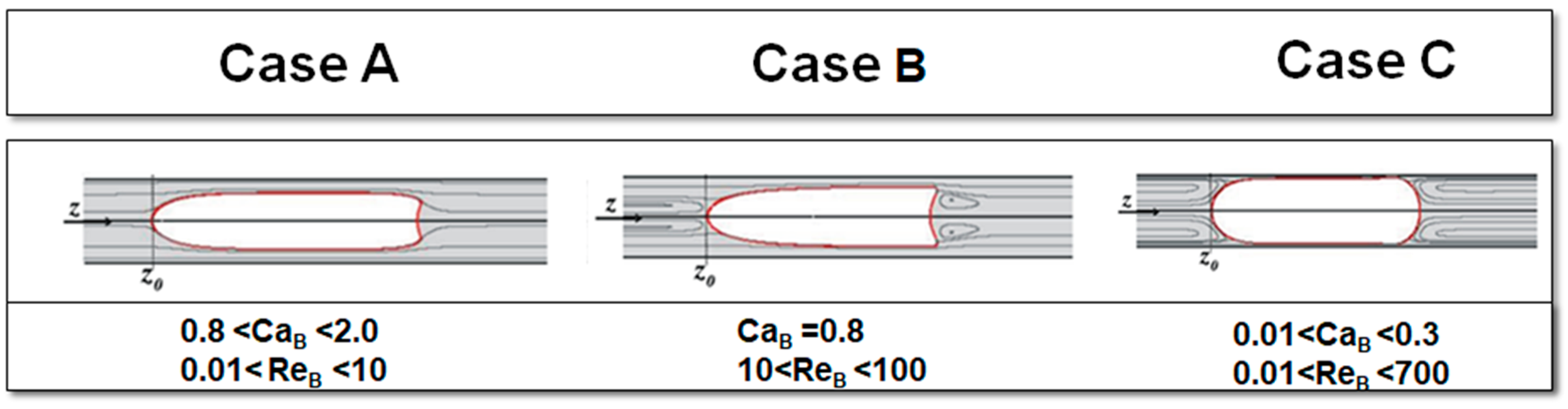
One important example of the referred works is the study performed by Rocha et al. [18]. This study was based on the application of CFD techniques, and numerical results of the bubble shape, velocity as well as film thickness were reported for 0.01 < Ca_B < 2 and 0.01 < Re_B < 700. The authors also suggest the existence of three distinct flow behaviors/categories of gas–liquid slug flow in mili/micro-channels (Figure 1):

• In scenarios associated with high Ca_B, the bubble moves faster than the liquid phase that is absent of recirculation zones (assuming a reference frame moving with the bubble—MRF). It was also predicted the presence of a liquid film between the bubble and the wall—Case A.
• For intermediate values of Ca_B, the bubble still moves faster than most of the liquid however, a closed recirculation wake appears below the bubble tail. The liquid film between the bubble and the wall is also present—Case B.
• Finally, for low values of Ca_B, the bubble and liquid phase flow with similar velocity. This scenario involves the presence of semi-infinite recirculation regions (in MRF) ahead and behind the bubble. Additionally, decreasing the Ca_B leads to recirculation regions that occupy a higher cross-sectional area—Case C.

The CFD software used on the work of Rocha et al. [18] was ANSYS Fluent^® (16.2). This is a commercial package that is quite robust and provides the user with solvers for multiphase flow that are already implemented and ready to use. An important example is the Volume of Fluid (VOF) methodology which is the most appropriate to describe slug flow systems. The VOF code of ANSYS Fluent^® has been widely tested in this kind of system with very good results [15,18,19,20]. However, the choice for this type of package does not include solely advantages. Since it is a commercial option, it requires a paid license. On the other hand, the costs involved contribute to ensuring that the software is reliable, that is properly tested, validated and supported by an expert engineering team. Another disadvantage could be the fact that the source code of methods/solvers is not fully available to the user to adapt to his specific needs, making it more of a black box where the manipulation of the models is not as straightforward.

There are some alternatives already available that address these concerns and make them stronger points. Currently, one of the most important, with a fast-growing community (users and developers), is the Open Source Field Operation and Manipulation (OpenFOAM^®) software package. OpenFOAM^® is an open-source C++ library where the code is fully accessible and modifiable enabling the users to solve and manipulate the data of problems in continuum mechanics [21]. As a downside, it is not as well supported as a commercial solution and it requires more thorough validation for each use case.

When solving gas–liquid systems, one of the major concerns is to set a good method/technique to track the gas–liquid interface. It is particularly difficult to compute with a high level of accuracy the forces and movements associated with this region. This issue becomes even more crucial when dealing with smaller scales where the capillary forces are more relevant.

A comparison of how a gas–liquid slug flow system in micro-channels can be handled with ANSYS Fluent^® and OpenFOAM^® will be the main goal of the present work. In the simulations with ANSYS Fluent^®, the interface tracking was made with the VOF methodology [22] already implemented in the software which is coupled with the Piecewise linear interface calculation (PLIC) scheme for interface reconstruction [23].

OpenFOAM^® also presents different alternatives to solve this kind of multiphase flow issues like the ones associated with interFoam [24] and interFlow solvers [25]. The former option (interFoam) applies the MULES—Multidimensional Universal Limiter with Explicit Solution—which is an incompressible method that already includes the VOF methodology with an interfacial compression flux term. One of the main advantages of this solver is the ability to preserve the volume (which is also present on interFlow [25]). However, for some systems, it may also be inaccurate in its solution of the interface advection problem, especially for surface tension-dominated flows where the computed curvatures present deviations of 10% when compared with the analytical solutions [24].

The interFlow solver is an implementation of the isoAdvector approach. The isoAdvector also uses the VOF as a stepping-stone but presents geometric considerations both for the interface reconstruction step as well as for the interface advection step [25].

As aforementioned, the main objective of this work is to compare numerical results obtained with different methods to solve the gas–liquid interface from OpenFOAM^® and ANSYS Fluent^® for a specific micro-scale gas–liquid scenario and, based on these results, perform a detailed assessment of the feasibility of the open-source alternative to describe the referred systems. For that purpose, simulations of the flow of individual Taylor bubbles through a co-current liquid phase inside a microchannel were performed. The physical properties (density and viscosity) and flow conditions (liquid velocity) of the gas–liquid systems were chosen to create three representative cases (Cases A, B and C) that address the different sub-patterns identified in micro-scale slug flow. The simulation of these cases with the chosen numerical approaches (VOF with PLIC in ANSYS Fluent^®; interFoam and interFlow in OpenFOAM^®) provides a good and solid base for comparison and evaluation of their application to this kind of scenario.

2. Materials and Methods

2.1. Governing Equations

In terms of governing equations of the problem, both the continuity and momentum equations were already pre-implemented in the software:

$$\frac{\partial }{\partial t}\left(\rho \right)+\nabla .\left(\rho \overrightarrow{u}\right)=0$$

(3)

$$\frac{\partial }{\partial t}\left(\rho \overrightarrow{u}\right)+\nabla .\left(\rho \overrightarrow{u}\overrightarrow{u}\right)=-\nabla p+\nabla .\left(\stackrel{=}{\tau }\right)+\overrightarrow{F_{\sigma }}$$

(4)

where $p$ stands for pressure, $\overrightarrow{u}$ for the velocity vector and $\stackrel{=}{\tau }$ for the stress tensor. The term associated with gravitational forces is neglected since the cases in study are in microscale where these forces are negligible.

To solve the gas–liquid interface, the Volume of Fluid (VOF) method was chosen:

$$\frac{\partial }{\partial t}\left({\alpha }_G\right)+\overrightarrow{u}.\nabla {\alpha }_G=0$$

(5)

The continuum surface model was applied to account for the surface tension forces at the interface:

$$\overrightarrow{F_{\sigma }}=\sigma \kappa \frac{\rho \nabla {\alpha }_G}{0.5\left({\rho }_G+{\rho }_L\right)}$$

(6)

where $\kappa =-\nabla .\frac{\nabla {\alpha }_G}{\left|\nabla {\alpha }_G\right|}$.

2.2. ANSYS Fluent^® simulations

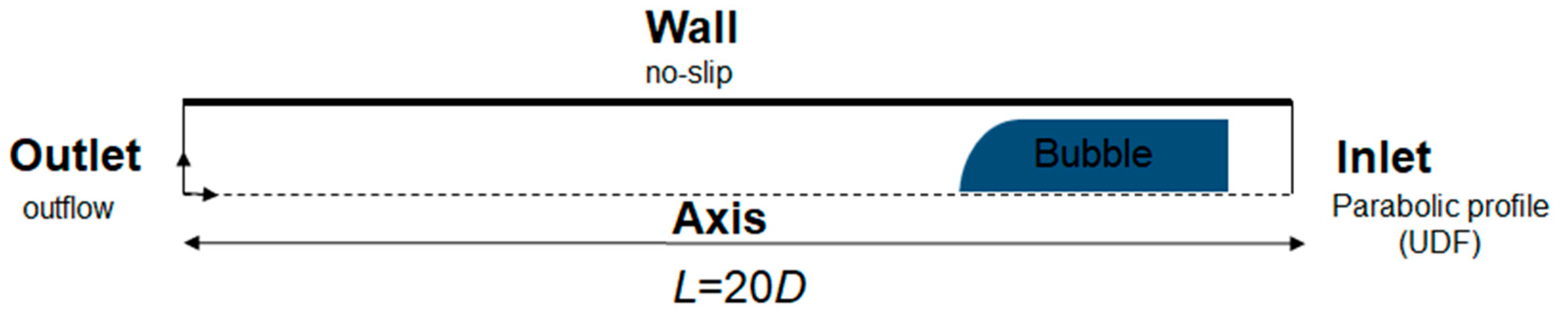
The first set of simulations were performed in ANSYS Fluent^® 16.2. A 2D domain (assuming axisymmetry) was drawn representing half of a cylindrical domain with a length 20 times larger than the diameter (D = 100 μm)—Figure 2. A uniform mesh with 100 × 4000 elements was generated in this domain. Inside the domain, a bubble with an approximated shape (quarter of a circle connected to a rectangle) was added. The bubble base is set at 1.5 D from the Inlet and has a length of 3 D and a maximum width of 0.455 D.

As for the boundaries of the domain: (1) the no-slip condition was applied along the Wall; (2) the parabolic velocity profile typical of laminar flow was imposed at the Inlet; (3) and at the Outlet, a static pressure value was defined as constant. The simulations were performed in a transient state and the conditions applied always kept the flow under the laminar regime.

Regarding the numerical schemes, PISO (“Pressure-Implicit with splitting of operators”) was chosen to solve the discretized velocity-pressure coupled momentum equation, PRESTO! for the pressure interpolations, QUICK to discretize the momentum equation and “Green-Gauss Node Based” to compute the discretized gradients of the scalars.

Since simulations are in a transient state, an explicit time-marching scheme with a maximum Courant number (Co) of 0.25 was used. The time step was variable and the function of Co. Residuals below 1.0 × 10⁻⁶ were set to achieve numerical convergence of the solution.

2.3. OpenFOAM^® simulations

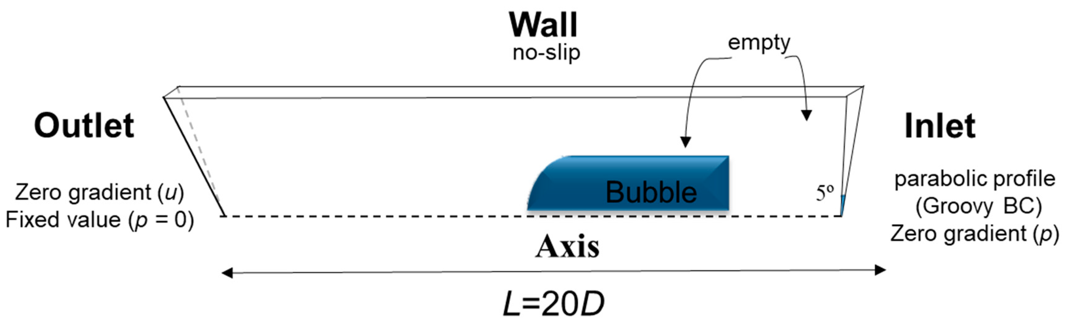
A similar set of simulations was also solved using OpenFOAM^® software. Contrary to the case described in Section 2.2, the domain now used is a slice of a cylinder instead of a 2D rectangle. This is because, by default, OpenFOAM^® was developed to work only with 3D mesh elements. The equivalent domain (see Figure 3) was built as a section of the tube with a wedge angle of 5º and the same dimensions of the domain in Section 2.2 (diameter of 100 μm and a length of 20 diameters). The mesh was built using the blockMesh utility that is part of the OpenFOAM^® and where 100, 1 and 4000 divisions along the x, y and z axes were set, respectively.

Once again, a bubble was added to the domain. This bubble is the combination of a sphere with a radius of 0.455 D connected to a cylinder. The combination of both shapes leads to a bubble with 3 D of length that is placed at 1.5 D from the Inlet (the reference point is the bubble base).

In terms of velocity at the boundaries: laminar parabolic velocity profile was imposed at the Inlet, a no-slip condition was set at the Wall, a symmetryPlane condition at the Axis, and a zeroGradient type was considered at the Outlet. For the pressure variable, a fixed zero value was imposed at the Outlet, while for the Wall and Inlet a condition of zeroGradient was considered. The solution was also initialized with only liquid phase (α = 1) present in the domain with the Inlet being defined with a fixed value of 1. The Outlet and Wall are defined as zeroGradient. The bubble (α = 0) was subsequently added using the setFields utility of OpenFOAM^®. The bubble is defined with an approximated shape (a quarter of a circle for the nose linked to a rectangle for the bubble body) and with a velocity equivalent to the one predicted in previous work [18].

Two different solvers of OpenFOAM^® were tested in this work: interFoam [24] and interFlow [25]. Both options solve the Navier–Stokes equations for two incompressible, isothermal, and immiscible fluids. Each solver is supported, respectively, on MULES and isoAdvector approaches to track and define the gas–liquid interface.

To set the α_G, the following equations are considered:

$$\frac{\partial {\alpha }_G}{\partial t}+\frac{\partial {\alpha }_G{u}_j}{\partial x_j}=0$$

(7)

MULES uses a interface compression by adding a purely heuristic term:

$$\frac{\partial \alpha }{\partial t}+\frac{\partial {\alpha }_G{u}_j}{\partial x_j}+\frac{\partial }{\partial x_j}\left({\alpha }_G\left(1-{\alpha }_G\right)u_j^r\right)=0$$

(8)

with $u_j^r=\min \left(c_{\alpha }\left|F_f\right|\left|s_f\right|, max\left[\left|F_f\right|\left|s_f\right|\right]\right)n_{f,j}$ and where $c_{\alpha }$ is a user-defined value that determines the strength of the compression, $F_f$ the face flux, $s_f$ the face area vector normal to the face pointing out of the cell and $n_{f,j}$ is the component j of the interface normal.

The isoAdvector presents a different approach. It does not solve Equation (7) but identifies the interface using an isoline. After that, the exact position is advected in a geometric manner.

An effort to approximate the methods here used with those in ANSYS Fluent^® was made; for example, PISO scheme was used to couple the velocity-pressure for all methods. The options for the numerical schemes chosen in this study are represented in

Table 1. Schemes chosen when using interFoam and interFlow.

	interFoam	interFlow
ddtSchemes	Euler	Euler
gradSchemes	Gauss linear	Gauss linear
divSchemes
div(rho*phi, u)	----	Gauss limitedLinearV 1;
div(rhoPhi, u)	Gauss linear Upwind grad (U);	Gauss limitedLinearV 1;
div(phi, alpha)	Gauss van Leer;	Gauss vanLeer;
div(phi, alpha1)	----	Gauss HRIC;
div(phirb, alpha)	Gauss linear;	Gauss interfaceCompression;
div((muEff*dev (T(grad(U)))))	----	Gauss linear;
div((rho*nuEff)*dev2(T(grad(U))))	Gauss linear;	Gauss linear;
laplacianSchemes	Gauss Linear corrected	Gauss Linear corrected
interpolationSchemes	linear;	linear;
snGradSchemes	corrected;	corrected;

.

The Courant Number was set to control the use of the variable time-step and was adapted to each case but always lower than 0.25. Residuals below 1.0 × 10⁻⁶ were also set to get the solution convergence.

Table 2. Main parameters that characterize each case in the study where ρ stands for the liquid density and μ for the liquid viscosity.

	Physical Properties	Dimensionless Groups	Simulation Parameters
Case A	ρ = 1000 kg·m−3 μ = 3.74 × 10−2 Pa·s	CaB = 10 ReB = 2.0	Co = 0.25 Δt = 10−7
Case B	ρ = 1000 kg·m−3 μ = 7.48 × 10−3 Pa·s	CaB = 100 ReB = 0.8	Co = 0.25 Δt = 10−8
Case C	ρ = 1000 kg·m−3 μ = 4.58 × 10−2 Pa·s	CaB = 0.1 ReB = 0.03	Co = 0.25; 0.20 *; 0.10 * Δt =10−6; 10−7 *; 10−8 *; 10−9 *

* refers to different tests performed using OpenFOAM to improve the quality of results.

summarizes the main parameters of each case that will be discussed.

3. Results

As previously mentioned, the reference scenario for this numerical study is the Taylor bubble flow in microscale. Three cases with different dimensionless numbers were addressed in both ANSYS Fluent^® and OpenFOAM^® and the corresponding results will be presented and discussed along this section. For each case, the results for the main hydrodynamic characteristics of the flow obtained with each software, will be shown and compared. It is important to notice that the application of the commercial package (ANSYS Fluent^®) to simulate this kind of gas–liquid system was already validated in previous work [18].

3.1. Case A

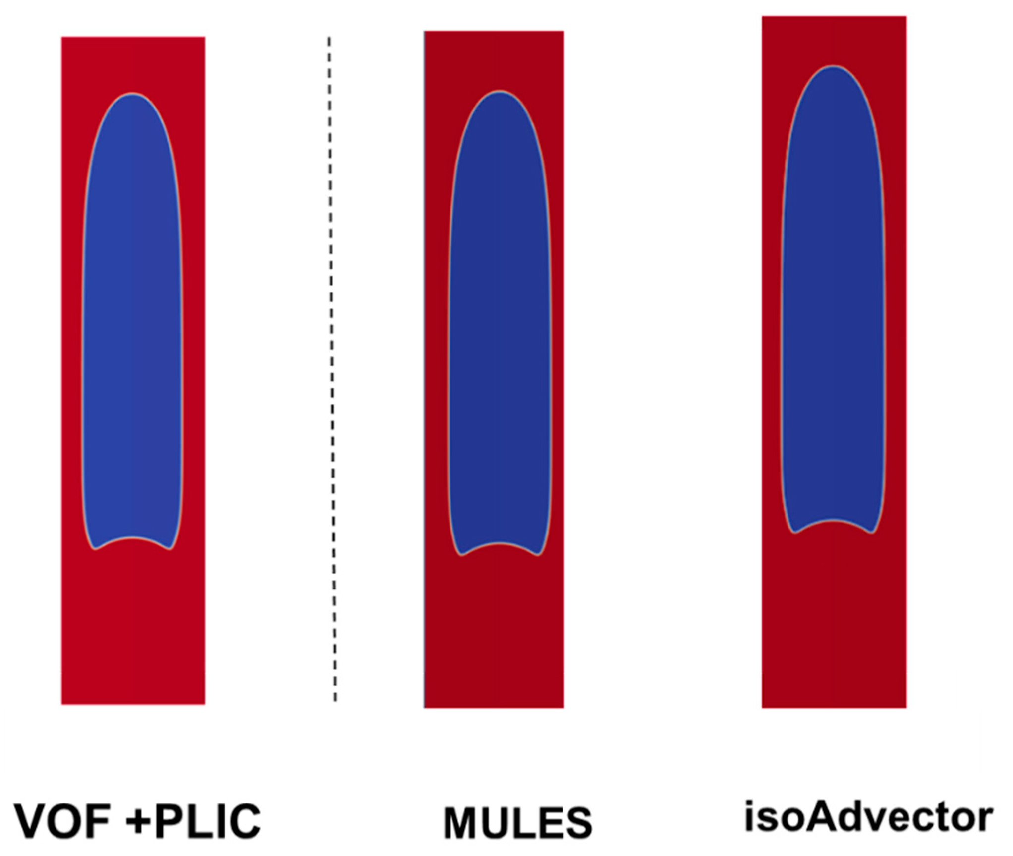
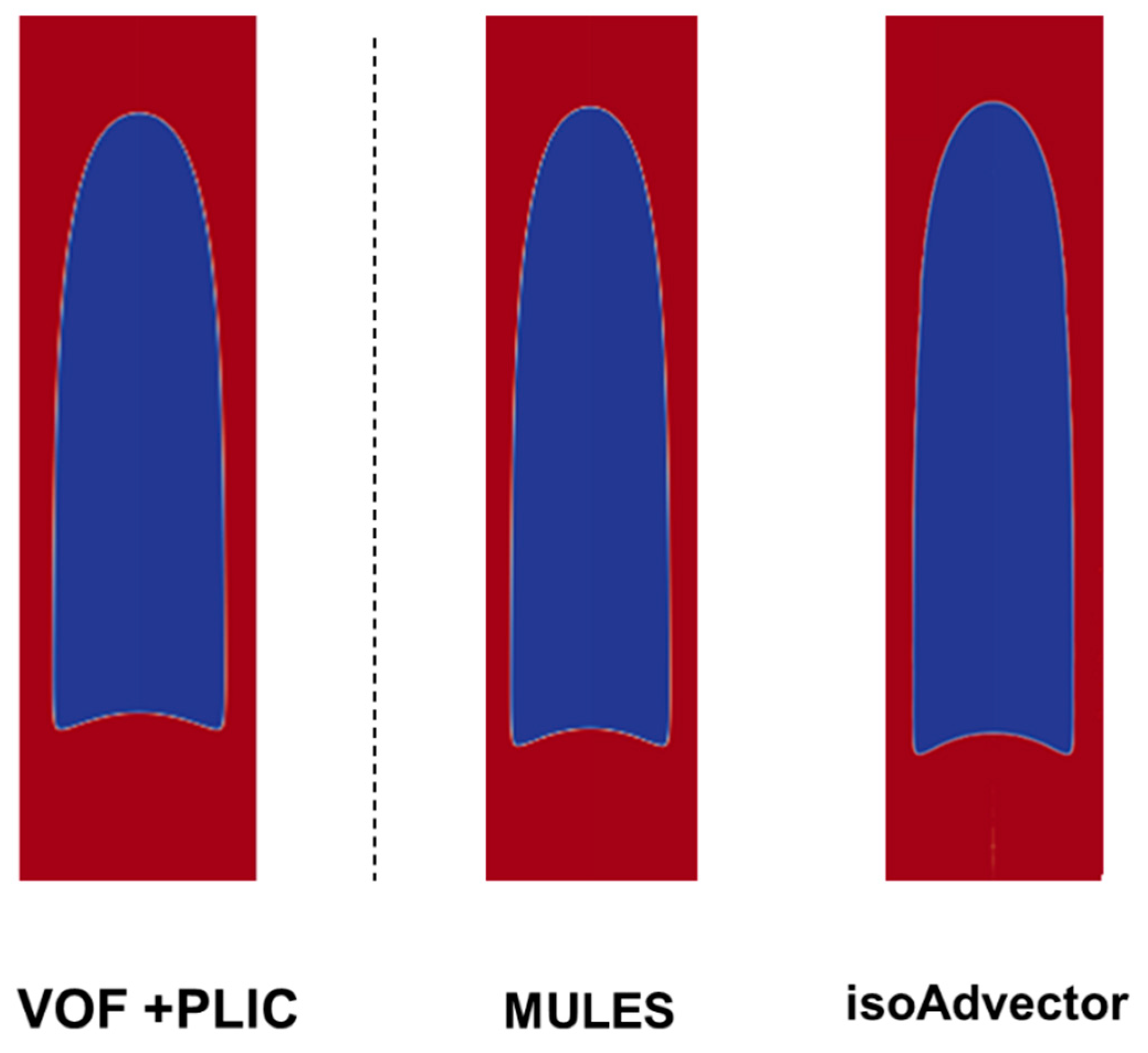
Case A is characterized by the dimensionless numbers of Re_B = 10 and Ca_B = 2.0. The results revealed the presence of a characteristic Taylor bubble with a velocity higher than the surrounding liquid that does not present any recirculation regions. As expected, it was obtained a liquid film separating the bubble from the wall. In Figure 4, the bubble shape acquired with each method is represented. For all the methods used to solve this system, the bubble presented a similar shape: a slender nose and a tail with a concave shape.

One of the most important hydrodynamic features of slug flow is the liquid film thickness. The values obtained for this feature using VOF+PLIC (ANSYS Fluent^®), MULES (OpenFoam^®) and IsoAdvector (OpenFoam^®) are compared with the expression of Han and Shikazono [26]:

$$\frac{\delta }{D}=\frac{0.670{\mathrm{Ca}}_{\mathrm{B}}{}^{2/3}}{1+3.13{\mathrm{Ca}}_{\mathrm{B}}{}^{2/3}+0.504{\mathrm{Ca}}_{\mathrm{B}}{}^{0.672}{\mathrm{Re}}_{\mathrm{B}}{}^{0.589}-0.352{\mathrm{We}}_{\mathrm{B}}{}^{0.629}}$$

(9)

where ${\mathrm{We}}_{\mathrm{B}}={\mathrm{Re}}_{\mathrm{B}}{\mathrm{Ca}}_{\mathrm{B}}$.

The numerical values of the liquid thickness are presented in Table 2 and are all very close to the theoretical predictions. The thickness acquired using isoAdvector is the closest one to the theoretical value (deviation below 1%).

From the simulation data, the bubble velocity for each different solver was also determined and compared (

Table 3. Thickness of the film predicted by Equation (9) and obtained by the different numerical approaches as well as the deviation between the numerical and theoretical values. Bubble velocity for the different numerical approaches as well as the value predicted by Equation (10).

	Theoretical	VOF+PLIC	MULES	IsoAdvector
$\frac{\delta }{D}$	1.57 × 10−1	1.63 × 10−1 ± 3.78%	1.55 × 10−1 ± 1.02%	1.56 × 10−1 ± 0.78%
$u_b$ (m·s−1)	3.5	3.6	3.5	3.5

). The data were compared with the expression also used on Rocha et al. [18] and where the film velocity is assumed as near zero:

$$u_b=\frac{1}{1-{\frac{\delta }{R}}^2} u_L$$

(10)

For both solvers in Open FOAM^® (MULES and isoAdvector), the bubble velocity obtained was 3.5 m·s⁻¹. With ANSYS Fluent^®, a slightly higher velocity of 3.6 m·s⁻¹ was predicted. Despite the slight differences, both methods seem to be able to predict fairly precise bubble velocity values.

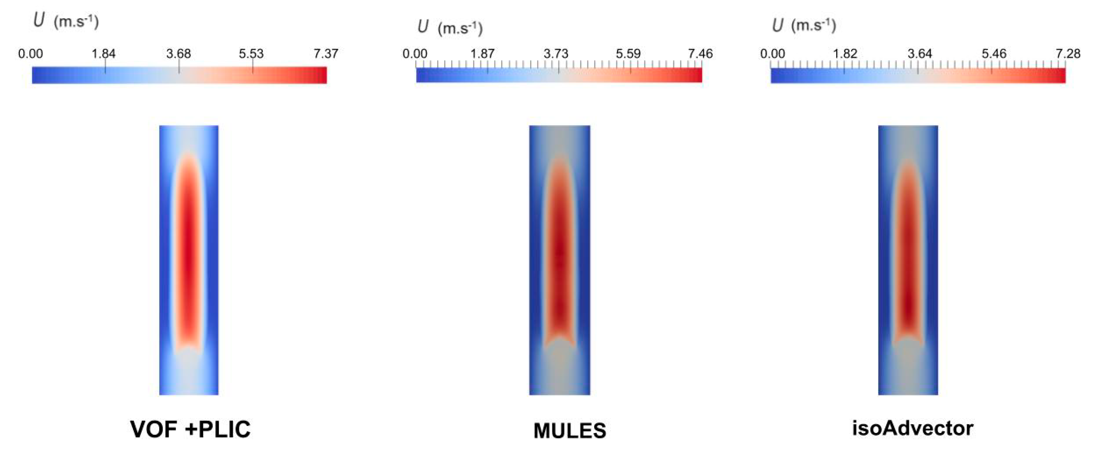
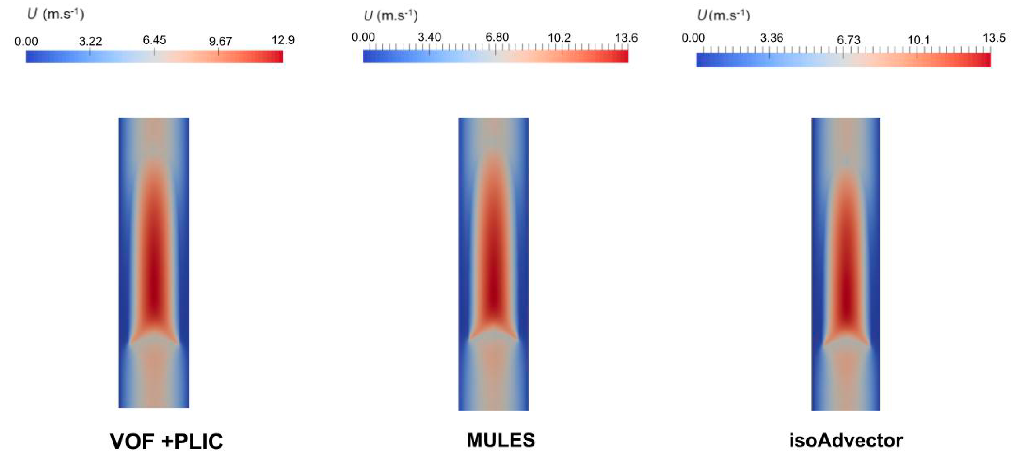
Regarding the velocity fields, the corresponding contours are represented in Figure 5 where U is the magnitude of the velocity vector.

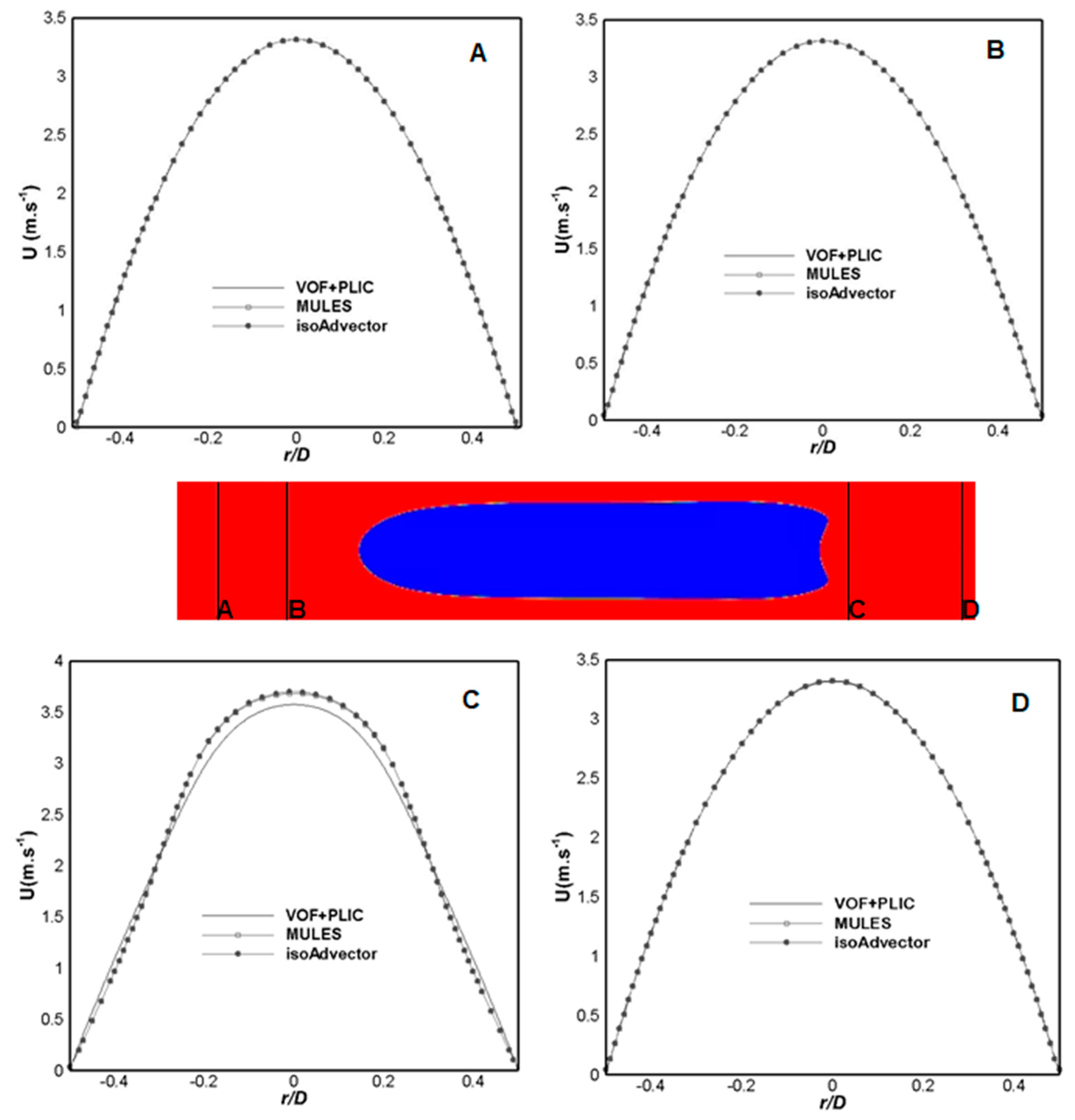
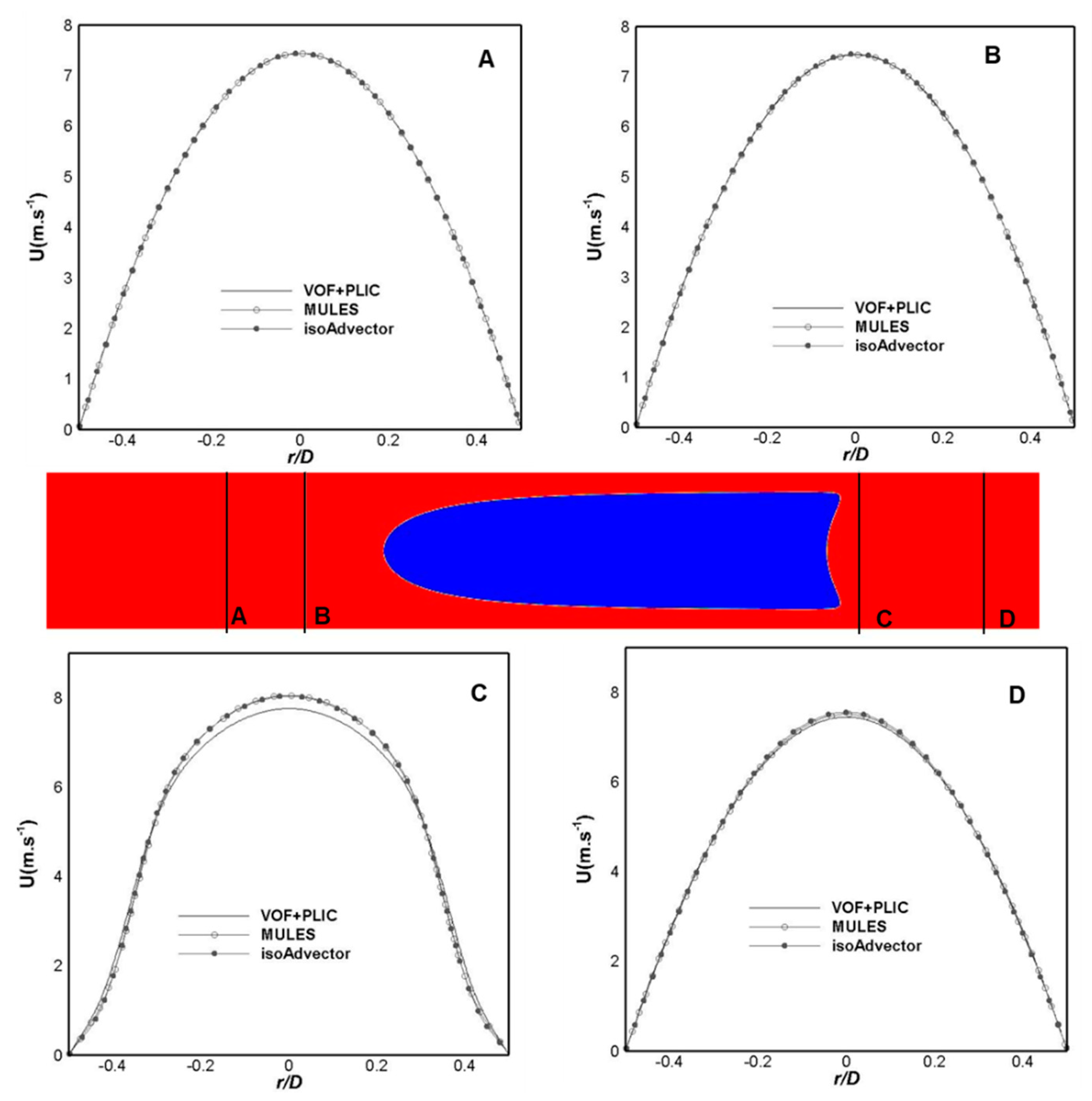
Small differences were detected in the velocity field values acquired using the different methods, however, the velocity fields obtained with ANSYS Fluent^® or OpenFOAM^® appear to be slightly different at the bubble rear. Taking this into consideration, some lines were defined along the domain having the bubble nose tip and the point where the tail intersects the axis as points of reference. For those lines, velocity profiles extracted above and below the bubble are represented in Figure 6.

The profiles show that the velocity behavior above the bubble and at one diameter from the tail are fairly similar no matter the method used, i.e., the profiles overlap. However, as suggested by Figure 5, there is a difference (deviation of 3% at r/D = 0) in the velocity in the position closest to the tail (C), where the values acquired using VOF + PLIC (ANSYS Fluent^®) are lower than the ones predicted using OpenFOAM^®.

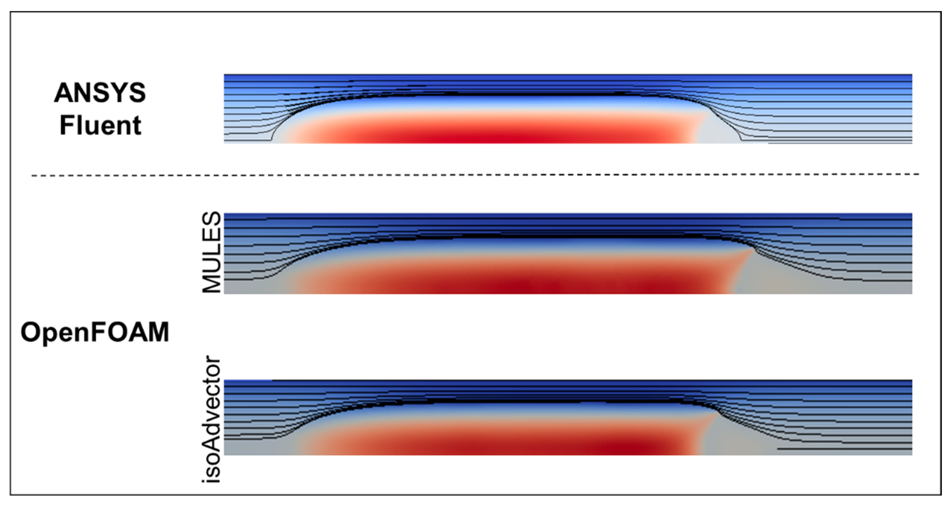
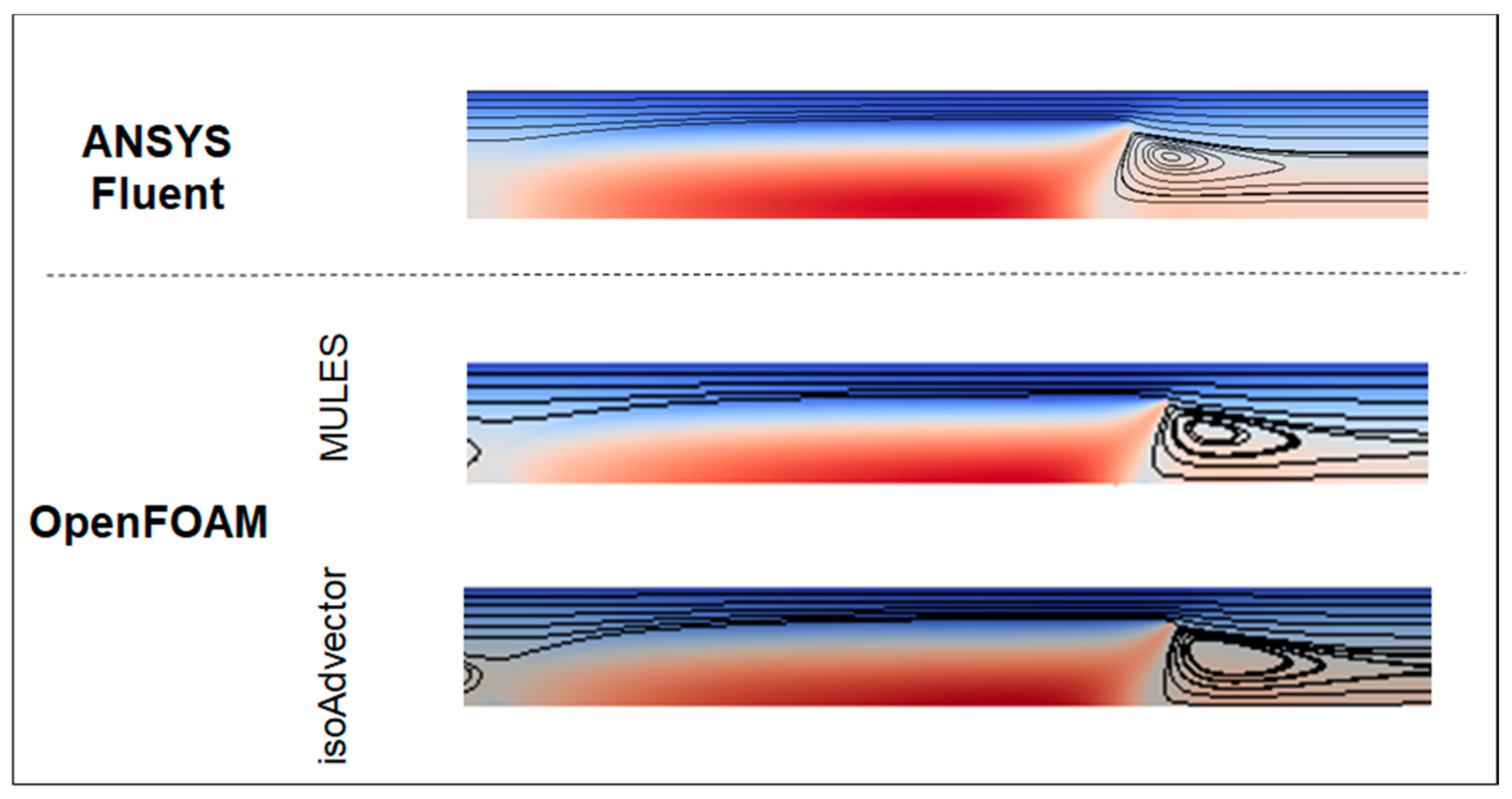
To check the type of liquid recirculation around the bubble, the streamlines obtained with the different approaches are also presented for Case A—Figure 7.

As expected, the streamlines do not show any recirculation areas, i.e., the three solvers seem to point to the same liquid flow patterns around the bubble.

3.2. Case B

Case B is characterized by the dimensionless numbers of Re_B = 100 and Ca_B = 0.8. This case presents the characteristic shape of a Taylor bubble and, when compared with the previous case, the most obvious difference is in the tail shape—Figure 8. Once again, Figure 8 presents the contours of the phases acquired using ANSYS Fluent^® and OpenFOAM^®. It should also be pointed out that, for this case, there will be a closed recirculation area below the tail (assuming MRF).

Following the same strategy as in Case A, the analysis started with the liquid thickness along the film region. This important feature was once again determined and compared with the theoretical prediction of Equation (9)—

Table 4. Thickness of the film acquired through Equation (9) and the different numerical approaches as well as the deviation between the numerical and theoretical values. Bubble velocity obtained with different numerical approaches as well as the value predict by Equation (10).

	Theoretical	VOF+PLIC	MULES	IsoAdvector
$\frac{\delta }{D}$	1.23 × 10−1	1.27 × 10−1 ± 3.47%	1.33 × 10−1 ± 8.36%	1.3 × 10−1 ± 5.91%
$u_b$ (m·s−1)	6.5	6.7	6.8	6.8

.

The values numerically acquired are all in reasonable agreement with the prediction made by Equation (9). Additionally, the result taken with the VOF + PLIC shows the lowest deviation from the theoretical value.

The bubble velocity was also determined, and the results are also presented in Table 4. As previously, the three approaches produced very similar bubble velocities, with the solvers implemented in OpenFOAM^® leading to slightly higher velocities.

The velocity fields obtained with the different solvers are also compared (Figure 9). From this Figure, the contours do not reveal any significant difference.

The velocity profiles for predefined positions above and below the bubble were extracted and are compared in Figure 10.

Similarly to the set of results from the previous case, the velocity profiles for Case B tend to overlap in the same positions (A, B and D) and regardless of the solver used. The main difference is again on position C which corresponds to the region where the wake region is still developing (this region is more visible in Figure 11). Between the velocity profiles, there is a maximum deviation of about 3.4% for the results of VOF + PLIC and IsoAdvector at r/D = 0.

Finally, the streamlines extracted from the simulation data of each solver are represented taking the bubble velocity as a reference—Figure 11. The streamlines present a similar behavior and, more importantly, show the presence of a closed recirculation area behind the bubble (consistent with laminar wake).

3.3. Case C

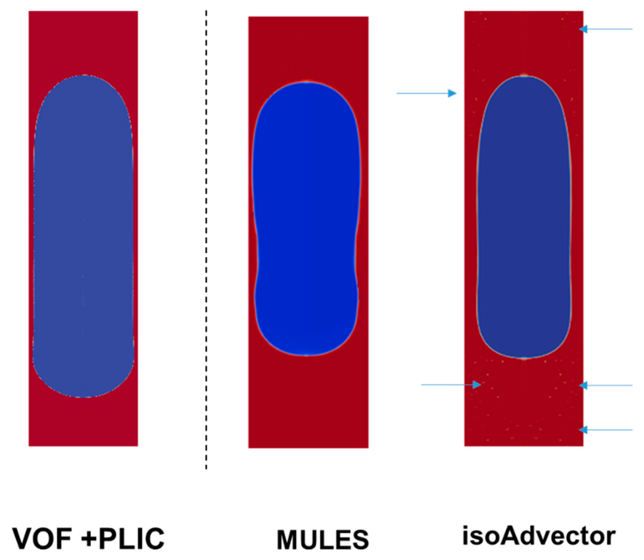
The last case studied in this work is the one with the lowest Capillary number (Ca_B = 0.03) and with a Re_B = 0.1. This case is characterized by the presence of a bubble where both nose and tail present a round shape. Once again, this system was simulated with different solvers. In Figure 12, the simulation results for the bubble shape are represented. As can be seen, and contrary to the previous cases, the bubble shape obtained is not independent of the approach being used.

Figure 12 shows that the bubble acquired using ANSYS Fluent^® is the widest in both length and width. Using MULES, the bubble shape includes a depression in the film region. With isoAdvector, it was observed the presence of small bubbles dispersed along the domain. The bubble shape form is similar to the one acquired with ANSYS Fluent^®, but it is shorter and thinner. Around the bubble, acquired using interFlow, it can be observed the presence of small portions of gas. The presence of these small structures (blue arrows in Figure 12) may help to justify the difference in the volume of the bubbles acquired using the different methods.

In

Table 5. Thickness of the film acquired with Equation (9) and the different solvers used as well as the deviation between the numerical and theoretical values. Bubble velocity obtained with different numerical approaches as well as the value predicted by Equation (10).

	Theoretical	VOF+PLIC	MULES	IsoAdvector
$\frac{\delta }{D}$	4.96 × 10−2	4.7 × 10−2 ± 5.15%	1.15 × 10−1 + 132%	1.11 × 10−1 + 122%
$u_b$ (m·s−1)	0.046	0.046	0.046	0.049

, the liquid film thickness obtained with each approach is compared with the theoretical prediction of Equation (9). As expected by the visualization of Figure 12, there are significant differences depending on the solver applied. In this case, the thickness obtained using the VOF + PLIC is the one that gets closer to the theoretical value (with an error of about 5%), while the thicknesses predicted by MULES and isoAdvector are over two times the theoretical value.

These numerical results of bubble shape and film thickness indicate that the solvers implemented in OpenFOAM^® may not be the most suitable to solve cases with small Capillary numbers.

Finally, the simulation results of the bubble velocity for case C are also presented in Table 5. Opposite to what happened in the previous cases, isoAdvector predicts a slightly higher bubble velocity than the other two methods.

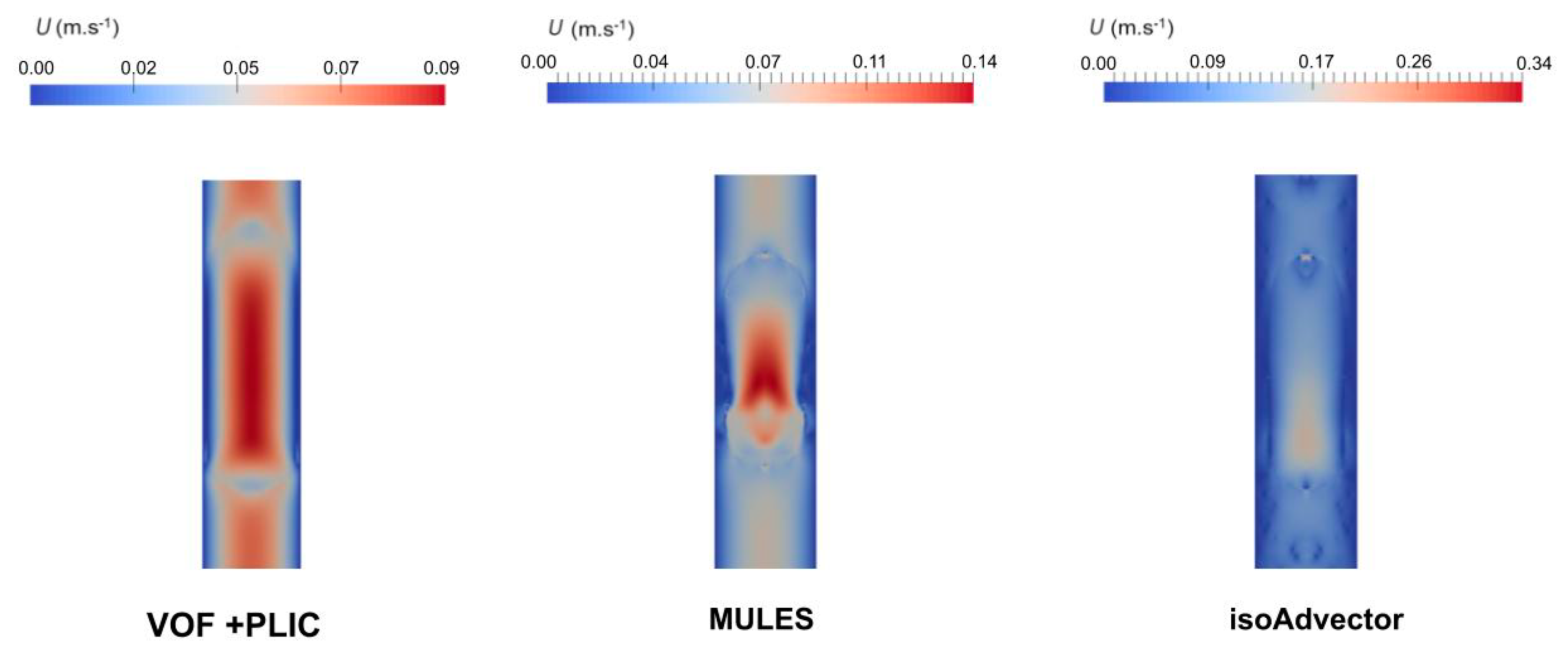
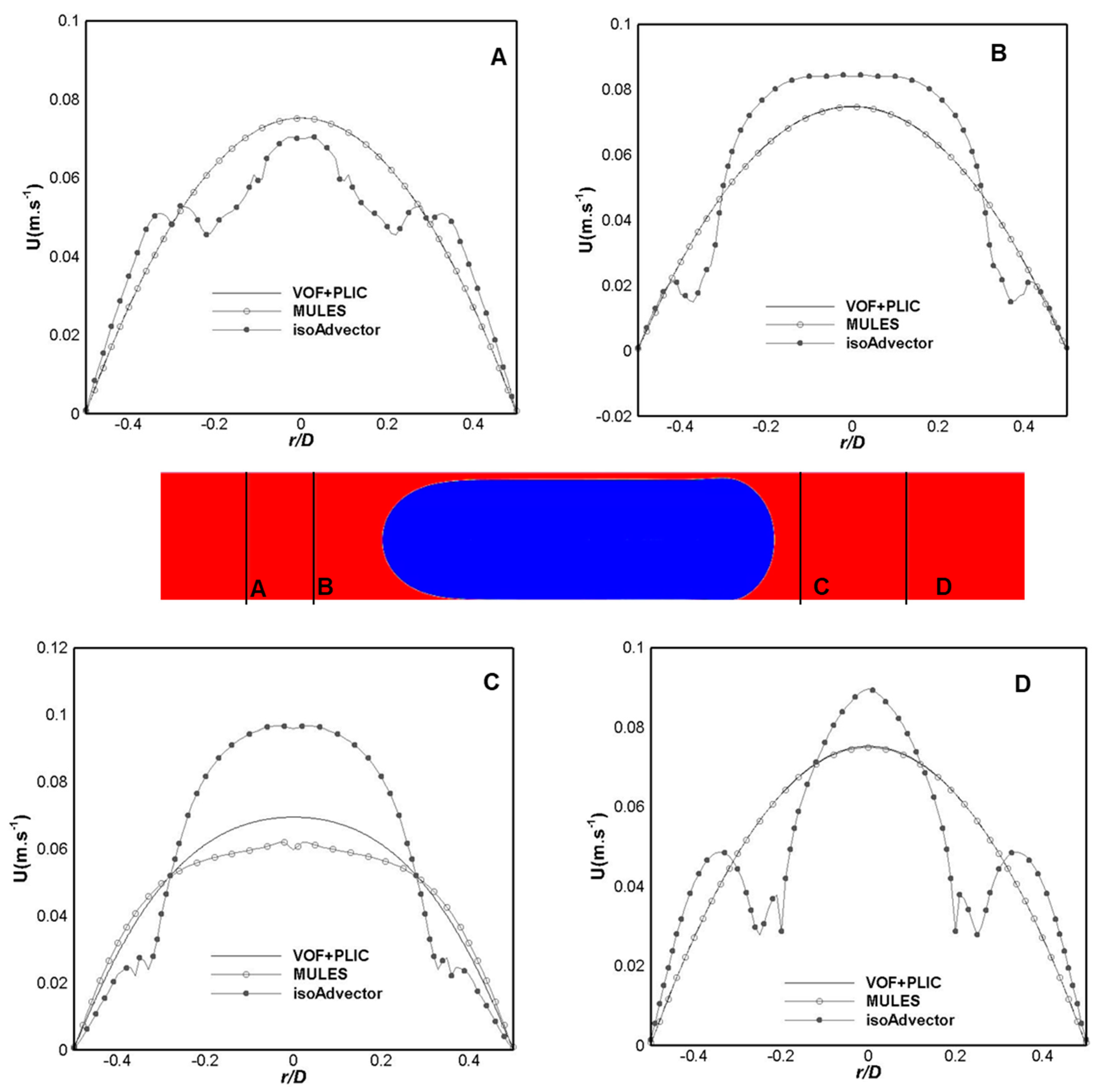
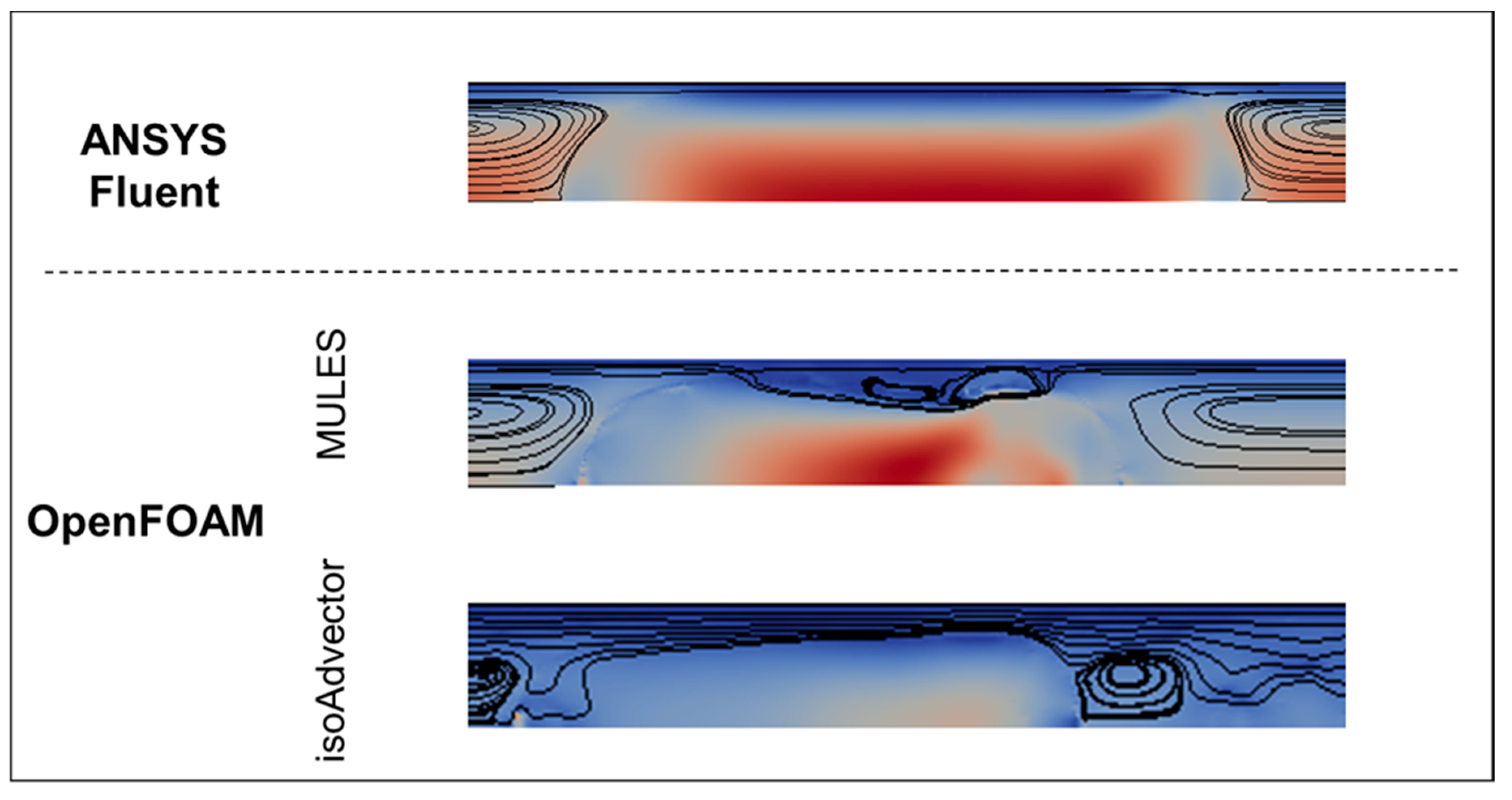
The velocity fields were also represented for the different approaches—Figure 13. From this figure, it is easy to verify that the results of the velocity contours differ significantly depending on the solver in use. This observation is reinforced by the velocity profiles extracted in several positions (Figure 14), as well as by the representation of streamlines around the bubble (Figure 15).

The more obvious explanation for these disturbances along the velocity fields is the arising of spurious currents in the numerical codes of OpenFOAM^®. Spurious or parasitic currents are unphysical numerical flows that usually appear along the bubble interface [27,28], and are mainly due to the method used to solve the effect of the surface tension—Continuum Surface Force [29,30]. These unphysical currents along the interface can affect the prediction of the velocity field or, in more extreme conditions, cause the break-up of the interface being especially problematic for systems characterized by surface tension dominated flows (Ca_B < 0.01) [27,28,30].

According to the literature, some strategies have been adopted to minimize the presence of these currents [19]: mesh refinement along the interface [31]; use of dynamic mesh adaptation [32]; use of different schemes to solve the interface [33] as well as variations on the CSF technique implementation [34,35]. Some of these options to minimize the parasitic currents are available in ANSYS Fluent^® (HRIC scheme to solve the interface [33]; couple VOF–CSF method with a Height Function method [36]) while for OpenFOAM^® there are some options to improve the tension surface effects implementation [37,38,39]. In this work, the objective was to simulate the slug flow systems using the main solvers without implementing additional functionalities and assess their performance. To improve our results, and following Galusinski and Vigneaux [40], the time-step was decreased (1 × 10⁻⁹ s) and set as a fixed value. However, it was not enough to guarantee the total elimination of the spurious currents for the case with the lowest Capillary number.

4. Conclusions

The present work reports a numerical study on slug flow in micro-channels where three representative cases of different flow sub-patterns were set: (1) Case A, characterized by a high Ca_B number (0.8–2.0) and a high bubble velocity without any recirculation region present; (2) Case B, with an intermedium Ca_B number (0.8), where the bubble still moves faster than the liquid but with a closed recirculation region attached to the bubble bottom; (3) Case C, characterized by a low Ca_B (0.010–0.3)_, where the bubble and liquid flow with approximately the same velocity and, in the liquid, there are recirculation regions above and below the bubble.

The aforementioned cases were solved using different numerical approaches for the gas–liquid interface (VOF with PLIC in ANSYS Fluent^®; interFoam and interFlow in OpenFOAM^®).

The bubble shape, film thickness, bubble velocity as well as the velocity fields were the hydrodynamic features used for comparison of numerical approaches. From the simulation results, it is possible to conclude that for Cases A and B, both approaches correctly predict the flow in the study. Both show a solution where the bubble shapes are similar, and the bubble velocity and thickness of the liquid film are close to the values theoretically expected. The only difference between the values acquired is in the liquid velocity. Just below the bubble, the velocity profiles present small deviations (<3.4%) between them.

As the Capillary number decreases, the ability of the methods implemented in OpenFOAM^® to solve the addressed system also decreases. The results show that both options (interFlow and interFoam) lead to bubbles with unexpected shapes and film thickness is way higher than the theoretical predictions. The rise of spurious currents is a common numerical problem for this type of flow, and it is the main reason for the differences detected. To improve the results, an attempt was made to directly reduce the time-step for the systems in the study (time steps in the order 10⁻⁹ s were considered), but it was not enough to resolve the discrepancies and it led to time-consuming simulations. There are several documented approaches to help the minimization of the occurrence of spurious currents, but they fall outside the scope of this work and will be addressed in the future.

References

- Ganapathy, H.; Al-hajri, E.; Ohadi, M. Mass transfer characteristics of gas—Liquid absorption during Taylor flow in mini/microchannel reactors. Chem. Eng. Sci. 2013, 101, 69–80. [Google Scholar] [CrossRef]
- Ganapathy, H.; Shooshtari, A.; Dessiatoun, S.; Ohadi, M.; Alshehhi, M. Hydrodynamics and mass transfer performance of a microreactor for enhanced gas separation processes. Chem. Eng. J. 2015, 266, 258–270. [Google Scholar] [CrossRef]
- Silva, M.; Miranda, J.M.; Campos, J.; Araújo, J. Mass transfer from a Taylor bubble to the surrounding flowing liquid at the micro-scale: A numerical approach. Microfluid. Nanofluid. 2019, 23, 58. [Google Scholar] [CrossRef]
- Silva, M.; Campos, J.; Araújo, J. Mass transfer from a soluble wall into gas-liquid slug flow in a capillary tube. Int. J. Heat Mass Transf. 2019, 132, 745–761. [Google Scholar] [CrossRef]
- Butler, C.; Cid, E.; Billet-Duquenne, A. Modelling of mass transfer in Taylor flow: Investigation with the PLIF-I technique. Chem. Eng. Res. Des. 2016, 115, 292–302. [Google Scholar] [CrossRef] [Green Version]
- Abiev, R.; Butler, C.; Cid, E.; Lalanne, B.; Billet, A.-M. Mass transfer characteristics and concentration field evolution for gas-liquid Taylor flow in milli channels. Chem. Eng. Sci. 2019, 207, 1331–1340. [Google Scholar] [CrossRef] [Green Version]
- Jia, H.; Zhang, P. Investigation of the Taylor bubble under the effect of dissolution in microchannel. Chem. Eng. J. 2016, 285, 252–263. [Google Scholar] [CrossRef]
- Haase, S.; Murzin, D.Y.; Salmi, T.; Stefan, H.; Yu, M.D.; Tapio, S. Review on hydrodynamics and mass transfer in minichannel wall reactors with gas–liquid Taylor flow. Chem. Eng. Res. Des. 2016, 113, 304–329. [Google Scholar] [CrossRef]
- Asadolahi, A.N.; Gupta, R.; Fletcher, D.F.; Haynes, B.S. CFD approaches for the simulation of hydrodynamics and heat transfer in Taylor flow. Chem. Eng. Sci. 2011, 66, 5575–5584. [Google Scholar] [CrossRef]
- Tsoligkas, A.; Simmons, M.; Wood, J. Influence of orientation upon the hydrodynamics of gas–liquid flow for square channels in monolith supports. Chem. Eng. Sci. 2007, 62, 4365–4378. [Google Scholar] [CrossRef]
- Kreutzer, M.T.; Kapteijn, F.; Moulijn, J.A.; Kleijn, C.R.; Heiszwolf, J.J. Inertial and interfacial effects on pressure drop of Taylor flow in capillaries. AIChE J. 2005, 51, 2428–2440. [Google Scholar] [CrossRef]
- Howard, J.A.; Walsh, P.A. Review and extensions to film thickness and relative bubble drift velocity prediction methods in laminar Taylor or slug flows. Int. J. Multiph. Flow 2013, 55, 32–42. [Google Scholar] [CrossRef]
- Bento, D.; Sousa, L.; Yaginuma, T.; Garcia, V.; Lima, R.A.; Miranda, J.M. Microbubble moving in blood flow in microchannels: Effect on the cell-free layer and cell local concentration. Biomed. Microdevices 2017, 19, 1–10. [Google Scholar] [CrossRef] [Green Version]
- Zaloha, P.; Křišťál, J.; Jiricny, V.; Völkel, N.; Xuereb, C.; Aubin, J. Characteristics of liquid slugs in gas–liquid Taylor flow in microchannels. Chem. Eng. Sci. 2012, 68, 640–649. [Google Scholar] [CrossRef] [Green Version]
- Gupta, R.; Fletcher, D.F.; Haynes, B.S. On the CFD modelling of Taylor flow in microchannels. Chem. Eng. Sci. 2009, 64, 2941–2950. [Google Scholar] [CrossRef]
- Abiev, R.S.; Lavretsov, I. Hydrodynamics of gas–liquid Taylor flow and liquid–solid mass transfer in mini channels: Theory and experiment. Chem. Eng. J. 2011, 176, 57–64. [Google Scholar] [CrossRef]
- Abiev, R.S. Simulation of the slug flow of a gas-liquid system in capillaries. Theor. Found. Chem. Eng. 2008, 42, 105–117. [Google Scholar] [CrossRef]
- Rocha, L.A.M.; Miranda, J.M.; Campos, J.B.L.M. Wide Range Simulation Study of Taylor Bubbles in Circular Milli and Microchannels. Micromachines 2017, 8, 154. [Google Scholar] [CrossRef] [Green Version]
- Wörner, M. Numerical modeling of multiphase flows in microfluidics and micro process engineering: A review of methods and applications. Microfluid. Nanofluid. 2012, 12, 841–886. [Google Scholar] [CrossRef]
- Gupta, R.; Fletcher, D.; Haynes, B.S. Taylor Flow in Microchannels: A Review of Experimental and Computational Work. J. Comput. Multiph. Flows 2010, 2, 1–31. [Google Scholar] [CrossRef]
- Yang, G.; Du, B.; Fan, L. Bubble formation and dynamics in gas–liquid–solid fluidization—A review. Chem. Eng. Sci. 2007, 62, 2–27. [Google Scholar] [CrossRef]
- Hirt, C.; Nichols, B. Volume of fluid (VOF) method for the dynamics of free boundaries. J. Comput. Phys. 1981, 39, 201–225. [Google Scholar] [CrossRef]
- Youngs, D.L. Time-dependent multi-material flow with large fluid distortion. In Numerical Methods for Fluid Dynamics; Morton, K.W., Baines, M.J., Eds.; Academic Press: Cambridge, MA, USA, 1982; pp. 273–285. [Google Scholar]
- Deshpande, S.S.; Anumolu, L.; Trujillo, M.F. Evaluating the performance of the two-phase flow solver interFoam. Comput. Sci. Discov. 2012, 5, 014016. [Google Scholar] [CrossRef]
- Roenby, J.; Bredmose, H.; Jasak, H. A computational method for sharp interface advection. R. Soc. Open Sci. 2016, 3, 160405. [Google Scholar] [CrossRef] [Green Version]
- Han, Y.; Shikazono, N. Measurement of the liquid film thickness in micro tube slug flow. Int. J. Heat Fluid Flow 2009, 30, 842–853. [Google Scholar] [CrossRef]
- Lafaurie, B.; Nardone, C.; Scardovelli, R.; Zaleski, S.; Zanetti, G. Modelling Merging and Fragmentation in Multiphase Flows with SURFER. J. Comput. Phys. 1994, 113, 134–147. [Google Scholar] [CrossRef]
- Zahedi, S.; Kronbichler, M.; Kreiss, G. Spurious currents in finite element based level set methods for two-phase flow. Int. J. Numer. Methods Fluids 2011, 69, 1433–1456. [Google Scholar] [CrossRef]
- Pan, Z.; Weibel, J.A.; Garimella, S.V. Spurious Current Suppression in VOF-CSF Simulation of Slug Flow through Small Channels. Numer. Heat Transf. Part A Appl. 2014, 67, 1–12. [Google Scholar] [CrossRef]
- Harvie, D.J.E.; Davidson, M.; Rudman, M. An analysis of parasitic current generation in Volume of Fluid simulations. Appl. Math. Model. 2006, 30, 1056–1066. [Google Scholar] [CrossRef]
- Gupta, R.; Fletcher, D.; Haynes, B.S. CFD modelling of flow and heat transfer in the Taylor flow regime. Chem. Eng. Sci. 2010, 65, 2094–2107. [Google Scholar] [CrossRef]
- Mehdizadeh, A.; Sherif, S.; Lear, W. Numerical simulation of thermofluid characteristics of two-phase slug flow in microchannels. Int. J. Heat Mass Transf. 2011, 54, 3457–3465. [Google Scholar] [CrossRef]
- Horgue, P.; Augier, F.; Quintard, M.; Prat, M. A suitable parametrization to simulate slug flows with the Volume-Of-Fluid method. Comptes Rendus Mécanique 2012, 340, 411–419. [Google Scholar] [CrossRef] [Green Version]
- Renardy, Y.; Renardy, M. PROST: A Parabolic Reconstruction of Surface Tension for the Volume-of-Fluid Method. J. Comput. Phys. 2002, 183, 400–421. [Google Scholar] [CrossRef] [Green Version]
- Jamet, D.; Torres, D.; Brackbill, J. On the Theory and Computation of Surface Tension: The Elimination of Parasitic Currents through Energy Conservation in the Second-Gradient Method. J. Comput. Phys. 2002, 182, 262–276. [Google Scholar] [CrossRef] [Green Version]
- Guo, Z.; Fletcher, D.F.; Haynes, B.S. Implementation of a height function method to alleviate spurious currents in CFD modelling of annular flow in microchannels. Appl. Math. Model. 2015, 39, 4665–4686. [Google Scholar] [CrossRef]
- Hysing, S. A new implicit surface tension implementation for interfacial flows. Int. J. Numer. Methods Fluids 2005, 51, 659–672. [Google Scholar] [CrossRef]
- Popinet, S.; Zaleski, S. A front-tracking algorithm for accurate representation of surface tension. Int. J. Numer. Methods Fluids 1999, 30, 775–793. [Google Scholar] [CrossRef]
- Meier, M.; Yadigaroglu, G.; Smith, B.L. A novel technique for including surface tension in PLIC-VOF methods. Eur. J. Mech. B/Fluids 2002, 21, 61–73. [Google Scholar] [CrossRef]
- Galusinski, C.; Vigneaux, P. On stability condition for bifluid flows with surface tension: Application to microfluidics. J. Comput. Phys. 2008, 227, 6140–6164. [Google Scholar] [CrossRef] [Green Version]
Figure 1.
Representation of the different sub-patterns in micro-scale slug flow described by Rocha et al. [18].
Figure 2.
Representation of the domain and boundary conditions used with ANSYS Fluent.
Figure 3.
Representation of the domain and boundary conditions used with OpenFOAM®.
Figure 4.
Bubble shape for a case with a ReB = 10 and CaB = 2.0.
Figure 5.
Velocity contours acquired from the different numerical approaches.
Figure 6.
Velocity profiles for different positions produced with different numerical approaches. Position A is at 1D above the nose tip, while B is at 0.5D from the same position. Position C is set at 0.2D from the point where the tail intersects the axis and position D is at 1D after the same point.
Figure 7.
Velocity fields and streamlines around a bubble for a system characterized by CaB = 2.0 and ReB = 10. Numerical results acquired with the different numerical approaches are shown.
Figure 8.
Bubble shape for a case with a ReB = 100 and CaB = 0.8.
Figure 9.
Velocity contours obtained with different numerical approaches.
Figure 10.
Velocity profiles for different positions (above and below the bubble) acquired with different numerical approaches. Position A is at 1D above the nose tip, while B is at 0.5D from the same position. Position C is set at 0.2D from the point where the tail intersects the axis and position D is at 1D after the same point.
Figure 11.
Velocity fields and streamlines around a bubble for a system characterized by CaB = 0.8 and ReB = 100. Numerical results are shown for the different solvers used.
Figure 12.
Bubble shape for a case with a ReB = 0.1 and CaB = 0.03. The blue arrows point to small dispersed bubbles along the domain.
Figure 13.
Velocity contours acquired with different numerical approaches.
Figure 14.
Velocity profiles for different positions above and below the bubble, acquired through the different numerical approaches. Position A is at 1D above the nose tip, while B is at 0.5D from the same position. Position C is set at 0.2D from the point where the tail intersects the axis and position D is at 1D after the same point.
Figure 15.
Velocity fields and streamlines around a bubble characterized by CaB = 0.03 and ReB = 0.1, acquired with the different numerical approaches.