Stability of Optimal Closed-Loop Cleaning Scheduling and Control with Application to Heat Exchanger Networks under Fouling


Department of Chemical Engineering, Imperial College London, South Kensington Campus, London SW7 2AZ, UK
*
Author to whom correspondence should be addressed.
Processes 2020, 8(12), 1623; https://0-doi-org.brum.beds.ac.uk/10.3390/pr8121623
Submission received: 27 October 2020
/
Revised: 28 November 2020
/
Accepted: 3 December 2020
/
Published: 9 December 2020
(This article belongs to the Special Issue Expanding the Horizons of Manufacturing: Towards Wide Integration, Smart Systems and Tools)
Abstract
:Heat exchanger networks subject to fouling are an important example of dynamic systems where performance deteriorates over time. To mitigate fouling and recover performance, cleanings of the exchangers are scheduled and control actions applied. Because of inaccuracy in the models, as well as uncertainty and variability in the operations, both schedule and controls often have to be revised to improve operations or just to ensure feasibility. A closed-loop nonlinear model predictive control (NMPC) approach had been previously developed to simultaneously optimize the cleaning schedule and the flow distribution for refinery preheat trains under fouling, considering their variability. However, the closed-loop scheduling stability of the scheme has not been analyzed. For practical closed-loop (online) scheduling applications, a balance is usually desired between reactivity (ensuring a rapid response to changes in conditions) and stability (avoiding too many large or frequent schedule changes). In this paper, metrics to quantify closed-loop scheduling stability (e.g., changes in task allocation or starting time) are developed and then included in the online optimization procedure. Three alternative formulations to directly include stability considerations in the closed-loop optimization are proposed and applied to two case studies, an illustrative one and an industrial one based on a refinery preheat train. Results demonstrate the applicability of the stability metrics developed and the ability of the closed-loop optimization to exploit trade-offs between stability and performance. For the heat exchanger networks under fouling considered, it is shown that the approach proposed can improve closed-loop schedule stability without significantly compromising the operating cost. The approach presented offers the blueprint for a more general application to closed-loop, model-based optimization of scheduling and control in other processes.
1. Introduction
In batch plants, continuous plants, and general manufacturing plants with multiple processing units, multiple products or time-decaying performance, scheduling of production and maintenance is essential to ensure a feasible and economically profitable operation. The aim of scheduling is to define the production sequence, order, allocation, and timing for execution of all production and maintenance tasks. For example, a closed-loop nonlinear model predictive control (NMPC) approach has been developed to simultaneously optimize the cleaning schedule and the flow distribution for refinery preheat trains under fouling [1]. Production scheduling and maintenance scheduling belong to the same kind of problem (i.e., they follow the same principles, assumptions, and modeling approaches) and, in some instances, have been integrated [2,3,4]. One of the main assumptions used to address these problems is a perfect knowledge of the current and future operating conditions, which includes demand, unit performance, availability, and cost of resources.
However, all processes are by nature dynamic and subject to uncertainty and disturbances. For example, in batch processing, unplanned events such as unit breakdown, new orders, changes in order quantity, performance decay of the unit, and variation in costs and prices affect the performance (technical and economic) and even feasibility of a schedule previously determined [5]. Therefore, a re-evaluation of the scheduling decision is necessary and advantageous. Traditionally, two alternatives schemes have been defined: (i) rescheduling, where the main objective is to recover feasibility of the operation after a (significantly large) disturbance is observed, and (ii) online scheduling, where the schedule is updated at regular intervals [6,7]. Rescheduling can be done via a full re-evaluation of the scheduling problem, via partial modification of the previous scheduling decisions, or by postponing the execution of some actions [8]. Typically, this is done over the same time horizon as the original schedule and with no new decision variables. Most of the approaches for rescheduling are based on heuristics and aim to do minimal, yet significant, modifications to recover feasibility [5]. Some others are based on mathematical programming and solve a nonlinear programming (NLP), mixed integer linear programming (MILP) or mixed integer nonlinear programming (MINLP) problem representing a partial scheduling problem (i.e., with a subset of the decisions fixed based on the solution of the initial schedule) [5,9]. In the above classification, online scheduling uses all available decision variables, and aims to maximize the performance of the system at every evaluation so that it does not just reject disturbances, but also generates improvements when the system dynamics allow so [10]. This alternative relies on the solution of optimization problems in a feedback loop using a receding horizon approach (i.e., the time horizon of each schedule evaluation rolls forward and includes new future decisions). The update interval may be fixed and constant, or conditional to the detection of disturbances to the system.
Online scheduling, also referred to as closed-loop scheduling, aims to automate a production and/or maintenance schedule of a plant despite disturbances and variability. However, it has been noted that such a rolling update of the schedule can produce instability in the operation [10,11]. Schedule instability, also called schedule nervousness, may be loosely defined as changes in scheduling decisions between consecutive updates which are undesired (the opposite defines schedule stability). Such changes often have important consequences for the operation. For example, some tasks may not be included in the scheduling model (or not included in sufficient detail) and a change in schedule requires revising them as well. Some tasks may require manual intervention and some resources may require a long procurement time. If scheduling decisions change too frequently or too suddenly, there may not be sufficient time to implement those tasks or procure those resources. In addition, from the operator perspective, too many and sudden schedule changes may be perceived as “erroneous” and “nonintuitive”, leading the operator to manually overwrite some decisions. This in turn will most likely generate delays in execution, introduce further disturbances to the operation that have to be corrected later on, and negatively affect performance [5,8].
In principle, increasing schedule stability within the closed loop would often facilitate the implementation of scheduling decisions, avoid other disturbances occurring in the long term, and improve the closed-loop performance. This will, however, reduce the ability of the system to react to disturbances. Ensuring a rapid schedule response to changes in conditions and schedule stability are, therefore, both desired objectives.
Refining operations are an example of highly dynamic processes with a high energy demand and environmental impact, which are also subject to many uncertainties and variability. They can benefit from an online optimization of their operation to reduce energy consumption, operating cost, and carbon emissions. A key section of a refinery is the preheat train, a large heat exchanger network that recovers around 70% of the energy in the products of the main distillation column [12]. An efficient operation of this section ensures satisfying the production targets, while reducing energy consumption. However, it is subject to a wide range of disturbances such as changes in flow rates, operating temperature, and crude blends processed (which occur on the timescale of hours or days), as well as to efficiency losses, among which the most important is fouling. To maintain an efficient operation of the preheat train in the presence of such disturbances and process variability, the flow distribution through the network and the cleaning schedule of the units have to be optimized.
Usually, the cleaning scheduling and the flow distribution problems of preheat trains have been considered independently, ignoring the inherent variability of the process, and solved using heuristics [13,14,15]. This leads to suboptimal operations because key elements of the problem are ignored, or to infeasible operations because operating limits (e.g., the firing limit of the furnace, the limit capacity of the pumps) are reached, causing a need for emergency cleaning actions or a reduction in production rates. It has been shown that, for these type of processes, integrating flow control in the network and scheduling of exchanger cleaning is advantageous because of the strong synergies between them [16,17]. Optimizing these two elements in a closed loop is, therefore, important to reject disturbances and improve performance. A closed-loop nonlinear model predictive control (NMPC) approach that does this has been developed [1]. However, to achieve a successful implementation of an online cleaning scheduling and flow control of preheat trains, issues related to schedule stability have to be addressed first. Schedule stability is of particular importance in this application because (i) the time scale involved spans from weeks to years, which requires the integration of short-term and long-term decisions, and (ii) the nature of the scheduling decisions (i.e., cleaning of units) requires planning ahead of the specialized resources necessary (e.g., crews, cleaning equipment, cranes, usually contracted out with long notices). Refinery operators, therefore, invariably demand some stability in the future scheduling decisions. Schedule stability, disturbance rejection, and performance optimality are all desired objectives for the problem at hand.
Several approaches have been proposed to balance this trade-off between schedule stability and closed-loop schedule performance in various applications related to batch or manufacturing processes. However, to our knowledge, they have not been proposed related to maintenance or cleaning scheduling. Dynamic effects and variability have been considered by using heuristic algorithms to modify the starting time of the task online [18], by solving an MILP problem that swaps the order or allocation of the task to minimize wait time [19], and by using constraint programming to repair the schedule [20]. All of these methods relay an incumbent schedule as a reference and ignore the effects on economic performance. Other rescheduling approaches penalize in an objective function the changes with respect to the incumbent schedule and may include penalties for reallocation of tasks [21], penalties for changes in the starting time of tasks [22], or a more detailed discrimination of all rescheduling costs (i.e., starting time deviation cost, unit reallocation cost, resequencing cost) as penalties in the objective function [8]. As noted, most of these approaches are designed to be used reactively to recover feasibility when large disturbances are observed and not online for closed-loop optimization of a schedule. An early system for online scheduling (SuperBatch) dealt with highly complex processing configurations (plant, recipes, orders, etc.) in batch manufacturing. Schedules were updated every minute, adjusting for external and process variations on a rapid basis, using an unpublished heuristic method evolved from [18]. The system was successfully applied industrially to scheduling and design of very complex, large-scale food productions [23,24] (Figure 1).
In online or closed-loop scheduling, variability is considered explicitly on a rolling horizon. In this case, the objective function or the constraints of the scheduling problem can be modified to additionally include closed-loop schedule stability requirements. For instance, this may be done by retaining some allocations from previous evaluations and promoting early task allocations as a penalty in the objective function [25]. Another formulation minimizes the earliness/tardiness in the execution of the tasks and the cost of flexible tasks [26]. More recently, a state-space representation of the scheduling problem was proposed according to the nonlinear model predictive control (NMPC) paradigm, where the scheduling problem is solved online and automatically includes the effect of disturbances [10,11,27]. The objective is economically driven but does not consider schedule stability.
The previous survey indicated that schedule stability for online scheduling is still an open issue, and there is no single, general approach that optimizes the trade-off between closed-loop performance and schedule stability. First, stability is not well defined and quantified, and there are different metrics for various rescheduling actions. Second, most of the rescheduling formulations have focused on just restoring feasibility while ignoring optimality and opportunities arising from the process dynamics and disturbances. Third, only certain sources of schedule instability have been considered, with no clear definition or guidelines for setting the penalty factors. Fourth, most methods so far do not include the possibility of optimizing continuous control decisions at the same time as discrete scheduling decisions. These methodological limitations result in practical barriers to the online optimization of flow distribution and cleaning scheduling in refinery preheat trains, as well as of other dynamic process systems with analogous features.
The aims of this paper are (i) to present a method for the online optimization of operational schedules and continuous controls under high input and disturbance variability, while considering schedule stability explicitly in the closed loop, and (ii) to demonstrate its application and benefits for the online cleaning scheduling and flow distribution control of refinery preheat trains. The remainder of the paper is structured as follows: Section 2 briefly presents the modeling framework used to describe the dynamics of preheat trains under fouling and for online integration and optimization of the flow distribution and cleaning scheduling considering disturbances. In Section 3, some metrics to quantify schedule instability are presented and discussed. Section 4 introduces three alternative ways to include schedule stability objectives within the closed-loop optimization formulation. Section 5 introduces a small case study that is used to demonstrate the use of the instability metrics, and it compares the performance (in terms of stability and total cost) of the various formulations aimed at increasing schedule stability. Section 6 demonstrates the application of the framework to a realistic industrial case study, using historical refinery data and the actual variability observed in the operation of the preheat train. Lastly, the conclusions of the work are drawn in Section 7.
2. Closed-Loop Optimal Cleaning Scheduling and Control of Preheat Trains
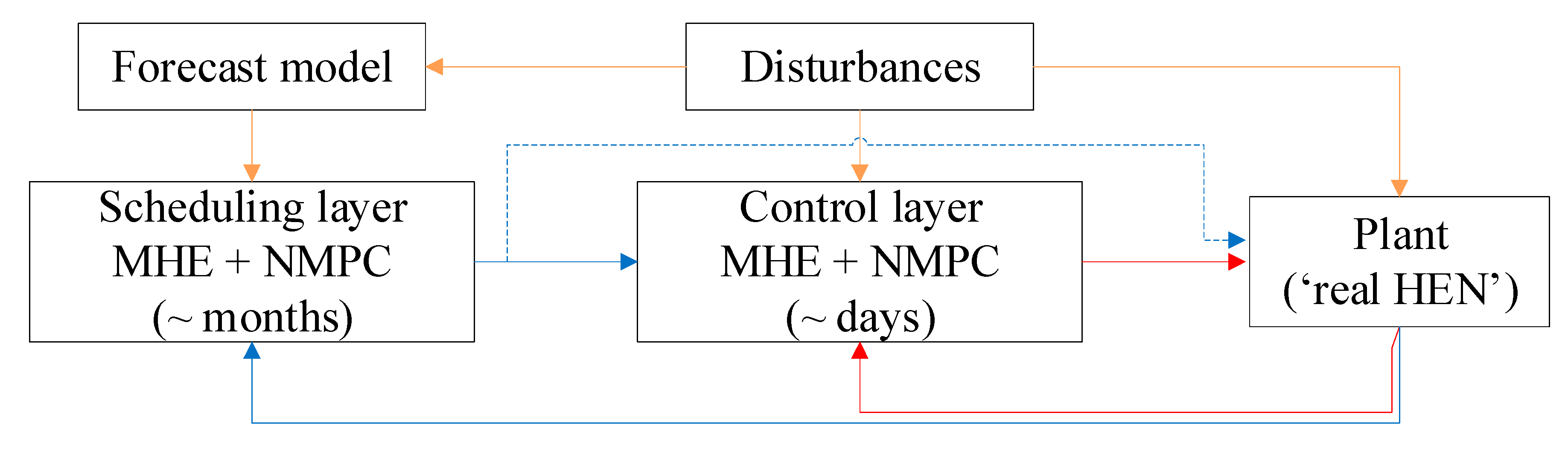
The online optimization approach of the cleaning schedule and dynamic flow distribution of preheat trains under fouling is based on an advanced nonlinear model predictive control (NMPC) strategy, presented in detail in a previous study by the authors [1]. It defines two feedback control loops, one for the fast dynamics of the process associated with flow distribution (of the order of hours) and another for the slow dynamics associated with fouling and cleaning (of the order of weeks and months). Figure 2 shows a simplified block diagram of the control loops, their components, and interactions. In this figure, the plant block corresponds to the actual system or a representation of it, the control layer refers to the advanced control and state estimator that defines the control elements of the system for rejection of fast disturbances (its inputs are the set schedule, the current state of the system, and disturbances, and the outputs are the control actions), and the scheduling layer refers to the algorithm defining the online scheduling strategy and its corresponding state estimator (its inputs are the current state of the system and a forecast of the disturbances, and the output is the schedule for the current time). Each control loop has two components: a moving horizon estimator (MHE) to update the model parameters and predict the current state of the system on the basis of the latest plant data and a nonlinear model predictive controller (NMPC) to optimize the future operation of the network. These two elements solve optimization problems using a realistically accurate and representative mechanistic, dynamic model of the plant. In particular, the model describes heat transfer, deposition rates, temperature changes, and hydraulic performance of the heat exchangers, as well as their interactions within the network that constitutes the preheat train. A brief, general description of the modeling components is given next, whereas a more detailed presentation of the model formulation and assumptions can be found in [16].
The preheat train model is based on a directed multigraph representation of the heat exchanger network, where each graph corresponds to a stream (e.g., crude oil, naphtha, residue) and the nodes are exchangers, furnace, sources, sinks, mixers, and splitters. At each node, mass and energy balances must be satisfied to ensure network connectivity. The operation of the heat exchangers, all assumed to be of shell and tube type, is represented using an axially lumped, but radially distributed model based on the P-NTU concept [28,29], an explicit description of the heat transfer and temperature profiles in the radial direction through different domains (shell, deposit layers, tube wall, tube), as well as hydraulic relations for the tube side pressure drop. The semiempirical reaction fouling model of Ebert–Panchal, Equation (1) [28], is used to characterize the evolution over time of the thermal resistance of the deposit in a unit. This affects the thermal performance of the unit and is related to the deposit thickness, Equation (2), affecting its hydraulic performance (all variables are defined in the Nomenclature). Experimental or plant data are required to estimate the parameters of the fouling model ). It has been demonstrated that this model adequately captures the main effect of the operating variables of the exchangers (e.g., surface temperature, velocity, shear stress) on the fouling rate [30]. In addition to these modeling components, operational limits such as the maximum duty of the furnace, the pressure drop limits in the network, bounds of flow split fractions to parallel branches, and pressure drop equalization constraints over parallel branches are included in the form of inequalities in the problem formulation. The resulting large set of nonlinear equality and inequality constraints is a sufficiently accurate [31] yet compact dynamic model of each exchanger and the network.
This dynamic model for preheat trains under fouling is used in the MHE and NMPC problems in both the scheduling and the control layers (labeled with subscript s and c, respectively) for parameter estimation, as well as to simultaneously optimize the flow distribution in the network and the cleaning schedule. It has been demonstrated, using actual refinery data, that this model has good predictive capabilities over a wide range of operating conditions and long operating times, with an average absolute prediction error in each exchanger of 0.9 °C for the tube-side exit temperature, 1.3 °C for the shell-side exit temperature, and 0.05 bar for the tube-side pressure drop [1].
Table 1 summarizes the main components, assumptions, and considerations of each feedback loop and their elements. In each layer, the MHE and NMPC formulations use the dynamic model described above to represent the operation of the preheat train and the effects of fouling. In the NMPC formulation of the scheduling layer, which includes binary decision variables, additional inequality constraints are included to represent the changes in operating modes of the exchangers (i.e., “operating” or “being cleaned”) and any conditions optionally imposed on the cleaning sequence (e.g., units to be simultaneously cleaned, periods of no cleanings, exclusive cleanings).
The control layer deals with the fast dynamics, and its main objective is to reject disturbances and minimize operating cost by manipulating flow split profiles, knowing the short-term cleaning schedule to be executed. The objective of the MHEC is to determine the model parameters that best explain the observations (i.e., temperature and pressure measurements from the plant) over a past estimation horizon, as represented in Equation (3). The adjustable parameters are the deposition and removal constants in the Ebert–Panchal model and the surface roughness, for each of the exchangers in the preheat train. The resulting formulation is an NLP problem. Once the MHEC problem is solved, the parameters thus obtained are used in the NMPCC problem (also formulated as an NLP) to determine the optimal flow distribution over a future prediction horizon that minimizes the operating cost, Equation (4). The latter includes the cost of the fuel consumed in the furnace and associated carbon emissions. The prediction time horizon is discretized using a discrete representation. Although the optimal solution covers a long horizon, only the first action is implemented in the plant; the remainder are discarded, and the problem is solved again in the next sampling interval, in the usual MPC scheme. The sampling (update) intervals are much shorter than the control prediction horizon. In this control layer, a forecast is required of the disturbances (changes in input variables) over the future prediction horizon. Here, each input variable (flowrate, temperature, and pressure of input streams) is forecast to remain constant at its last measured value for the entire horizon. As control updates are frequent, this is deemed to be adequate.
The scheduling layer deals with the slow dynamics of the process over long periods of operation. It integrates scheduling and control decisions to minimize the operating cost and to define the future cleaning actions. The MHES problem is similar to that of the control layer, and they share the same objective. However, the past estimation horizon of the scheduling layer is longer than in the control layer because more data is necessary to capture the slow dynamics of the system. On the other hand, the NMPCS problem is significantly different from that of the control layer. First, the future prediction horizon FPHS is much longer, as it must be able to schedule cleaning actions and quantify their effects and benefits. Second, the objective function includes both operating cost and cleaning cost, Equation (5). Third, the prediction time horizon is here discretized using a continuous rather than a discrete representation, to reduce the number of binary variables of the scheduling problem. Each period of variable length is further discretized using orthogonal collocation on finite elements in order to accurately integrate the differential equations in the model. Fourth, in this scheduling layer, a forecast is also required of the disturbances over the future prediction horizon. Here, each input stream variable (flowrate, temperature, and pressure) is forecast to remain constant for the entire horizon, but fixed at the value of its moving average over the past month, to account for recent variability. Alternative forecasting estimates (e.g., reflecting predicted trends or known planned changes) could be used. Lastly, the optimization problem involves binary decision variables associated with the operating mode of the units at every time point, resulting in an MINLP instead of an NLP formulation. This is a challenging optimization problem because of the large number of binary variables, few constraints on the cleaning sequence, nonlinearities, nonconvexities, and the degeneracy of the objective function (i.e., multiple solutions may have similar values). To solve the MINLP problem that integrates cleaning scheduling and flow control, a reformulation using complementarity constraints is implemented, which allows finding local optimal solutions online in reasonable computational times [32].
The scheduling layer is not updated as frequently as the control layer because of the different time scales involved. However, the two layers interact strongly so as to ensure that scheduling and control decisions are properly integrated and their synergies exploited. The optimal scheduling actions determined at the scheduling layer until the next schedule update are executed in the plant. They are also sent to the control layer, which determines the best flow distribution according to those cleanings and the disturbances observed. Other schedule decisions in the schedule prediction horizon beyond this first interval are discarded.
For the purpose of this paper, the actual plant is simulated using the same predictive model as used in the NMPC/MEH loops. However, its parameters are modified in order to create a controlled degree of (parametric) model mismatch. The plant parameters are unknown to the feedback loops.
3. Closed-Loop Schedule Stability Metrics
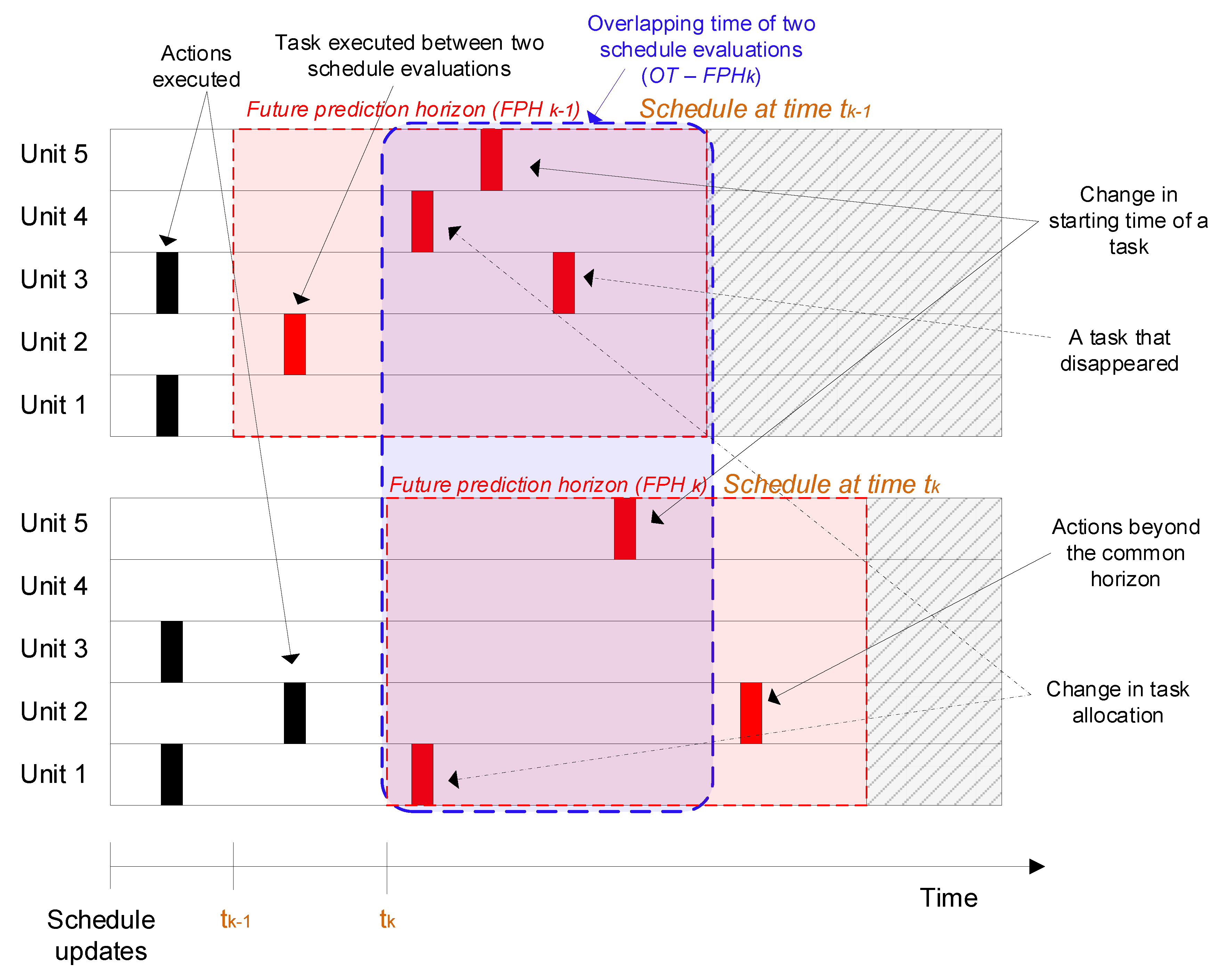
Closed-loop schedule instability must be quantified to determine efficient strategies to reduce it, but no single metric is adequate. In production scheduling, it has been quantified as the difference in the overall quantity of a given product produced at a given time between two consecutive evaluations of the schedule [33]. Other attempts have quantified the changes in starting time of the same task between two consecutive solutions [34] or the changes in task allocations among the units [34,35]. Reference [30] considered batch plants; thus, their criterion is not immediately applicable to the problem of interest here, which is a type of maintenance scheduling for a continuous process. An analogous concept will be developed later which is applicable to continuous processes. On the other hand, the differences in the starting time of tasks (the cleanings) and in the task allocations (which exchanger is cleaned and number of cleanings per exchanger) will be used to quantify schedule instability, according to the notation in Figure 3.The figure shows the cleaning schedules for a five exchanger network at two consecutive evaluations (at the top, schedule k − 1 evaluated at time ; at the bottom schedule k, evaluated at time ) and a representation of the main schedule differences, including changes in task allocations (which units are cleaned) and the starting time of the tasks (when cleanings start). The schedule instability is defined taking into account those actions within the overlapping interval, OI, in the future prediction horizons of the two consecutive schedules. With constant schedule update interval and length of the scheduling prediction horizon,, the duration of this overlapping interval is also constant and simply equal to their difference, − . With variable intervals, the same definitions are indexed according to the schedule evaluation index, k, i.e., the overlapping interval at evaluation k, has duration − .
Four metrics of schedule instability are defined next on the basis of these definitions: (1) task time instability, (2) task allocation instability, (3) overall instability, and (4) overall weighted instability. They are defined for consecutive schedule evaluations assuming a continuous time representation, although they also apply with a discrete time representation. Instability metrics are generated every time a schedule is updated, and, in an online application, their time evolution can be tracked on a rolling horizon at each update.
The metrics defined here can provide useful insights into schedule stability regardless of how the schedule is defined. The only condition for their application is the existence of two consecutive evaluations or predictions of the schedule with a common period. The definition of these metrics is based on the changes occurring within a common period shared by the schedule evaluations. Hence, these metrics can be calculated for two consecutive instances even in cases where their control horizons, scheduling horizons, or update frequencies are different.
The following definitions, sets, and indices are used to define the instability metrics for the online scheduling problem:
- . Set of units.
- . Set of tasks that can be allocated to the units.
- . Set representing time in the .
- . Set of schedules evaluated over time.
- . Binary variable indicating the allocation of a task to a unit starting at a time in schedule .
- . Time when schedule is evaluated.
- . Time interval between two consecutive schedule evaluations.
- . Set of the starting times of all tasks allocated to unit in schedule and within the time interval .
- . Set of the starting times of all tasks allocated to unit in a schedule evaluation and within the operating interval .
- . Set assigned to or based on which one has the minimum number of elements.
- . Set defined as the complement of .
Although, in this paper, fixed update intervals are used, the formulation is suitable for both fixed and variable update intervals.
For the application at hand, i.e., cleaning scheduling of preheat trains under fouling, it is assumed that only one type of cleaning is available (i.e., mechanical cleaning) so that the set Tasks has a single element, i.e., {1}. Moreover, the set Units is the set of heat exchanges in the network, and the variable defined here has the same role as variable in the problem formulation detailed in [16], which is associated with the cleaning state of the units over time (i.e., 1 for being cleaned, 0 for operating). In this formulation, it is possible to assign multiple mechanical cleanings (i.e., multiple instance of the same type of task) to a unit, at different times.
As the (in)stability of a schedule is a relative concept (i.e., it only applies with reference to a previous one), all metrics apply from the second evaluation only (k ≥ 2) and are undefined (and arbitrarily set to 0) for k = 1.
3.1. Task Timing Instability
A Task timing instability of schedule , , is defined as the difference in the starting times of all tasks in units which are common to schedules and over the overlapping interval, . Its mathematical representation is presented in Equation (6). Note that this includes only tasks j that are defined in both schedules and . If multiple executions of task are included over in both schedules, the difference in their starting times is only relevant for the minimum number of instances of task predicted in either one. In addition, if in schedule , or , there are no predicted executions of task in unit , there is no contribution of this task-unit pair to the overall task timing instability metric.
This instability metric is divided by the future prediction horizon of the scheduling problem at update , , to transform it into a dimensionless quantity. The task timing instability takes a value of zero when there is no difference in the predicted starting time of all the common tasks allocated to all the units in two consecutive schedule evaluations, or when no task of the same type is allocated to the same unit in two consecutive schedules (i.e., all the tasks allocated to a unit disappeared from the schedule or were reallocated to another unit). The task timing instability increases when the difference in the starting times of a task allocated to a unit in two successive schedules is large.
3.2. Task Allocation Instability
A Task allocation instability of schedule , , is defined as the change in the total number of executions of tasks allocated to unit in schedule k during the , with respect to the total number of executions of the same task in the same unit in the previous schedule, . This is expressed mathematically in Equation (7). This expression assumes that all tasks have the same relative importance for the stability and only considers their total number of executions. In the cleaning scheduling application considered, this refers to the change in the total number of cleanings of each exchanger within , regardless of their starting time.
This definition of instability is standardized by dividing it by the sum of the maximum number of executions of task that are allowed in unit , .This is a parameter of the scheduling problem, and is specified by the analyst. For example, in the cleaning scheduling problem of preheat trains under fouling, it is the maximum number of cleanings per exchanger that can be executed in the future prediction horizon, which is usually a constraint imposed by the operators.
The task allocation instability becomes zero when there are no changes in the number of tasks of a given type scheduled in each unit regardless of their starting time or when there are no tasks of a given type scheduled in the future prediction horizon. This instability metric increases when one or more instances of a task are added to or deleted from one or multiple units in the current schedule with respect to the previous one.
3.3. Overall Schedule Instability
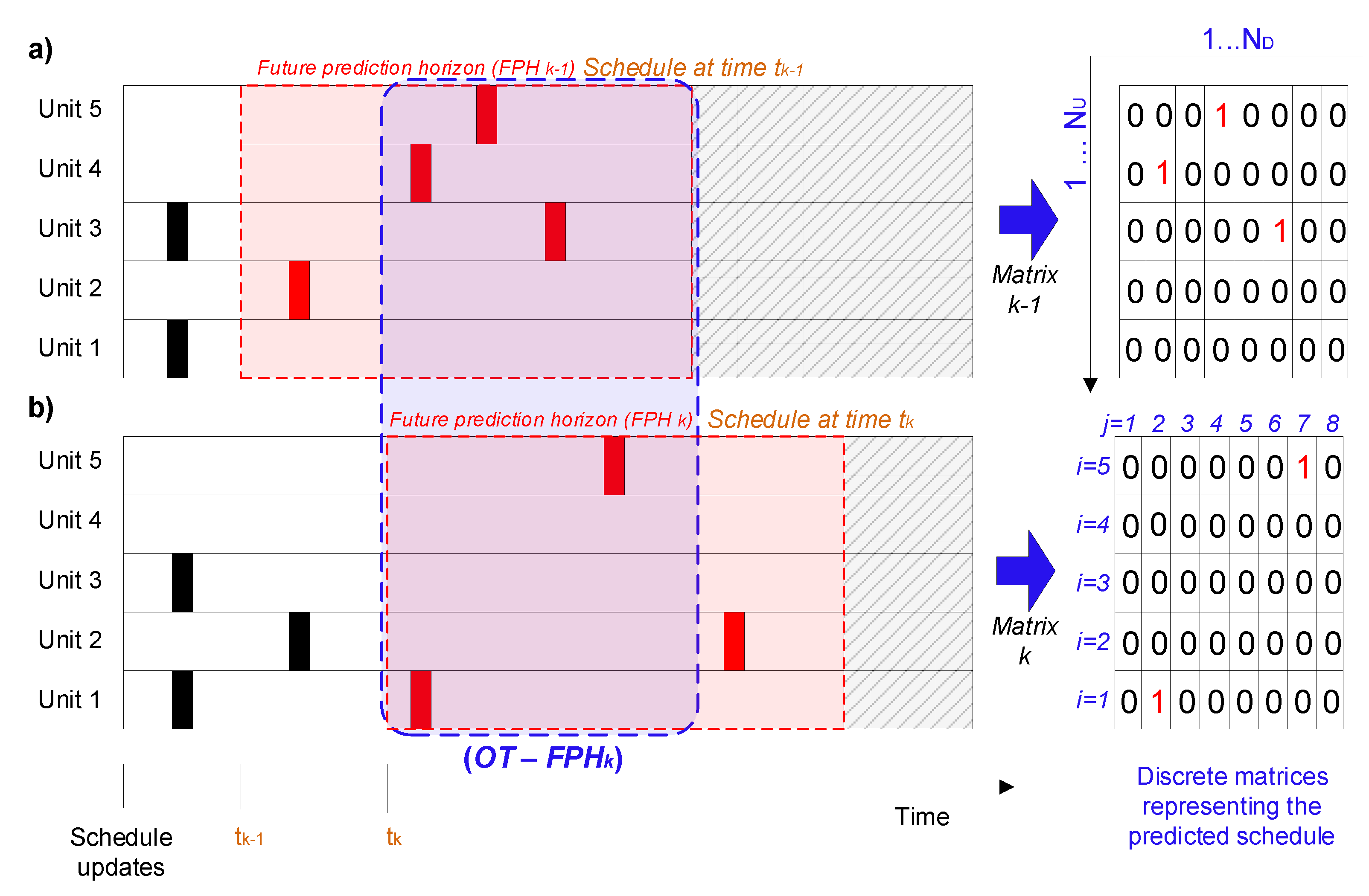
A metric of Overall schedule instability of schedule , should consider all the changes from the previous schedule k − 1, such as changes in the starting time of the tasks, changes in task allocation, addition of new tasks, and disappearance of previous tasks. To compute it, the overlapping interval is discretized using a time step that is lower than or equal to the shortest duration of any of the tasks present in either schedule. In the case of preheat trains, the sampling time of the process is used, which is 1 day, as plant measurements are available as daily averages. With this time discretization, a schedule matrix is defined representing a schedule, with rows, one per each unit, and columns, each representing a snapshot of the tasks scheduled at each time step during the . Each element of the schedule matrix is referred to as x(i,j,k) where i is an index for the units (rows), j is an index for the time instances in the discretized (columns), and k is the schedule index. The entries in the matrix are either 0, representing no task allocated, or 1, representing a task allocation. This definition assumes that there is a single task type to be scheduled, as applicable to the single type of cleaning in the scheduling of preheat trains discussed in this paper. However, it can be easily extended to a more general formulation with multiple tasks, by associating different integer values to each task type or different instability metrics for each task.
Figure 4 illustrates such a schedule matrix encoding for a simple example for schedule k − 1 evaluated at time (top schedule in Figure 4) and schedule k, evaluated at time (bottom schedule in Figure 4). The corresponding schedule matrices (on the right in Figure 4) have the same dimensions because , the sampling time, and the number of units do not change between evaluations. With this encoding, it is possible to rapidly calculate the difference between two successive schedules on the basis of the differences in individual elements of the corresponding schedule matrices.
The Overall schedule instability of schedule , , is defined in Equation (8), where the quadratic difference between two consecutive schedule matrices, and , is calculated element by element, and all the differences are added up. This instability metric is standardized by dividing it by the size of the schedule matrix (). All schedule changes are assumed to have the same effect on the overall schedule instability metric. They affect it by the same magnitude and do not differentiate between schedule differences due to changes in the starting time of the tasks, time delays, or changes in task allocations. Because this metric is standardized, it is bound between zero and one and increases with the number of differences between consecutive schedule evaluations.
In the example presented in Figure 4, there are five changes in the schedule matrices between schedules and (see columns 2, 4, 6, and 7 of the matrices in the figure). Then, applying Equation (8), the overall schedule instability of schedule k is 0.125.
3.4. Time-Weighted Overall Schedule Instability
The above Overall schedule instability definition ignores when the difference in the schedules occurs. For example, the values of the overall schedule instability for two different schedules can be the same when changes in the schedule are observed at the beginning of the , which has large implications on the operation because those are the actions to be executed in the current time step, or at the end of the , when they may not be very important and are subject to future changes. The metric described below addresses the case when changes in the schedule closer to the current execution time are undesirable.
A Time-weighted overall schedule instability metric of schedule , , is defined in Equation (9), where weights are used to represent the relative importance of each difference in the schedules with respect to time. This expression uses the same definitions of overall schedule instability, Equation (8), which are based on a matrix representation of the schedule over . Here, the weights are selected to decrease linearly from one at the beginning of the overlapping interval , to zero at is end, according to Equation (10). In terms of the discretizations used in the schedule matrix, we have for and for . The differences in the schedules closer to the current time are, thus, given a higher relative importance than those that occurring later in the prediction horizon.
Using weights to characterize the relative importance changes in the schedule with respect to time was proposed to calculate schedule instability on the basis of the production quantity of different products [33,36], but not for differences in task allocation and timing. Those studies used an exponential decay function to define the weights as a function of time. This could also be used here without adding complexity to the problem. The only difference is that the exponential decay function requires the analysts to set a parameter for the rate of decay, which can be translated as a preference to ignore or not schedule modifications occurring at a future time.
The time-weighted overall schedule instability metric explicitly accounts for the effects of time to indicate that large variability close to the current time is undesirable, whereas that occurring later can be tolerable. However, it does not distinguish whether the source of variability is due to changes in the task allocation or starting time of the task.
Applying the metric defined in Equation (9), the time-weighted overall schedule instability of schedule k in Figure 4 is 0.136, which is higher than its overall schedule instability, 0.125. This happens because most of the differences between the two consecutive schedules occurs close to the current time, , which is reflected in a larger number of differences between the schedule matrices in columns with low indices (columns 2 and 4 of the matrices in Figure 4). This example shows that the time-weighted metric gives more importance to changes in the schedule that occur closer to the current time and that may require an immediate action.
4. Including Stability Considerations in the Online Optimization Problem
There are various alternatives to improve the closed-loop stability of online scheduling, but their actual benefits are not clear, nor is their effect on the overall economics of the process. Three alternatives based on MPC theory and their practical implementation are evaluated here. They are (1) introducing a terminal cost penalty with respect to a steady state in the objective function, (2) freezing or fixing a subset of the scheduling decisions in the in consecutive schedules, and (3) penalizing changes in scheduling decisions between consecutive evaluations. These alternatives are described next in the context of online cleaning scheduling of preheat trains under fouling.
4.1. Terminal Cost Penalty
In MPC for continuous systems, the closed-loop stability properties have been widely studied from practical and theoretical perspectives (as noted below, the stability definition for continuous control is different from the schedule stability used in this paper). One alternative to ensure closed-loop stability with a finite prediction horizon is to include a “terminal cost” in the objective function of the optimization problem solved at every sampling time [37] in the form of Equation (11). This represents a general objective function, where are continuous variables, are integer variables, and are manipulated variables, which are minimized in an MPC scheme at each sampling time. The function is the “running cost”, which, in tracking problems, is defined as the quadratic difference between the states and their reference point. The function is the “terminal cost”, and it is only a function of the variables at the end of the prediction horizon, (for example, the cost of missing a final target). The parameter represents a penalty on the terminal cost and indicates its relative importance with respect to the running cost.
In our case, the overall integral of the running cost, , in Equation (11) is just the total operating cost of the preheat train (i.e., the objective function of the online scheduling problem, defined in Equation (5). There are, however, important differences between the general MPC formulation and that for closed-loop scheduling that hinder the applicability of adding a “terminal cost” to improve stability. First, the assumptions to guarantee stability in MPC state that the objective function must decrease with the number instances evaluated; however, in the case of closed-loop scheduling, the objective is economic, and this assumption may be violated. Second, the scheduling stability problem is nonconvex and nonlinear; thus, global optimality cannot be guaranteed. Third, the maintenance/cleaning scheduling problem considered does not have an obvious stable reference point to use in a tracking function. The clean state of the network (ideal) is not achievable without infinite cleanings. A possible reference for the problem on hand is proposed below. Fourth, the scheduling problem includes discrete variables over a long time scale instead of continuous variables over short time scales. Lastly, stability for MPC is defined according to whether the system remains in the same operating point (outputs of the plant) regardless of small disturbances [37], while, for closed-loop scheduling, stability is defined as a function of the intensity of the changes in scheduling variables (inputs to the plant) between consecutive solutions.
Here, according to the rationale to avoid leaving the network unnecessarily clean at the end of the scheduling horizon, the reference point for use in the terminal cost is defined as the operation where each exchanger has reached its asymptotic or maximum fouling level or an operational constraint has been reached. This limit operation is determined by performing a simulation of the system, assuming average operating conditions and no mitigation actions. Alternatively, a stable reference operating point could be defined on the basis of engineering judgement (i.e., a realistic, possible operating state expected or observed in the past). Other scheduling problems may have cyclic solutions that can be used as references for stability [38]. The terminal cost for the online optimization of flow distribution and cleaning schedule is defined in Equation (12), as the sum for all streams in the network of the quadratic difference between the stream temperature predicted at the end of the , , and the corresponding one in the limit operation, The set Arcs in Equation (12) is the set of all arcs (streams) in the network.
4.2. Freezing Decisions
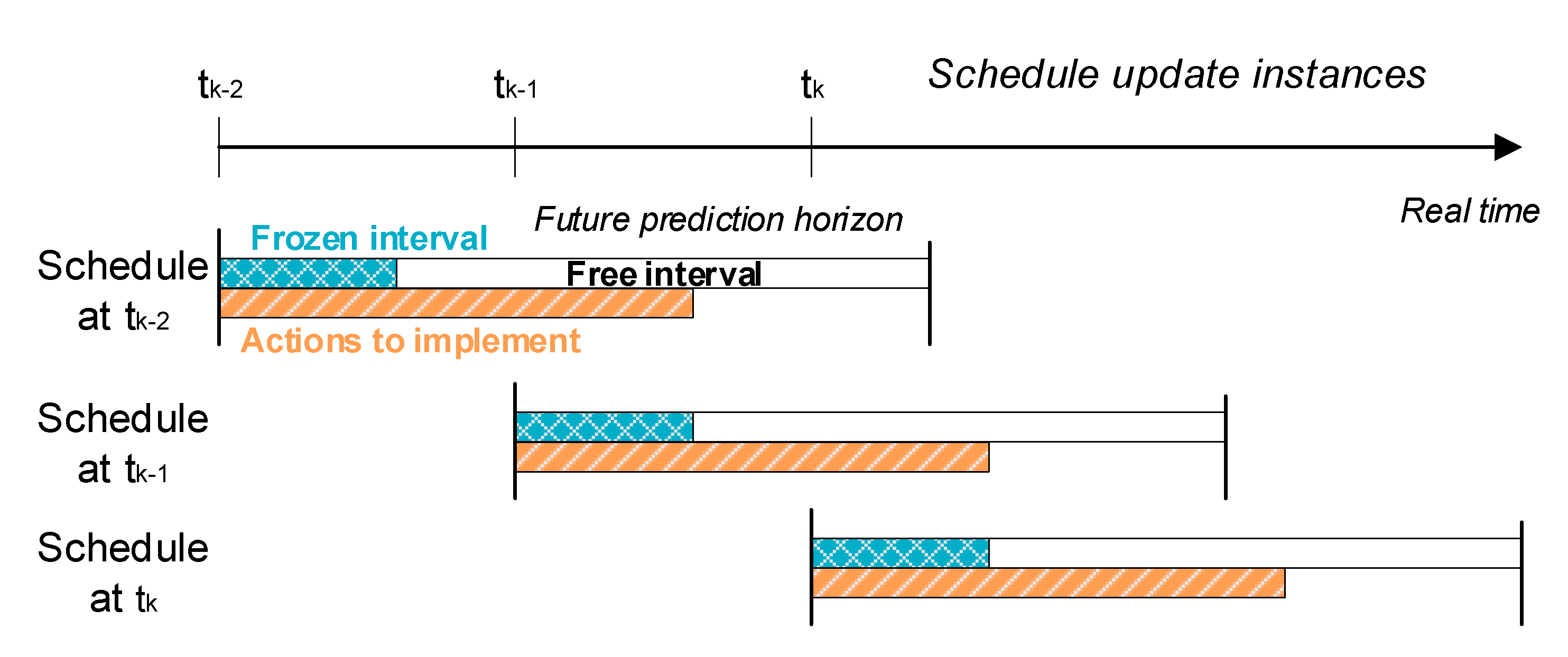
Fixing or freezing some of the scheduling decisions within the prediction horizon, i.e., retaining those of a previous schedule, explicitly reduces scheduling instability [39,40]. Every time a scheduling problem is solved, a fraction of the decisions from the previous schedule evaluation are frozen, and the remainder are considered free. The fixed actions are defined as equality constraints in the next scheduling optimization problem. The time intervals for online scheduling and the nature of the decisions at each evaluation are schematically shown in Figure 5 for three successive updates. The actions executed between sampling times are a mix of those frozen from the previous solution and those obtained at the current evaluation. The length of the frozen interval and the scheduling decisions included, such as task allocated and starting time of the tasks, give a trade-off between stability and closed-loop performance.
In the online cleaning scheduling and flow distribution problem of preheat trains, there are two kind of decisions that can be kept constant between consecutive schedule updates: the assignment of cleanings to periods and units and the starting time of the cleaning actions. Equality constraints are introduced to fix the selected cleaning actions in the current schedule to the values calculated in the previous one. Equation (13) shows this constraint for the binary decisions, where the asterisk denotes the optimal value in the previous schedule. These equality constraints assign the cleanings to the units and periods; however, because the periods have variable length (with a continuous time representation), the starting time of the cleanings is not fixed. To allow more flexibility, inequality constraints are introduced to restrict the variability of the cleaning starting time with respect to that of the previous optimal schedule. This is shown in Equation (14) which can be transformed into an equality constraint if necessary.
4.3. Penalizing Variability
Penalizing the change in scheduling decisions between two consecutive evaluations is another alternative to improve closed-loop schedule stability. Instead of using constraints to reduce the variability between consecutive schedule evaluations, the variability is penalized in the objective function. The changes between two schedules are only penalized within their overlapping horizon , as detailed in Figure 3.
The schedule variability penalty is divided into two independent terms: one for the changes in the allocation of tasks, Equation (15), which is related to the task allocation instability metric, and another for the changes in the starting time of the tasks, Equation (16), which is related to the task timing instability metric. Each of these expressions has a penalty parameter that characterizes its importance relative to the other and to the economic objective function of the scheduling problem. The final overall objective function for each schedule update, Equation (17), shows the compromise between stability and process economics. As noted, the integral of the running cost, V, is the total operating cost of the preheat train, which is the objective function defined in Equation (5).
5. Comparing Alternatives and Metrics to Improve Closed-Loop Schedule Stability
This section evaluates all the instability mitigation approaches presented in Section 4 that utilse the metrics in Section 3 for a simple, yet realistic, case study.
5.1. Case Study 1—Illustrative Example
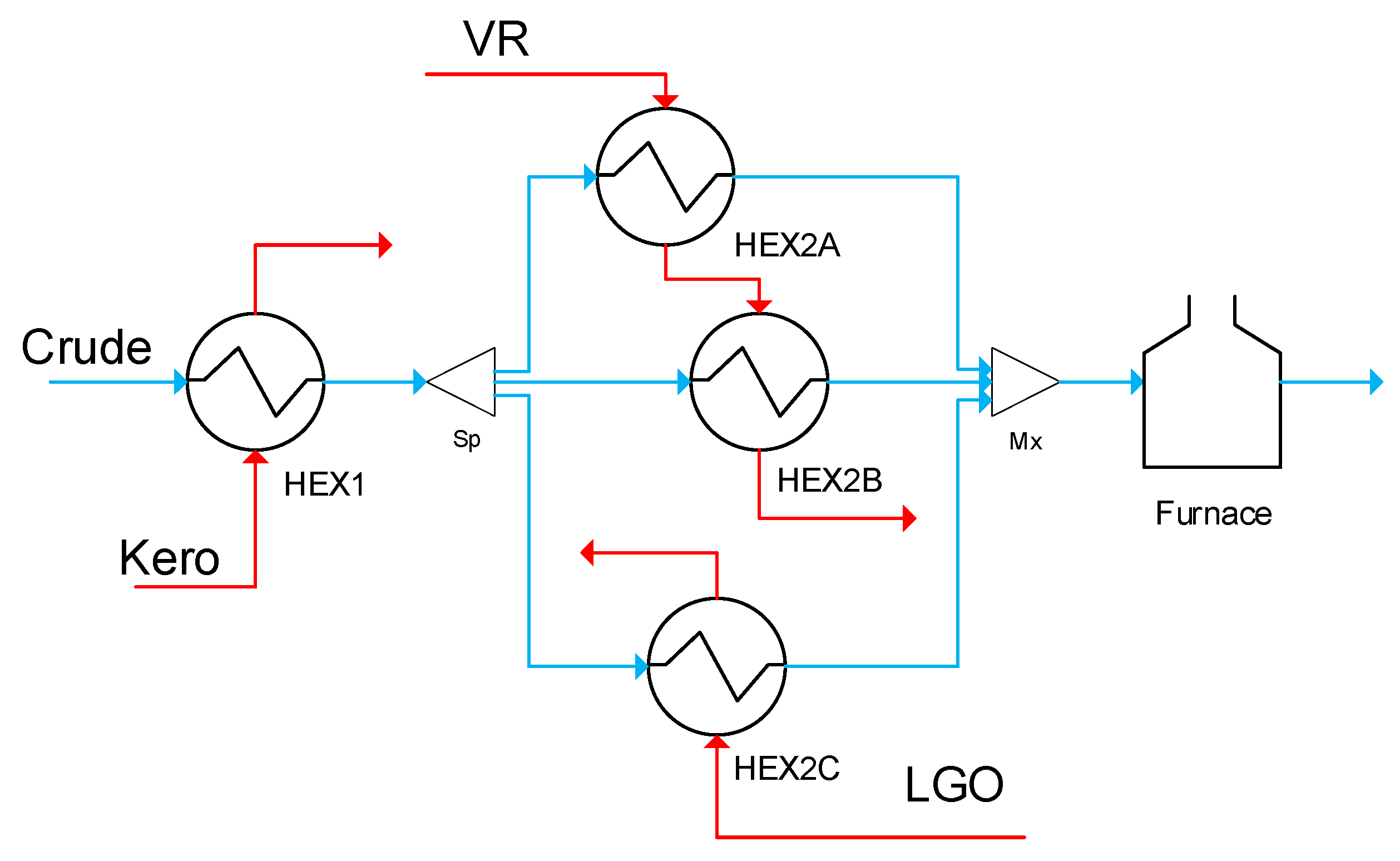
The preheat train considered here consist of four heat exchangers, three of which are located on parallel branches. This case study was adapted from [41,42], where all the details of the equipment, costs, and operation can be found, although the most important ones, including the fouling model and cost parameters, are summarized in Table A1 and Table A3 (Appendix A). Figure 6 shows the structure of the network, which is commonly found in refining operations with more units in the branches. All exchangers are shell and tube and exhibit significant levels of fouling.
For this case study, a nominal operation was assumed (i.e., with constant inlet streams flow rates and temperatures) with no model–plant mismatch; thus, the predictive models used in the feedback loops perfectly represent the plant. These assumptions lead to a simpler problem than a real application of the online approach, while they allow isolating the analysis of the stability of the online scheduling from other aspects. This case also demonstrates that there can be schedule instability even under these ideal conditions.
5.2. Results and Discussion
The online optimal control and cleaning scheduling problem was solved with the following settings: for the control layer, a control horizon of 10 days and update intervals of one day; for the scheduling layer, a scheduling horizon of 120 days, update intervals of 15 days, and 15 periods of variable length in the scheduling horizon. The MHE problems were not solved in the feedback loops because there is no plant–model mismatch. These settings of the closed-loop scheme led to 25 solutions of the optimal cleaning scheduling problem over 1 year of operation. The schedules obtained were used to calculate the schedule instability metrics for 24 consecutive solutions after the first one.
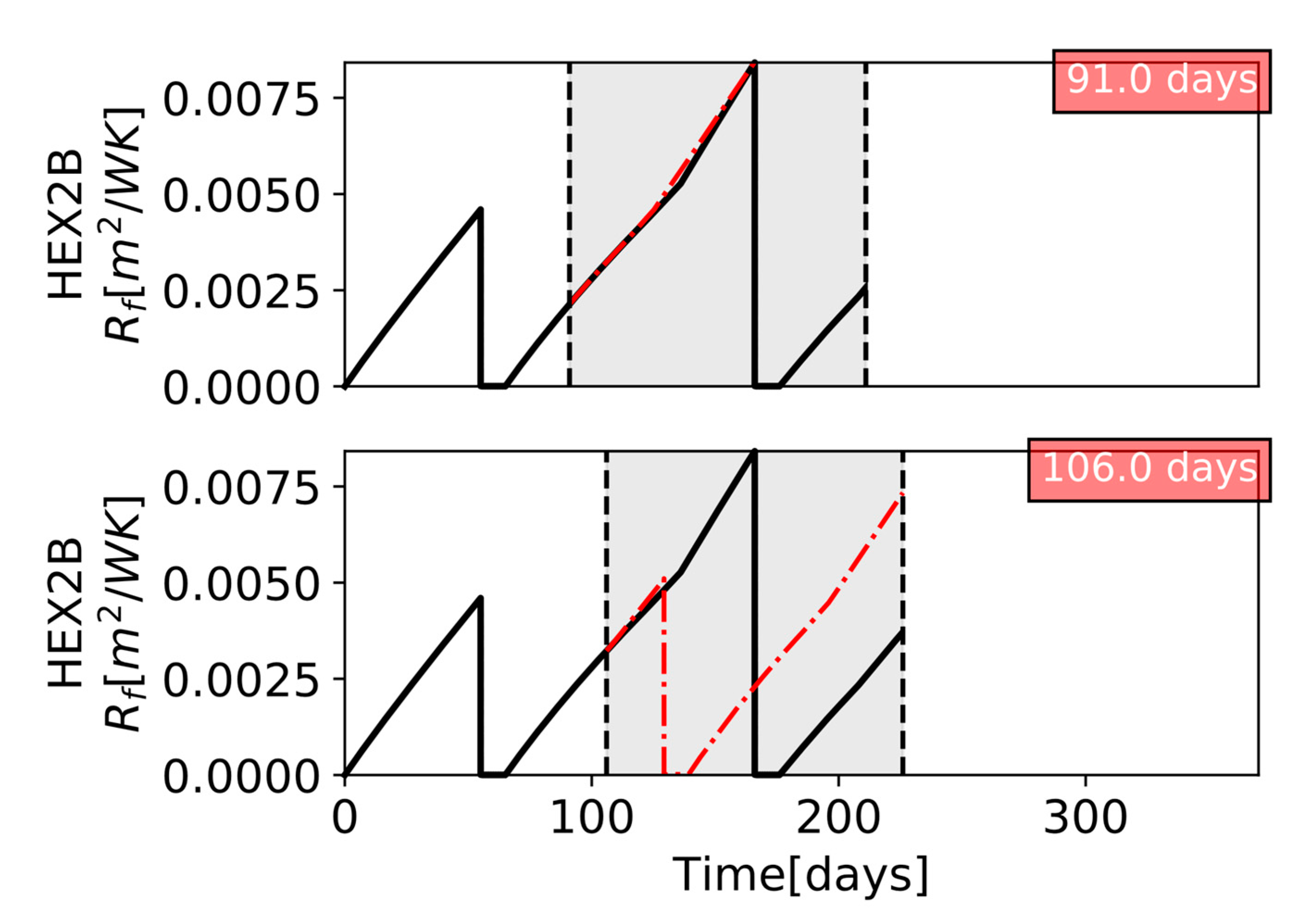
The closed-loop optimization was first performed with the usual economic objective function without including stability (base case). An example of changes in schedule between successive updates is shown in Figure 7 with reference to the predicted fouling state (in terms of fouling resistance) of exchanger HEX2B. At the update on day 91, no cleanings of HEX2B were scheduled over the predicted horizon (red line in Figure 7, top). At the day 106 update, a cleaning was introduced, scheduled for day 120 (red line in Figure 7, bottom). Due to intervening variations in the plant, the cleaning was eventually shifted and executed on day 170 (black line in Figure 7).
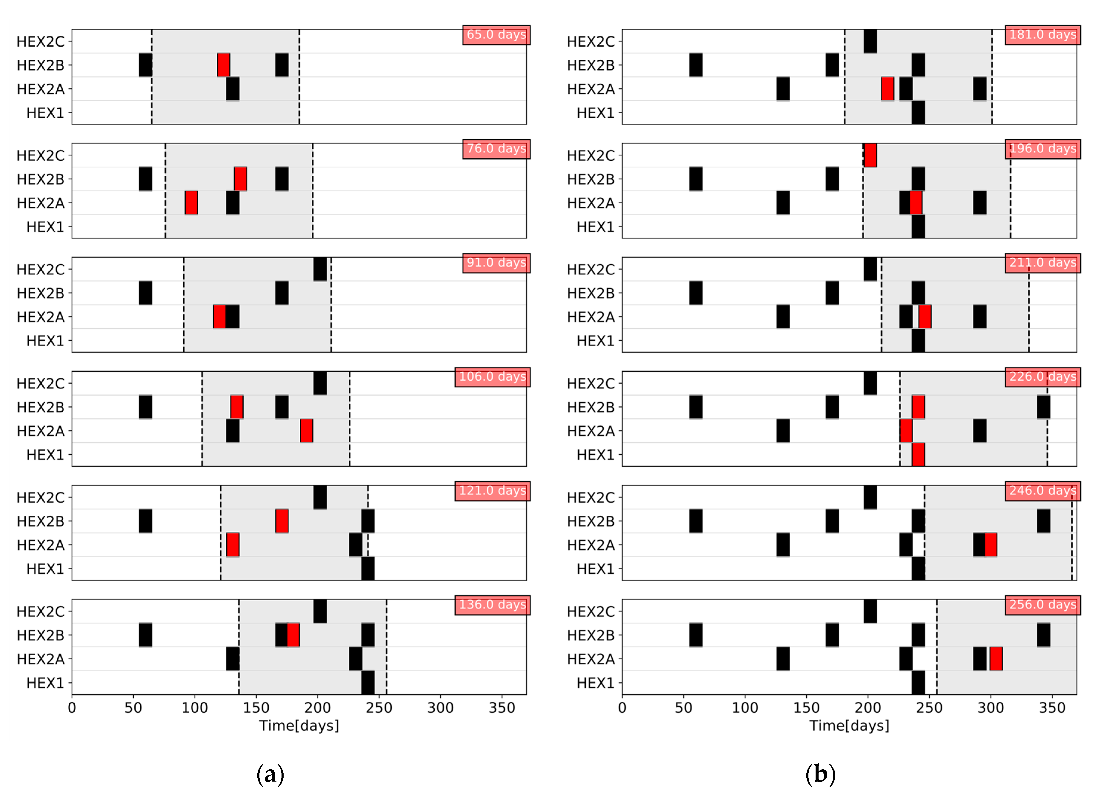
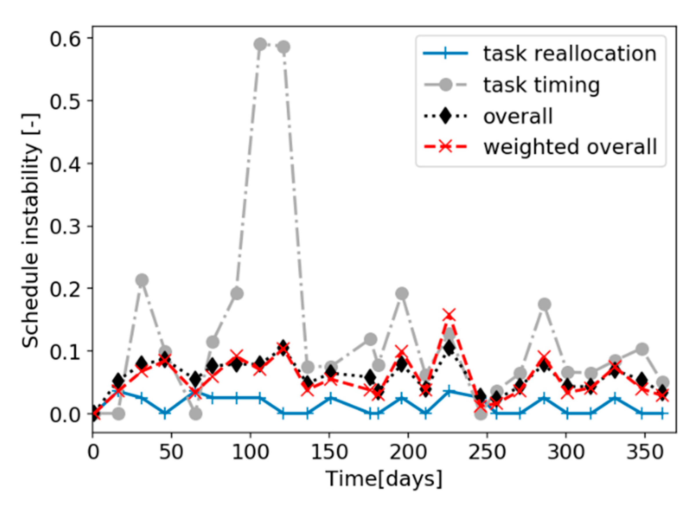
Figure 8 presents the cleaning schedule predicted (red) at six successive sampling times each over two time windows, together with the schedules eventually executed over the entire horizon (black). Figure 9 shows the schedule instability metrics calculated at every cleaning schedule update. In all updates, there are some changes in the optimal cleaning schedule with respect to the previous one, and this is reflected in the evolution of the instability metrics. The peaks of task timing instability occur when a cleaning was postponed, and the task allocation instability changes when cleanings are included or removed from the predicted schedule. The overall instability and the time weighted overall instability are good single indicators of instability as their behavior aligned with that of the other metrics.
The variation in scheduling instability metrics observed in Figure 9 can be explained by the evolution of the cleaning schedule. For instance, the maximum value of task timing instability is observed between 90 and 120 days of the operation because the starting time of the cleanings predicted for HEX2A and HEX2B change significantly, and even their precedence order is reversed. As another example, between the schedule evaluations at 65 days and 76 days, there is one additional cleaning introduced, causing an increase in the task allocation instability. The final example relates to the overall instability and the time-weighted overall instability metrics. Consider the consecutive schedule solutions at 211 and 226 days, when two new cleanings are predicted and the starting time of the HEX2A cleaning are shifted closer to the current time. The weighted overall instability metric is higher than the overall instability because all the changes occur closer to the execution time.
Next, the three alternatives proposed in Section 4 to improve closed-loop scheduling stability were implemented, with the parameters varied as follows:
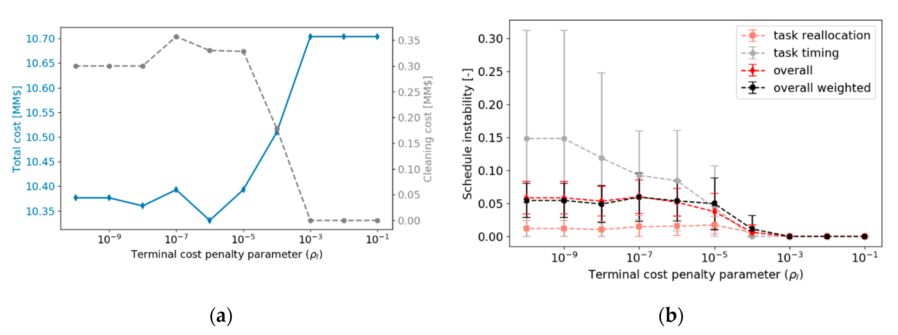
- In the terminal cost penalty (Equation (12)), was varied between and on a logarithmic scale.
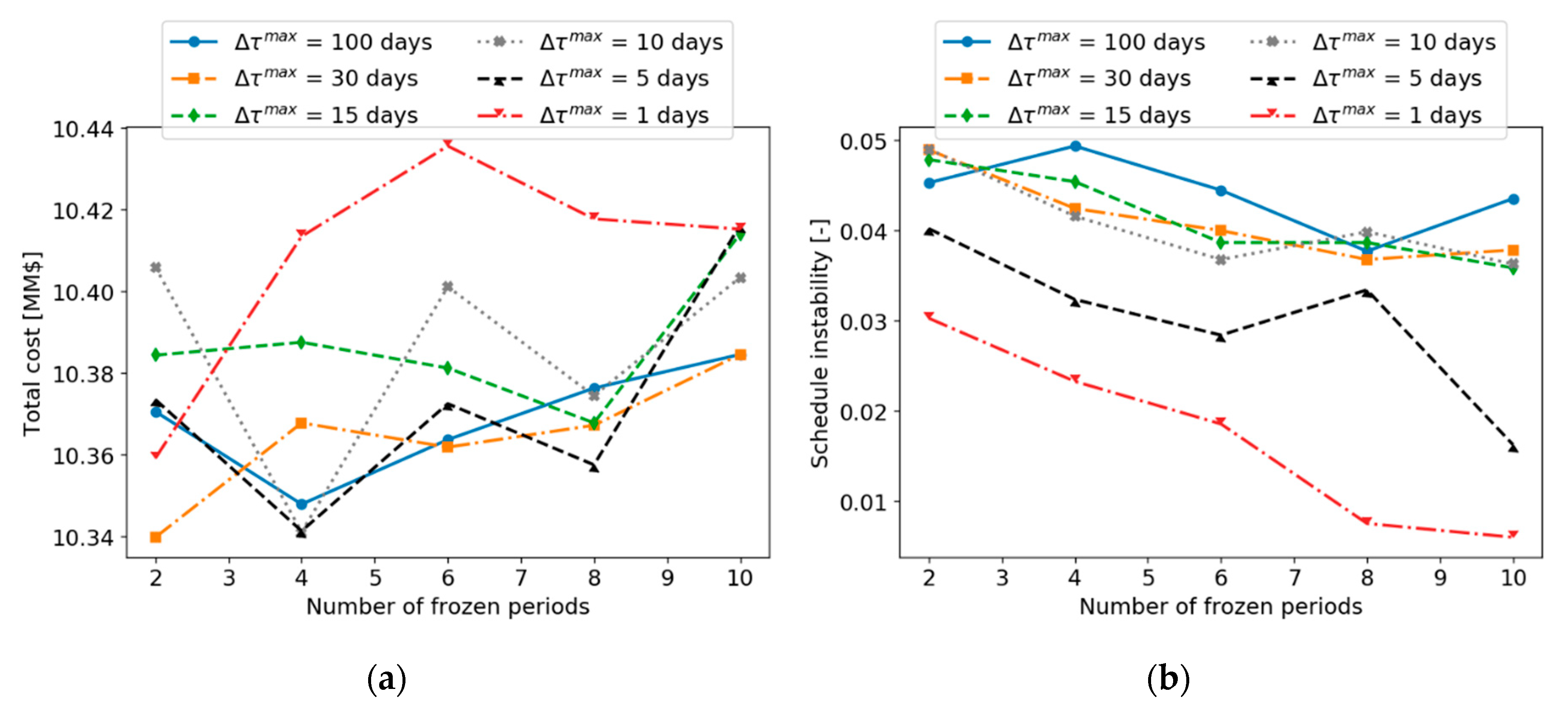
- In the freezing horizon alternative (Equation (14)), the number of periods in which decisions are kept constant, , was varied between 2 and 10, and the maximum allowed variation in the cleaning starting time, , was varied between 1 day and 100 days.
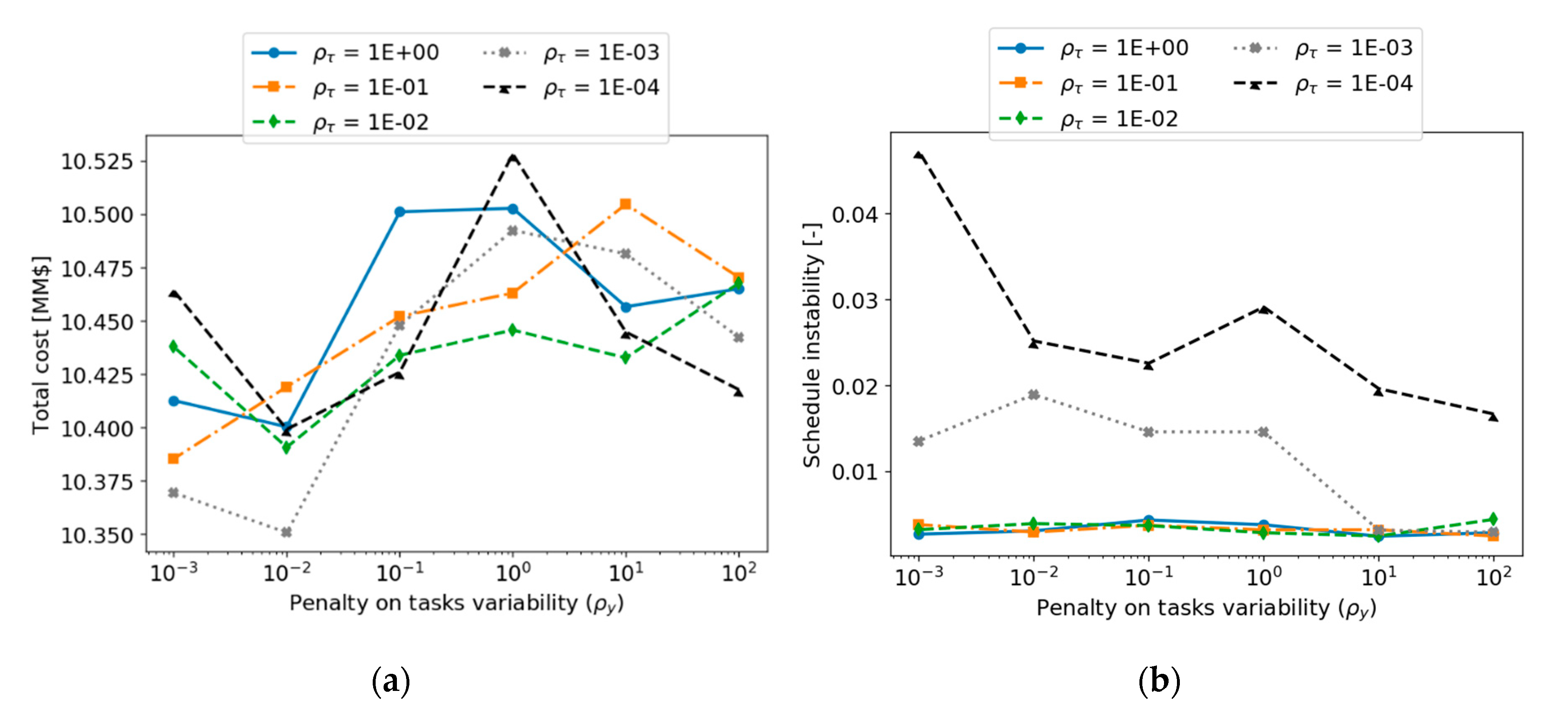
- In the variability penalty alternative (Equations (15)–(17)), the penalty parameter of the cleaning allocation variability, , was evaluated between and , while the penalty parameter of the cleaning starting time variability, , was varied between and . The different ranges were due to the differences in the order of magnitude of the metrics.
Figure 10 shows the closed-loop economic performance and stability metrics obtained when using the terminal cost alternative to reduce instability, for various values of the penalty parameters. The bars in Figure 10b represent the standard deviation of each metric. Increasing the terminal cost penalty improves the schedule stability but increases the operating cost. At the upper value of the terminal cost penalty, , the closed-loop solution has no cleanings scheduled over the entire horizon. This is the most stable solution, but also the most costly. Low penalties reduce the total operating cost as they allow more variability and a higher reactivity in the scheduling actions. For terminal cost penalties lower than , the total operating cost and the average of most instability metrics do not change significantly, but the task timing instability changes. When large variability in the scheduling decisions is allowed (low penalties), the effect of changes in the starting time of the cleanings dominates over that of the assignment of cleanings to units. The results show that proposed metrics may be used as good indicators of the overall closed-loop schedule stability.
Figure 11 illustrates the effect of freezing some scheduling decisions beyond the scheduling sampling time. It shows the total cost and the average of the overall weighted schedule instability as a function of the number of periods frozen and the maximum change allowed in the starting time of cleanings (for clarity, only the average value is shown without indicating its variability). Only the overall weighted instability is used from now on as it is the most comprehensive and illustrative metric among those proposed. The total operating cost increases with the number of periods frozen, while the schedule instability decreases, although no clear trend is observed, as the nonlinearities, nonconvexities, and combinatorial nature of the problem potentially lead to local optimal solutions. A higher number of periods frozen results in fewer degrees of freedom in the scheduling problem, limiting the opportunity to react optimally. When the range of changes in the cleaning starting time is also restricted, it is observed that, for low values of this bound, the closed-loop schedule is more stable than for high values, and its total operating cost is higher. For a cleaning starting time variability bound greater than 10 days, there is no significant change in the schedule stability, but the operating cost varies. In these scenarios, the total number of cleanings and their allocations have a higher impact on the process economics than their starting time.
For the variability penalty alternative, which penalizes changes between consecutive schedules, Figure 12 presents the effect of its parameters on the closed-loop performance and schedule stability. Although no clear trend is observed, the total operating cost increases when the penalties on the variability are higher, while the schedule instability decreases. For values of lower than the schedule instability values did not change, but the operating cost could still vary, indicating that the effect of cleaning starting times is not as significant as the cleaning allocation. Furthermore, the two penalties in this alternative are correlated, and there are different combinations leading to similar closed-loop performance of the overall system.
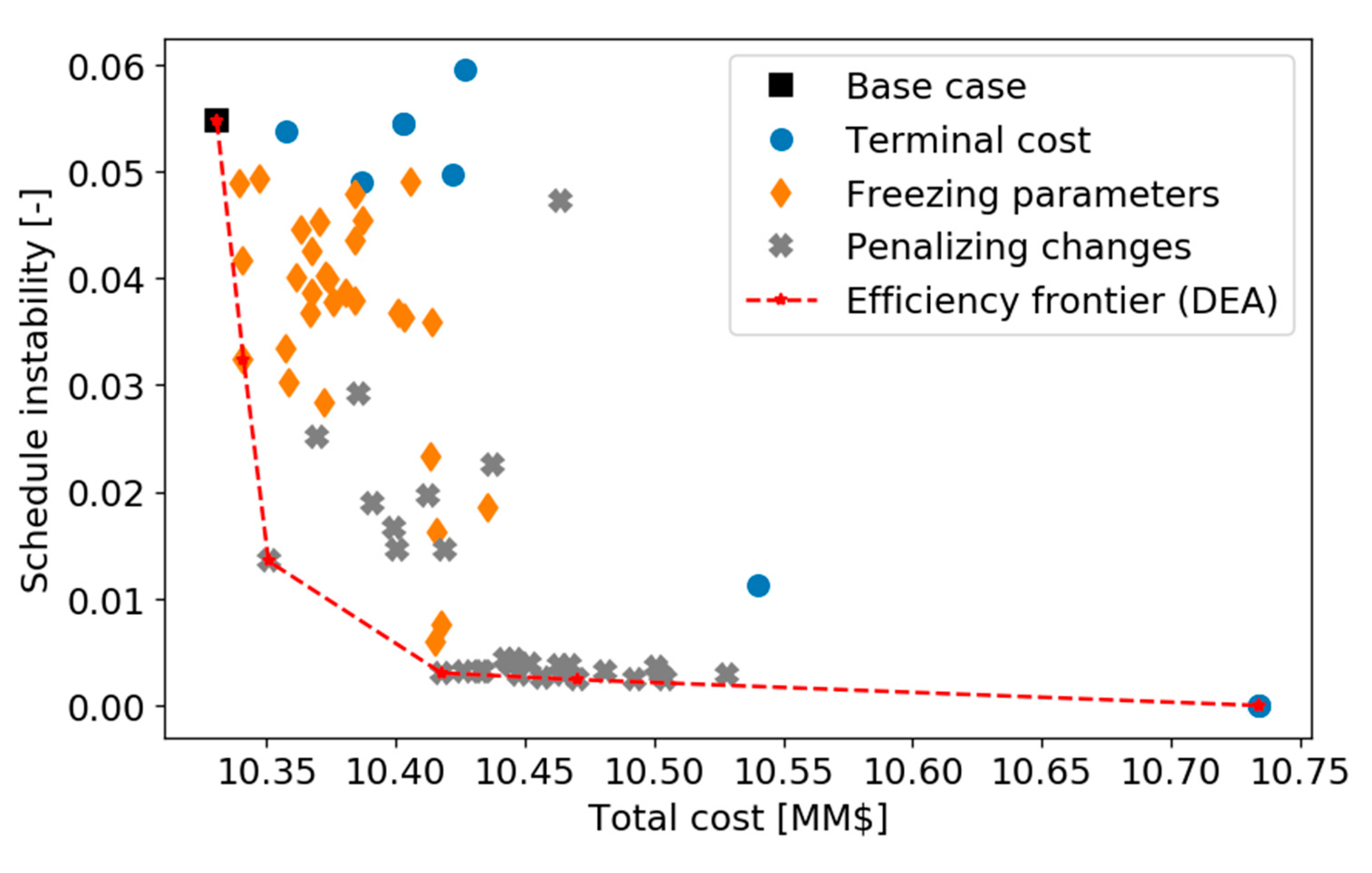
All the alternatives presented to improve closed-loop schedule stability were effective in doing so. In all scenarios considered, improving schedule stability came at the expense of the total operating cost, demonstrating a trade-off between how fast the system reacts to disturbance and the long-term predictability of the schedule. A data envelope analysis (DEA) [43,44] was used to evaluate this trade-off for all the scenarios simultaneously considered in all the alternatives. Each point in the DEA represents a solution of the closed-loop optimal scheduling problem, using any alternative to improve stability and the specifications of its parameters. Hence, there are 71 points in total—one base case, 10 for the terminal cost alternative, 30 for the freezing decisions alterative, and 30 for the penalizing schedule variability alternative. The total operating cost and the average overall weighted instability of each schedule were considered as “inputs” to the standard representation of the DEA, while there were no “outputs”, and an “efficiency” was calculated for each point by solving a linear programming problem.
The results of the DEA are presented in Figure 13, where the points are classified according to the closed-loop alternative used to improve stability, and the efficiency frontier was constructed from the DEA. The points that lay on the frontier have a 100% efficiency (i.e., represent the best combination of the inputs, and no other data point available can be as good or better) and all other points underperform with respect to those. All the points for the terminal cost alternative lay inside the frontier; thus, they are not as efficient as those defined by the other alternatives or even as the base case, which did not consider stability in the online schedule optimization. This underperformance of the terminal cost alternative is because the reference point used to ensure closed-loop stability, although stable, correspond to the worst conditions to operate the preheat train. The freezing decisions and variability penalty alternatives both improved the closed-loop schedule stability but compromised the operational cost. For these data points, two clusters are observed: one for the freezing decisions alternative that, on average, reduces the schedule instability without a large cost penalty and another for the variability penalty alternative that, on average, achieves a larger improvement in stability but with a larger increase in operating cost. Some of the data points of the two clusters overlap, representing intermediate solutions.
For this case study, the DEA suggests that the variability penalty method is the better approach to reduce schedule instability, while still achieving a good economic performance. The terminal cost alternative proved to be the least efficient, whereas freezing decisions in successive schedules increased stability, but could be too restrictive in the presence of disturbances, such that not all the economic benefits of implementing an online fouling mitigation strategy were achieved.
6. Closed-Loop Schedule Stability of an Industrial Preheat Train
This section analyzes the closed-loop performance and stability of the online optimal cleaning scheduling and control of an industrial preheat train under dynamic and variable operation.
6.1. Case Study 2—Definition
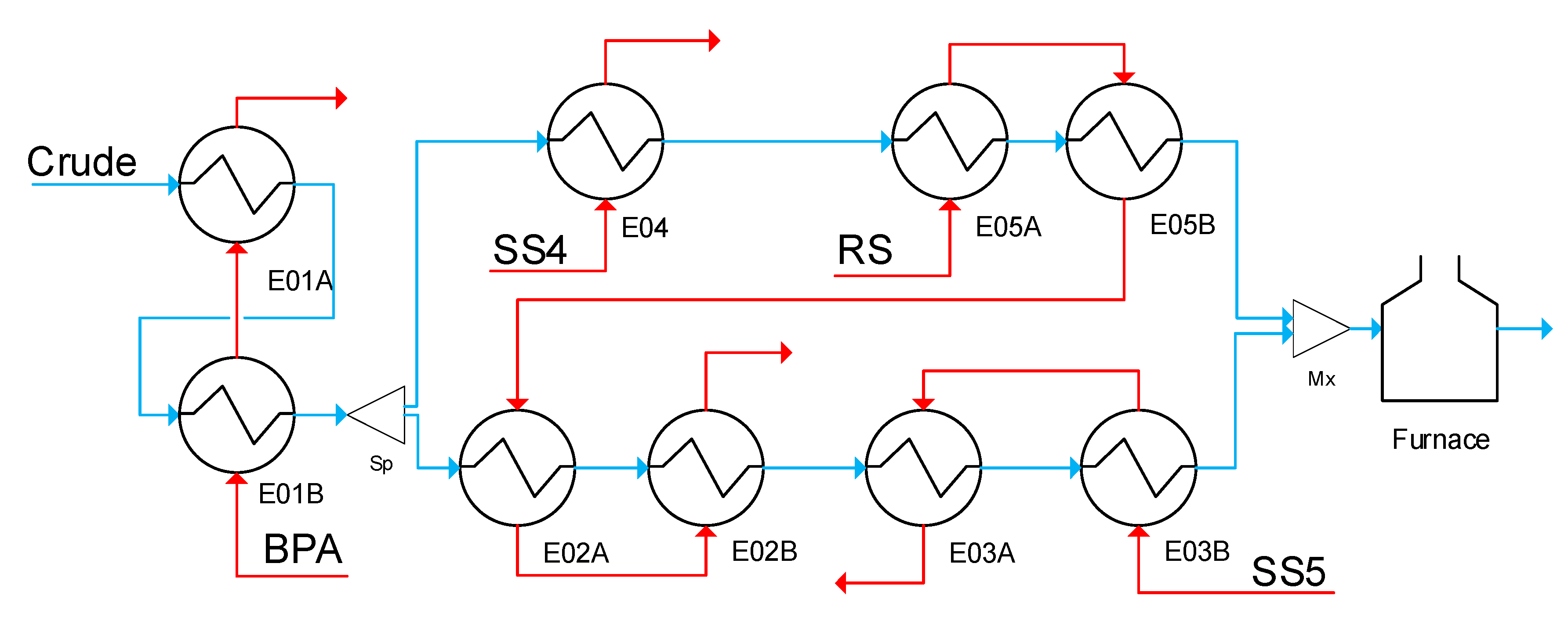
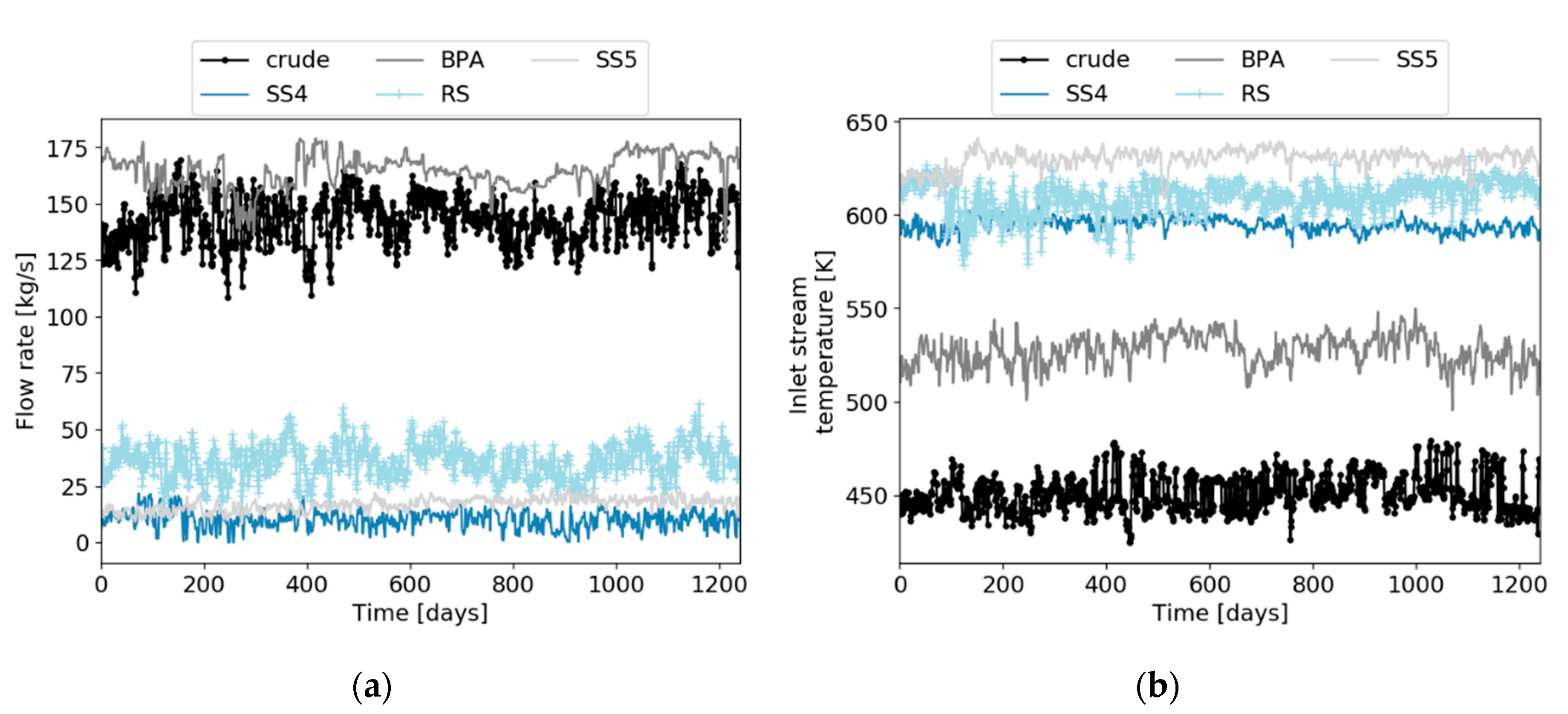
This case study involves a network with five heat exchangers, four of which are double shells (modeled as nine exchangers overall) in the hot end of a real refinery preheat train (Figure 14). It was based on the network and operating conditions presented in [45,46]. There is one control degree of freedom, as the flow split of crude oil through the parallel branches is not constrained but bound between 20% and 80%. Plant measurements of flow rates and streams temperature were available as daily averages over 1240 days. Figure 15 shows the flowrates and temperatures of the five inlet streams to the network (crude oil and five recycle streams) which were used to characterize the variability of the inlet streams. The design specifications of the heat exchangers are presented in Table A2 (Appendix A), together with fouling and aging parameters, while cost parameters used are presented in Table A3 (Appendix A). A dynamic model of this preheat train was validated against the plant data in [1] with excellent results and was used here as the “plant” model.
A controlled degree of model plant mismatch was introduced by modifying the fouling deposition constants of each exchanger in the plant model at every sampling time. This aimed to mimic the effect of processing different crudes or crude blends, as they have different fouling propensity. The deposition constants in the plant simulation changed over time, but their actual value was unknown to all predictive models used in the online optimization approach. The variability of the deposition constants in each exchanger was modeled as a pseudo random process around their average values, estimated using the actual measurements (i.e., outlet temperature of the tube side and shell side of each exchanger). Because all exchangers process the same crude at a given time, their deposition constants are not independent, and their correlation was captured when defining their variability. The average deposition constant and its variability were different for each exchanger in the network. The box plots in Figure 16 show their median and ranges for all exchangers.
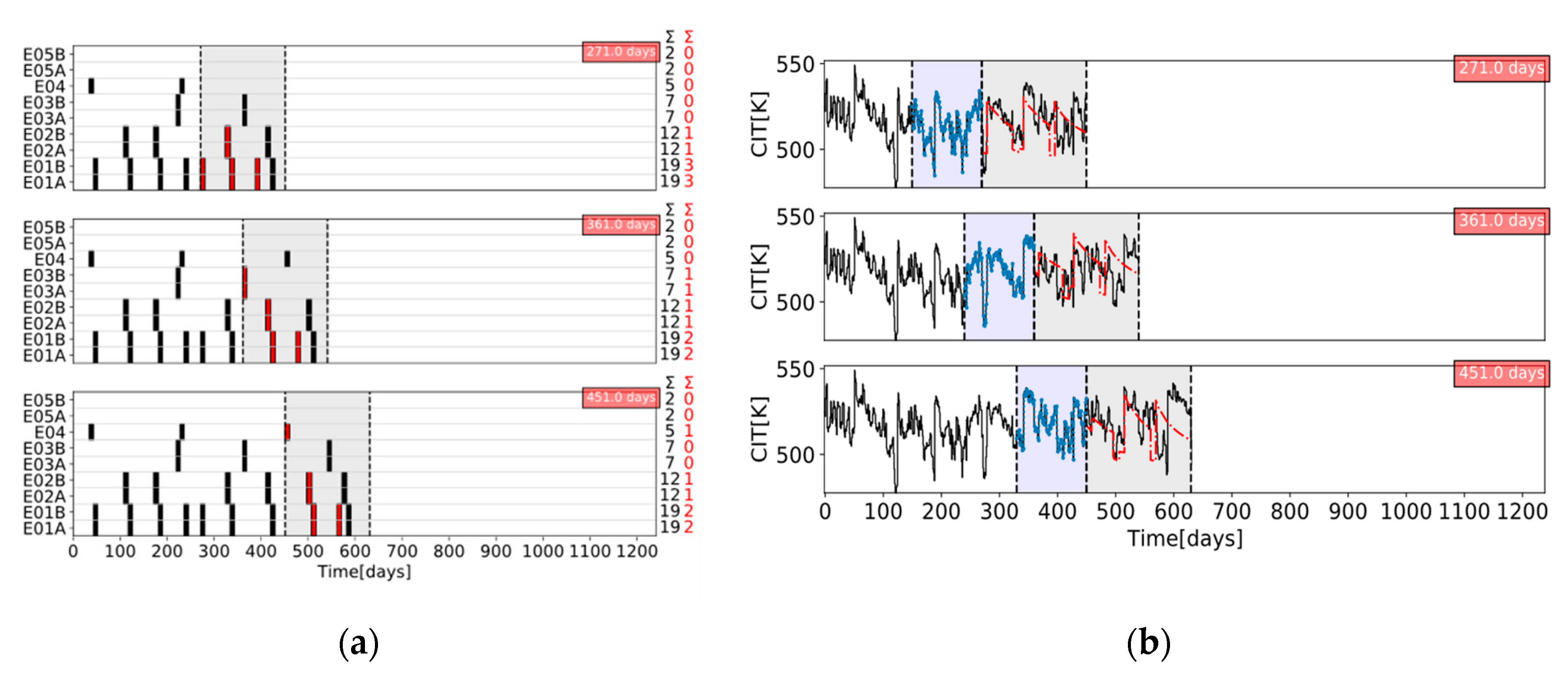
A closed-loop simultaneous optimization of the flow distribution and cleaning schedule was carried out over 1240 days, starting with all exchangers in a clean state. The economic performance optimization case, ignoring schedule stability (base case), was detailed in [1]. For this case, Figure 17 presents the cleaning schedule and a key temperature (the crude oil temperature at the entrance of the furnace, CIT), as predicted and executed at three successive sampling times.
6.2. Results and Discussion
The online optimal cleaning scheduling and flow control problem was solved using the following settings: for the feedback loops, a predictive control horizon of 10 days, an update frequency of 1 day, and a of 20 days for the control layer; for the scheduling layer, a of 120 days, an update frequency of 90 days, and of 180 days. The variability penalty alternative to penalize changes between consecutive schedules, described in Section 4.3, was used. The two penalty parameters on task allocation, , and on task timing, , were varied, defining different settings for the online optimization. Results are compared against the base case, which did not consider instability, in terms of schedule stability and total operating cost.
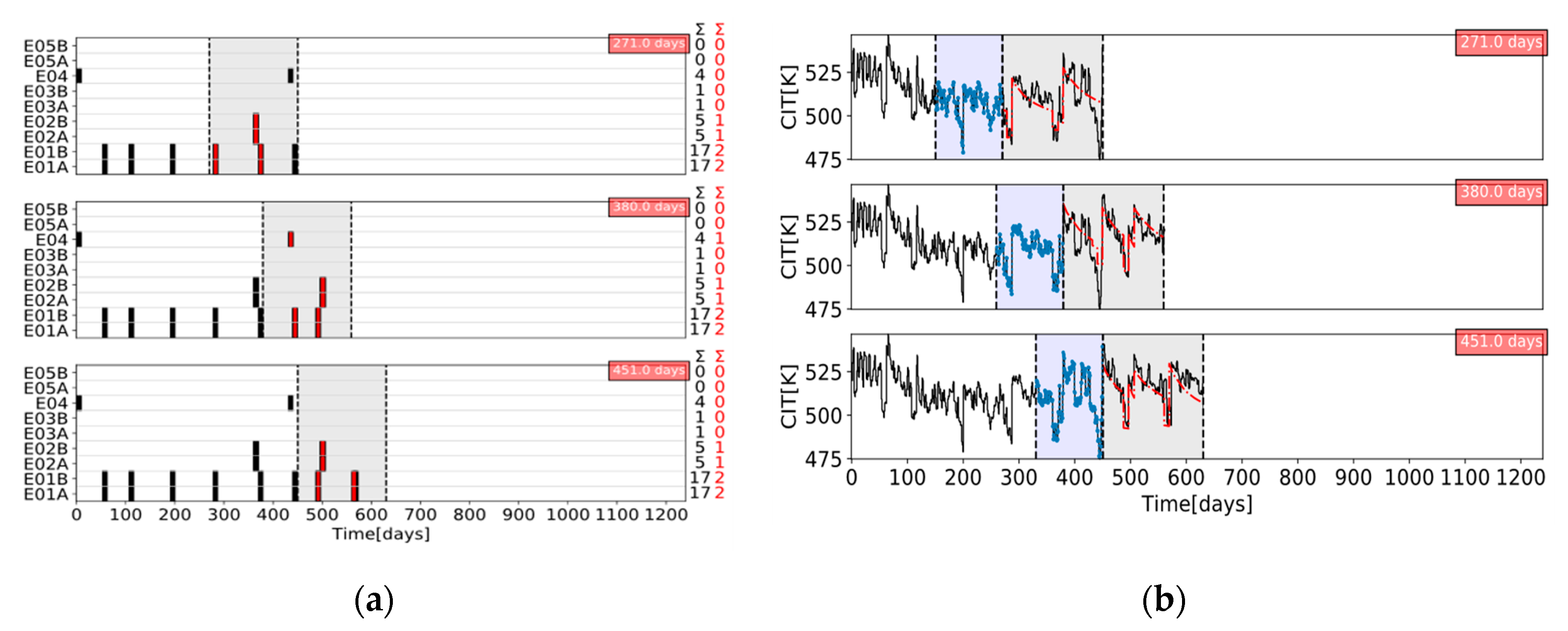
The closed-loop performance with the variability penalty formulation is presented in Figure 18 as the schedules and profiles of a key temperature (the crude oil temperature at the entrance of the furnace, CIT) at three successive schedule updates.
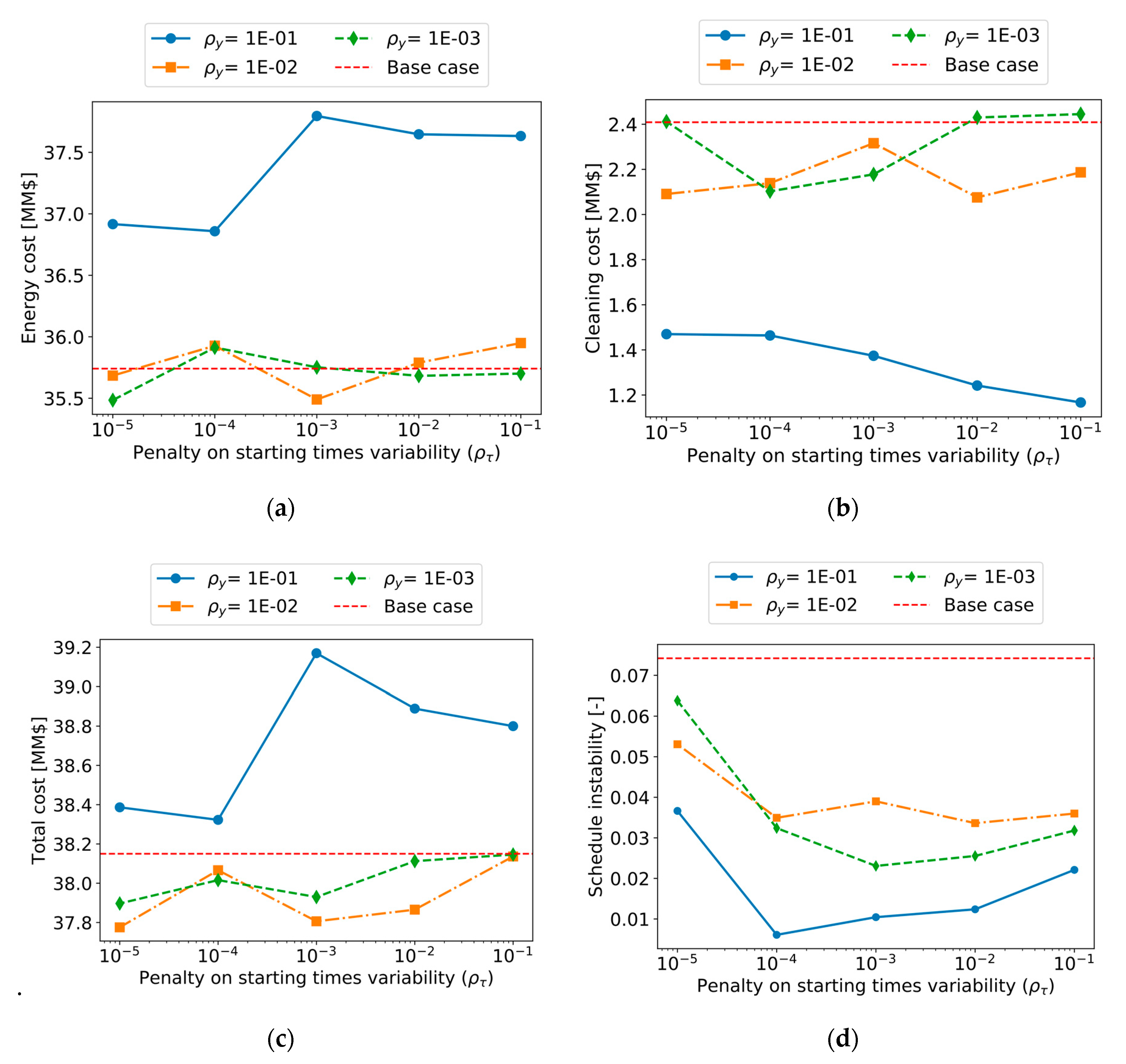
Figure 19a–c show the energy cost (a), the cleaning cost (b), and the total operating cost (c). The closed-loop average overall time-weighted instability is presented in Figure 19d (without the variability bars in the metric for clarity). The scenarios with a task allocation penalty, , of have consistently a larger operating cost, up to 1.0 million USD, than the base case. This cost increase is due to larger energy cost and fewer cleanings during the overall online operation. However, these scenarios exhibit the lowest schedule instability. Fewer cleanings are predicted at every schedule update because adding new cleanings to or removing some from a previous schedule are heavily penalized. The predicted cleaning schedules, therefore, have minimal changes between updates. This also inhibits the ability of the scheduling feedback loop to react to disturbances and introduce operational changes to mitigate fouling and minimize the cost of the operation.
With values of the task allocation penalty parameter , the closed-loop performance is not very different from the base case, and it could even improve it, reducing the total operating cost by 0.37 million USD in one case. In addition, the corresponding schedules have a lower instability than the base case, meaning that they improved both the closed-loop performance and the closed-loop stability at the same time. All scenarios with have lower cost than the base case, but larger closed-loop instability than those with . This observed simultaneous improvement in the two metrics of closed-loop performance contradicts the expectations. A possible explanation is that this case reflects a specific realization of the uncertainty, disturbances, variability in the operation, and forecasting scenarios adopted. The input flow rates and stream temperature in the plant were assumed to change constantly, while the predictive model of the scheduling layer uses at each evaluation only a constant forecast for each input, defined as a time-moving average of recent past values.
The effect of the penalty parameter on the task timing instability is not as significant as that of the penalty parameter on the task allocation instability. The operating cost increases only slightly when the task timing penalty increases from to , but this difference is no more than 0.37 million USD for while, for the operating cost ranged from 38.4 million to 39.2 million USD, depending on the task timing penalty, . For the overall closed-loop performance, the starting time of the cleanings is not as important as the allocation of cleanings to heat exchangers. Under variable and uncertain operating conditions, modifying the starting time of an already scheduled cleaning task for a given unit did not have a big potential to reduce the energy cost, but could improve schedule stability. A reduction in schedule instability was observed between and , whereas the changes in instability were minimal when increases further. The lowest penalty, , allowed the largest variability in the cleaning starting times between consecutive schedules. For larger values of the changes in the predicted cleaning time were minimal, and most of the schedule instability came from changes in the allocation of cleanings to the heat exchanger as new cleanings were predicted.
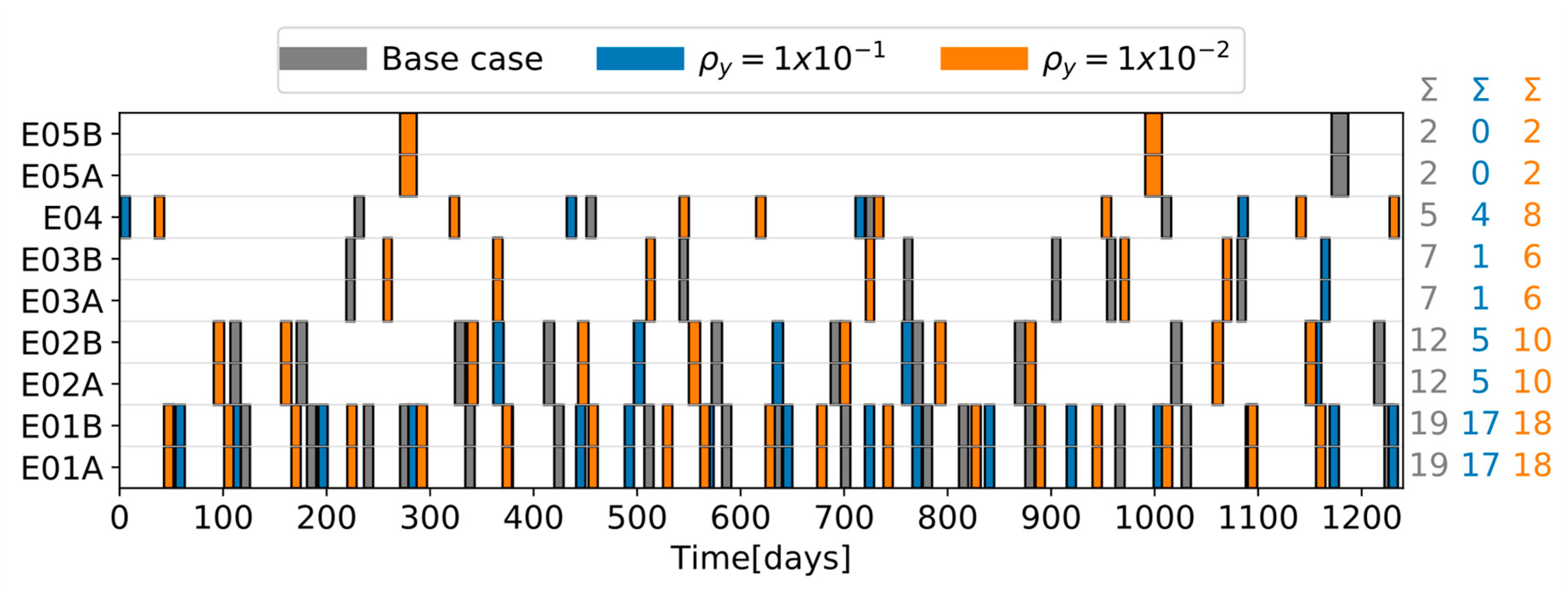
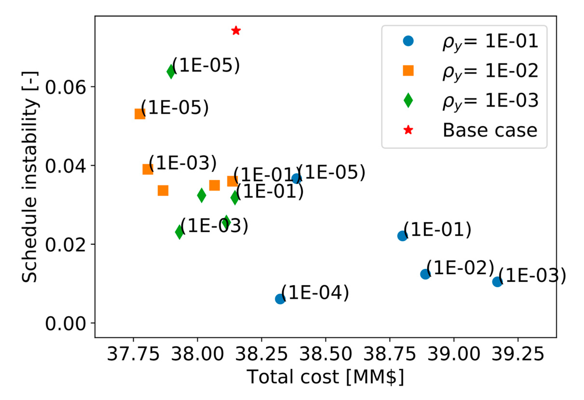
Figure 20 compares the cleaning schedule obtained (as executed by the end of the 1240 day operation) for three scenarios: (i) the base case without stability consideration, (ii) a variability penalty case that achieved better closed-loop stability while increasing the operating cost (), and (iii) a variability penalty case that improved both the closed-loop stability and the operating cost with respect to the base case (). The total number of cleanings, indicated for the exchanger in the columns on the right of Figure 20, changes significantly between the scenarios. The second scenario, with resulted in fewer cleanings and longer times between cleanings of the same exchangers, while the other two scenarios had similar cleaning schedules. Although the final closed-loop schedules of the base case (i) and scenario (iii) are similar, their generation in a receding horizon and their performance were different. In the base case (i), the calculated instability value, 0.075, results mainly from adding to a predicted schedule new cleanings that have to be immediately executed. This is not practical from a planning perspective, if the response to cleaning decisions and supply of resources needed for their execution is not immediate. In scenario (iii), such actions are penalized, thus occur less often, and most of the schedule variability can be attributed to the changes in the starting time of the predicted cleanings. A Pareto plot of all solutions explored is given in Figure 21.
In general, the penalization of schedule changes achieves more stable schedules, but reduces the ability of the system to react to changes. Due to the high variability and uncertainty of the operation (and possibly the existence of multiple local optima to the nonconvex MINLP scheduling problem), the trade-off between stability and performance is less clear.
7. Conclusions and Perspectives
The closed-loop schedule stability problem was addressed in this work with an application to the online cleaning scheduling and control of refinery preheat trains under fouling. The various metrics developed to quantify schedule instability for online scheduling account for distinct aspects, such as changes in task allocation, task sequence, starting time of the task, and the earlier or later occurrence of such changes in the future scheduling horizon. The results show that the metrics are useful to characterize the stability of successive schedules, as well as to identify sources of instability and ways to mitigate it. Further stability metric variations could be easily developed (for example, ways of assigning weights to distinct contributions to a schedule change) on the basis of the methods proposed.
It was demonstrated that such stability considerations can be practically and, in a rather general way, introduced in a closed-loop NMPC formulation of the optimal scheduling and control problem, and solved online over a moving horizon, in terms of penalties in an economic objective or via additional constraints. The result is a formulation which enables to specify both schedule stability and performance requirements, explore the balance between schedule reactivity and disturbance rejections, and establish the optimal trade-off between schedule stability and economic benefits.
The above methods were demonstrated for the online cleaning scheduling and flow control of refinery preheat trains, a challenging application with significant economic, safety, and environmental impact. An illustrative, small but realistic case study was followed by a demanding industrial case study. Results show that, of the three alternatives evaluated, the terminal cost penalty proved to be inefficient in this case. The other two (fixing some decision in the prediction horizon, and penalizing schedule changes between consecutive evaluations) showed improvements in the closed-loop schedule stability, against various degrees of economic penalties. The results highlight the importance of including stability considerations in an economically oriented online scheduling problem, as a way to obtain feasible solutions for operators over long operating horizons without sacrificing the benefits of a reactive system to reject disturbances or take advantage of them.
Nevertheless, there are still open questions related to the definition of the penalties or bounds in the schedule instability mitigation strategies, as well as the definition of acceptable ranges of schedule stability or instability. Extensions of this work include dealing with multiple task types (as already outlined in the paper) and, for longer-term development, the use of global solution methods and formally incorporating uncertainty in models and solutions.
Application of the metrics developed in this manuscript is not restricted to the specific closed-loop NMPC scheduling implementation detailed here. They are useful to assess schedule stability in general regardless of how schedules are calculated, only relying on the existence of two consecutive evaluations or predictions of the schedule with a common period. The two consecutive instances may have different control horizons, scheduling horizons, or update frequency. Lastly, although this work dealt with a specific application (the optimization of refinery heat exchanger networks subject to fouling), the formulations and solution approach demonstrated here should be applicable with small modifications to other cases where closed-loop scheduling and control of dynamic systems is important, such as batch and semi-continuous processes.
Author Contributions
Data curation, writing—original draft preparation, F.L.S.; formal analysis, investigation, software, and validation, F.L.S.; conceptualization, methodology, F.L.S. and S.M.; project administration, resources, supervision, and writing—review and editing, S.M. All authors have read and agreed to the published version of the manuscript.
Funding
One of the authors (FLS) gratefully acknowledges the receipt of a President’s Scholarship from Imperial College London in support of his PhD studies.
Conflicts of Interest
The authors declare no conflict of interest
Nomenclature
| Subscripts | Description | |
| Related to the control layer in the online optimization approach | ||
| Deposit layer | ||
| Overall schedule instability | ||
| Overall weighted schedule instability | ||
| Related to the scheduling layer in the online optimization approach | ||
| Task timing instability | ||
| Task allocation instability | ||
| Symbol | Units | Description |
| Tube inner diameter | ||
| Activation energy of fouling reaction | ||
| - | Schedule instability | |
| - | Terminal cost in the objective function of MPC | |
| Carbon emission factor (0.015) | ||
| - | Discrete points (columns) in a schedule representation | |
| - | Units (rows) in a schedule representation | |
| Pressure | ||
| Carbon price (30 USD/ton) | ||
| Cleaning cost per unit | ||
| Energy price (25 USD/MW) | ||
| - | Prandtl number | |
| Furnace duty | ||
| Universal gas constant | ||
| - | Reynolds number | |
| Thermal resistance of the deposit—fouling resistance | ||
| Time | ||
| Film temperature | ||
| Shell temperature | ||
| Tube side temperature | ||
| - | Running cost in the MPC objective function | |
| - | Decreasing sequence of weights for calculation | |
| - | Single entry of a schedule matrix | |
| - | Binary variable for cleanings (1, cleaning, 0 operating) | |
| Deposition constant | ||
| γ | m2K/JPa | Removal constant |
| Deposit thickness | ||
| Bounds on the changes of cleaning times | ||
| Thermal conductivity | ||
| - | Penalty in objective functions | |
| Shear stress | ||
| Starting time of a cleaning action | ||
| Update interval of scheduling feedback loop | ||
| - | Weights in the MHE objective function | |
| - | Heat exchanger network | |
| - | Set of heat exchangers | |
| Future prediction horizon | ||
| - | Nonlinear programming | |
| - | Nonlinear model predictive control | |
| - | Moving horizon estimator | |
| - | Model predictive control | |
| Overlapping time in the future prediction horizon | ||
| Past estimation horizon | ||
Appendix A
The model parameters and specifications for the simple case study are presented in Table A1, while those for the industrial case study are presented in Table A2. Other costs and furnace efficiency are given in Table A3.

Table A1.
Exchanger, fouling model, and cleaning specifications for the simple case study.
| HEX1 | HEX2A | HEX2B | HEX2C | |
|---|---|---|---|---|
| Shell diameter (mm) | 1295 | 1400 | 1400 | 1400 |
| Tube inner diameter (mm) | 19.86 | 19.86 | 19.86 | 19.86 |
| Tube outer diameter (mm) | 25.40 | 25.40 | 25.40 | 25.40 |
| Tube length (m) | 6100 | 5800 | 5800 | 6100 |
| Number of tubes | 800 | 600 | 600 | 600 |
| Number of passes | 2 | 2 | 2 | 4 |
| Baffle cut (%) | 25 | 25 | 25 | 25 |
| Tube layout (°) | 45 | 45 | 45 | 45 |
| Number of baffles | 8 | 6 | 6 | 7 |
| Surface roughness | 0.046 | 0.046 | 0.046 | 0.046 |
| Deposition constant (m2 K/J) | 0.0075 | 0.0085 | 0.0085 | 0.0065 |
| Removal constant (m4 K/NJ) | 4.5 × 10⁻¹² | 4.0 × 10⁻¹² | 4.0 × 10⁻¹² | 4.5 × 10⁻¹² |
| Fouling activation energy (J/mol) | 35,000 | 33,000 | 33,000 | 38,000 |
| Ageing frequency factor (1/day) | 0.00 | 0.00 | 0.00 | 0.00 |
| Ageing activation energy (J/mol) | 50,000 | 50,000 | 50,000 | 50,000 |
| Cleaning time (days) | 10 | 10 | 10 | 10 |
| Cleaning cost (USD) | 30,000 | 30,000 | 30,000 | 30,000 |
Table A2.
Exchanger, fouling model and cleaning specifications for the industrial case study.
| E01A | E01B | E02A | E02B | E03A | E03B | E04 | E05A | E05B | |
|---|---|---|---|---|---|---|---|---|---|
| Shell diameter (mm) | 1245 | 1194 | 1397 | 1397 | 990 | 990 | 1270 | 1397 | 1397 |
| Tube inner diameter (mm) | 19.86 | 19.86 | 19.86 | 19.86 | 13.51 | 13.51 | 19.86 | 19.86 | 19.86 |
| Tube outer diameter (mm) | 25.40 | 25.40 | 25.40 | 25.40 | 19.05 | 19.05 | 25.40 | 25.40 | 25.40 |
| Tube length (m) | 6090 | 6090 | 6090 | 6090 | 6090 | 6090 | 6090 | 6090 | 6090 |
| Number of tubes | 764 | 850 | 880 | 880 | 630 | 630 | 888 | 880 | 880 |
| Number of passes | 2 | 2 | 4 | 4 | 2 | 2 | 4 | 4 | 4 |
| Baffle cut (%) | 25 | 22.5 | 25 | 25 | 25 | 25 | 17 | 25 | 25 |
| Tube layout (°) | 45 | 45 | 45 | 45 | 45 | 45 | 45 | 45 | 45 |
| Number of baffles | 5 | 7 | 18 | 18 | 20 | 20 | 9 | 18 | 18 |
| Surface roughness | 0.046 | 0.046 | 0.046 | 0.046 | 0.046 | 0.046 | 0.046 | 0.046 | 0.046 |
| Deposition constant (m2 K/J) | 0.0045 | 0.0041 | 0.0036 | 0.0036 | 0.0012 | 0.0014 | 0.0032 | 0.0040 | 0.0038 |
| Removal constant (m4 K/NJ) | 1.69 × 10⁻¹¹ | 1.53 × 10⁻¹¹ | 1.28 × 10⁻¹¹ | 1.30 × 10⁻¹¹ | 3.77 × 10⁻¹¹ | 4.54 × 10⁻¹² | 1.14 × 10⁻¹¹ | 1.46 × 10⁻¹¹ | 1.39 × 10⁻¹¹ |
| Fouling activation energy (J/mol) | 28,500 | 28,500 | 28,500 | 28,500 | 28,500 | 28,500 | 28,380 | 28,500 | 28,500 |
| Ageing frequency factor (1/day) | 0.00 | 0.00 | 0.00 | 0.00 | 0.00 | 0.00 | 0.00 | 0.00 | 0.00 |
| Ageing activation energy (J/mol) | 50,000 | 50,000 | 50,000 | 50,000 | 50,000 | 50,000 | 50,000 | 50,000 | 50,000 |
| Cleaning time (days) | 9 | 9 | 10 | 10 | 8 | 8 | 9 | 16 | 16 |
| Cleaning cost (USD) | 27,000 | 27,000 | 30,000 | 30,000 | 24,000 | 24,000 | 27,000 | 48,000 | 48,000 |
Table A3.
Costs and furnace specifications.
| Fuel cost (USD/MWh) | 27 |
| Production cost (USD/kg) | 0.23 |
| Carbon cost (USD/t) | 30 |
| Carbon emission factor (t CO2/MWh) | 0.015 |
| Furnace efficiency (%) | 90 |
References
- Santamaria, F.L.; Macchietto, S. Online Integration of Optimal Cleaning Scheduling and Control of Heat Exchanger Networks under Fouling. Ind. Eng. Chem. Res. 2019, 59, 2471–2490. [Google Scholar] [CrossRef]
- Bajestani, M.A.; Banjevic, D.; Beck, J.C. Integrated maintenance planning and production scheduling with Markovian deteriorating machine conditions. Int. J. Prod. Res. 2014, 52, 7377–7400. [Google Scholar] [CrossRef]
- Li, R.; Ma, H. Integrating Preventive Maintenance Planning and Production Scheduling under Reentrant Job Shop. Math. Probl. Eng. 2017, 2017, 1–9. [Google Scholar] [CrossRef]
- Kopanos, G.M.; Puigjaner, L. Integrated operational and maintenance planning of production and utlity systems. In Solving Large-Scale Production Scheduling and Planning in The Process Industries; Springer: London, UK, 2019. [Google Scholar]
- Vieira, G.E.; Herrmann, J.W.; Lin, E. Rescheduling Manufacturing Systems: A Framework of Strategies, Policies, and Methods. J. Sched. 2003, 6, 39–62. [Google Scholar] [CrossRef]
- Chu, Y.; You, F. Integration of scheduling and control with online closed-loop implementation: Fast computational strategy and large-scale global optimization algorithm. Comput. Chem. Eng. 2012, 47, 248–268. [Google Scholar] [CrossRef]
- Suwa, H.; Sandoh, H. Online Scheduling in Manufacturing; Springer: London, UK, 2013. [Google Scholar]
- Kopanos, G.M.; Capón-García, E.; Espuña, A.; Puigjaner, L. Costs for Rescheduling Actions: A Critical Issue for Reducing the Gap between Scheduling Theory and Practice. Ind. Eng. Chem. Res. 2008, 47, 8785–8795. [Google Scholar] [CrossRef]
- Méndez, C.A.; Cerdá, J.; Grossmann, I.E.; Harjunkoski, I.; Fahl, M. State-of-the-art review of optimization methods for short-term scheduling of batch processes. Comput. Chem. Eng. 2006, 30, 913–946. [Google Scholar] [CrossRef] [Green Version]
- Gupta, D.; Maravelias, C.T. On deterministic online scheduling: Major considerations, paradoxes and remedies. Comput. Chem. Eng. 2016, 94, 312–330. [Google Scholar] [CrossRef] [Green Version]
- Gupta, D.; Maravelias, C.T.; Wassick, J.M. From rescheduling to online scheduling. Chem. Eng. Res. Des. 2016, 116, 83–97. [Google Scholar] [CrossRef]
- Panchal, C.B.; Huangfu, E.-P. Effects of Mitigating Fouling on the Energy Efficiency of Crude-Oil Distillation. Heat Transf. Eng. 2000, 21, 3–9. [Google Scholar] [CrossRef]
- Diaby, A.L.; Luong, L.; Yousef, A.; Addai-Mensah, J. A Review of Optimal Scheduling Cleaning of Refinery Crude Preheat Trains Subject to Fouling and Ageing. Appl. Mech. Mater. 2012, 148, 643–651. [Google Scholar] [CrossRef]
- Nategh, M.; Malayeri, M.R.; Mahdiyar, H. A Review on Crude Oil Fouling and Mitigation Methods in Pre-Heat Trains of Iranian Oil Refineries. J. Oil Gas Petrochem. Technol. 2017, 4, 1–17. [Google Scholar]
- Coletti, F.; Hewitt, G.F. Crude Oil Fouling. Deposit Characterization, Measurements, and Modelling, 1st ed.; Gulf Professional Publishing: London, UK, 2015. [Google Scholar]
- Santamaria, F.L.; Macchietto, S. Integration of Optimal Cleaning Scheduling and Control of Heat Exchanger Networks Undergoing Fouling: Model and Formulation. Ind. Eng. Chem. Res. 2018, 57, 12842–12860. [Google Scholar] [CrossRef]
- Tian, J.; Wang, Y.; Feng, X. Simultaneous optimization of flow velocity and cleaning schedule for mitigating fouling in refinery heat exchanger networks. Energy 2016, 109, 1118–1129. [Google Scholar] [CrossRef]
- Cott, B.; Macchietto, S. Minimizing the effects of batch process variability using online schedule modification. Comput. Chem. Eng. 1989, 13, 105–113. [Google Scholar] [CrossRef]
- Méndez, C.A.; Cerda, J. Dynamic scheduling in multiproduct batch plants. Comput. Chem. Eng. 2003, 27, 1247–1259. [Google Scholar] [CrossRef]
- Novas, J.M.; Henning, G.P. Reactive scheduling framework based on domain knowledge and constraint programming. Comput. Chem. Eng. 2010, 34, 2129–2148. [Google Scholar] [CrossRef]
- Vin, J.P.; Ierapetritou, M.G. A New Approach for Efficient Rescheduling of Multiproduct Batch Plants. Ind. Eng. Chem. Res. 2000, 39, 4228–4238. [Google Scholar] [CrossRef]
- Ave, G.D.; Alici, M.; Harjunkoski, I.; Engell, S. An Explicit Online Resource-Task Network Scheduling Formulation to Avoid Scheduling Nervousness. Comput. Aided Chem. Eng. 2019, 46, 61–66. [Google Scholar]
- Macchietto, S. Integrated Batch Processing: A model for advanced manufacturing. In Proceedings of the APACT Conference Advances in Process Analytics and Control Technology, Birmingham, UK, 20–22 April 2005. [Google Scholar]
- Macchietto, S. Engineering success: What does it take to get PSE technologies used? In Computer Aided Chemical Engineering; Kiss, A.A., Zondervan, E., Lakerveld, R., Özkan, L., Eds.; Elsevier: Amsterdam, The Netherlands, 2019; Volume 46, Part A, pp. 85–90. [Google Scholar]
- Rodrigues, M.T.M.; Gimeno, L.; Passos, C.A.S.; Campos, M.D. Reactive scheduling approach for multipurpose chemical batch plants. Comput. Chem. Eng. 1996, 20, S1215–S1220. [Google Scholar] [CrossRef]
- Ferrer-Nadal, S.; Méndez, C.A.; Graells, M.; Puigjaner, L. Optimal Reactive Scheduling of Manufacturing Plants with Flexible Batch Recipes. Ind. Eng. Chem. Res. 2007, 46, 6273–6283. [Google Scholar] [CrossRef]
- Subramanian, K.; Rawlings, J.B.; Maravelias, C.T. Economic model predictive control for inventory management in supply chains. Comput. Chem. Eng. 2014, 64, 71–80. [Google Scholar] [CrossRef]
- Hewitt, G.F.; Shires, G.L.; Bott, T.R. Process Heat Transfer; CRC Press: Boca Raton, FL, USA, 1994. [Google Scholar]
- Thulukkanam, K. Shell and tube heat exchanger design. In Heat Exchanger Design Handbook; CRC Press: Boca Raton, FL, USA, 2013; pp. 237–336. [Google Scholar]
- Ebert, W.; Panchal, C.B. Analysis of Exxon Crude-Oil-Slip Stream Coking Data; Argonne National Lab: Lemont, IL, USA, 1995; retrieved from University of North Texas Digital Library.
- Santamaría, F.L.; Macchietto, S. Model validation for the optimization of refinery preheat trains under fouling. In Proceedings of the Heat Exchanger Fouling and Cleaning XIII, Warsaw, Poland, 2–7 June 2019; Zettler, H.U., Ed.; Available online: http://www.heatexchanger-fouling.com/proceedings19.htm (accessed on 1 January 2020).
- Santamaria, F.L.; Macchietto, S. Integration of optimal cleaning scheduling and control of heat exchanger networks under fouling: MPCC solution. Comput. Chem. Eng. 2019, 126, 128–146. [Google Scholar] [CrossRef]
- Sridharan, S.V.; Berry, W.L.; Udayabhanu, V. Measuring Master Production Schedule Stability Under Rolling Planning Horizons. Decis. Sci. 1988, 19, 147–166. [Google Scholar] [CrossRef]
- Pujawan, I.N. Schedule nervousness in a manufacturing system: A case study. Prod. Plan. Control 2004, 15, 515–524. [Google Scholar] [CrossRef]
- Van Donselaar, K.; van den Nieuwenhof, J.; Visschers, J. The impact of material coordination concepts on planning stability in supply chains. Int. J. Prod. Econ. 2000, 68, 169–176. [Google Scholar] [CrossRef]
- Kadipasaoglu, S.N.; Sridharan, S.V. Measurement of instability in multi-level MRP systems. Int. J. Prod. Res. 1997, 35, 713–737. [Google Scholar] [CrossRef]
- Maciejowski, J.M. Predictive Control with Constraints; Prentice Hall: Upper Saddle River, NJ, USA, 2002. [Google Scholar]
- Risbeck, M.J.; Maravelias, C.T.; Rawlings, J.B. Unification of closed-loop scheduling and control: State-space formulations, terminal constraints, and nominal theoretical properties. Comput. Chem. Eng. 2019, 129, 106496. [Google Scholar] [CrossRef]
- Blackburn, J.D.; Kropp, D.H.; Millen, R.A. A Comparison of Strategies to Dampen Nervousness in MRP Systems. Manag. Sci. 1986, 32, 413–429. [Google Scholar] [CrossRef]
- Jacobs, F.; Berry, W.; Whybark, D.; Vollmann, T. Advanced MRP. In Manufacturing Planning and Control for Supply Chain Management; McGraw-Hill: New York, NY, USA, 2005. [Google Scholar]
- Coletti, F.; Macchietto, S. Refinery Pre-Heat Train Network Simulation Undergoing Fouling: Assessment of Energy Efficiency and Carbon Emissions. Heat Transf. Eng. 2011, 32, 228–236. [Google Scholar] [CrossRef]
- Macchietto, S.; Macchietto, S. A Dynamic, Distributed Model of Shell-and-Tube Heat Exchangers Undergoing Crude Oil Fouling. Ind. Eng. Chem. Res. 2011, 50, 4515–4533. [Google Scholar] [CrossRef]
- Farrell, M.J. The Measurement of Productive Efficiency. J. R. Stat. Soc. Ser. A 1957, 120, 253. [Google Scholar] [CrossRef]
- Charnes, A.; Cooper, W.W.; Rhodes, E. Measuring the efficiency of decision making units. Eur. J. Oper. Res. 1978, 2, 429–444. [Google Scholar] [CrossRef]
- Coletti, F. Multi-Scale Modelling of Refinery Pre-Heat Trains Undergoing Fouling for Improved Energy Efficiency; Imperial College of London: London, UK, 2010. [Google Scholar]
- Lanchas-Fuentes, L.; Diaz-Bejarano, E.; Coletti, F.; Macchietto, S. Management of cleaning types and schedules in refinery heat exchangers. In Proceedings of the 12th International Conference on Heat Transfer, Fluid Mechanics and Thermodynamics HEFAT2016, Costa de Sol, Spain, 11–13 July 2016. [Google Scholar]
Figure 1.
Top left: 14 day schedule of beer production (140 process units, 26 recipe families). Top right: 5 day production schedule of chilled desserts for northern Europe (35 product families, daily changes) as of 4:00 a.m. on a Saturday morning. Bottom: Online rescheduling every minute; the red vertical line separates the historical schedule (as actually happened) from the predicted one (adapted from [23]).

Figure 2.
Simplified representation of the online, integrated optimal cleaning scheduling and control of preheat trains subject to fouling and disturbances.
Figure 2.
Simplified representation of the online, integrated optimal cleaning scheduling and control of preheat trains subject to fouling and disturbances.

Figure 3.
Representation of sources of scheduling instability and the elements used to quantify it.

Figure 4.
Schedule matrix representation of a schedule for a simple example with a unique task and the overlapping interval discretized in 8 intervals. (a) Schedule updated at time ; (b) schedule updated at time .
Figure 4.
Schedule matrix representation of a schedule for a simple example with a unique task and the overlapping interval discretized in 8 intervals. (a) Schedule updated at time ; (b) schedule updated at time .

Figure 5.
Schematic representation of freezing some scheduling decisions for improving closed-loop schedule instability.
Figure 5.
Schematic representation of freezing some scheduling decisions for improving closed-loop schedule instability.

Figure 6.
Preheat train structure of the simple case study.

Figure 7.
Case study 1, base case—predicted (red) fouling resistance in HEX2B at 91 and 106 days. Black lines show the fouling resistance observed in the final record. Vertical lines correspond to cleanings, and their shifts in time are sources of instability.
Figure 7.
Case study 1, base case—predicted (red) fouling resistance in HEX2B at 91 and 106 days. Black lines show the fouling resistance observed in the final record. Vertical lines correspond to cleanings, and their shifts in time are sources of instability.

Figure 8.
Case study 1, base case—evolution of the cleaning schedule as predicted (red) and executed (black) at various sampling times (marked in the upper right corner): (a) from 65 to 136 days; (b) from 181 to 256 days.
Figure 8.
Case study 1, base case—evolution of the cleaning schedule as predicted (red) and executed (black) at various sampling times (marked in the upper right corner): (a) from 65 to 136 days; (b) from 181 to 256 days.

Figure 9.
Case study 1, base case—evolution of closed-loop scheduling instability metrics.

Figure 10.
Case study 1—effect of the terminal cost penalty () on the closed-loop performance: (a) process economics, as total cost (left axis) and cleaning cost (right axis); (b) average schedule instability metrics and their standard deviation.
Figure 10.
Case study 1—effect of the terminal cost penalty () on the closed-loop performance: (a) process economics, as total cost (left axis) and cleaning cost (right axis); (b) average schedule instability metrics and their standard deviation.

Figure 11.
Case study 1—effect of the number of frozen periods () and the maximum allowed variation in the cleaning starting time ( ) on the closed-loop performance: (a) total operating cost; (b) average schedule overall weighted instability.
Figure 11.
Case study 1—effect of the number of frozen periods () and the maximum allowed variation in the cleaning starting time ( ) on the closed-loop performance: (a) total operating cost; (b) average schedule overall weighted instability.

Figure 12.
Case study 1—effect of the penalty on task variability () and the penalty on cleaning starting time () on the closed-loop performance: (a) total operating cost; (b) average overall weighted instability.
Figure 12.
Case study 1—effect of the penalty on task variability () and the penalty on cleaning starting time () on the closed-loop performance: (a) total operating cost; (b) average overall weighted instability.

Figure 13.
Case study 1—data envelope analysis (DEA) for all the closed-loop solutions of the scheduling and control problem.
Figure 13.
Case study 1—data envelope analysis (DEA) for all the closed-loop solutions of the scheduling and control problem.

Figure 14.
Industrial case study 2—preheat train structure.

Figure 15.
Industrial case study 2—actual measurements of the inlet stream flow rates (a) and temperature (b).
Figure 15.
Industrial case study 2—actual measurements of the inlet stream flow rates (a) and temperature (b).

Figure 16.
Industrial case study 2—box plot representing the variability in the deposition constant for each exchanger in the preheat train.
Figure 16.
Industrial case study 2—box plot representing the variability in the deposition constant for each exchanger in the preheat train.

Figure 17.
Industrial case study 2—base case online optimization (no instability reduction). (a) Cleaning schedule as predicted in three successive updates (red), and executed (black); (b) crude oil temperature at the exit of the last exchanger/inlet to furnace (CIT) as estimated (blue), predicted (red), and eventually observed (black), in three successive updates.

Figure 18.
Industrial case study 2—online optimization: variability penalty with and . (a) Cleaning schedule as predicted in three successive updates (red) and executed (black); (b) crude oil temperature at the exit of the last exchanger/inlet to furnace (CIT) as estimated (blue), predicted (red), and eventually observed (black), in three successive updates.

Figure 19.
Industrial case study 2—closed-loop performance for different penalty parameters of schedule variability: (a) energy cost; (b) cleaning cost; (c) total cost; (d) average overall time-weighted instability.
Figure 19.
Industrial case study 2—closed-loop performance for different penalty parameters of schedule variability: (a) energy cost; (b) cleaning cost; (c) total cost; (d) average overall time-weighted instability.

Figure 20.
Industrial case study 2—final cleaning schedules as executed online for the base case (no schedule instability mitigation) and two schedule instability mitigation (variability penalty with penalty parameters ). The columns on the right give the total number of cleanings of each exchanger in each case.

Figure 21.
Industrial case study 2—Pareto plot of schedule stability vs. performance, for various penalty parameters (with the value of indicated in parenthesis).
Figure 21.
Industrial case study 2—Pareto plot of schedule stability vs. performance, for various penalty parameters (with the value of indicated in parenthesis).

Table 1.
Summary of the characteristics of each feedback loop for the online optimization of the cleaning scheduling and flow control. NMPC, nonlinear model predictive control; MHE, moving horizon estimator.
Table 1.
Summary of the characteristics of each feedback loop for the online optimization of the cleaning scheduling and flow control. NMPC, nonlinear model predictive control; MHE, moving horizon estimator.
| Control Layer (C) | Scheduling Layer (S) | |||
|---|---|---|---|---|
| NMPCC | MHEC | NMPCS | MHES | |
| Minimization of operating cost | Minimization of error between data and model | Minimization of operating and maintenance cost | Minimization of error between data and model | |
| Objective function | Equation (4) | Equation (3) | Equation (5) | Equation (3) |
| Decision variables | Flow rate profiles | Fouling parameters of each exchanger | Flow rate profiles | Fouling parameters of each exchanger |
| Allocation of cleanings to exchangers | ||||
| Starting time of the cleanings | ||||
| Inputs (parameters) | Cleaning schedule | Past actions | Operating conditions | Past actions |
| Operating conditions | Past measurements | Model parameters | Past measurements | |
| Model parameters | ||||
| Time discretization | Discrete time | Discrete time | Continuous time + orthogonal collocation | Discrete time |
| Type of problem | NLP | NLP | MINLP | NLP |
| Sampling interval | From hours to days | From hours to days | From weeks to months | From weeks to months |
| Future prediction horizon (FPH) | From days to weeks | - | From months to years | - |
| Past estimation horizon (PEH) | - | From days to weeks | - | From months to years |
| Disturbances | Forecast as constant current value | Explicit (past) | Forecast as moving average of past month | Explicit (past) |
| Complicating aspects | Nonlinearities of the model | Nonlinearities of the model | Nonlinearities of the model | Nonlinearities of the model |
| Large data set in the PEH | Number of binary variables | Large data set in the PEH | ||
| Interaction of control and scheduling decisions | ||||
Publisher’s Note: MDPI stays neutral with regard to jurisdictional claims in published maps and institutional affiliations. |
© 2020 by the authors. Licensee MDPI, Basel, Switzerland. This article is an open access article distributed under the terms and conditions of the Creative Commons Attribution (CC BY) license (http://creativecommons.org/licenses/by/4.0/).
Share and Cite
MDPI and ACS Style
Lozano Santamaria, F.; Macchietto, S. Stability of Optimal Closed-Loop Cleaning Scheduling and Control with Application to Heat Exchanger Networks under Fouling. Processes 2020, 8, 1623. https://0-doi-org.brum.beds.ac.uk/10.3390/pr8121623
AMA Style
Lozano Santamaria F, Macchietto S. Stability of Optimal Closed-Loop Cleaning Scheduling and Control with Application to Heat Exchanger Networks under Fouling. Processes. 2020; 8(12):1623. https://0-doi-org.brum.beds.ac.uk/10.3390/pr8121623
Chicago/Turabian StyleLozano Santamaria, Federico, and Sandro Macchietto. 2020. "Stability of Optimal Closed-Loop Cleaning Scheduling and Control with Application to Heat Exchanger Networks under Fouling" Processes 8, no. 12: 1623. https://0-doi-org.brum.beds.ac.uk/10.3390/pr8121623
Note that from the first issue of 2016, this journal uses article numbers instead of page numbers. See further details here.