Article

Integration and Evaluation of Intra-Logistics Processes in Flexible Production Systems Based on OEE Metrics, with the Use of Computer Modelling and Simulation of AGVs

Department of Engineering Processes Automation and Integrated Manufacturing Systems, Silesian University of Technology, Konarskiego 18A, 44-100 Gliwice, Poland
*
Author to whom correspondence should be addressed.
Submission received: 13 November 2020 / Revised: 7 December 2020 / Accepted: 9 December 2020 / Published: 14 December 2020

Abstract

:
The article presents the problems connected with the performance evaluation of a flexible production system in the context of designing and integrating production and logistics subsystems. The goal of the performed analysis was to determine the parameters that have the most significant influence on the productivity of the whole system. The possibilities of using automated machine tools, automatic transport vehicles, as well as automated storage systems were pointed out. Moreover, the exemplary models are described, and the framework of simulation research related to the conceptual design of new production systems are indicated. In order to evaluate the system’s productivity, the use of Overall Equipment Efficiency (OEE) metrics was proposed, which is typically used for stationary resources such as machines. This paper aims to prove the hypothesis that the OEE metric can also be used for transport facilities such as Automated Guided Vehicles (AGVs). The developed models include the parameters regarding availability and failure of AGVs as well as production efficiency and quality, which allows the more accurate mapping of manufacturing processes. As the result, the Overall Factory Efficiency (OFE) and Overall Transport Efficiency (OTE) metrics were obtained. The obtained outcomes can be directly related to similar production systems that belong to World Class Manufacturing (WCM) or World Class Logistics (WCL), leading to the in-depth planning of such systems and their further improvement in the context of the Industry 4.0.

Graphical Abstract

1. Introduction

One of the key factors, which determine the level of competitiveness of manufacturing plants, is the ability to achieve flexible production and delivery of goods in accordance with customer requirements. Therefore, logistics and Supply Chain Management play an important role in market competition [1]. Logistic operations are carried out in two areas, internal and external to the organization. Therefore, the term “Intra-logistics” describes the organisation and realisation of internal material flow and logistic technologies as well as the goods transhipment in the industry, using technical components, partial and full systems and services [2].
In connection with the flexible production, there are also increased requirements regarding the flexibility and reliability of internal transport systems, associated with the production of short series of various products and thus requiring more transport operations [3]. In response to these needs, the Automated Guided Vehicles (AGVs) are used a lot more widely, which enables full automation of transport operations and can handle various transport routes using only computer navigation systems [4,5,6].
In order to evaluate the system’s productivity, the use of Overall Equipment Efficiency (OEE) metrics has been proposed that is usually used for stationary resources, like machines. The aim of the paper was to prove the hypothesis that the OEE metric can also be used for transport facilities such as AGVs, and there is a dependence between machine and transport effectiveness.
To investigate the influence of the intra-logistic system over the performance of the manufacturing system we have developed a conceptual model of Flexible Manufacturing System (FMS) with an automated transport system with AGVs. The model of the FMS was built with the use of FlexSim software and the OEE metric was used for system integration and description of the availability, reliability and performance parameters for machines and vehicles. Then the Discrete Event Simulation (DES) method was used for performing the series of experiments and an analysis of results is presented in form of Overall Factory Efficiency (OFE) and Overall Transport Efficiency (OTE). Our previous works [7,8,9] show that the computer simulation of the detailed model of the production line with machines, operators and robots with reliability parameters allows better representation and understanding of a real production process which is important for early design and enables front-end planning.
The AGV parameters play an important role for FMS performance; therefore, literature review about FMS, AGV and logistics issues, are presented in the next section. The subsequent sections of the paper include description of the problem, modelling and simulation experiments, results analysis and discussion and final conclusions.

2. State-of-the-Art

Many researchers in logistics have examined the influence of high-performance logistics practices on organizational performance [1,10,11]. In an attempt to drive performance improvements, managers often struggle with multiple, seemingly conflicting, objectives [1]. Logistics management is faced with a tough choice: either strive for efficiency; or strive for effectiveness. Some recent logistics research has suggested that these two performance objectives are mutually exclusive [12]. Performance measures are essential for effective management of any organization. Performance measurement provides a needed assessment of service and cost aspects of logistics execution in the supply chain. Specifically, there is little guidance regarding where a specific measure should be used and, more pointedly, where the use of the measure would be less appropriate.
Fugate et al. [13], have presented the model of logistics performance with the concept of simultaneous pursuit of efficiency, effectiveness and differentiation. However, most companies’ priorities change over time due to market and competitive dynamics. In light of this business reality, enterprises and managers must be able to identify and select new or different measures consistent with evolving organizational priorities [14].
Muthiah and Huang [15] reviewed and categorized various productivity improvement methods and productivity metrics. For example, Overall Equipment Efficiency (OEE is an established technique in World Class Manufacturing (WCM). It is used as a key performance indicator (KPI) in conjunction with lean manufacturing efforts to provide a quantifiable measurement of success. There are a few examples of the performance evaluation of manufacturing systems with the use of the OEE metric, including [16,17], but without considering the efficiency of the transport subsystem.
Muñoz-Villamizar et al. [18], have used OEE to evaluate the effectiveness of urban freight transportation systems and a framework for Overall Transport Efficiency (OTE) based on OEE factors was proposed by Dalmolen et al. [19]. McCalion [20] ask the question: is OEE relevant to logistics management and Automated Guided Vehicle (AGV) operations?
Hayes [21] suggests that the OEE can be used for eliminating the ripple effect caused by stopped vehicles and along with Six Sigma [22] can be used as a measure for World Class Logistic (WCL).
Comparing WCL with WCM, they have a lot in common. The common area is related to intra-logistic in manufacturing systems. Intra-logistic performance has a great influence over the manufacturing performance, because of inter-operational breaks which have a great impact on materials flow in flexible manufacturing system [23].
The literature review only shows a few publications on the design methodology of AGV systems and most of the them use simple KPIs as metrics [24,25,26,27,28,29]. At the time of preparing this paper, no publication was found concerning the detailed assessment of the impact of the AGVs system on the manufacturing process effectiveness that includes the OEE metric. Therefore, the studies have been undertaken in order to elaborate this problem in terms of transport and production effectiveness and to strengthen the logistics potential of the organization.

2.1. Issues Related to FMS and AGV

The flexible manufacturing system (FMS) is a fully automated production system that interconnects machines and workstations with the logistics equipment, where the entire manufacturing process is coordinated by the digital control systems such as Computer Numerical Control (CNC) or Programmable Logic Controller (PLC). Such flexible, automated manufacturing systems are intended for tasks of large typological diversity, high complexity, ensuring on-time delivery and minimal manufacturing costs, while production is unpredictable, being organized in small batches, with frequent changes [30].
The FMS has been studied over the last couple of decades and the researchers have found a variety of problems, which can be distributed in three major categories: workshop design, transportation network design and scheduling problems [31,32]. Different methods were used to solve them, including mathematical (linear, constraints, stochastic) programming, combinatorial optimization, Petri nets and scenario analysis, but computer simulation, especially Discrete Event Simulation (DES), is the most universal and widely used one [33], e.g., for the design of manufacturing systems [27], efficiency [9] and stability analysis [34] of production systems and the design of warehouse transportation systems with Automated Guided Vehicles (AGVs) [35,36,37].
The AGVs are classified as service robots for professional purposes in manufacturing environments and broad review of AGV is presented in [6,28].
Modern AGV vehicles are characterized by precision of operation, speed of movement and high reliability. They can have various equipment to perform numerous transport tasks, such as transporting pallets and containers, pulling trailers with cargo, lifting with a forklift or manipulating details using an integrated robot arm. Examples of AGV carriages are shown in Figure 1.
In comparison to the other solutions of transport systems, AGV vehicles show many advantages including [5,6]:
  • they do not require an operator’s service, which allows reducing the labour costs,
  • increased work efficiency—it can work 24 h a day,
  • high positioning precision—less material losses during transport,
  • high security—the replacement of the operator reduces the number of accidents at work, safety systems reduce the risk of collision,
  • flexibility of use—the ability to program the route according to the requirements of the process, easy route change and system expansion.
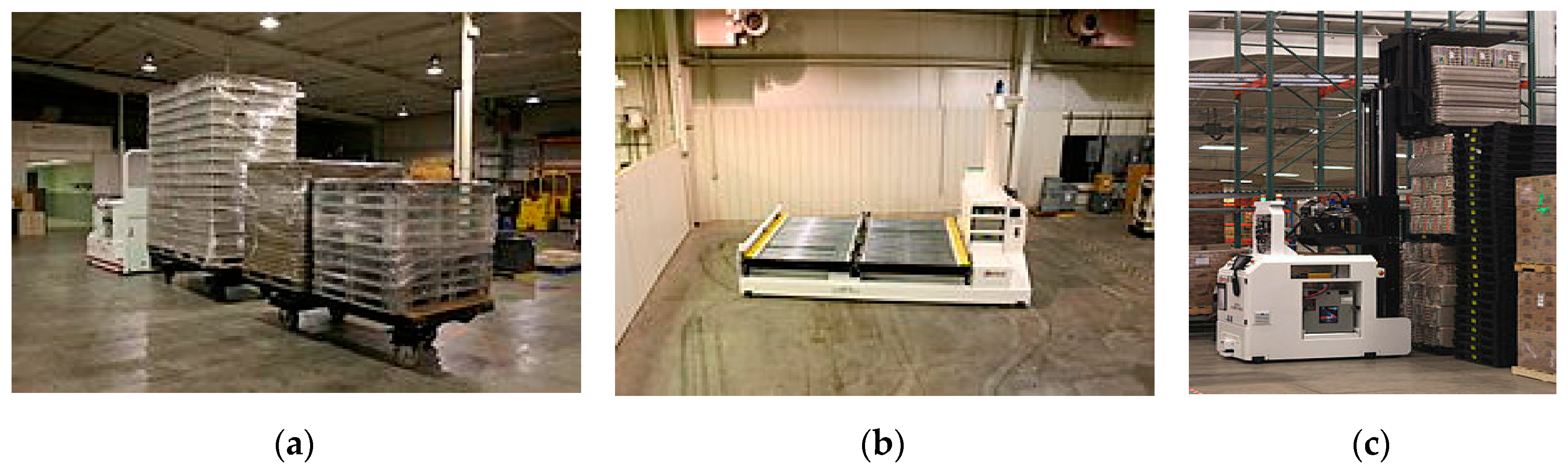
Typical features of AGV are related to the following parameters, as [5]:
  • weight and size,
  • load capacity (from a few kgs to several tons),
  • driving speed 1–2 m/s,
  • drive power,
  • navigation method, positioning accuracy,
  • time of loading and unloading,
  • battery capacity,
  • working time, battery charging time.
AGV uses electric drive and efficient batteries, however, it requires periodic recharging. Depending on the battery capacity and load, a typical work cycle includes 8–16 h of work and 4–8 h of battery charging, which takes place completely automatically. Some solutions for recharging the battery during short interruptions in the work of AGV (Opportunity Battery Charging) can be found. There are also solutions based on manual or automatic replacement of a depleted battery with a new fully charged battery (Battery Swap). This action takes about 10 min and allows to take full advantage of AGV’s working time but requires a more advanced service system and additional battery packs.
The design of a transport system based on AGVs requires an advanced navigation system and appropriate delineation of transport routes and reloading points. Based on the technique, various navigation systems are used, such as [37]:
  • photo-optical—with a passive lead line,
  • inductive—with an active lead line,
  • without a lead line—autonomous navigation with different location methods: incremental, infrared, ultrasonic, laser, gyroscopic, satellite (GPS).
Various methods can be used to design AGV systems, including mathematical programming methods, heuristic methods, Petri nets and computer simulations. These methods are used in order to improve the transport network in terms of criteria, for minimizing the length of transport routes, maximizing the production flow, scheduling transport tasks, number and location of transhipment points, parking zones and others [28,39].
Transport routes can be one- or two-way. Due to the reduction of the risk of collision, one-way roads in the form of closed loops, which enable cyclical transport operations, are the most commonly used [22]. In this case, it is easier to develop traffic control algorithms than in the case of two-way traffic, which requires additional passing and parking zones. Therefore, during the design of the AGV system, the most frequently used zones are defined including specific segments of the route (Segmented Flow Configuration) and individual transport loops (Single Loops) in a given segment. The advantages of such a solution are related to [40]:
  • All AGV vehicles move in the same direction, which practically excludes collisions,
  • system control is simplified due to the lack of alternative routes.
In turn, some drawbacks are connected with [35]:
  • Small fault tolerance, in the event of failure of one vehicle, the others usually cannot pass it by,
  • if the vehicle passes the given transfer point, it cannot turn back, but it must cross the entire loop once again to reach it again,
  • vehicles hold each other, which may lead to blockages of the system (deadlock).
When designing the AGV transport system, the most important problem is determining the number of vehicles needed to achieve the required production volume or the minimum number of vehicles required to obtain the optimal production volume [36,40].
There are a lot of situations in which the AGV system may stall because of a deadlock. A variety of deadlock-detecting algorithms are available in literature [41], but these methods work mainly for manufacturing system where the network layout is simple and uses only a small number of AGVs. The paper [42] discusses the development of an efficient strategy for predicting and avoiding the deadlocks in a large scale AGV systems. The integration of the scheduling of production and transport tasks tends to also be problematic because of computational complexity [43,44]. In initial papers, the transportation times between machines have not been considered. Their authors claimed that because transportation times are very small in comparison with the processing times, they are negligible [45]. On the other hand, in recent decades, the more researchers have been attracted by some issues that the transportation times were considerable and ignoring them can have impacts on the solution of scheduling problems.

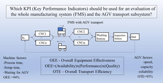
2.2. Evaluation of FMS and AGV

The performance of the AGV logistics system can have a great influence over the performance of the whole FMS system; therefore, a performance evaluation should be conducted. The key performance indicators (KPI) of the production system include [16,46]:
  • Production throughput,
  • time of the production process (Manufacturing Lead Time),
  • average waiting time for transport,
  • length of queues in storage buffers,
  • work in progress (WIP),
  • downtime of workstations,
  • delayed execution of production orders,
  • OEE—Overall Equipment Effectiveness,
  • OTE—Overall Throughput Effectiveness.
Work efficiency and the use of the means of production can be expressed by using the OEE metric that depends on three factors: availability, performance and quality [16].
OEE = ( Availability ) × ( Performance ) × ( Quality )
Availability is the ratio of the time spent on the realization of a task to the scheduled time. Availability is reduced by disruptions at work and machine failures.
Availability =   available   work   time failure   time scheduled   time
Machinery failures may cause severe disturbances in production processes and the loss of availability. Inherent availability can be calculated with Formula (3).
Availability =   MTBF MTBF + MTTR
where:
  • MTBF—Mean Time Between Failures,
  • MTTR—Mean Time To Repair.
The OEE metric was developed for single component maintenance. In the case of complex systems including serial or parallel subsystems the availability is changed. For the series system to be available, each subsystem should be available. For the parallel system to be available, whichever subsystem should be available.
Performance is the ratio of the time to complete a task under ideal conditions compared to the realization in real conditions; or the ratio of the products obtained in reality, to the number of possible products to obtain under ideal conditions. Performance is reduced (loss of working speed) by the occurrence of any disturbances, e.g., human errors.
Performance =   ideal   cycle   time real   cycle   time =   real   number   of   products ideal   number   of   products
Quality is expressed by the ratio of the number of good products and the total number of products.
Quality =   number   of   good   quality   products total   number   of   products
To compare the influence of the AGV logistic system over the manufacturing system, we will consider different OEE factors. However, according to the lean manufacturing paradigm, the flow of production through bottlenecks is the most important, therefore some equipment should be fully utilized whilst other equipment does not require full utilization. The literature review [16,46] indicates that OEE metrics are lacking at complex manufacturing systems and the factory level. In order to address this gap, an overall throughput effectiveness metric can be used [47]. It measures the factory-level performance and can also be used for performing factory-level diagnostics such as bottleneck detection and identifying hidden capacity. It also accounts for subsystems processing multiple products. Any factory layout can be modelled using a combination of the predefined subsystems (serial, parallel), which allows a determination of the Overall Factory Effectiveness (OFE). Note that the OEE equation can be further simplified as [46,47]:
OEE =   Actual   throughput   ( units )   from   equipment   in   total   time Theoretical   throughput   ( units )   from   equipment   in   total   time  
By extending this definition to the factory level, we have Overall Factory Effectiveness (OFE):
OFE =   Actual   throughput   ( units )   from   factory   in   total   time Theoretical   throughput   ( units )   from   factory   in   total   time
Similarly, the Overall Transport Effectiveness (OTE) can be defined:
OTE =   Actual   throughput   ( units )   from   vehicle   in   total   time Theoretical   throughput   ( units )   from   vehicle   in   total   time

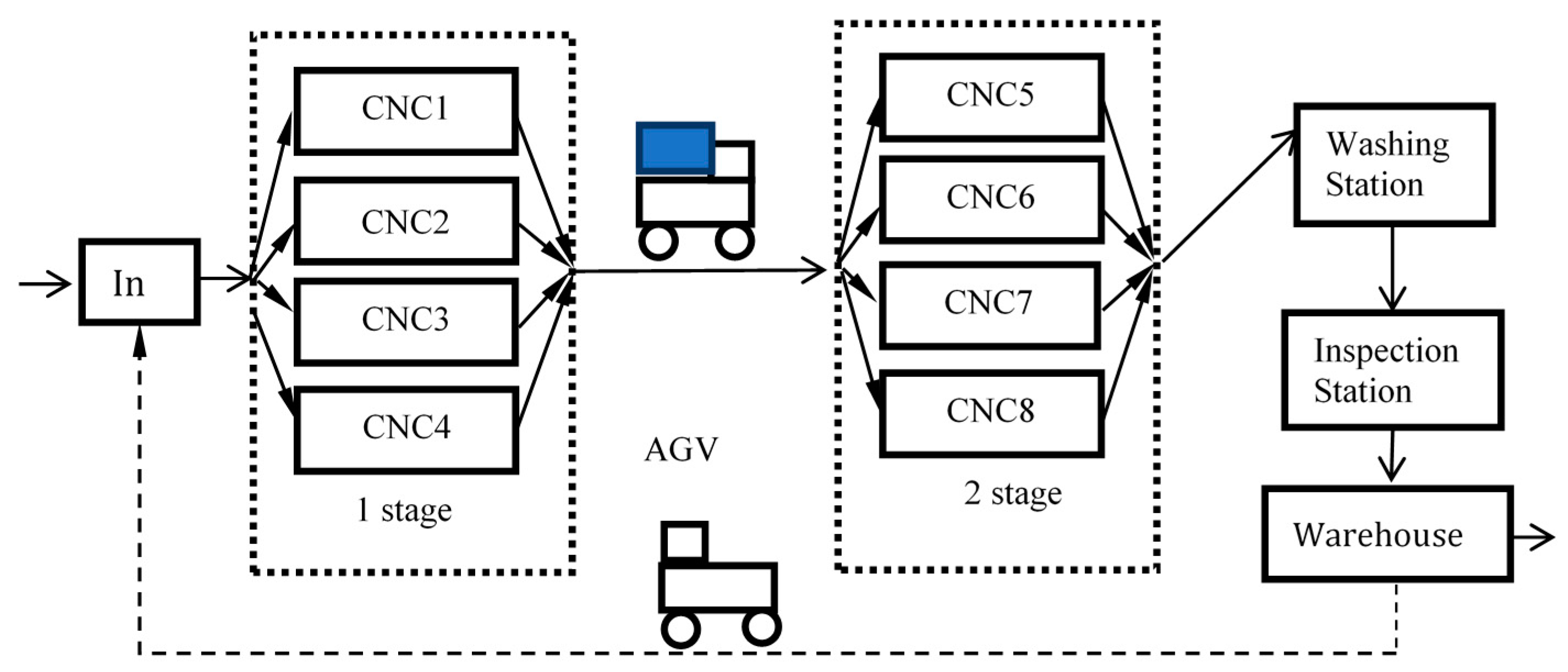
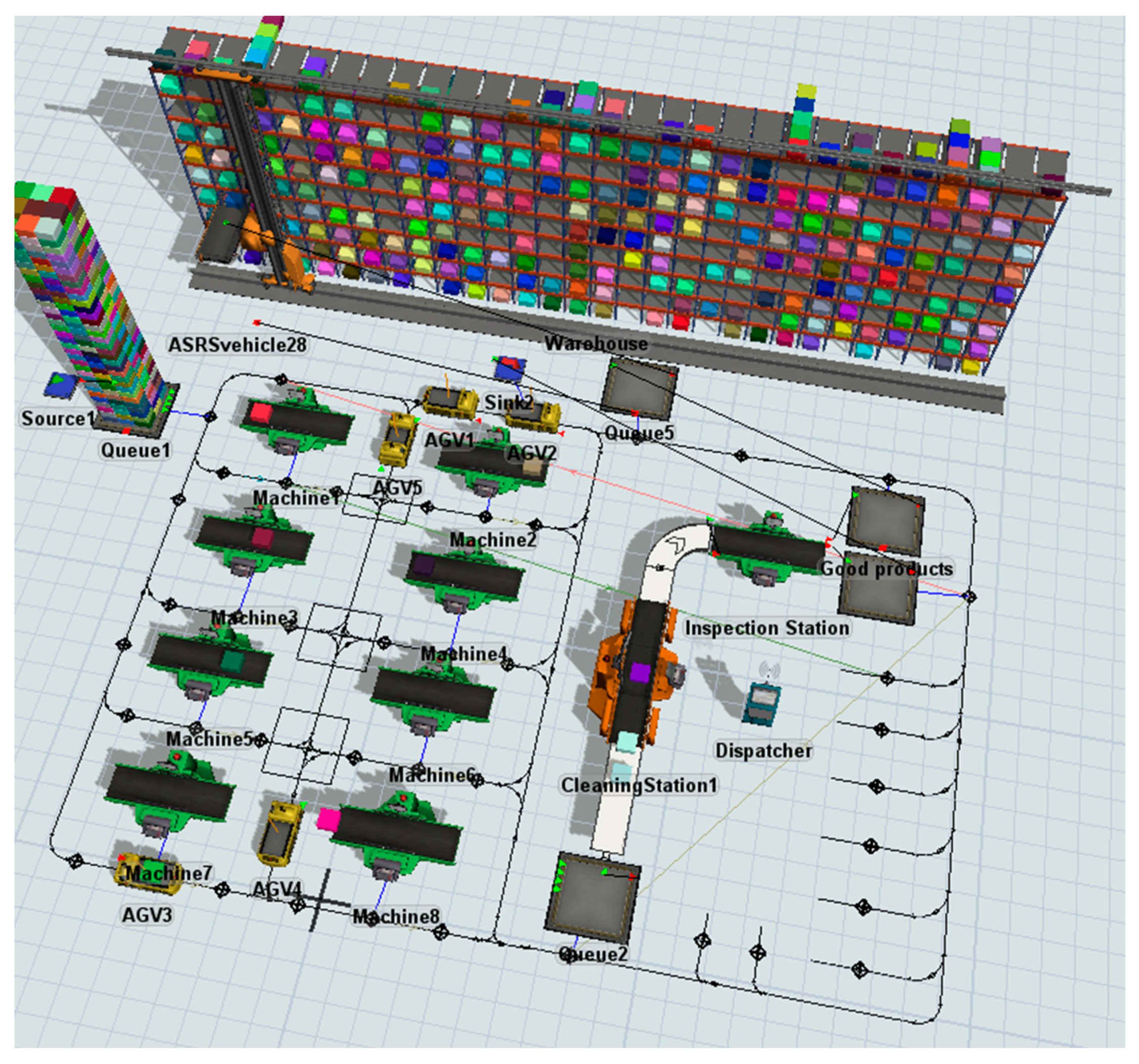
3. Description of the Problem—Materials and Methods

Let us consider a production system with eight automated machine tools, such as a CNC machining centre, which performs a two-stage process of machining a family of typical machine parts, like sleeves or discs of different sizes.
The machines are arranged as shown in Figure 2, which allows the series-parallel flow of production.
The system also includes an Automatic Washing Station and Inspection Station as well as a Storage System with an automatic rack stacker. Randomly generated various production orders are delivered to the system, differing in the duration of the operation (from 2.5 to 15.2 min). As a means of product transportation devices, several AGV vehicles are used, which will move along the planned transport routes. We assume that the manufacturing process meets the lean manufacturing, i.e., the flow of a single product and minimal buffers capacity to limit production in progress.
When designing a production system, we strive to achieve maximum production efficiency and, in particular, maximum utilization of machines and devices constituting bottlenecks in the manufacturing process. Other machines and devices will usually be used to a lesser extent, but they are necessary for the production process. By introducing changes to the model, we can analyse the formation of bottlenecks in the production system and their impact on the production volume. This allows, i.e., to determine the required storage capacity and capacity of the transport system. Particularly, the most interested issue is the impact of the number of AGV transport resources on the production efficiency of the entire system. For this purpose, a simulation model was developed in the FlexSim 2018 environment, shown in Figure 3.
Initially, the reference system consisted only of machines, without taking transport into account. It represents the manufacturing system in ideal conditions. At the next step, transport-related constraints were added to the model. The layout takes into account the dimensions of individual model objects and the distance between them. According to the recommendations given in the literature, the model uses unidirectional transport routes forming three main loops. Several control points have been introduced to designate places of loading and unloading as well as parking spaces. For the most used intersections, control zones were used to reduce the risk of collisions and blockages.
Typical parameters of AGV were assumed, including the speed of 2 m/s and a loading/unloading time of 30 s. A FIFO (First In First Out) control strategy was applied. In addition, the warehouse system was expanded by adding components such as the high storage warehouse with an automated storage retrieval system (ASRS).

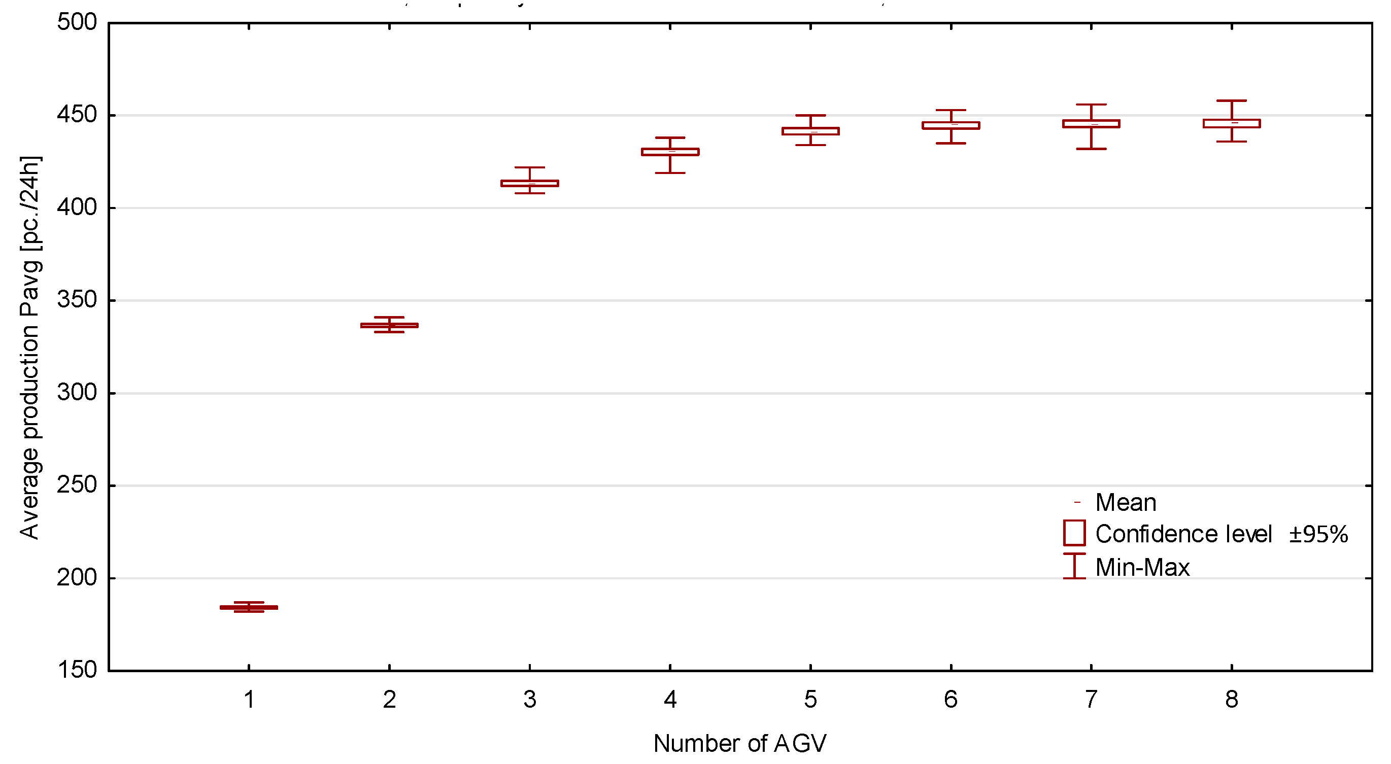
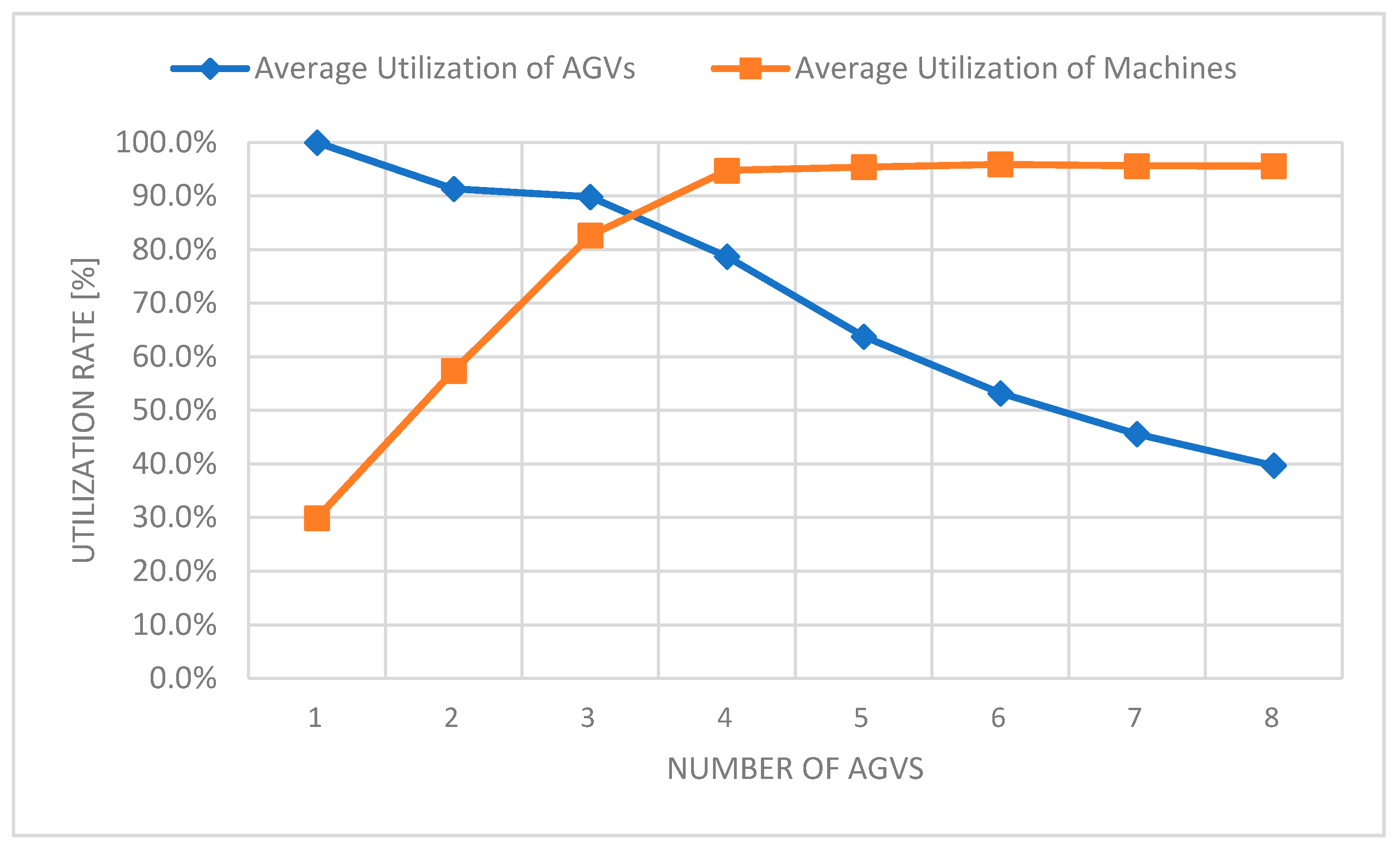
4. Results of the Simulation Experiments

The developed model was used to conduct a series of simulation experiments. In subsequent experiments, the number of AGV vehicles from 0 to 8 was changed. The simulation time of 24 h was assumed as the time of automatic maintenance of the entire system. A random generation of production orders was assumed according to the exponential distribution with the expected value of 100 s. As a result of a lack of data and the need for simplification, the retooling of the system, charging of AGV batteries and the failure of machines and vehicles was omitted. As part of each experiment, 30 simulation runs were carried out. The results are presented in Table 1 and Figure 4, respectively. Due to the stochastic parameters of the model, the production value Pavg obtained in the experiment is a random variable with a distribution close to normal.
The first row in the Table 1, where the number of AGV amount is 0, represents the reference system consisting only of machines and not taking transport into account (transport time equal to zero).
Figure 4 presents the relationship between average production Pavg and the number of AGVs used for transport in the form of a box-and-whisker plot.
The box represents a 95% confidence interval, which means the average production volume is within this range with a probability of 95%, whilst, whiskers represent the maximum and minimum value of production obtained in a given experiment (there is a small spread of results, therefore some of the boxes in the chart are very small).
In the Figure 4, it can be seen that initially the increase of the AGV number results in a rapid increase of obtained production volume. On the other hand, increasing the AGVs number above 5 units results in a slight increase in production, as more vehicles are used to a lesser extent. A similar phenomenon is described in the literature [36] as the effect of the mutual blocking of AGVs.
To eliminate them, it would be necessary to use multi-lane transport routes or passages. The excessive increase in the number of AGVs is in turn associated with high costs and brings little effects and a relatively small increase in production efficiency [34] with a drop in the effectiveness of AGV being used.
The comparison with the results obtained in the ideal conditions (AGV = 0, Pavg = 561 pc.) shows a great difference with the other results. For example, for 5 AGVs system, there was a Pavg = 441.5 pc., average machine utilization of about 70% and average AGVs utilization of about 50% (from the range of 28–71% for AGV1 and AGV5). The increase of the AGV number caused very little increase in machine utilization and a considerable decrease in the utilization of the additional AGVs.
That problem requires a more detailed investigation, but the traditional metrics for measuring productivity as throughput or utilization rate are not very helpful for identifying the problems and underlying improvements needed to increase productivity. In this situation, a more rigorously defined productivity metric is needed [44]. Therefore, in this case, OEE metrics can be used, which take into account equipment availability, breakdowns, performance (reduced speed, idling) and quality (good and bad quality products).

Second Experiment

A more detailed model of the FMS system was developed taking into account the quality, availability and reliability of AGVs and battery charging.
AGVs have very advanced design and are considered very reliable, but there are certainly few publications about AGV reliability, compared to publications about machine reliability including [48,49]. With the use of fault tree analysis, a reliability block diagram and a hazard decision tree of AGV components, reliability evaluation of the failure rate λ [1/h] was estimated to be 0.003 [48] and 0.0014 [49]. That can also be described with the Mean Time Between Failures (MTBF) as reciprocal of the failure rate λ. Basing on the λ values, we have the range of MTBF = 300 ÷ 700 h and we have assumed an average of MTBFagv = 500 h for modelling the reliability of AGV. We have also assumed Mean Time To Repair (MTTRagv) = 8 h. The reliability of CNC machine tools was omitted because its reliability should be much better than that of AGVs, and we will concentrate on the failure effect of the AGVs. The machines are working parallelly; therefore, the effect of machine failures would be very small. On the other hand, another random factor could hinder the analysis of results.
The AGV can work 24 h per day but sometimes battery loading is required. We have assumed a working schedule for 6 AGVs with a 4 h pause for battery loading. It means that AGVs charge the batteries alternately, and in each moment 5 AGVs are working and one is charging the battery. In the case of malfunction, the AGV is automatically moving to the parking place for maintenance or should be manually removed to prevent blockage.
The scenario includes continuous work of the FMS for 3 shifts per day and 5 days per week. As a result of the long-time effect of AGVs failures, long-time simulations were performed, including work for 24, 120, 500 and 1500 h. The experiment’s results without and with reliability parameters of AGVs are presented in Table 2 and Table 3, respectively. (The raw data are included in the Supplementary Materials).
An analysis of the previous model showed that blockage of the machines sometimes occurs; therefore, small loading/unloading buffers with a capacity of one piece were added to machines in order to improve the production flow. Quality parameters were defined as 99.9% of good products according to the OEE quality factor.
Comparing the results from Table 2 and Table 3, a small but significant effect of AGVs failures on production can be seen (a decrease of about 0.7%). For a more detailed analysis, the OFE metrics can be used. Since the model was built based on the OEE components and contains parameters of availability, performance and quality, the production value from the simulation Pavg can be directly used to calculate the OFE indicator [25,41].
OFE = P avg P limit
The value Plimit represents the theoretically available maximal production in ideal conditions. For the average machining time of tm = 530 s, the limit is equal to 6.79 pc./hour for one machine and 652 pc./24 h for the whole machining system (Plimit = 27.17 pc./hour).
The juxtaposition of the OFE indexes is included in Table 4.
The differences between OFE2 and OFE3 are related to the warmup of the system in a short time and to the effect of AGV failures in a long time. This result is consistent with assumed reliability parameters and inherent availability (Equation (3)) of AGV and parallel system. As there is a small probability of simultaneous failure of all AGVs, the effect is connected with the loss of performance including loss of speed during loading/unloading, waiting for transport and blocking.

5. Discussion

The question is—which KPI should be used for an evaluation of the whole manufacturing system and the transport subsystem?
The key factor is the production flow through the machines, as there is the bottleneck, which is related with the utilization of the machines and transport vehicles.
The relationship between average utilization of machines and AGVs and the number of AGVs used for 24 h of simulation is shown in the Figure 5. With the increasing number of AGVs, the utilization of machines is increasing, and at the same time the utilization of vehicles is decreasing. These two performance goals are mutually exclusive. The maximum average machine utilization was about 95% compared to about 53% for 6 AGVs (from the range 46–62%).
We propose an analysis of the effectiveness of the transport system by the Overall Transport Effectiveness (OTE) metric that can be determined on the basis of the number of transport operations carried out and the theoretical planned limit of transport operations per vehicle. There are 4 transport operations for each product in the production flow, therefore, the production of Plimit = 652 products requires AGVlimit = 2608 transport operations. One AGV can make about 782 transport operations during 24 h. As the AGVs are working parallelly, then theoretically the 3.3 AGVs should be enough, but if there are more vehicles the blocking can occur more frequently. Therefore, the overall transport effectiveness per vehicle was also calculated and is presented in the Table 5.
There is a close relationship between the number of achieved products and the number of required transport operations. However, there is a small difference in the values of OFE and OTE, because of work in progress and related transport operations. The value of OTE is depended on the number of AGVs. The maximal value of OTE = 95.737% (±0.25%) was achieved for 6 AGVs. In the case of battery charging, the value of OTE = 95.621% was achieved. The failures have decreased the value by about 0.27% to OTE = 95.353%.
However, for longer simulation time, the system is more stable and a maximal value of OFE = 96.076% and OTE = 96.194% was achieved for the longest simulation time of 1500 h.
It should be noted that there can be different versions of the OTE metric due to the scope of the data taken into account. The main difference in this version is that only planned transport operations are taken into consideration (not all possible working time as in utilization rate).
According to principles of lean manufacturing, an unnecessary movement of people, information or materials wastes time and increases costs. Any unnecessary transport of raw materials in the plant is a waste, and thus should be reduced.
Any non-critical resource such as AGV should be “utilized”, such that the bottleneck is never starved for work and all work that is processed by the bottleneck is of high quality. Otherwise, additional activation of these resources just generates excess work-in-process and additional costs. This condition will be met if the OTE is greater than or equal to OEE (OFE).
OTE ≥ OEE (OFE)
Therefore, the hypothesis that there is dependence between plant effectiveness and transport effectiveness, which can be expressed by the use of the OEE metric, has been proven.
In the case of other logistics systems (e.g., transport of multiple products, different routes with returns), the difference in value between OFE and OTE may be greater. These problems and industrial implementation of the proposed methodology in the context of the digital twin for Industry 4.0, will be taken into account in further research.

6. Conclusions

Due to the complexity of AGV systems, they cause many decision problems, which are difficult to solve. The paper has presented an example of the Flexible Manufacturing System solution with the AGV transport system and discusses some issues related to the design and simulation of such systems. The stage of initial system design optimization is very important, and computer simulation enables the relatively easy elaboration and testing of various variants of manufacturing and logistics systems. On the other hand, excessive simplifications may be applied at the modelling stage, which will make the simulation not reflect the production system properly. It should be noted that detailed modelling is very labour intensive and requires the involvement of experienced specialists. Therefore, choosing what parameters are used in the modelling process and which metric is used to evaluate the model is very important. In order to make the simulation more accurate and to evaluate the system’s productivity, the use of Overall Equipment Effectiveness (OEE) metrics was proposed.
The results obtained from the presented simulations show that the OEE metrics can be used for the modelling and productivity evaluation of manufacturing and logistics systems, with the generalization of Overall Factory Effectiveness (OFE) and Overall Transport Effectiveness (OTE). The use of OEE factors also allows to compare the results obtained from different manufacturing systems. In the real world, most of manufacturing companies have OEE scores closer to 60%, but there are many of them with OEE scores lower than 45%, and a small number of world-class companies that have the OEE value higher than 85% [50]. According to that, the results of simulation can be also used to analyse the costs involved in the implementation of a given project and at the stage of in-depth design of the production system.

Supplementary Materials

Author Contributions

Conceptualization, A.K. and G.G.; methodology, A.K.; validation, K.F., G.G.; investigation, K.F.; data curation, G.G.; writing—original draft preparation, A.K.; visualization, G.G. All authors have read and agreed to the published version of the manuscript.

Funding

This research received no external funding.

Conflicts of Interest

The authors declare no conflict of interest.

References

  1. Rutner, S.M.; Langley, C.J. Logistics Value: Definition, Process and Measurement. Int. J. Logist. Manag. 2000, 11, 73–82. [Google Scholar] [CrossRef]
  2. Schuhmacher, J.; Baumung, W.; Hummel, V. An Intelligent Bin System for Decentrally Controlled Intralogistic Systems in Context of Industrie 4.0. Procedia Manuf. 2017, 9, 135–142. [Google Scholar] [CrossRef]
  3. Paszkiewicz, A.; Bolanowski, M.; Budzik, G.; Przeszłowski, Ł.; Oleksy, M. Process of Creating an Integrated Design and Manufacturing Environment as Part of the Structure of Industry 4.0. Processes 2020, 8, 1019. [Google Scholar] [CrossRef]
  4. Avelar-Sosa, L.; Alcaraz, J.L.G.; Maldonado-Macías, A.A.; Mejía-Muñoz, J. Application of structural equation modelling to analyse the impacts of logistics services on risk perception, agility and customer service level. Adv. Prod. Eng. Manag. 2018, 13, 179–192. [Google Scholar] [CrossRef] [Green Version]
  5. Berman, S.; Schechtman, E.; Edan, Y. Evaluation of automatic guided vehicle systems. Robot. Comput. Manuf. 2009, 25, 522–528. [Google Scholar] [CrossRef]
  6. De Ryck, M.; Versteyhe, M.; DeBrouwere, F. Automated guided vehicle systems, state-of-the-art control algorithms and techniques. J. Manuf. Syst. 2020, 54, 152–173. [Google Scholar] [CrossRef]
  7. Kampa, A.; Golda, G.; Paprocka, I. Discrete Event Simulation Method as a Tool for Improvement of Manufacturing Systems. Computers 2017, 6, 10. [Google Scholar] [CrossRef]
  8. Kampa, A.; Gołda, G. Modelling and simulation method for production process automation in steel casting foundry. Arch. Foundry Eng. 2018, 18, 47–52. [Google Scholar] [CrossRef]
  9. Barosz, P.; Golda, G.; Kampa, A. Efficiency Analysis of Manufacturing Line with Industrial Robots and Human Operators. Appl. Sci. 2020, 10, 2862. [Google Scholar] [CrossRef] [Green Version]
  10. Lambert, D.M.; Burduroglu, R. Measuring and Selling the Value of Logistics. Int. J. Logist. Manag. 2000, 11, 1–18. [Google Scholar] [CrossRef]
  11. Lynch, D.; Keller, S.; Ozment, J. The effects of logistics capabilities and strategy on firm performance. J. Bus. Logist. 2000, 21, 47–67. [Google Scholar]
  12. Griffis, S.E.; Cooper, M.; Goldsby, T.J.; Closs, D.J. Performance Measurement: Measure Selection Based upon Firm Goals and Information Reporting Needs. J. Bus. Logist. 2004, 25, 95–118. [Google Scholar] [CrossRef]
  13. Fugate, B.S.; Mentzer, J.T.; Stank, T.P. Logistics Performance: Efficiency, Effectiveness, and Differentiation. J. Bus. Logist. 2010, 31, 43–62. [Google Scholar] [CrossRef]
  14. Lambert, D.M.; Pohlen, T.L. Supply Chain Metrics. Int. J. Logist. Manag. 2001, 12, 1–19. [Google Scholar] [CrossRef]
  15. Muthiah, K.M.; Huang, S.H. A review of literature on manufacturing systems productivity measurement and improvement. Int. J. Ind. Syst. Eng. 2006, 1, 461. [Google Scholar] [CrossRef] [Green Version]
  16. Roda, I.; Macchi, M. Factory-level performance evaluation of buffered multi-state production systems. J. Manuf. Syst. 2019, 50, 226–235. [Google Scholar] [CrossRef]
  17. Andersson, C.; Bellgran, M. On the complexity of using performance measures: Enhancing sustained production improvement capability by combining OEE and productivity. J. Manuf. Syst. 2015, 35, 144–154. [Google Scholar] [CrossRef]
  18. Muñoz-Villamizar, A.; Santos, J.; Montoya-Torres, J.R.; Jaca, C. Using OEE to evaluate the effectiveness of urban freight transportation systems: A case study. Int. J. Prod. Econ. 2018, 197, 232–242. [Google Scholar] [CrossRef]
  19. Dalmolen, S.; Moonen, H.; Iankoulova, I.; Van Hillegersberg, J.; Simon, D.; Hans, M.; Iliana, I.; Jos, V.H. Transportation Performances Measures and Metrics: Overall Transportation Effectiveness (OTE): A Framework, Prototype and Case Study. Proc. Annu. Hawaii Int. Conf. Syst. Sci. 2013, 4186–4195. [Google Scholar] [CrossRef]
  20. McCalion, R. Is OEE relevant to lift truck fleet & warehouse operations? Eureka 2013. Available online: https://eurekapub.eu/fleet-management/2013/09/14/fleet-management (accessed on 26 September 2020).
  21. Hayes, J. AGV IIoT Monitoring: Lean Six Sigma Monitoring. RFID J. 2018. Available online: https://www.rfidjournal.com/agv-iiot-monitoring-lean-six-sigma-monitoring-2 (accessed on 27 September 2020).
  22. Palací-López, D.; Borràs-Ferrís, J.; Oliveria, L.T.D.S.D.; Ferrer-Riquelme, A.J. Multivariate Six Sigma: A Case Study in Industry 4.0. Process 2020, 8, 1119. [Google Scholar] [CrossRef]
  23. Golda, G.; Kampa, A.; Foit, K. Study of inter-operational breaks impact on materials flow in flexible manufacturing system. IOP Conf. Ser. Mater. Sci. Eng. 2018, 400, 022030. [Google Scholar] [CrossRef]
  24. Alzubi, E.; Atieh, A.M.; Abu Shgair, K.; Damiani, J.; Sunna, S.; Madi, A. Hybrid Integrations of Value Stream Mapping, Theory of Constraints and Simulation: Application to Wooden Furniture Industry. Process 2019, 7, 816. [Google Scholar] [CrossRef] [Green Version]
  25. Zhang, X.; Li, Y.; Ran, Y.; Zhang, G. Stochastic models for performance analysis of multistate flexible manufacturing cells. J. Manuf. Syst. 2020, 55, 94–108. [Google Scholar] [CrossRef]
  26. Hoshino, S.; Ota, J.; Shinozaki, A.; Hashimoto, H. Hybrid Design Methodology and Cost-Effectiveness Evaluation of AGV Transportation Systems. IEEE Trans. Autom. Sci. Eng. 2007, 4, 360–372. [Google Scholar] [CrossRef]
  27. Um, I.; Cheon, H.; Lee, H. The simulation design and analysis of a Flexible Manufacturing System with Automated Guided Vehicle System. J. Manuf. Syst. 2009, 28, 115–122. [Google Scholar] [CrossRef]
  28. Vis, I.F. Survey of research in the design and control of automated guided vehicle systems. Eur. J. Oper. Res. 2006, 170, 677–709. [Google Scholar] [CrossRef]
  29. Yan, R.; Dunnett, S.J.; Jackson, L. Novel methodology for optimising the design, operation and maintenance of a multi-AGV system. Reliab. Eng. Syst. Saf. 2018, 178, 130–139. [Google Scholar] [CrossRef]
  30. Florescu, A.; Barabas, S.A. Modeling and Simulation of a Flexible Manufacturing System—A Basic Component of Industry 4.0. Appl. Sci. 2020, 10, 8300. [Google Scholar] [CrossRef]
  31. Deroussi, L. Flexible Manufacturing Systems: Metaheuristics Logist; Wiley: Hoboken, NJ, USA, 2016; pp. 143–160. [Google Scholar] [CrossRef]
  32. Tolio, T. (Ed.) Design of Flexible Production Systems: Methodologies and Tools; Springer: Berlin, Germany, 2009. [Google Scholar] [CrossRef]
  33. Banks, J.; Nelson, B.L.; Carson, J.S.; Nicol, D.M. Discrete-Event System Simulation. Technometrics 1984, 26, 195. [Google Scholar] [CrossRef]
  34. Burduk, A. Stability Analysis of the Production System Using Simulation Models. In Process Simulation and Optimization in Sustainable Logistics and Manufacturing; Pawlewski, P., Greenwood, A., Eds.; Springer Science and Business Media LLC: Cham, Switzerland, 2014; pp. 69–83. [Google Scholar]
  35. Plaia, A.; Lombardo, A.; Nigro, G.L. Robust Design of Automated Guided Vehicles System in an FMS. In Advanced Manufacturing Systems and Technology; Kuljanic, E., Ed.; Springer: Vienna, Austria, 1996; pp. 259–266. [Google Scholar]
  36. A Vis, I.F.; De Koster, R.; Roodbergen, K.J.; Peeters, L.W.P. Determination of the number of automated guided vehicles required at a semi-automated container terminal. J. Oper. Res. Soc. 2001, 52, 409–417. [Google Scholar] [CrossRef]
  37. Qi, M.; Li, X.; Yan, X.; Zhang, C. On the evaluation of AGVS-based warehouse operation performance. Simul. Model. Pract. Theory 2018, 87, 379–394. [Google Scholar] [CrossRef]
  38. Automated Guided Vehicle. Wikipedia. Available online: https://en.wikipedia.org/wiki/Automated_guided_vehicle (accessed on 30 September 2020).
  39. Nieoczym, A.; Tarkowski, S. The modeling of the assembly line with a technological automated guided vehicle (AGV). LogForum 2011, 7, 35–42. [Google Scholar]
  40. Vivaldini, K.C.T.; Rocha, L.F.; Martarelli, N.J.; Becker, M.; Moreira, A.P. Integrated tasks assignment and routing for the estimation of the optimal number of AGVS. Int. J. Adv. Manuf. Technol. 2016, 82, 719–736. [Google Scholar] [CrossRef]
  41. Li, Z.; Wu, N.; Zhou, M. Deadlock Control of Automated Manufacturing Systems Based on Petri Nets—A Literature Review. IEEE Trans. Syst. Man. Cybern. Part C Appl. Rev. 2011, 42, 437–462. [Google Scholar] [CrossRef]
  42. Moorthy, R.L.; Hock-Guan, W.; Wing-Cheong, N.; Chung-Piaw, T. Cyclic deadlock prediction and avoidance for zone-controlled AGV system. Int. J. Prod. Econ. 2003, 83, 309–324. [Google Scholar] [CrossRef]
  43. Lv, Y.L.; Zhang, G.; Zhang, J.; Dong, Y.J. Integrated Scheduling of the Job and AGV for Flexible Manufacturing System. Appl. Mech. Mater. 2011, 80, 1335–1339. [Google Scholar] [CrossRef]
  44. Mousavi, M.; Yap, H.J.; Musa, S.N.; Tahriri, F.; Dawal, S.Z.M. Multi-objective AGV scheduling in an FMS using a hybrid of genetic algorithm and particle swarm optimization. PLoS ONE 2017, 12, e0169817. [Google Scholar] [CrossRef] [Green Version]
  45. Saidi-Mehrabad, M.; Dehnavi-Arani, S.; Evazabadian, F.; Mahmoodian, V. An Ant Colony Algorithm (ACA) for solving the new integrated model of job shop scheduling and conflict-free routing of AGVs. Comput. Ind. Eng. 2015, 86, 2–13. [Google Scholar] [CrossRef]
  46. Muthiah, K.M.N.; Huang, S.H. Overall throughput effectiveness (OTE) metric for factory-level performance monitoring and bottleneck detection. Int. J. Prod. Res. 2007, 45, 4753–4769. [Google Scholar] [CrossRef]
  47. Huang, S.H.; Dismukes, J.P.; Shi, J.; Su, Q.; Razzak, M.A.; Bodhale, R.; Robinson, D.E. Manufacturing productivity improvement using effectiveness metrics and simulation analysis. Int. J. Prod. Res. 2003, 41, 513–527. [Google Scholar] [CrossRef]
  48. Fazlollahtabar, H.; Saidi-Mehrabad, M. Autonomous Guided Vehicles; Springer Science and Business Media LLC: Cham, Switzerland, 2015; Volume 20. [Google Scholar]
  49. Yan, R.; Jackson, L.; Dunnett, S.J. Automated guided vehicle mission reliability modelling using a combined fault tree and Petri net approach. Int. J. Adv. Manuf. Technol. 2017, 92, 1825–1837. [Google Scholar] [CrossRef] [Green Version]
  50. OEE Benchmark Study. Available online: https://sageclarity.com/articles-oee-benchmark-study (accessed on 28 September 2020).
Figure 1. Examples of Automated Guided Vehicles (AGVs), (a) pulling trailers with cargo, (b) transporting pallets, (c) lifting loads with a forklift [38].
Processes 08 01648 g001
Figure 2. The schema of Flexible Manufacturing System (FMS) with AGV transport.
Processes 08 01648 g002
Figure 3. Simulation model of the FMS with AGV transport.
Processes 08 01648 g003
Figure 4. The relationship between average production Pavg and the number of AGV used for 24 h of simulation.
Processes 08 01648 g004
Figure 5. The relationship between average utilization of machines and AGVs and the number of AGV used for 24 h of simulation.
Processes 08 01648 g005
Table 1. The results of simulation experiments (Average production completed Pavg, in [pieces] for 24 h of work, 30 simulation runs in each experiment, 95% confidence level).
Number of AGVs
NAGV
Minimum
Production
Pmin
[Pieces]
Lower Limit of 95% Confidence Interval
[Pieces]
Average production
Pavg
[Pieces]
Upper Limit of 95% Confidence Interval
[Pieces]
Maximum
Production
Pmax
[Pieces]
Standard Deviation
Σ
0548559.05615635736.3
1182183.66184.7184.871871.62
2333335.97336.7337.433411.95
3408412.1413.4414.74223.6
4419428.6430.34324384.5
5434439.8441.5443.34504.7
6435443.0444.7446.44534.6
7432443.8445.6447.44564.9
8436443.6445.7447.84585.6
Table 2. The results of simulation experiments (Average production completed Pavg, in [pieces] for 6 AGVs with battery charging, without failures, 30 simulation runs in each experiment, 95% confidence level).
Time
[Hours]
Minimum
Production
Pmin
[pc.]
Lower Limit of 95%
Confidence Interval
[pc.]
Average Production
Pavg
[pc.]
Upper Limit of 95%
Confidence Interval
[pc.]
Maximum
Production
Pmax
[pc.]
Standard Deviation
σ
Average Throughput
[pc./Hour]
24593611614.2617.56348.725.59
12030943131.83139.93148.1318821.826.17
50013,06113,116.713,128.313,139.913,18831.126.26
150039,28839,38739,40639,42539,5345126.27
Table 3. The results of simulation experiments (Average production completed Pavg, in [pieces] for 6 AGVs with battery charging, with AGVs failures, MTBF = 500 h, MTTR = 8 h, 30 simulation runs in each experiment, 95% confidence level).
Time
[Hours]
Minimum
Production
Pmin
[pc.]
Lower Limit of 95%
Confidence Interval
[pc.]
Average Production
Pavg
[pc.]
Upper Limit of 95%
Confidence Interval
[pc.]
Maximum
Production
Pmax
[pc.]
Standard Deviation
σ
Average Throughput
[pc./Hour]
24549607.3613.2618.363414.825.55
120281030913116314131746825.97
50012,32712,96513,03013,09413,16217326.06
150038,40239,04439,15139,25839,46328726.10
Table 4. The Overall Factory Effectiveness (OFE) metrics for model of 6 AGVs without failures OFE2 and with failures OFE3 and OFE1 from the previous experiment.
Time
[Hours]
PlimitPavg1OFE1Pavg2OFE2Pavg3OFE3
24652444.70.68206614.20.94203613.20.94049
12032602252.30.690893139.90.9631631160.95583
50013,583.339407.60.6925813,128.30.9665013,0300.95926
150040,75028,230.70.6927839,4060.9670239,1510.96076
Table 5. OTE—Overall Transport Effectiveness and OFE—Overall Factory Effectiveness (24 h of simulation, 30 simulation runs in each experiment, without failures and battery charging).
Nr of AGVs
Nagv
Plimit
[Pc.]
AGVlimit
(4 × Plimit/Nagv)
[Pc.]
Pavg
[pc.]
Finished
Transport Operation
[pc.]
Average Transport
Oper./AGV
[pc.]
OTEOFE
16522608186.7781.9781.90.299810.28635
26521304347.231428.2714.10.547620.53256
3652869.3516.72107.5702.50.808120.79249
4652652.0606.02461.4615.40.943790.92945
5652521.6614.02493.0498.60.955900.94172
6652434.7615.02497.0416.20.957370.94325
7652372.6614.02494.4356.30.956370.94172
8652326.0611.72484.5310.60.952650.93819
Publisher’s Note: MDPI stays neutral with regard to jurisdictional claims in published maps and institutional affiliations.

