Quality-Relevant Monitoring of Batch Processes Based on Stochastic Programming with Multiple Output Modes


1
School of Information Science and Engineering, Zhejiang University Ningbo Institute of Technology, Ningbo 315100, China
2
School of Mechanical Engineering and Automation, College of Science & Technology Ningbo University, Ningbo 315300, China
3
College of Computer Internet of Things Engineering, Jiangnan University, Wuxi 214122, China
*
Authors to whom correspondence should be addressed.
Processes 2020, 8(2), 164; https://0-doi-org.brum.beds.ac.uk/10.3390/pr8020164
Submission received: 27 December 2019
/
Revised: 31 January 2020
/
Accepted: 1 February 2020
/
Published: 2 February 2020
(This article belongs to the Special Issue Modeling, Control, and Optimization of Batch and Batch-Like Processes)
Abstract
:To implement the quality-relevant monitoring scheme for batch processes with multiple output modes, this paper presents a novel methodology based on stochastic programming. Bringing together tools from stochastic programming and ensemble learning, the developed methodology focuses on the robust monitoring of process quality-relevant variables by taking the stochastic nature of batch process parameters explicitly into consideration. To handle the problem of missing data and lack of historical batch data, a bagging approach is introduced to generate individual quality-relevant sub-datasets, which are used to construct the corresponding monitoring sub-models. For each model, stochastic programming is used to construct an optimal quality trajectory, which is regarded as the reference for online quality monitoring. Then, for each sub-model, a corresponding control limit is obtained by computing historical residuals between the actual output and the optimal trajectory. For online monitoring, the current sample is examined by all sub-models, and whether the monitoring statistic exceeds the control limits is recorded for further analysis. The final step is ensemble learning via Bayesian fusion strategy, which is under the probabilistic framework. The implementation and effectiveness of the developed methodology are demonstrated through two case studies, including a numerical example, and a simulated fed-batch penicillin fermentation process.
1. Introduction
1.1. Background and Literature Review
Batch processes are widely used in modern industrial applications due to the growing requirements of producing high-value products, such as food, plastics, pharmaceuticals, and biological and semiconductor materials [1,2,3,4]. Since the products of batch processes often require extremely high quality, the problem of quality-relevant monitoring has received increased attention in recent years. The concept of “quality-relevant” monitoring—also known as “output-relevant” monitoring—was proposed [5,6,7] to describe output-relevant faults that directly affect process quality, which is captured by the output variables. It is important to develop output-relevant monitoring methods for process safety and quality enhancement in batch processes. Over the past few decades, various approaches have been proposed to solve the problem using multivariate statistical process monitoring (MSPM) methods, such as multiway principal component analysis (MPCA) and multiway partial least squares (MPLS) [8,9]. These traditional data-based methods are developed for monitoring purposes based on historical batch data [10,11]. Other approaches have also been proposed for quality-relevant monitoring of batch processes to improve performance [12,13]. However, with the increased complexity and integrated nature of modern industrial processes, the quality variables of different batches may behave rather differently, primarily due to the stochastic nature of process parameters and other process uncertainties.
Although existing methods can meet regular monitoring requirements, difficulties arising from practical implementation considerations in industrial batch process operations need to be addressed and accounted for explicitly in the monitoring method development. The lack of historical data, for example, is an important problem that is encountered when data-based modeling is implemented. This problem is commonly the result of the missing data problem, the insufficiency of historical batches, and the lack of quality variables [14,15]. There are two major problems related to missing data: one is missing measurements in historical data, and the other is missing observations in online data [16]. In most existing research works on the missing data problem, the focus has been more on the missing observations, since offline model construction is made under the assumption that abundant historical data have been acquired [17,18,19,20]. Meanwhile, insufficient batches are usually ignored for the same reason. To deal with the problem of historical missing data, simple imputation (such as using mean values of nearby samples) is used widely to fill missing elements. Furthermore, for most data-driven monitoring methods for batch processes, quality variables are considered difficult to obtain. Thus, soft-sensor methods, such as multi-block/multi-way partial least squares [21], are proposed to make use of the limited quality data. As a result, it is necessary to deal with the deficiency in historical data to construct more reliable offline models. While some data-based methods have been proposed to handle these problems, the stochastic nature of batch processes is often ignored since the physico-chemical mechanism underlying the process is not considered in data-based methods. It is therefore expected that combining the mechanistic knowledge of the process together with the data collected from process sensors will aid in developing a robust monitoring model. However, one is typically faced with the challenge that the entire mechanism or the first-principles model of a process is difficult to obtain, which is one of the limitations of model-based monitoring methods. As a result, a feasible compromise is to use process data together with only partial process knowledge to construct a quality-relevant monitoring model [22,23].
1.2. Research Motivation and Purpose
As is known to us, batch process monitoring is a necessary task in the modern industry. Due to the increasing complexity of practical batch processes, monitoring methods under the assumption that the process feature is simple and ideal can no longer provide accurate and robust monitoring results. Although the relevant literatures can handle part of the difficulties for batch process monitoring mentioned above, the monitoring problem of complex batch processes with multiple output modes is still a difficult task to accomplish. Process stochastics and uncertainties, as well as the lack of modeling data, and the insufficiency of historical batches, are crucial issues in the modeling procedure of complex batch processes, resulting in unreliable monitoring accuracy and robustness.
To address the aforementioned challenges, we draw extreme attention to the monitoring scheme of complicated batch processes with multiple output modes. With the combination of stochastic programming and an ensemble learning strategy, an integrated individual monitoring framework can solve some of the important issues pertaining to complicated batch process monitoring (e.g., multi-output modes and data deficiency of historical data).
Stochastic programming is the core method to achieve robust modeling and monitoring in the proposed monitoring framework [24]. By the use of stochastic programming, each multi-output mode can be demonstrated as a local quality trajectory. Hence, quality trajectories are generated based on historical process data and partially of quality-relevant process knowledge. To deal with the problem of various output modes, a bagging approach is introduced. This approach is simple to implement and widely used for ensemble modeling techniques. By generating multiple output trajectories with different output modes based on process variables, the bagging method helps construct a family of quality-relevant sub-datasets, which are used in conjunction with stochastic programming techniques to obtain a family on sub-models for monitoring, to improve the robustness while facing model uncertainties and process stochastics. For each sub-dataset, stochastic programming classifies historical batches into different scenarios by solving a constrained optimization problem. Based on this method, an optimal solution for the trajectories of the quality-relevant variables are obtained by minimizing the residuals from the process quality variables, as well as the error between the estimates of missing elements, and the mean value of existing ones. For monitoring purposes, control limits are developed based on historical quality residuals for each sub-model. During the online monitoring procedure, the monitoring results of different sub-models are further integrated by the Bayesian fusion strategy to implement ensemble learning. The monitoring accuracy and robustness of complicated batch processes with multiple output modes, and historical data deficiency, are expected to be improved, compared to the existing methods.
The remainder of this paper is organized as follows. Section 2 introduces some preliminaries of the proposed method, including a discussion of the stochastic nature of processes, basic knowledge of batch process monitoring, and a brief introduction to stochastic programming. Section 3 presents the detailed methodology of the optimization and monitoring steps. In Section 4, a numerical example and a fed-batch penicillin fermentation process example is presented for performance evaluation. Finally, concluding remarks are given in Section 5.
2. Preliminaries
2.1. Model Stochastics in Industrial Processes
Modern industrial processes are often complex and quite difficult to model. For process control and optimization purposes, the development of accurate mathematical models requires parameter estimation and the use of soft sensor methods. Various methods are available for parameter estimation for process models, such as least square methods, genetic algorithms, and particle swarm optimization. Most algorithms calculate optimal solutions of parameters, while the optimal parameters are just mean values with standard deviations. Therefore, in most studies on process monitoring, the mean values of parameters are provided to describe process models.
As an example, Table 1 [25] shows the parameter estimation results for a penicillin fed-batch fermentation process by three different methods, including Nonlinear Programming Method (NPM) [26], Particle Swarm Optimization (PSO) [27], and Gravitational Search Algorithm (GSA) [28]. This table illustrates the fact that different parameter estimation methods have identified mean values of model parameters, while the standard deviations of one parameter by different methods are not identical. This is due to the stochastic nature of the process and other uncertainties, such as process dynamics, nonlinearities, and non-Gaussian features. At the same time, when part of the process mathematical model is used for variable calculation, mean values of parameters are usually used, which are identified and provided by one parameter estimation method.
2.2. Stochastic Programming
Stochastic programming was first introduced by Dantzig [29] to deal with mathematical programming under uncertainty, and further developed, in both theory and computational aspects, by subsequent works. The purpose of stochastic programming is to obtain the optimal solution with minimum output errors under different scenarios with constraints.
In mathematical programming terms, the so-called two-stage stochastic program is generally defined as follows [30]:
where , is the vector comprised of the components of , , and , and denotes the mathematical expectation with respect to . In batch processes, represents the vector of process variables, while represents the component of the objective function related to the process variables. In the expression for , represents the output variables, which are also known as the quality variables. The mapping captures the relationship between the process variables and the quality variables, and is the part of the objective function related to the output variables. The system of equations represents the constraints on the process variables, which are determined by the physical nature and operational constraints of the process. Finally, this equation becomes a multi-objective optimization problem with constraints for batch processes.
3. Methodology
3.1. Generation of Sub-Datasets
Based on prior experience and historical data, various methods (such as soft sensor methods [31,32]) can be used to identify the relationship between the quality variables and critical process variables. In soft sensor methods, for example, a regression model between selected process variables and the quality variables can be obtained. With the help of such identification methods, the quality trajectories can be estimated, and more accurate quality-relevant monitoring can be achieved. According to the mathematical relationship between process variables and quality trajectories, a nonlinear mapping can be built on the basis of the prior knowledge and historical data. Compared to model-based methods, it only requires a mapping between process variables and quality trajectories, which means that the entire information of the model is no longer required.
Considering the stochastic nature of batch processes, the model uncertainty and data noise should be introduced into the model. To illustrate stochastic behavior of the model, the values of model parameters in the mapping equation are classified as different output modes to generate various output trajectories. Therefore, the new dataset covers more output modes, which is expected to finally improve the reliability and reduce false alarms for quality-relevant monitoring.
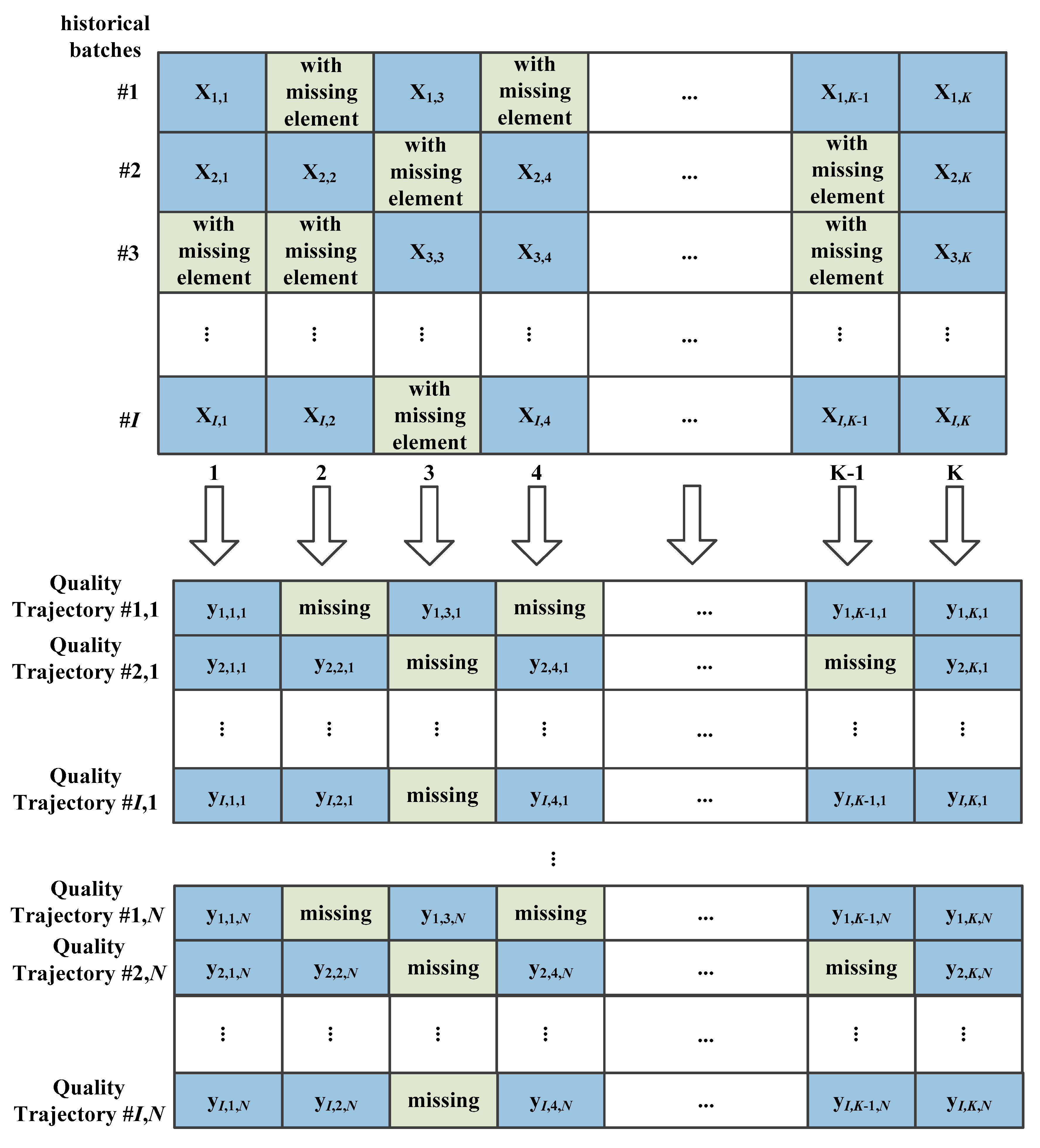
In the proposed method, bagging is introduced to generate output variables with different output modes. Bagging, also called bootstrap aggregating, was proposed by Leo Breiman to improve the performance of classification [33,34]. It is a machine-learning algorithm developed for ensemble learning to improve the performance in statistical classification and regression. It also improves reliability and reduces the chance of overfitting. For example, if historical batches of process variables have been obtained and N output modes exist, bagging is used to generate quality trajectories, which allows more batches than the original ones to be used to construct sub-models for further monitoring. The bagging strategy used for batch processes is shown in Figure 1, where quality trajectories are generated based on historical batches and output modes as a data re-sampling procedure.
According to the bagging strategy with the original process dataset , quality trajectories are established as , where represents batch numbers, represents the number of process variables, represents sample numbers in one batch and N is the number of output mode. Therefore, the re-sampled dataset for further training can be denoted as where . In the re-sampled dataset, reveals the total number of sub-dataset to construct individual sub-models for monitoring. In such a bagging approach, the new sub-datasets keep the complete information of the original dataset, including process dynamics for modeling, monitoring, and ensemble learning. However, it is noticed that the historical batches have missing values, which confront corresponding missing elements in quality trajectories and render further modeling and monitoring quite difficult.
3.2. Stochastic Programming for Quality-Relevant Monitoring
For each sub-dataset , it is necessary to construct a corresponding sub-model for quality-relevant monitoring. Based on the previous steps, the stochastic programming problem for quality-relevant monitoring of batch processes for each sub-model is formulated as follows (see also the standard formulation in Equation (1):
where is the optimal solution of the quality trajectory at time , , is the process output of batch calculated at time , hence represents the residual between the output and the optimal solution at time instant of the i-th batch; is the reconstructed value of that the m-th missing process variable of the i-th batch at time instant calculated on the basis of , is the m-th process variable of the i-th batch estimated by existing values of the corresponding variable at the same time; the weighting parameter during the optimization for quality residuals, and is the weighting parameter during the optimization for the reconstructed error for the m-th missing variable. Thus represents the error between the estimated and reconstructed value of the current process variable. For the vectors containing the elements and , respectively, is the system of equations that describe the constraints on the estimated process variables, while is the system of equations representing the constraints on the optimal quality variables.
In Equation (2), the stochastic programming problem can be solved by minimum search methods, since is the only unknown variable in this optimization problem. According to the relationship between the process variables and quality variables, the reconstructed value of process variable can be a function of the form , where . Therefore, the above problem becomes a multi-objective optimization problem at every time instant to find the optimal quality trajectory that minimizes the objective function.
Based on the solution to the above stochastic programming problem, N sub-models are constructed with the datasets , where and each sub-model has individual optimal solutions and corresponding residuals to implement subsequent monitoring steps in the proposed methodology.
3.3. Monitoring Statistics
For monitoring purposes, the average trajectory is usually calculated as the reference to determine the control limit based on (standard deviation) principle [35]. In each sub-model, the control limit of the traditional method at time instant is denoted as follows:
where is the upper control limit and is the lower control limit; represents the average trajectory and is the standard deviation of output trajectories at time instant .
In the proposed method, the datasets for modeling consist of different output modes, which means that the average trajectory is no longer a good reference for monitoring due to the variety of output trajectory and its non-Gaussian distribution. Besides, the problem of missing elements will influence the accuracy of calculation. To improve the reliability of the monitoring results, the optimal trajectory is regarded as the reference in each sub-model. Then the residuals from the optimal trajectory can be calculated to reveal whether the current output trajectory has a large deviation to the reference, which is even of great significance for further process optimization. The modified control limit in each sub-model is defined as follows:
where is the residual between the actual output and the optimal trajectory of the i-th batch at time instant , is the number of missing output elements at time instant and is the corresponding standard deviation of the residuals.
3.4. Bayesian Fusion Ensemble Strategy
Based on the current residuals in each sub-model as , these individual monitoring results are combined under Bayesian framework. In the proposed method, the Bayesian fusion (BF) strategy is used as the ensemble strategy for fault detection. The monitoring results are determined by the Bayesian rule as follows:
where represents the index of sub-models, “F” is fault condition and “N” is normal condition; , are the prior probabilities of the fault condition and normal condition, respectively. In such a strategy, can simply be regarded as the confidence level while can be determined as . Thus, to figure out the final fault probability given a new residual , and should be calculated at first. In the proposed method, they are determined as follows:
where is the upper control limit of sub-model as defined in Equation (6), is the average residual of sub-model calculated through the historical sub-dataset. Therefore, the corresponding fault probabilities have been obtained, where . Final decision should be made according to these individual monitoring results of different sub-models. Thus, the ensemble result is calculated as follows:
where denotes the probability that the current sample belongs to output mode . A simple case is that no prior knowledge can help to determine the probability of output modes, then is regarded as equal for each mode. Thus, Equation (12) can be simplified as follows:
Since the confidence level of the ensemble step is determined as , the process is judged to be abnormal if . On the contrary, the process is judged to be normal when .
3.5. Procedures and Discussions
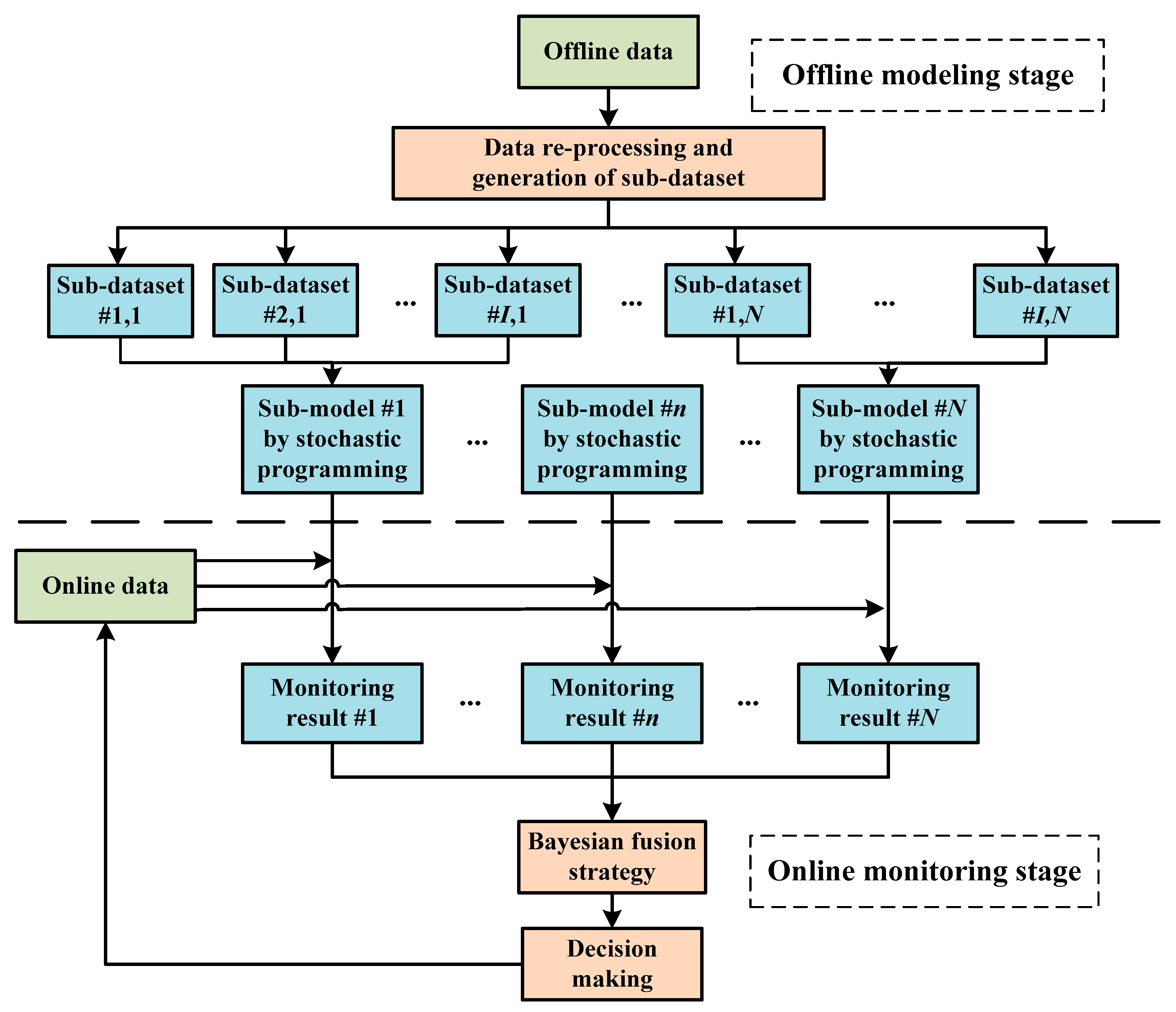
The main purpose of the methodology developed in this work is to achieve quality-relevant monitoring for batch processes based on stochastic programming and ensemble learning strategy. The implementation procedures are described as follows:
Step 1: Generate sub-datasets based on N output modes and historical dataset with batches process data.
Step 2: Calculate optimal quality trajectories for each sub-model by stochastic programming according to Equation (2).
Step 3: Construct N sub-models for monitoring purposes according to the residuals from optimal trajectories.
Step 4: Estimate quality trajectories of the current sample under different output modes.
Step 5: Introduce current quality trajectories to each sub-model and calculate residuals.
Step 6: Implement the Bayesian fusion strategy to combine the individual monitoring results.
The corresponding flow diagram of the proposed methodology is shown in Figure 2.
For most data-based monitoring methods, monitoring statistics are designed with control limits of different confidence levels. When the sample size is large enough and the distribution of samples can be identified, one reliable monitoring model is typically efficient for fault detection as it can adequately explain process conditions. However, when the sample size is small and the historical data is not enough (as is the case in the current work), it is difficult to construct an accurate monitoring model with limited data. Under such circumstances, errors will occur when process conditions experience significant variations since the limited data cannot adequately explain these complicated distributions again. For example, outliers may exist in historical data, and when the data sizes are not large enough to identify these outliers, the offline monitoring model will be affected. Meanwhile, the missing data problem will affect the modeling as well, especially for batch processes because of the batch-to-batch variations.
In the proposed method, stochastic programming is introduced to solve this problem by computing an optimal solution of historical quality trajectories, with the aid of partial knowledge related to process output, which accounts for intrinsic variabilities and uncertainties in the process and the quality data. To handle the problems of missing data and lack of historical batches, the bagging method is selected as a data re-sampling step to generate more sub-datasets with different output modes, which helps improve the robustness of offline modeling. As a result, an optimal quality-relevant trajectory obtained through stochastic programming is established. On the other hand, historical outputs can be compared with the optimal solution, generating residuals between them.
Generally, most data-based methods only have one monitoring model, and one implements a fault detection scheme merely based on the specific offline model. As described above, this may increase the chances of false or missed alarms due to the complex nature of process data in practical applications. Benefitting from the bagging method, several sub-models can be constructed and further used for ensemble learning. Hence, different sub-models have individual monitoring models with control limits according to the offline residuals.
For online monitoring purposes, the Bayesian fusion strategy is introduced for decision making as the ensemble learning method. Monitoring results of different individual sub-models are integrated under probabilistic framework, judging whether the current probability of abnormal condition at a specific time is more than the threshold that can be tolerated by the process.
In summary, the advantages of the proposed method include overcoming some of the limitations of traditional data-based monitoring methods, explicitly accounting for output uncertainties and variabilities, and making monitoring decisions in a robust ensemble learning way. Hence, compared to current data-based methods, both reliability and sensitivity are taken into consideration while implementing offline modeling and online monitoring.
4. Case Studies
Authors should discuss the results and how they can be interpreted in perspective of previous studies and of the working hypotheses. The findings and their implications should be discussed in the broadest context possible. Future research directions may also be highlighted.
In this section, two case studies are introduced to evaluate the performance of the proposed method. The first case study involves a numerical example, illustrating the monitoring results under different faulty conditions. The second case study is a fed-batch penicillin fermentation process, which is a benchmark process that is widely used in batch process simulations.
4.1. A Numerical Simulation
We consider a nonlinear system with 3 variables as follows:
where , , are the process variables, t represents the latent variable, , , are independent Gaussian noises, and , , represent model parameters in the equation between process variables and output variable. The above system is run for a finite time, and a total of 200 samples are generated in each batch. Several normal batches and two faulty batches are introduced to test the monitoring performance of the proposed method. To evaluate the performance under the conditions of missing and limited data, only 10 normal batches are generated as training data and 40 samples in each normal batch are randomly missing, which results in a complicated dataset for offline modeling. Therefore, the missing sample rate is 20%, and this system becomes a batch process example with limited historical batches and missing data.
The first fault considered is a gradual fault affecting variable 1, which is introduced from the 101st sample and returned to normal after the 150th sample. The system equations of process variables under this fault are given by:
The second fault is a step bias of variable 2, introduced between the 101st sample and the 150th sample. This step fault is described in process variables by:
Due to the limited batches and missing data of the historical dataset, the bagging method is used to generate 40 sub-datasets based on the original dataset and four output modes, preparing for the construction of 4 sub-models. In each sub-model, is extracted as process dataset and used as quality data. Since the stochastic nature of process output is taken into consideration, we assume that the parameters , , in Equation (14) vary from mode to mode as shown in Table 2. Hence, the optimal trajectories of the individual sub-models are computed using the proposed stochastic programming approach. All weighting parameters are set as 1 for simplicity.
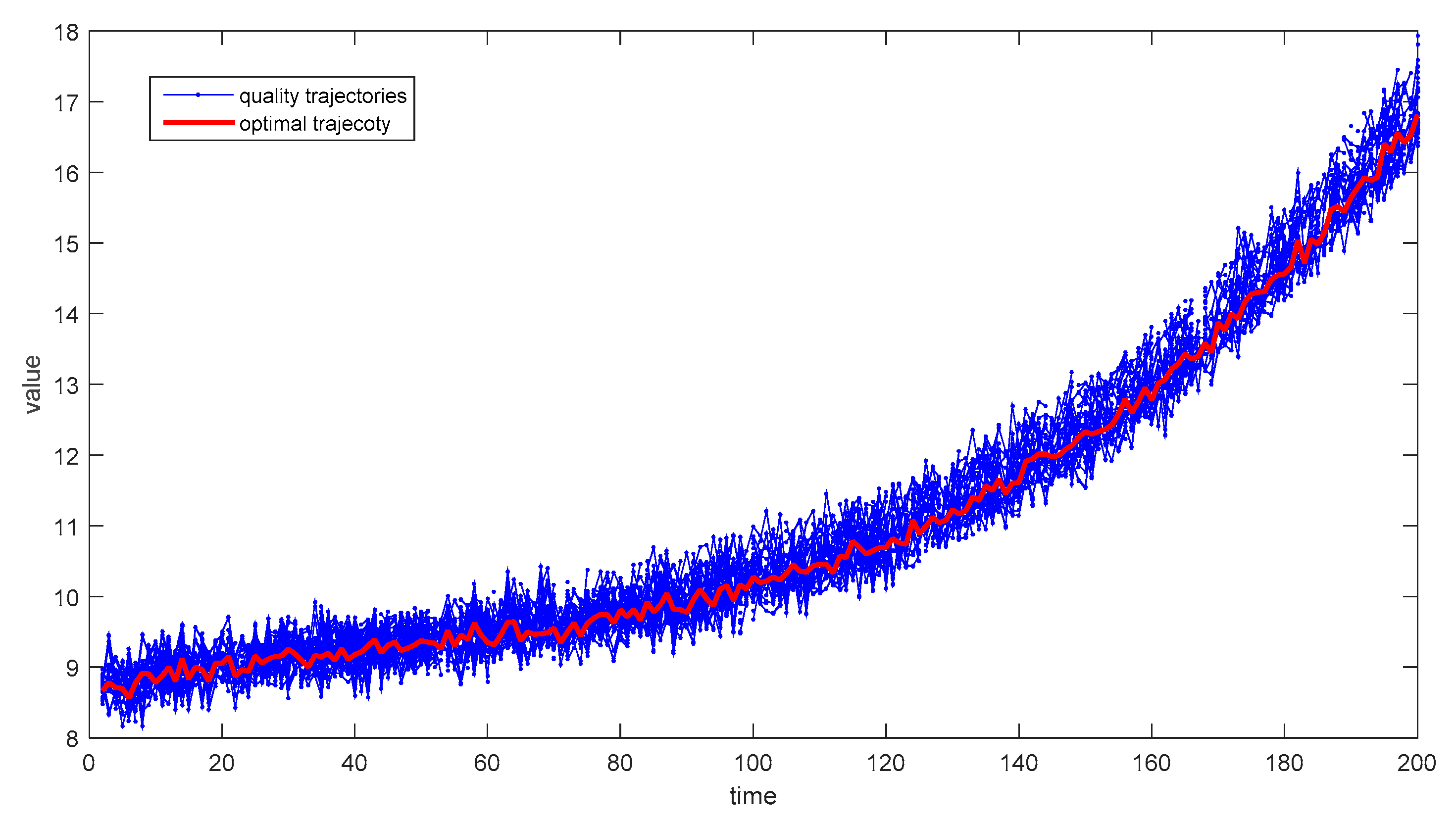
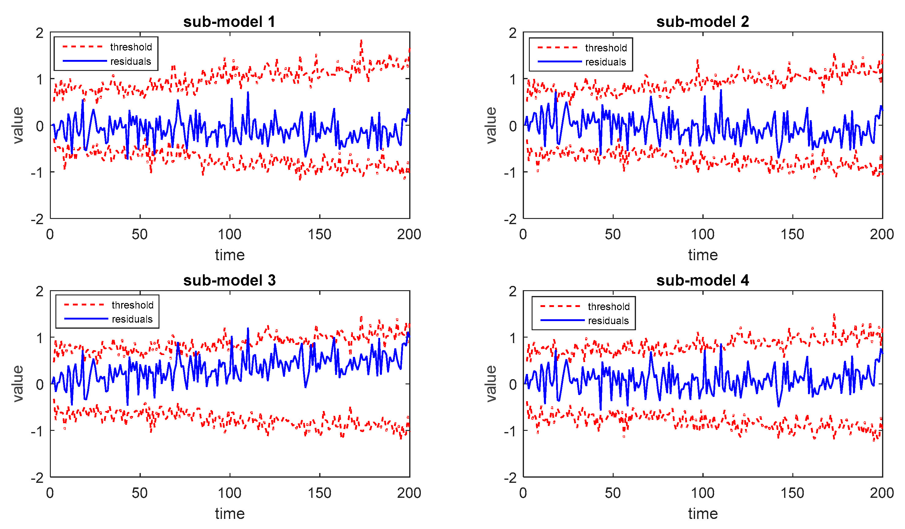
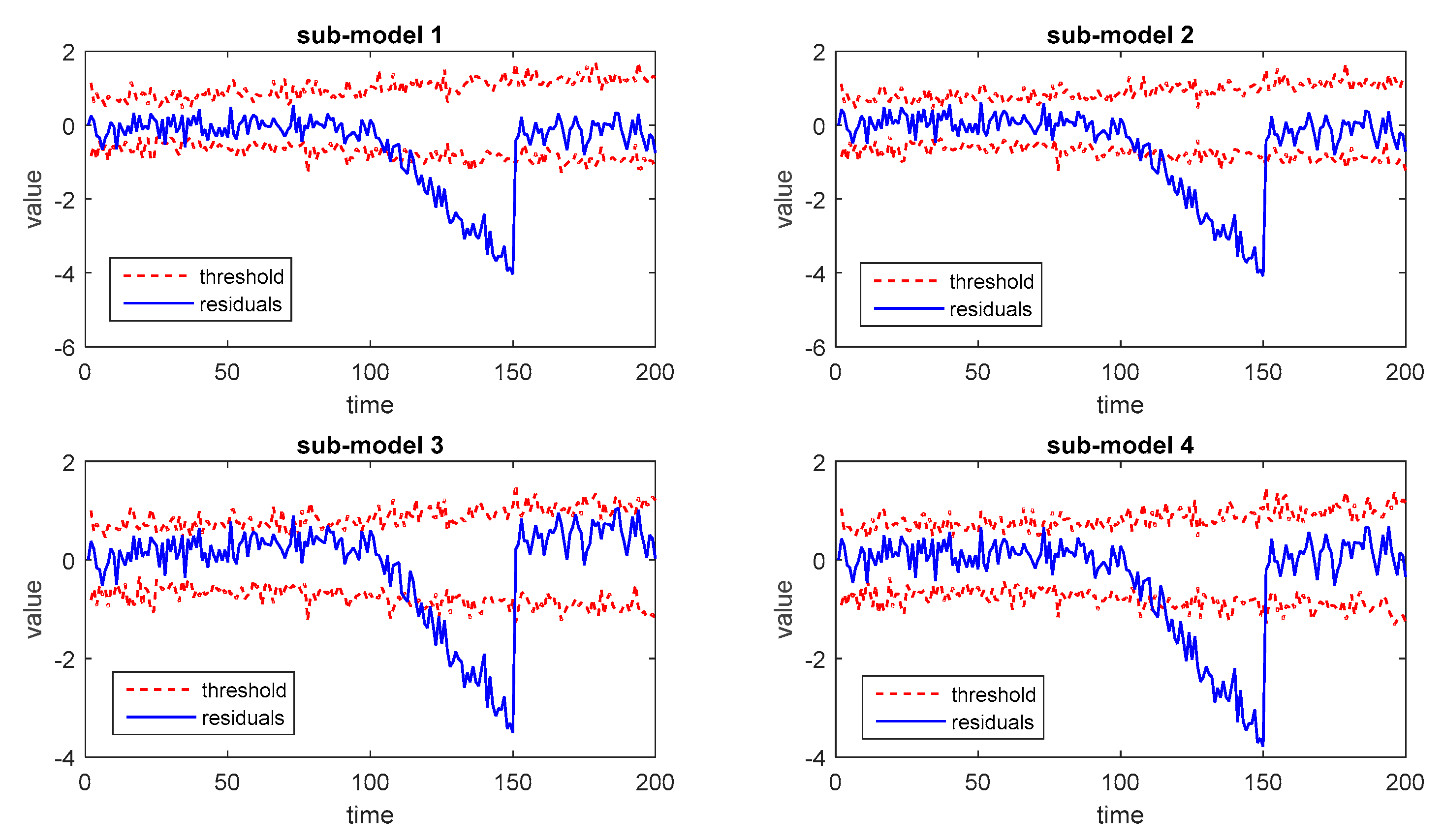
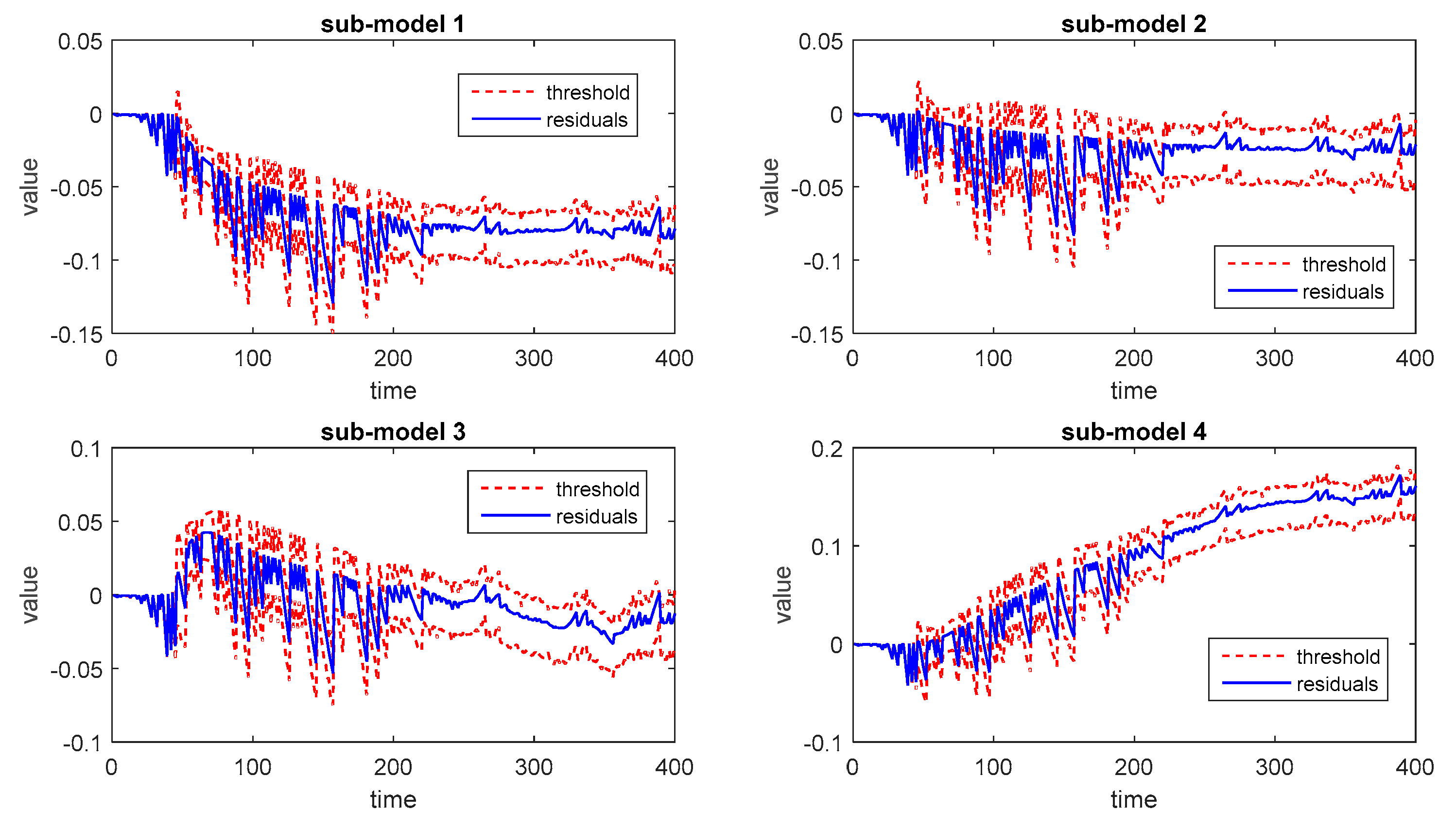
During the online monitoring procedures, one normal batch and two faulty batches are simulated to calculate the values of monitoring statistics at each time instant. After the implementation of stochastic programming with four modes, the optimal trajectory is calculated as shown in Figure 3. Then, the residuals between the optimal trajectories and the practical output are calculated to obtain monitoring statistics. Thus, the monitoring results of the normal batch for each sub-model are obtained and shown in Figure 4.
For the existing methods without the ensemble step, individual models are usually established to implement local monitoring tasks. When the ensemble strategy is introduced, the voting-based strategy is widely used to integrate the monitoring results of each individual model. Therefore, to demonstrate the advantages of the proposed method, comparisons of these conditions are considered in this case. The first contrast is implemented by using individual monitoring results of each sub-model directly without the ensemble learning strategy. Another one is executed by the use of a voting-based strategy as the ensemble step. These two comparisons are made to illustrate the advantages of the Bayesian fusion strategy based on stochastic programming.
In this case, the cutoff value of violation time for the voting-based strategy is set as 3, where most sub-models indicate abnormal conditions in such an ensemble strategy. As a result, the false alarm rate (FAR) of individual sub-models, voting-based strategy, and Bayesian fusion strategy can be calculated based on the testing normal batch.
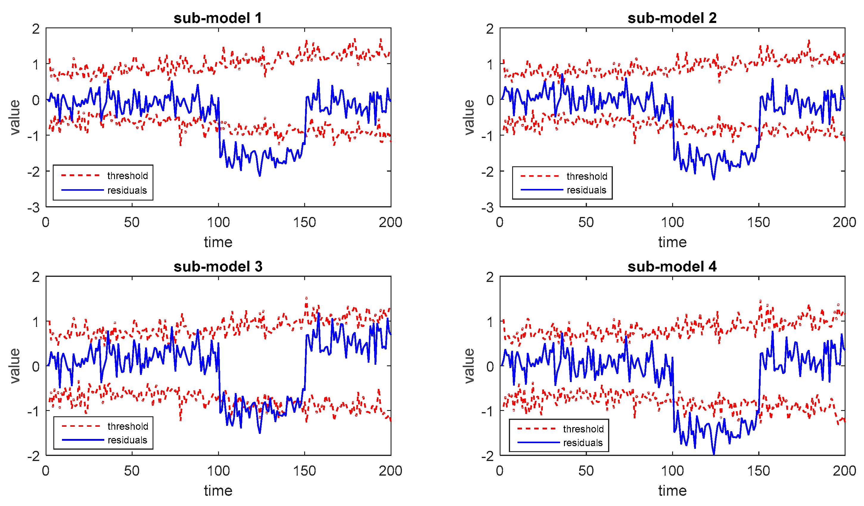
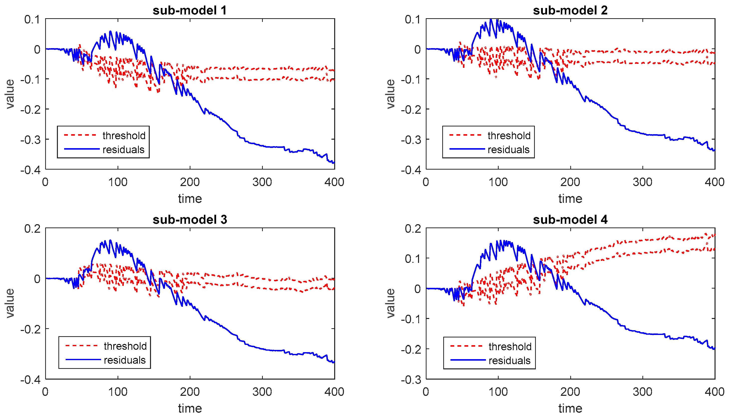
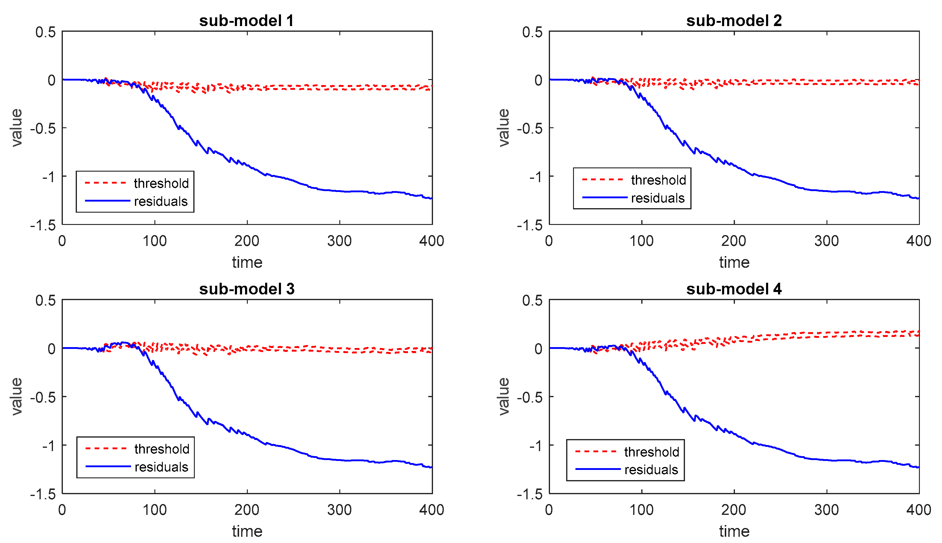
Next, the two abnormal batches are introduced as the testing faulty batches. The corresponding monitoring results of these two faulty batches based on different sub-models are shown in Figure 5 and Figure 6.
Therefore, false alarm rate (FAR) and fault detection rate (FDR) can be calculated according to different ensemble strategies. The overall monitoring results of the normal batch and two faulty batches are listed in Table 3.
It can be inferred that both results are acceptable due to the use of stochastic programming and the solution of optimal trajectory. Among these results, the results of individual sub-models are not reliable enough since the FDR varies from one sub-model to another and the FAR is much higher than the ensemble strategies. The FAR of voting-based strategy and Bayesian fusion strategy is close, while the FDR of BF is obviously higher than voting-based strategy. Besides, the monitoring results by using the average trajectory of different output modes are offered as well, which presents higher FAR and lower FDR with the same BF strategy.
According to the monitoring results of the numerical example, after the implementation of stochastic programming and the solution of the optimal quality trajectory, Bayesian fusion is a relatively better ensemble learning strategy to provide significant monitoring performance for batch processes with limited batches, missing elements, and multiple output modes.
4.2. Penicillin Fermentation Process
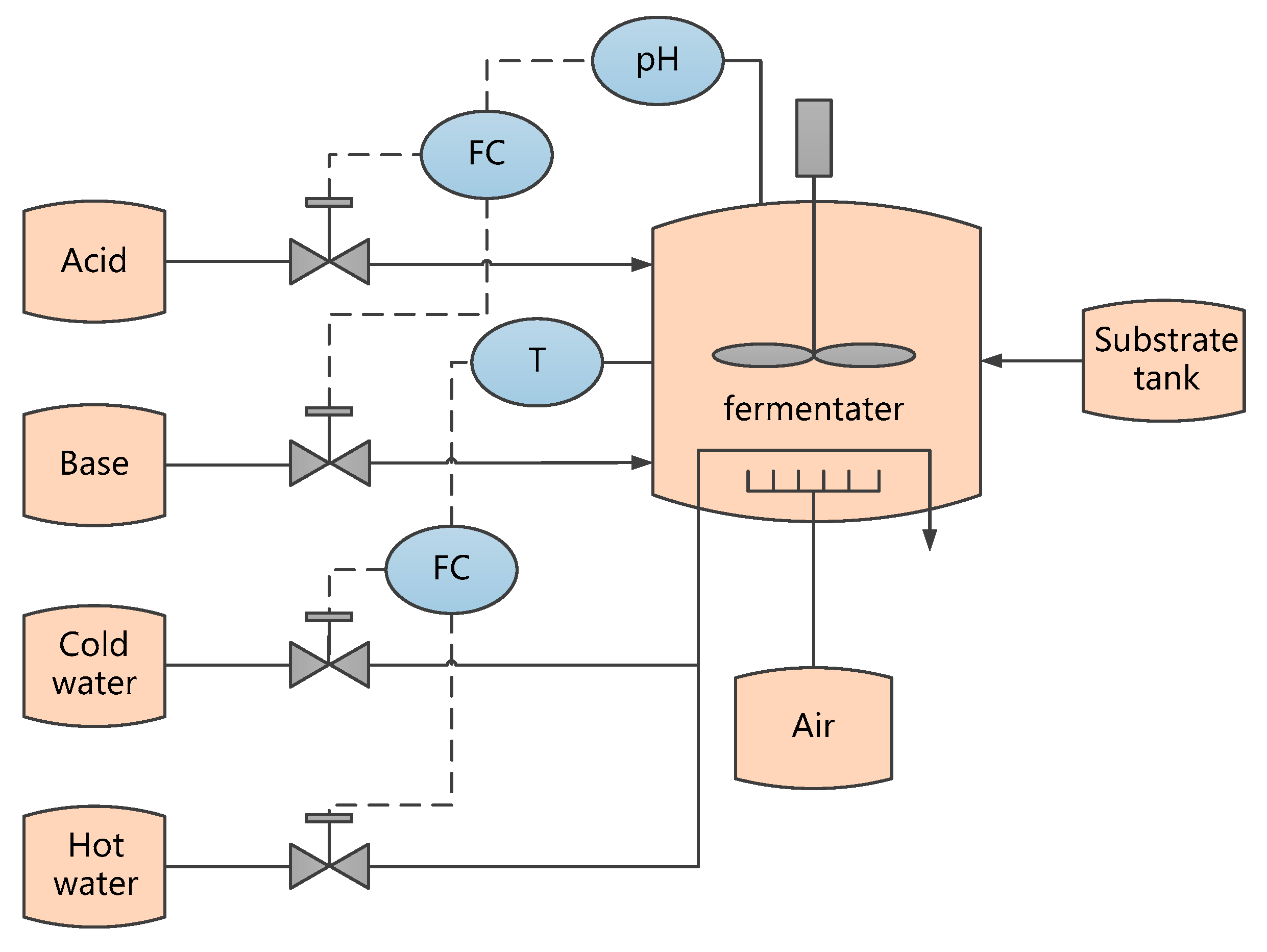
In this subsection, a simulation based on a fed-batch penicillin benchmark process is introduced to demonstrate the effectiveness of the proposed method. The benchmark software named PenSim v2.0 was developed by the Illinois Institute of Technology and can be found online [36]. The flowsheet of the penicillin process is shown in Figure 7. The process can be divided into two phases: a pre-culture phase for 40 hours for biomass growth, and a fed-batch phase for penicillin production. During the first stage, glucose is consumed and biomass grows for the preparation of penicillin production, followed by the second stage, where substrate is fed continuously and penicillin is produced until the end of the batch.
In this case study, 10 normal batches are generated by PenSim with 11 process variables, which are listed in Table 4. Similar to the numerical example presented in Section 4.1, the scale of historical data are small and insufficient. In each batch, 400 samples are generated and the sampling interval is set as one hour.
To estimate penicillin concentration for stochastic programming, the relationship between penicillin concentration and quality-relevant variables are calculated with different methods. The model equations used for calculation are given by:
where is penicillin concentration, is biomass concentration, is substrate concentration, is culture volume. The model parameters include , which is the penicillin hydrolysis rate constant, , which is the specific rate of penicillin production, , which is the inhibition constant, , which is the inhibition constant for product formation with the mean value, , which is the oxygen limitation constant, , which is the dissolved oxygen concentration, and , which is the exponent of .
As discussed in Section 2.1, these parameters are not pure constants, and some of them show stochastic variations under different conditions. The parameter estimation results can vary, depending on which identification method is used. For this case study, , , and are chosen as the stochastic parameters, since they may influence penicillin concentration more than other parameters. Hence, these model parameters are set to different values according to NPM, PSO, GSA and PenSim, respectively. The values of the parameters are listed in Table 5, which represents four output modes.
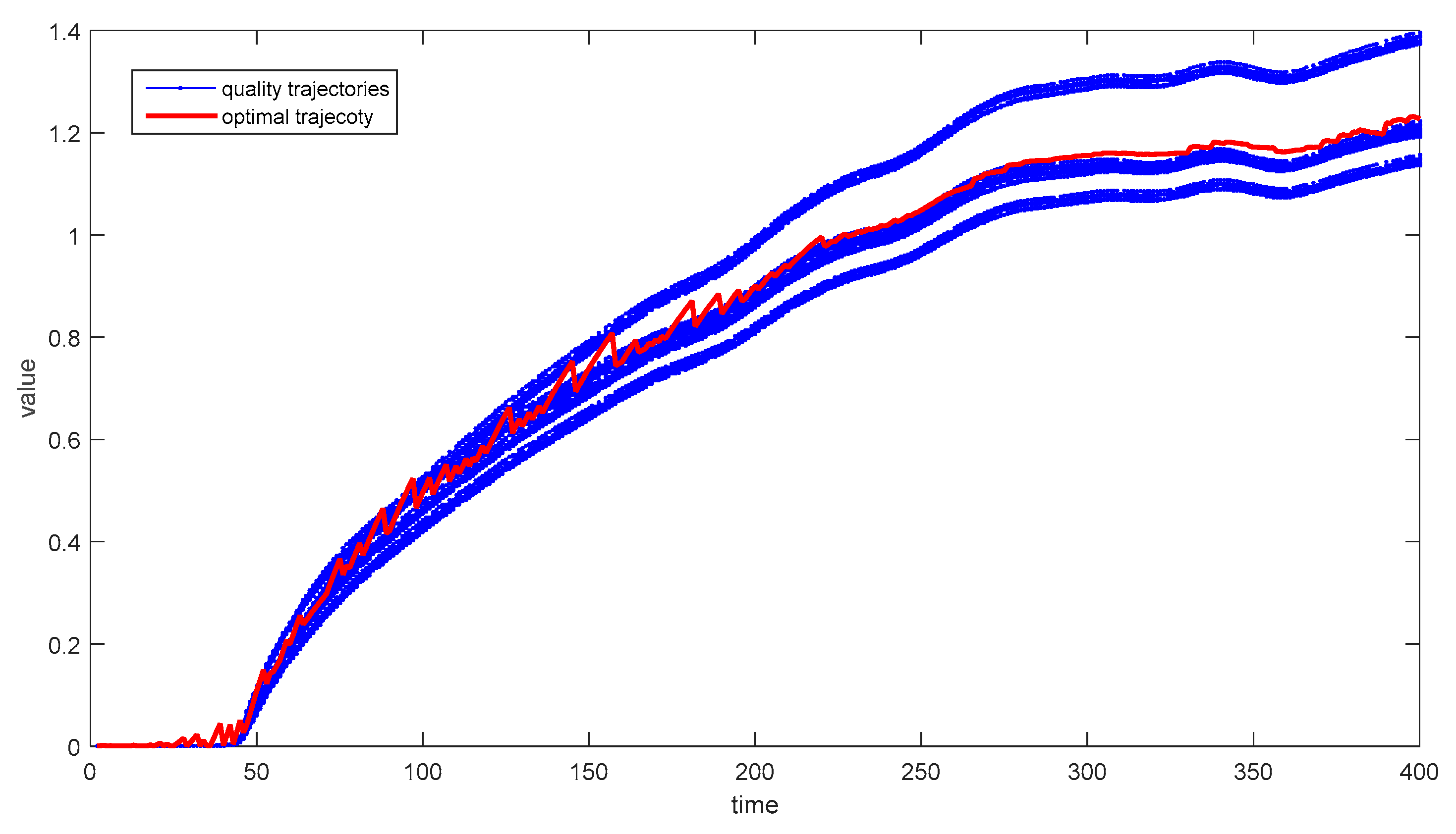
Similar to the numerical case presented earlier, all weight parameters are set as 1, and four sub-models are constructed based on stochastic programming for subsequent online monitoring. Although different output modes exist, constraints according to Equation (2) should be defined firstly, to make sure that the critical variables are varying within reasonable ranges. The corresponding constraints are listed in Table 6. Then, 40 random missing samples are considered in each historical batch data during the offline modeling step, and the corresponding missing sample rate for each batch is 10%. Thus, the optimal quality trajectory is calculated as shown in Figure 8.
Different from average trajectory, the optimal trajectory provides a better reference to process output with multiple output modes, limited batches, and missing elements in process data, which helps the construction of a more accurate monitoring model. Besides, the optimal solution has great significance for quality-relevant optimization and control of batch processes further.
For performance evaluation, one normal batch and three output-relevant faulty batches are generated as online data to test the performance of the proposed method. These faults are a step decrease of the substrate feed rate introduced from the 61st sample to the end of one batch as fault 1, a temperature controller failure from the beginning to the end as fault 2, and a pH controller failure from the beginning to the end as fault 3, respectively.
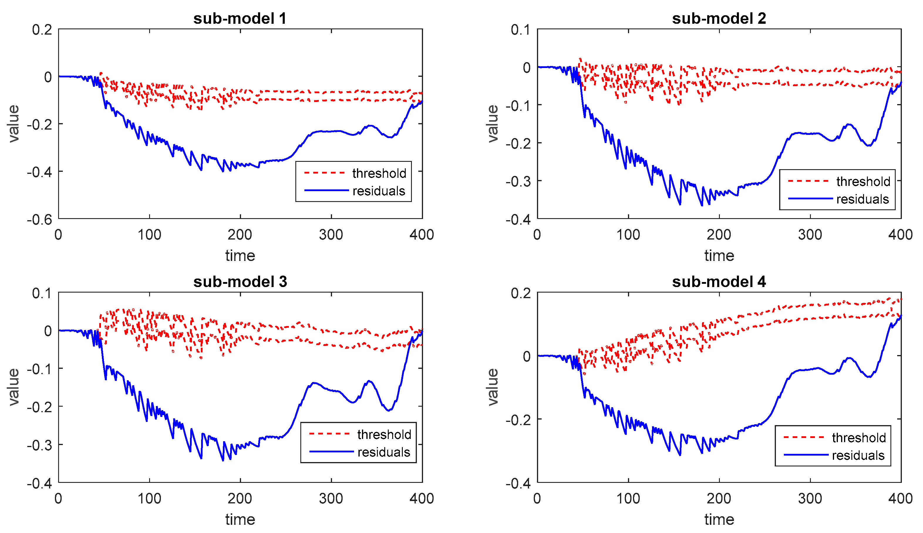
The monitoring results under normal conditions are shown in Figure 9. For the proposed method, the results are satisfactory and demonstrate that the process is operating under normal conditions during the run time. Furthermore, all sub-models provide consistently correct results since the control limits are tight and accurate.
Then the process monitoring results for fault 1, fault 2, and fault 3 are shown in Figure 10, Figure 11 and Figure 12, respectively. It can be seen that the proposed method is able to detect quality-relevant abnormal conditions after these faults occur.
The monitoring results of each sub-model are able to detect faults individually. However, the detailed monitoring performance varies from one sub-model to another. Similar to the first case, three kinds of decision-making strategies are implemented for performance evaluation. The corresponding FAR and FDR can be calculated according to each strategy and presented in Table 7. The FAR of fault 2 and fault 3 is not listed in the table because these faults occur at the beginning of one batch and exist throughout the process. Besides, the monitoring results by using the average trajectory of different output modes are provided as well with the similar BF ensemble strategy.
As illustrated in Table 7, no false alarm occurs for both methods under the framework of batch process monitoring based on stochastic programming. According to the comparison of FDR in faulty conditions, the BF strategy is proved to offer the most reliable monitoring performance among all of these decision-making strategies due to the highest overall FDR.
5. Discussions and Conclusions
In this paper, a robust monitoring method based on stochastic programming and ensemble learning was developed, to handle quality-relevant monitoring for batch processes with missing data and insufficient historical data. The focus of the developed method was on process quality, taking the stochastic nature of the process into account. For batch processes with multiple output modes and specific difficulties for monitoring listed above, the proposed method is able to deal with the problem effectively. However, for simple cases, where the batch trajectory is steady and without complicated process characteristics, the traditional methods may perform better compared to the proposed method with less computation load.
The effectiveness of the proposed method was demonstrated in two case studies. Future work will focus on the application of the proposed method on a practical case, which is an aluminum foil annealing batch process.
Author Contributions
Conceptualization, methodology, F.S.; validation, J.Z.; writing—review and editing, F.S.; project administration, L.Y.; funding acquisition, D.G. All authors have read and agree to the published version of the manuscript.
Funding
This research was funded by the National Natural Science Foundation of China, grant number 61673349, the Natural Science Foundation of Zhejiang, grant number LQ19F030004, the General Scientific Research Project of Zhejiang Department of Education, grant number Y201839765, and the Foundation of Key Laboratory of Advanced Process Control for Light Industry (Jiangnan University), grant number APCLI1804.
Conflicts of Interest
The authors declare no conflict of interest.
References
- Li, D.; He, S.; Xi, Y.; Liu, T.; Gao, F.; Lu, J. Synthesis of ILC-MPC controller with data-driven approach for constrained batch processes. IEEE Trans. Ind. Electron. 2019, 67, 3116–3125. [Google Scholar] [CrossRef]
- Onel, M.; Kieslich, C.A.; Guzman, Y.A.; Floudas, C.A.; Pistikopoulos, E.N. Big Data Approach to Batch Process Monitoring: Simultaneous Fault Detection and Diagnosis Using Nonlinear Support Vector Machine-based Feature Selection. Comput. Chem. Eng. 2018, 115, 46–63. [Google Scholar] [CrossRef]
- Ye, L.; Guan, H.; Yuan, X.; Ma, X. Run-to-run optimization of batch processes with self-optimizing control strategy. Can. J. Chem. Eng. 2017, 95, 724–736. [Google Scholar] [CrossRef]
- Zhou, L.; Chen, J.; Song, Z. Recursive Gaussian process regression model for adaptive quality monitoring in batch processes. Math. Probl. Eng. 2015, 2015, 1–9. [Google Scholar] [CrossRef]
- Qin, S.J.; Zheng, Y. Quality-relevant and process-relevant fault monitoring with concurrent projection to latent structures. Aiche J. 2013, 59, 496–504. [Google Scholar] [CrossRef]
- Chu, F.; Cheng, X.; Jia, R.; Wang, F.; Lei, M. Final quality prediction method for new batch processes based on improved JYKPLS process transfer model. Chemometr. Intell. Lab. Syst. 2018, 183, 1–10. [Google Scholar] [CrossRef]
- Peng, K.; Li, Q.; Zhang, K.; Dong, J. Quality-related process monitoring for dynamic non-Gaussian batch process with multi-phase using a new data-driven method. Neurocomputing 2016, 214, 317–328. [Google Scholar] [CrossRef]
- Wang, X.; Wang, P.; Gao, X.; Qi, Y. On-line quality prediction of batch processes using a new kernel multiway partial least squares method. Chemometr. Intell. Lab. Syst. 2016, 158, 138–145. [Google Scholar] [CrossRef]
- Mori, J.; Yu, J. Quality relevant nonlinear batch process performance monitoring using a kernel based multiway non-Gaussian latent subspace projection approach. J. Process Control 2014, 24, 57–71. [Google Scholar] [CrossRef]
- Shen, F.; Ge, Z.; Song, Z. Multivariate trajectory-based local monitoring method for multiphase batch processes. Ind. Eng. Chem. Res. 2015, 54, 1313–1325. [Google Scholar] [CrossRef]
- He, Y.; Zhou, L.; Ge, Z.; Song, Z. Dynamic Mutual Information Similarity Based Transient Process Identification and Fault Detection. Can. J. Chem. Eng. 2018, 96, 1541–1558. [Google Scholar] [CrossRef]
- Zhou, L.; Chen, J.; Song, Z.; Ge, Z. Semi-supervised PLVR models for process monitoring with unequal sample sizes of process variables and quality variables. J. Process Control 2015, 26, 1–16. [Google Scholar] [CrossRef]
- Zhou, L.; Chen, J.; Song, Z.; Ge, Z.; Miao, A. Probabilistic latent variable regression model for process-quality monitoring. Chem. Eng. Sci. 2014, 116, 296–305. [Google Scholar] [CrossRef]
- Lopez-Montero, E.B.; Wan, J.; Marjanovic, O. Trajectory tracking of batch product quality using intermittent measurements and moving window estimation. J. Process Control 2015, 25, 115–128. [Google Scholar] [CrossRef] [Green Version]
- Yuan, X.; Wang, Y.; Yang, C.; Ge, Z.; Song, Z.; Gui, W. Weighted linear dynamic system for feature representation and soft sensor application in nonlinear dynamic industrial processes. IEEE Trans. Ind. Electron. 2017, 65, 1508–1517. [Google Scholar] [CrossRef]
- Arteaga, F.; Ferrer, A. Dealing with missing data in MSPC: Several methods, different interpretations, some examples. J. Chemometr. 2002, 16, 408–418. [Google Scholar] [CrossRef]
- Stanimirova, I.; Daszykowski, M.; Walczak, B. Dealing with missing values and outliers in principal component analysis. Talanta 2007, 72, 172–178. [Google Scholar] [CrossRef]
- Nelson, P.R.C.; Taylor, P.A.; MacGregor, J.F. Missing data methods in PCA and PLS: Score calculations with incomplete observations. Chemom. Intell. Lab. Syst. 1996, 35, 45–65. [Google Scholar] [CrossRef]
- Soares, E.; Costa, P.; Costa, B.; Leite, D. Ensemble of Evolving Data Clouds and Fuzzy Models for Weather Time Series Prediction. Appl. Soft Comput. 2018, 64, 445–453. [Google Scholar] [CrossRef]
- Jiang, Q.; Yan, X.; Huang, B. Review and Perspectives of Data-Driven Distributed Monitoring for Industrial Plant-Wide Processes. Ind. Eng. Chem. Res. 2019, 58, 12899–12912. [Google Scholar] [CrossRef]
- Kourti, T.; Nomikos, P.; MacGregor, J.F. Analysis, monitoring and fault diagnosis of batch processes using multiblock and multiway PLS. J. Process Control 1995, 5, 277–284. [Google Scholar] [CrossRef]
- Tong, C.; El-Farra, N.H.; Palazoglu, A.; Yan, X. Fault detection and isolation in hybrid process systems using a combined data-driven and observer-design methodology. Aiche J. 2014, 60, 2805–2814. [Google Scholar] [CrossRef]
- Ge, Z. Review on data-driven modeling and monitoring for plant-wide industrial processes. Chemom. Intell. Lab. Syst. 2017, 171, 16–25. [Google Scholar] [CrossRef]
- Birge, J.R.; Louveaux, F. Introduction to Stochastic Programming, 2nd ed.; Springer: New York, NY, USA, 2011; pp. 1–19. [Google Scholar]
- Wang, L.; Chen, J.; Pan, F. Applications of gravitational search algorithm in parameters estimation of penicillin fermentation process model. J. Comput. Appl. 2013, 33, 3296–3299. [Google Scholar] [CrossRef]
- Eronen, V.P.; Kronqvist, J.; Westerlund, T.; Mäkelä, M.M.; Karmitsa, N. Method for solving generalized convex nonsmooth mixed-integer nonlinear programming problems. J. Global. Optim. 2017, 69, 443–459. [Google Scholar] [CrossRef]
- Gong, Y.J.; Li, J.J.; Zhou, Y.; Li, Y.; Chung, H.S.H.; Shi, Y.H.; Zhang, J. Genetic Learning Particle Swarm Optimization. IEEE Trans.Cybern. 2016, 46, 2277–2290. [Google Scholar] [CrossRef] [Green Version]
- Cuevas, E.; Díaz, P.; Avalos, O.; Zaldívar, D.; Pérez-Cisneros, M. Nonlinear system identification based on ANFIS-Hammerstein model using Gravitational search algorithm. Appl. Intell. 2018, 48, 182–203. [Google Scholar] [CrossRef]
- Dantzig, G.B.; Infanger, G. Multi-stage stochastic linear programs for portfolio optimization. Ann. Oper. Res. 1993, 45, 59–76. [Google Scholar] [CrossRef] [Green Version]
- Beraldi, P.; Bruni, M.E.; Manerba, D.; Mansini, R. A Stochastic Programming Approach for the Traveling Purchaser Problem. IMA J. Manage. Math. 2017, 28, 41–63. [Google Scholar] [CrossRef]
- Ge, Z.; Huang, B.; Song, Z. Mixture semisupervised principal component regression model and soft sensor application. AIChE J. 2014, 60, 533–545. [Google Scholar] [CrossRef]
- Yuan, X.; Ge, Z.; Song, Z. Soft sensor model development in multiphase/multimode processes based on Gaussian mixture regression. Chemometr. Intell. Lab. Syst. 2014, 138, 97–109. [Google Scholar] [CrossRef]
- Breiman, L. Bagging Predictors. Mach. Learn. 1996, 24, 123–140. [Google Scholar] [CrossRef] [Green Version]
- Ge, Z.; Song, Z. Bagging support vector data description model for batch process monitoring. J. Process Control 2013, 23, 1090–1096. [Google Scholar] [CrossRef]
- Cimander, C.; Mandenius, C.F. Bioprocess control from a multivariate process trajectory. Bioprocess. Biosyst. Eng. 2004, 26, 401–411. [Google Scholar] [CrossRef]
- Birol, G.; Ündey, C.; Çinar, A. A modular simulation package for fed-batch fermentation: Penicillin production. Comput. Chem. Eng. 2002, 26, 1553–1565. [Google Scholar] [CrossRef]
Figure 1.
Bagging for batch processes with I batches and N output modes.

Figure 2.
Flow diagram of the proposed methodology.

Figure 3.
The solution of optimal trajectory in numerical example.

Figure 4.
Monitoring results of the normal batch in numerical example.

Figure 5.
Monitoring results of fault 1 in numerical example.

Figure 6.
Monitoring results of fault 2 in numerical example.

Figure 7.
Flow diagram of penicillin fermentation process.

Figure 8.
The solution of optimal trajectory in penicillin fermentation case.

Figure 9.
Monitoring results of the normal batch in penicillin fermentation case.

Figure 10.
Monitoring results of fault 1 in penicillin fermentation case.

Figure 11.
Monitoring results of fault 2 in penicillin fermentation case.

Figure 12.
Monitoring results of fault 3 in penicillin fermentation case.


Table 1.
Comparison of parameter estimation results for different methods.
| Parameter | Result | NPM | PSO | GSA |
|---|---|---|---|---|
| μx | Mean value | 0.0913 | 0.0964 | 0.0997 |
| Standard deviation | 0.0002 | 0.0007 | 0.0004 | |
| Kx | Mean value | 0.1362 | 0.1484 | 0.1512 |
| Standard deviation | 0.0016 | 0.0285 | 0.0030 | |
| KI | Mean value | 0.0402 | 0.1441 | 0.1090 |
| Standard deviation | 0.0012 | 0.0093 | 0.0151 | |
| K | Mean value | 0.0016 | 0.0445 | 0.0599 |
| Standard deviation | 0.0155 | 0.0103 | ||
| μp | Mean value | 0.0033 | 0.0048 | 0.0064 |
| Standard deviation | 0.0014 | 0.0009 | ||
| Yx/s | Mean value | 0.2860 | 0.4228 | 0.4441 |
| Standard deviation | 0.0021 | 0.0229 | 0.0175 | |
| ms | Mean value | 0.0040 | 0.0137 | 0.0136 |
| Standard deviation | 0.0002 | 0.0012 | 0.0013 |
Table 2.
Parameter values of different output modes in numerical example.
| a | b | c | |
|---|---|---|---|
| Mode 1 | 5.00 | −0.5 | 1.52 |
| Mode 2 | 5.06 | −0.53 | 1.58 |
| Mode 3 | 4.95 | −0.50 | 1.60 |
| Mode 4 | 5.12 | −0.47 | 1.50 |
Table 3.
FAR and FDR under different ensemble strategies in numerical example.
| Batch Type | Result | Sub-Model 1 | Sub-Model 2 | Sub-Model 3 | Sub-Model 4 | Voting-Based Strategy | BF with Optimal Trajectory | BF with Average Trajectory |
|---|---|---|---|---|---|---|---|---|
| Normal | FAR | 0.020 | 0.015 | 0.030 | 0.005 | 0.005 | 0.005 | 0.007 |
| Fault 1 | FDR | 0.800 | 0.800 | 0.680 | 0.740 | 0.740 | 0.800 | 0.720 |
| FAR | 0.020 | 0.013 | 0.033 | 0.007 | 0.007 | 0.007 | 0.013 | |
| Fault 2 | FDR | 1.000 | 1.000 | 0.720 | 0.980 | 0.980 | 1.000 | 0.960 |
| FAR | 0.007 | 0.013 | 0.033 | 0.007 | 0.007 | 0.007 | 0.020 |
Table 4.
Variables selected for monitoring in penicillin fermentation case.
| Number | Variables |
|---|---|
| 1 | Aeration rate (l/h) |
| 2 | Agitator power (W) |
| 3 | Substrate feed rate (l/h) |
| 4 | Substrate feed temperature (K) |
| 5 | pH |
| 6 | Generated heat (kcal) |
| 7 | Substrate concentration (g/L) |
| 8 | Dissolved oxygen concentration (g/L) |
| 9 | Biomass concentration (g/L) |
| 10 | Culture volume (L) |
| 11 | Carbon dioxide concentration (g/L) |
Table 5.
Values of model parameters in penicillin fermentation case.
| Parameter | NPM | PSO | GSA | PenSim |
|---|---|---|---|---|
| μp | 0.0043 | 0.0048 | 0.0064 | 0.0050 |
| Kp | 0.0002 | 0.0002 | 0.0002 | 0.0002 |
| KI | 0.1002 | 0.1041 | 0.1090 | 0.1000 |
| K | 0.0416 | 0.0445 | 0.0599 | 0.0400 |
Table 6.
Constraints of the critical variables.
| Variables | Constraints |
|---|---|
| Aeration rate (x1) | 8.5 L/h < x1 < 8.7 L/h |
| Agitator power (x2) | 29 W < x2 < 31 W |
| Substrate feed temperature (x3) | 295 K < x3 < 300 K |
| pH (x4) | 4.7 < x4 < 5.5 |
| Culture volume (x5) | 95 L < x5 < 110 L |
| Penicillin concentration (y) | 0 < y < 1.5 g/L |
Table 7.
FAR and FDR under different ensemble strategies in penicillin fermentation case.
| Batch Type | Result | Sub-Model 1 | Sub-Model 2 | Sub-Model 3 | Sub-Model 4 | Voting-Based Strategy | BF with Optimal Trajectory | BF with Average Trajectory |
|---|---|---|---|---|---|---|---|---|
| Normal | FAR | 0 | 0 | 0 | 0 | 0 | 0 | 0 |
| Fault 1 | FDR | 0.9353 | 0.9382 | 0.9441 | 0.9353 | 0.9265 | 0.9441 | 0.9323 |
| FAR | 0 | 0 | 0 | 0 | 0 | 0 | 0 | |
| Fault 2 | FDR | 0.8250 | 0.8250 | 0.8350 | 0.8250 | 0.8250 | 0.8275 | 0.8225 |
| Fault 3 | FDR | 0.9225 | 0.9150 | 0.8900 | 0.9225 | 0.9150 | 0.9200 | 0.9000 |
© 2020 by the authors. Licensee MDPI, Basel, Switzerland. This article is an open access article distributed under the terms and conditions of the Creative Commons Attribution (CC BY) license (http://creativecommons.org/licenses/by/4.0/).
Share and Cite
MDPI and ACS Style
Shen, F.; Zheng, J.; Ye, L.; Gu, D. Quality-Relevant Monitoring of Batch Processes Based on Stochastic Programming with Multiple Output Modes. Processes 2020, 8, 164. https://0-doi-org.brum.beds.ac.uk/10.3390/pr8020164
AMA Style
Shen F, Zheng J, Ye L, Gu D. Quality-Relevant Monitoring of Batch Processes Based on Stochastic Programming with Multiple Output Modes. Processes. 2020; 8(2):164. https://0-doi-org.brum.beds.ac.uk/10.3390/pr8020164
Chicago/Turabian StyleShen, Feifan, Jiaqi Zheng, Lingjian Ye, and De Gu. 2020. "Quality-Relevant Monitoring of Batch Processes Based on Stochastic Programming with Multiple Output Modes" Processes 8, no. 2: 164. https://0-doi-org.brum.beds.ac.uk/10.3390/pr8020164
Note that from the first issue of 2016, this journal uses article numbers instead of page numbers. See further details here.