Dynamic Optimization of a Fed-Batch Nosiheptide Reactor

Abstract

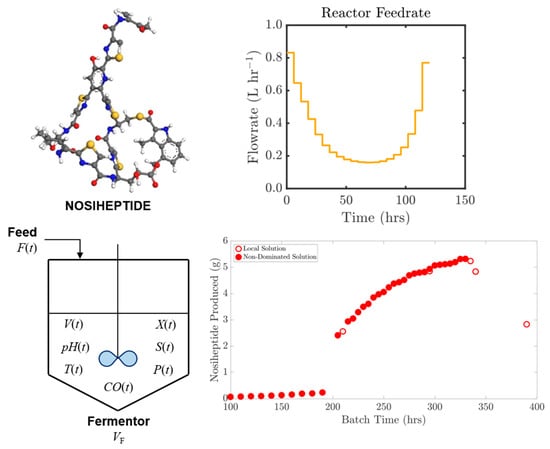
Nosiheptide is a sulfur-containing peptide antibiotic, showing exceptional activity against critical pathogens such as methicillin-resistant Staphylococcus aureus (MRSA) and vancomycin-resistant Enterococci (VRE) with livestock applications that can be synthesized via fed-batch fermentation. A simplified mechanistic fed-batch fermentation model for nosiheptide production considers temperature- and pH-dependence of biomass growth, substrate consumption, nosiheptide production and oxygen mass transfer into the broth. Herein, we perform dynamic simulation over a broad range of possible feeding policies to understand and visualize the region of attainable reactor performances. We then formulate a dynamic optimization problem for maximization of nosiheptide production for different constraints of batch duration and operability limits. A direct method for dynamic optimization (simultaneous strategy) is performed in each case to compute the optimal control trajectories. Orthogonal polynomials on finite elements are used to approximate the control and state trajectories allowing the continuous problem to be converted to a nonlinear program (NLP). The resultant large-scale NLP is solved using IPOPT. Optimal operation requires feedrate to be manipulated in such a way that the inhibitory mechanism of the substrate can be avoided, with significant nosiheptide yield improvement realized.

1. Introduction

1.1. Nosiheptide

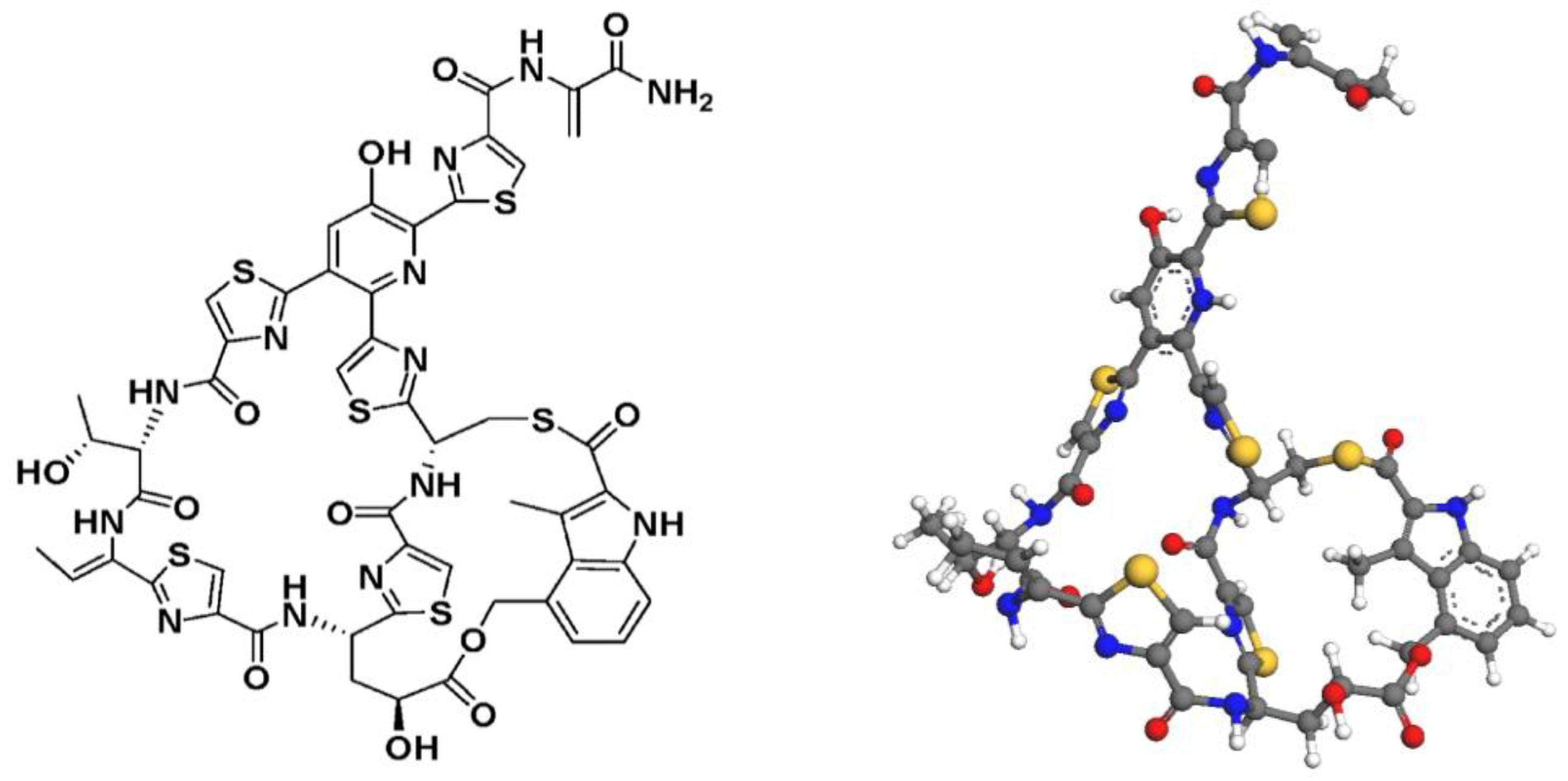
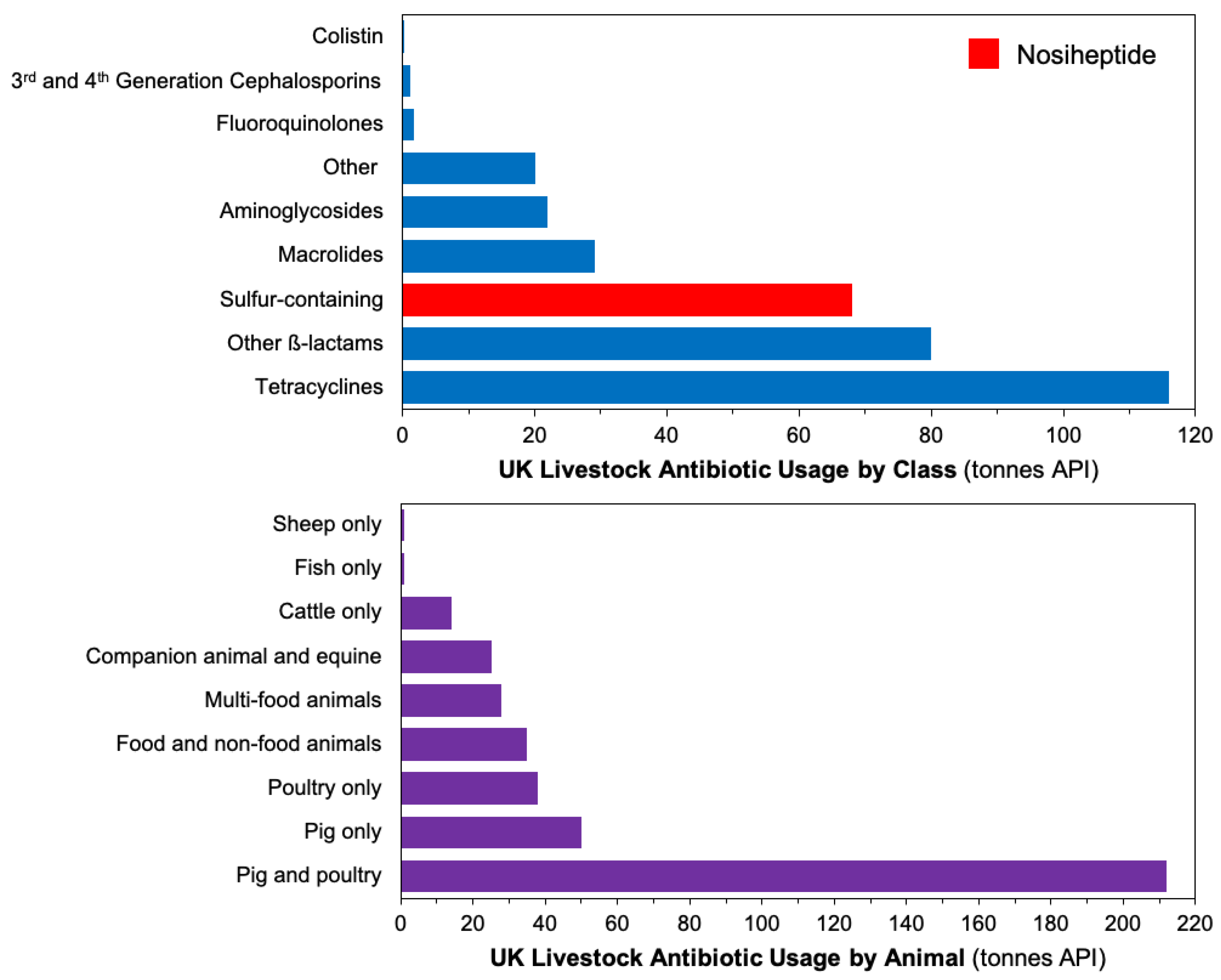
Antibiotics are essential pharmaceutical products in modern society [1], whose syntheses either require complex multistep chemical routes [2,3] or make use of enzymatic pathways [4] to obtain their complex molecular structures. Designing efficient antibiotic manufacturing processes is imperative. Nosiheptide (Figure 1) is a sulfur-containing peptide antibiotic obtained through fermentation. It exerts exceptional antibiotic activity in vitro and in a mouse model against critical Gram-positive pathogens such as methicillin-resistant Staphylococcus aureus (MRSA), vancomycin-resistant Enterococci (VRE) or Clostridium difficile. Nosiheptide and other thiopeptides’ mechanisms of action are a result of binding on the 50S ribosomal subunit which prevents selective protein synthesis. Shown non-toxic at high dosages, nosiheptide is principally used for livestock applications [5]. Figure 2 shows sales volumes of different antibiotic classes for livestock, with sulfur-containing antibiotics (including nosiheptide) being one of the top sellers. Recently the first total synthesis of nosiheptide was reported, utilizing double macro-cyclization of a fully-functionalized linear precursor [6]. Given low industrial yields, strong motivation exists to dynamically-optimize the process for improved product yield while reducing production time and cost to improve the industrial relevancy of manufacturing this antibiotic [7,8].

1.2. Process Modeling and Optimization Studies

Antibiotics are often produced via batch or fed-batch bioprocessing and frequently using enzymatic pathways. Dynamic modeling, simulation, and optimization are used for theoretical understanding of complex reaction networks inherent of biopharmaceutical production and to elucidate optimal control trajectories/operating policies to meet specific targets (e.g., maximize yield subject to purity constraints) [10]. Human antibiotic production, particularly β-lactams (whose broad applications and importance in global healthcare make them high priority), has received a lot of attention in process systems engineering in the past decade; a summary of pertinent literature examples on modeling and optimization of antibiotic production is provided in

Table 1. Select modeling and optimization studies for human β-lactam antibiotic production.

Antibiotic	Application	Study	Reference
Amoxicillin	Tonsillitis Bronchitis Pneumonia Gonorrhea Sinus infections UTIs	Application of artificial neural networks (ANNs) to model complex reaction scheme for penicillin G acylase (PGA)-catalyzed synthesis	[12]
		Inclusion of additional experimental data to improve ANN in reference [12]	[13]
		Maximization of API formation vs. different operating conditions in either methanol/ethylene glycol as reaction solvents	[14]
		Sensitivity analysis on previous ANN study [12]	[15]
		Modeling and simulation of continuous reactive crystallization in presence of substrates and impurities	[16,17]
		Dynamic optimization of non-isothermal batch reactor	[18]
Ampicillin	UTIs Pneumonia Gonorrhea Meningitis Abdominal infections	Regression of nucleation and growth kinetics for pH crystallization model	[19]
		Modeling and simulation of reactive crystallization in presence of substrates and impurities	[20]
		Modeling and simulation of continuous reactive crystallization in presence of substrates and impurities	[16,17]
		Multi-objective dynamic optimization of pH crystallization	[21]
Cephalexin	UTIs Respiratory tract infections Ear infections Skin infections	Non-isothermal modeling of enzymatic cephalexin batch synthesis	[22]
		Optimization of synthesis pH, temperature, and concentrations	[23]
		Non-isothermal modeling of enzymatic cephalexin batch synthesis	[24]
		Modeling and simulation of reactive crystallization in presence of substrates and impurities	[16,17]
		Regression of nucleation and growth kinetics for pH crystallization model	[25]

.

Modeling and optimization of fed-batch biopharmaceutical processes have also received significant attention for a wide variety of products, literature examples of which are summarized in

Table 2. Select modeling and optimization studies for fed-batch pharmaceutical production.

	Product		Biomass	Substrate	Objectives	Observations	Reference
	Molecule	Application
1	Podophyllotoxin	Anticancer	Podophyllum hexandrum	Indoleacetic acid, glucose, oxygen	Regress model parameters from batch data to inform fed-batch design	Increased volumetric productivity by 35.8%.	[26]
2	Unnamed protein	Unknown	Unnamed	Glucose, oxygen	Application of ANNs to model bioprocess	ANN formulated to capture industrial process behavior.	[27]
3	Fluoroleucine ethyl ester	Pharmaceutical intermediate	Candida antarctica	Azlactone, ethanol	Kinetic parameter regression for fed-batch process optimization	400% increase in fed-batch mode productivity vs. batch operation	[28]
4	Glutamine	Amino acid	CHO cells	Glucose, oxygen	Markov chain Monte Carlo method for kinetics modeling	Fed-batch process modeling in 5000 L bioreactor	[29]
5	Butyric acid	Histamine antagonist	Clostridium tyrobutyricum	Glucose, oxygen	Reaction kinetic model parameter regression for fed-batch process	Increased productivity and growth with fed-batch operation	[30]
6	Penicillin	Antibiotic	Penicillium	Glucose, oxygen	Implementation of design of dynamic experiments for process optimization	Process optimization with few experiments	[31]
7	mAb	Various therapeutic applications	GS-NS0 cell line	Glucose	Sensitivity analysis and dynamic optimization	Increased productivity	[32]
8	EG2-hFc (mAb)	Various therapeutic applications	CHO cells	Glucose, oxygen	Reaction kinetic parameter regression and sensitivity analysis	Single set of parameters described state trajectories	[33]
9	Unnamed mAb	Various therapeutic applications	CHO cells	Glucose, oxygen	Reaction kinetic parameter regression for modeling	System modeling on lab- and production scales	[34]
10	β-Carotene	Vitamin A precursor	Saccharomyces cerevisiae	Glucose, ethanol, oxygen	Dynamic optimization of reaction scheme	Reduced operating costs of bioreactor	[35]
11	mAb	Various therapeutic applications	GS-NS0 cells	Glucose, glutanamine	Model reformulation to improve computational efficiency	Improved structure and increased production from optimal feeding	[36]
12	Immunoglobulin G (mAb)	Various therapeutic applications	CHO cells	Unspecified	Dynamic model formulation for optimal pH control	Increased productivity from optimal control	[37]
13	mAb	Various therapeutic applications	GS-NS0 cells	Glucose, glutanamine	Comparison of simultaneous and sequential optimization	Sequential approach attains higher productivity	[38]

. A variety of studies for the production of a range of products (including proteins, monoclonal antibodies (mAbs), antibiotics, and amino acids) from different biomass sources (including Chinese hamster ovary (CHO) cells for mAb production) have been carried out. Once reaction model parameters have been regressed (the subject of many different studies in Table 1 and Table 2 and beyond), process model optimization subject to different design and operational constraints for different objectives can be performed to realize the optimum design. Such studies have been implemented frequently for batch/fed-batch process development (Table 2).

1.3. This Work

A fed-batch fermentation process dynamic model for nosiheptide production described by Niu and colleagues (2013, 2016) [39,40] allows insight into the process design space and elucidation of optimal feeding policies for enhanced productivity, which is yet to be done for this antibiotic; therein lies the novelty of the work. This paper is structured as follows: first, the published dynamic fed-batch model equations are described with model parameter estimation performed to improve process model accuracy vs. published experimental data; next, dynamic simulation is performed to understand the region of attainable fermentor performances; and then a dynamic optimization problem is formulated and solved to elucidate the optimal reactor feeding policy to enhance the production of nosiheptide. A critical discussion of the simulation and optimization methodologies vs. the available data used for formulation and outlook on the field is also provided.

2. Dynamic Process Modeling, Simulation, and Optimization Methodology

2.1. Nosiheptide Fed-Batch Fermentation Model and Parameter Estimation

2.1.1. Dynamic Process Model

A schematic of the fed-batch fermentation process for nosiheptide is shown in Figure 3 [39,40]. The bioreactor/fermentor vessel has volume, V_F = 100 L with biomass (Streptomyces actuosus) in broth volume, V = 60 L at the start of the batch (time, t = 0). Varying the reactor feeding (F), temperature (T), and pH alters state profiles over the batch duration, namely biomass (X), substrate (S), product (P), and dissolved oxygen (CO) concentrations. The subsequent dynamic fed-batch process model assumes ideal mixing and no lag with respect to changes in process conditions during the batch.

The fed-batch fermentation of Streptomyces actuosus to produce nosiheptide is a complex biochemical process. The dynamic process model makes various simplifications in order to formulate the model equations [39,40]. The model assumptions include: (1) ideal mixing such that pH, T, and concentrations (X, S, P, CO) are spatially uniform in the bioreactor at a given t; (2) biomass cell chemical compositions do not vary with t; and (3) there is negligible lag between the imposed fermentation process condition changes and process dynamics.

The dynamic model for nosiheptide fermentation is that proposed by Niu and colleagues [39,40]. The main objectives of this study are parameter estimation to improve model discrepancy vs. reported experimental results by the same authors and to then perform dynamic optimization of the fed-batch fermentation process to elucidate possible improvements for nosiheptide production.

Biomass (X) growth is defined by specific growth (μ_g) and death (μ_d) rates (functions of both pH and temperature, T). In Equation (1), the first term = cell growth, the second term = cell death, and third term = dilution by reactor feed, respectively. Here, F = reactor feed flow rate, V = culture volume, A_g and A_d = pre-exponents for growth and death terms, respectively, E_g and E_d = energy barriers to growth and death, respectively, R = universal gas constant, K₁ and K₂ = model constants, K_S and K_O = the substrate and oxygen Contois saturation constants, respectively, K_d = the Monod constant, CO = dissolved oxygen content, and X_MAX = maximum biomass concentration.

$$\frac{\mathrm{d}X}{\mathrm{d}t}=\left({\mu }_{\mathrm{g}}-{\mu }_{\mathrm{d}}-\frac{F}{V}\right)X$$

(1)

$${\mu }_{\mathrm{g}}=\frac{A_{\mathrm{g}}\exp \left(-\frac{E_{\mathrm{g}}}{RT}\right)}{1+\frac{K_1}{{10}^{-\mathit{pH}}}+\frac{{10}^{-\mathit{pH}}}{K_2}} \frac{S}{K_{\mathrm{S}}X+S} \frac{CO}{K_{\mathrm{O}}X+CO} \left(1 - \frac{X}{X_{\mathrm{MAX}}}\right)$$

(2)

$${\mu }_{\mathrm{d}}{=A}_{\mathrm{d}}\exp \left(-\frac{E_{\mathrm{d}}}{RT}\right)\left(1 - \frac{CO}{K_{\mathrm{d}}+CO}\right)$$

(3)

The substrate (S) is considered to have three actions, described by each term in Equation (4): to provide nutrients for cell growth (first term), to produce metabolites (second term), and to maintain bacteria culture activity (third term), with the fourth term describing dilution from the reactor feed. Here, m_S = the maintenance coefficient of substrate and Y_X/S and Y_P/S = the yield constants of biomass and product vs. substrate, respectively.

$$\frac{\mathrm{d}S}{\mathrm{d}t}{=-m}_{\mathrm{S}}X - \frac{1}{Y_{X/S}}\frac{\mathrm{d}X}{\mathrm{d}t} - \frac{1}{Y_{P/S}}\frac{\mathrm{d}P}{\mathrm{d}t} - \frac{F}{V}X$$

(4)

The Luedeking–Piret model for microbial metabolite formation (i.e., nosiheptide production) is considered, simplifying to account for the rate being uncoupled with cell growth (i.e., nosiheptide production is independent of cell growth rate), giving Equation (5), where K_h = the equilibrium constant, β = specific production rate (Equation (6)), μ_P = specific production rate, and K_P and K_I = production rate inhibition constants.

$$\frac{\mathrm{d}P}{\mathrm{d}t}{=\beta X - K}_{\mathrm{h}}P - \frac{F}{V}P$$

(5)

$$\beta =\frac{{\mu }_{P}S}{K_{\mathrm{P}}+S+\frac{S^2}{K_{\mathrm{I}}}}$$

(6)

The fermentation broth volume, V, increases over time with the feedrate, F. The model assumes a dilute fermentation broth with negligible volume changes due to biomass growth, substrate consumption, or nosiheptide formation.

$$\frac{\mathrm{d}V}{\mathrm{d}t}=F$$

(7)

A dissolved oxygen model is considered from a mass balance (Equation (8), [39,40]). The saturated oxygen concentration, CO^*, is a function of temperature and is reported with a value of 0.037 g L⁻¹ in the fermentation broth in the original experimental demonstration [39,40]; it is assumed that this value does not vary with changing state profiles over the course of the batch duration. The volumetric transfer coefficient (K_La) is dependent on the tank and stirrer characteristics as defined by Equation (10). In Equation (8), the first term (K_La (CO*−CO) = mass transfer of oxygen into the fermentation broth, the second term (m_OX) = biomass maintenance consumption, the third term $\left(\frac{1}{Y_{X/O}}\frac{\mathrm{d}X}{\mathrm{d}t}\right)$ = oxygen consumption due to biomass growth, the fourth term $\left(\frac{1}{Y_{P/O}}\frac{\mathrm{d}P}{\mathrm{d}t}\right)$ = oxygen consumption in product formation, and the fifth term $\left(\frac{F}{V}CO\right)$ describes dilution from reactor feed. Here, CO^* = saturation dissolved oxygen concentration, m_O = maintenance coefficient of dissolved oxygen, Y_X/O and Y_P/O = yield constants of biomass and product vs. dissolved oxygen, respectively, d = agitator diameter, n = agitator speed, P_i = input power under nonaerobic conditions, Q = ventilation volume, and D = vessel volume.

$$\frac{\mathrm{d}\mathit{CO}}{\mathrm{d}t}=K_{\mathit{La}}\left({CO}^{*}-CO\right) {- m}_{\mathrm{O}}X - \frac{1}{Y_{X/O}}\frac{\mathrm{d}X}{\mathrm{d}t} - \frac{1}{Y_{P/O}}\frac{\mathrm{d}P}{\mathrm{d}t} - \frac{F}{V}\mathit{CO}$$

(8)

CO*(T = 29 °C) = 0.037 g L⁻¹

(9)

$$K_{\mathit{La}}=0.1322\frac{d^{0.56}{n}^{0.18}{P}_i^{0.36}{Q}^{0.3992}}{{DV}^{0.4}}$$

(10)

2.1.2. Model Parameter Estimation

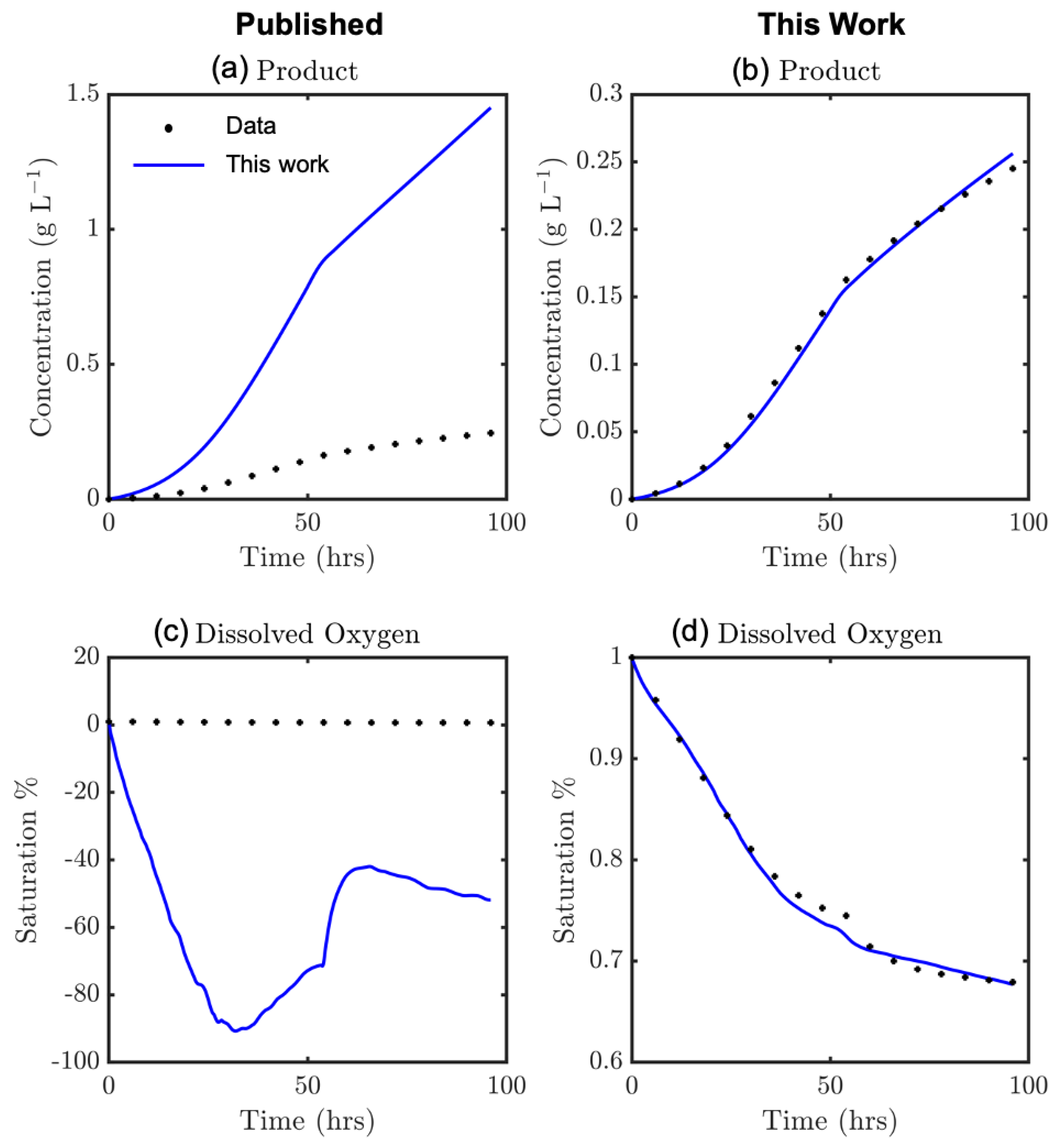
Niu and colleagues (2013, 2016) performed a range of experimental campaigns, gathering state data to facilitate parameter estimation of values which may not be directly measured [39,40]. It was found that there was significant mismatch between certain presented state trajectories (namely product, P and dissolved oxygen content, CO) and those resulting from simulating the model using the entire published parameter set (29 parameters). As a result, a selective parameter re-estimation has been performed for five parameters, which pertain to uptake ratios for oxygen consumption (m_O and Y_X/O) and product formation (µ_P, K_h, Y_P/O). MATLAB’s OPTI Toolbox and the fmincon function was used to minimize the error between state trajectories and the experimental data (Equation (11)), solving for the parameter vector, θ = [m_O Y_X/O µ_P K_h Y_P/O], giving the best fit.

$$\underset{\theta }{\min }{\displaystyle \sum }_i{\displaystyle \sum }_j{\left(\frac{\mathrm{data} - \mathrm{model}}{{\overline{\mathrm{data}}}_i}\right)}^2$$

(11)

The model fit to P and CO profiles vs. experimental data is greatly improved following parameter regression of θ, as shown in Figure 4. The model kinetic parameter values (both fitted and taken from the literature) are listed in

Table 3. Kinetic (published and regressed in this study) and fermentor design parameters.

Kinetic Parameters
Parameter Description	Symbol	Value	Units	Source
Growth pre-exponent	Ag	0.1224	h−1	[40]
Growth energy barrier	Eg	60	kJ mol−1	[40]
Death pre-exponent	Ad	1.9 × 10−3	h−1	[40]
Death energy barrier	Ed	340	kJ mol−1	[40]
Equation (2) constant	K1	1 × 10−10	(–)	[40]
Equation (2) constant	K2	1.3 × 10−4	(–)	[40]
Substrate Contois constant	KS	0.1828	g L−1	[40]
Oxygen Contois constant	KO	0.0352	g L−1	[40]
Maximum substrate concentration	XMAX	0.87	g L−1	[40]
Monod constant	Kd	0.0368	(–)	[40]
Hydrolysis constant	Kh	4.0 × 10−4	h−1	This study a
Substrate maintenance coefficient	mS	0.0624	g g−1 h−1	[40]
Biomass/substrate yield constant	YX/S	0.25	g g−1	[40]
Product/substrate yield constant	YP/S	0.68	g g−1	[40]
Specific production rate	μP	0.05	g g−1 h−1	This study a
Production inhibition constant	KI	0.1	g L−1	[39]
Production inhibition constant	KP	2 × 10−4	g L−1	[39]
Oxygen maintenance coefficient	mO	4.0 × 10−3	g g−1 h−1	This study a
Biomass/oxygen yield constant	YX/O	43.5	g g−1	This study a
Product/oxygen yield constant	YP/O	253.3	g g−1	This study a
Design Parameters
Parameter Description	Symbol	Value	Units	Source
Fermentor volume	VF	100	L	[39,40]
Ventilation rate	Q	3.0	m3 h−1	[39,40]
Agitation speed	n	400	rpm	[39,40]
Stirring power	P	1500	W	[39,40]
Agitator diameter	d	0.01	m	[39,40]
Vessel diameter	D	0.5	m	[39,40]
a Quality of Parameter Fit: Niu et al. (2013, 2016) [39,40] vs. this study
Variable	MSE		SSE
	Niu et al. (2013, 2016) [39,40]	This study	Niu et al. (2013, 2016) [39,40]	This study
Product, P	4.940 × 10–1	6.815 × 10–5	8.398	1.158 × 10−3
Dissolved Oxygen, CO	3.700 × 103	4.280 × 10−5	6.290 × 104	0.728 × 10−3

. Design parameters of the bioreactor are taken as those considered in the literature and are also summarized in Table 3. The improved model fit in product and dissolved oxygen concentrations are also quantified by their corresponding mean squared error (MSE) and sum of squared error (SSE) values for P and CO profiles.

Various model parameters are taken from studies by Niu and colleagues (2013, 2016) on the same experimental apparatus, where errors of their parameter fits on different species concentrations are also reported [39,40]. Our parameter regression showed reduced discrepancy between the experimental and model results. It is important to validate all results presented in this work (both model parameter estimates and dynamic optimization runs) vs. further experimental runs on the apparatus used by Niu and colleagues (2013, 2016) [39,40].

2.2. Dynamic Simulation

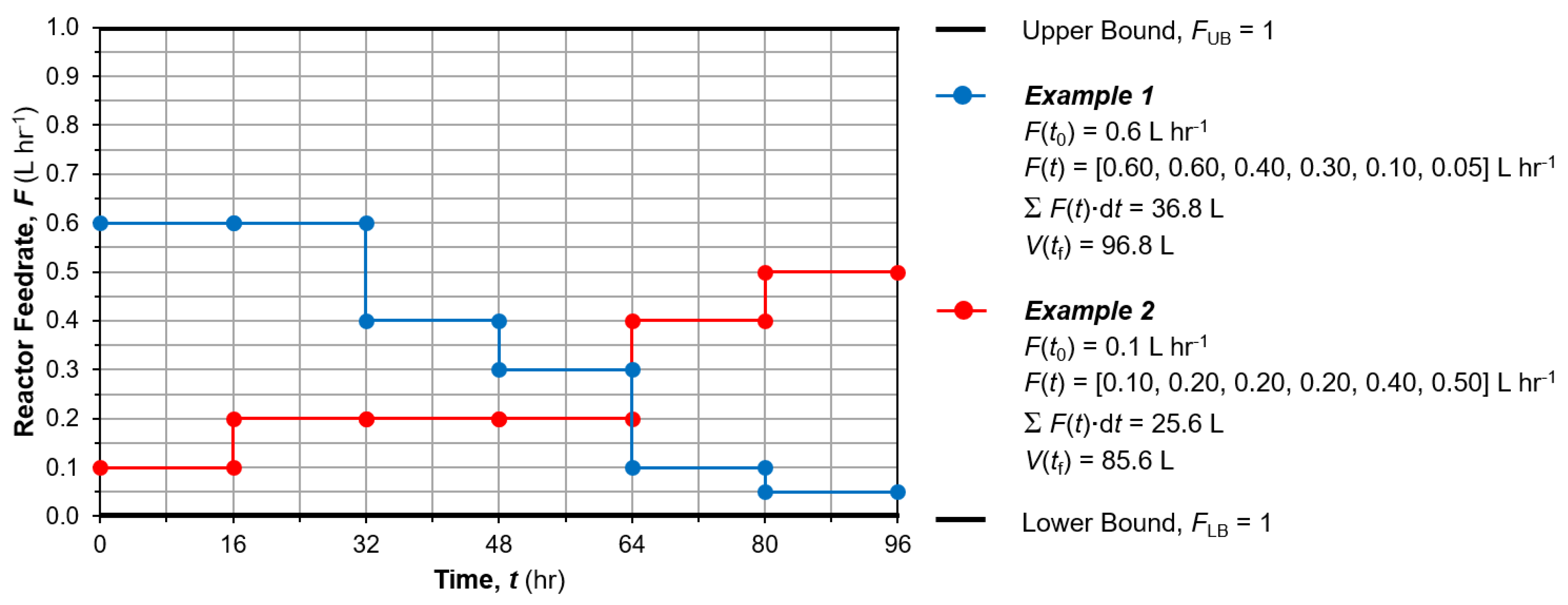
Exploring the entire dynamic operating design space with respect to attainable productivity and reactor performance is useful in order to understand in depth the biochemical system behavior prior to undertaking dynamic optimization [41]. We implement exhaustive dynamic simulation subject to rules and constraints on the possible control (reactor feedrate) profiles over the batch duration to limit the number of simulations and total computational effort [41]. A total possible batch duration of t_f = 96 h is considered (as per the experimental demonstrations [39,40]). The control profiles are considered piecewise constant (PWC) with six temporal elements (N = 6) considered, i.e., a time step of Δt = 16 h. The reactor feed can have initial values considered, F(t = 0) = 0.1:0.1:0.9 L h⁻¹, i.e., nine (9) possible starting values. After each Δt, the change in reactor feed, ΔF = {0, ±0.1, ±0.2, ±0.3, ±0.4} L h⁻¹. Profiles which result in F(t) < 0 or F(t) > 1 (= feedrate bounds), as well as cases where V(t) > 100 (= fermentation vessel volume) are not considered to respect the bounds imposed as per the experimental demonstration [39,40]. Figure 5 shows an example of two possible reactor feedrate profiles considered within the dynamic simulation, with all of the abovementioned restrictions met. The resulting number of feed profiles considered for dynamic simulation = 625,331. The effects of different feed profiles on state variables and different trade-offs therein are then considered. Thereafter, mathematical dynamic optimization is performed in order to elucidate the optimal reactor feedrate policy to maximize nosiheptide production.

2.3. Dynamic Optimization

2.3.1. Problem Statement

Determining how any industrial production process shall be operated efficiently typically involves mathematical optimization of some form [42]. Often this will include an optimal control problem, where a system of state variables [x] are influenced by an externally-manipulated control variable, u, so the optimal control vector u(t) is sought to minimize an objective, φ. Considering a generic problem where no running payoff is considered (the objective, Equation (12), evaluated at terminal time only), the dynamic optimization problem can be defined as follows [43,44].

$$\underset{u\left(t\right), t_{\mathrm{f}}}{\min }\phi (x\left(t_{\mathrm{f}}\right), t_{\mathrm{f}})$$

(12)

$$\frac{\mathrm{d}x}{\mathrm{d}t}=f \left(x\left(t\right), u\left(t\right)\right)$$

(13)

x(t₀) = x₀

(14)

h (x(t), u(t)) = 0, g (x(t), u(t)) ≤ 0

(15)

h_f (x(t_f)) = 0

(16)

g_f (x(t_f)) ≤ 0

(17)

u_L ≤ u(t) ≤ u_U

(18)

x_L ≤ x(t) ≤ x_U

(19)

The ordinary differential equations (ODEs) which dictate the state trajectories (Equation (13)) are influenced at any time by the current control (u) value, with initial state conditions given by Equation (14). Equation (15) represents equality and inequality constraints across the entire time horizon, t ∈ [t₀, t_f], with terminal constraints given by Equations (16) and (17). Lastly, the state and control boundaries are constrained within permissible bounds by Equations (18) and (19).

2.3.2. Solution Method

A wide range of methodologies exist for solving an optimal control trajectory problem, including variation methods and finite approximation methods [41,45]. In the former, exploiting Pontryagin’s maximum principle allows the resulting two-point boundary value problem to be solved, while the latter uses predefined functional forms to represent the control profile [46]. Finite formulations may be tackled with simultaneous, sequential, or multi shooting strategies which are extensively reviewed in the literature [43]. The sequential strategy involves discretization of the control profile with the ODE system (process model), requiring regular re-integration during the algorithm to compute corresponding state trajectories, an approach effective for problems with few decision variables and constraints [47], which has been widely applied to engineering problems [48,49,50]. In contrast, simultaneous strategies require the ODE system to also be discretized on the time horizon to produce a large-scale nonlinear programming (NLP) problem requiring no further integration of the differential algebraic equation (DAE) system, generally using orthogonal collocation techniques. The latter offers numerous benefits, being faster to solve and able to handle problems with a greater number of decision variables and constraints [51,52].

A direct method for dynamic optimization (simultaneous strategy) is performed. Orthogonal polynomials on finite elements are used to approximate the control and state trajectories, allowing the continuous problem to be converted to NLP form. The DAE system is converted to a system of algebraic equations (AEs), where decision variables of the derived NLP problem are the coefficients of the linear combinations of these AEs. Precision varies with collocation point locations and step sizes used [53,54].

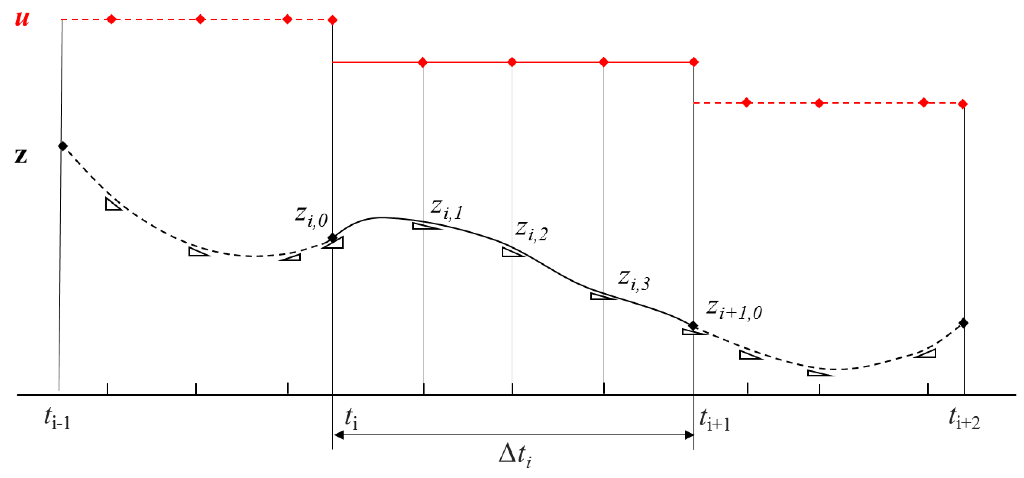
Consider the general problem with N elements (i = 1, …, N), each of which has K collocation points (j = 1, …, K). The differential profiles (Equation (13)) can be approximated by Equation (20), where Δt_i is the length of element i and dx/dt_i,j is the derivative of the state variable in element i at the j^th collocation point. Ω_j is a j^th order polynomial satisfying Equation (21). Continuity of the state trajectories is ensured by Equation (22). The control profile is approximated by Equation (23), where ψ_j is a Lagrange polynomial of degree K that satisfies ψ_j (ρ_j) = δ_j for j = 1, …, K. It is shown in Figure 6 how control variables may have discontinuities at element boundaries, while continuity in states at these same boundaries is produced. In doing so, the continuous general problem has been reduced to a discreet DAE system, which can be solved by a suitable NLP subroutine.

$$x_i{=x}_{i-1}+\Delta t_i{\displaystyle \sum }_{j=1}^K{\Omega }_j\left(\frac{{t - t}_{i-1}}{ \Delta t_i}\right)\frac{\mathrm{d}x}{{\mathrm{d}t}_{i,j}}$$

(20)

$${\Omega }_j\left(0\right)=0,{\Omega }_j^{\prime }\left({\rho }_j\right)={\delta }_j \mathrm{for}j=1,\dots ,K$$

(21)

$$x\left(t\right){=x}_{i-1}+\Delta t_i{\displaystyle \sum }_{j=1}^K{\Omega }_j\left(1\right)\frac{\mathrm{d}x}{{\mathrm{d}t}_{i,j}}$$

(22)

$$u\left(t\right)={\displaystyle \sum }_{j=1}^K{\psi }_j\left(\frac{{t - t}_{i-1}}{ \Delta t_i}\right)u_{i,j}$$

(23)

2.3.3. Optimization Objectives and Strategy

There are two obvious objectives for optimal fermentation: reduced batch duration and maximum productivity (even if this requires later dilution, it is desirable to enhance yield). A bi-objective problem is considered, defined by Equations (24)–(26). Multiple optimization objectives can also be formulated as a single objective function by considering a sum of weighted individual objectives as in other studies by our group [21,41]; however, such methods can be used in studies considering full-scale industrial operation with ample experimental and dynamic production data acquisition, whereas for comparison of modeling and optimization results vs. a relatively small experimental dataset (as is the case here), a bi-objective problem defined as a product of individual objectives is more appropriate. Constraints impose bounds on the control profiles (Equations (27)–(29) as well as the broth volume being limited by the reactor size (Equation (30)).

$$\underset{T\left(t\right), \mathit{pH}\left(t\right), F\left(t\right)}{\min } f_1 f_2$$

(24)

f₁ = t_f

(25)

f₂ = −V(t_f) P(t_f)

(26)

299 ≤ T(t) ≤ 305  for t ∈ [t₀, t_f]

(27)

6 ≤ pH(t) ≤ 8  for t ∈ [t₀, t_f]

(28)

0 ≤F(t) ≤ 1  for t ∈ [t₀, t_f]

(29)

V(t) ≤ 100  for t ∈ [t₀, t_f]

(30)

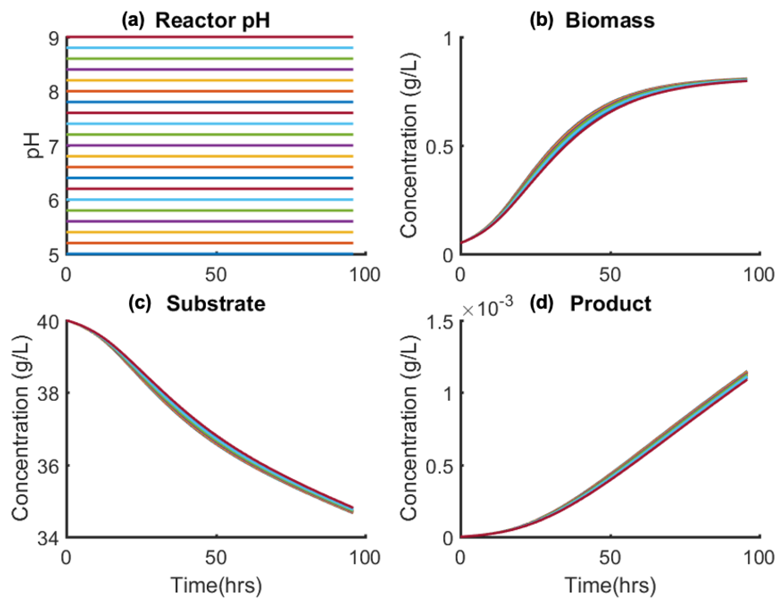
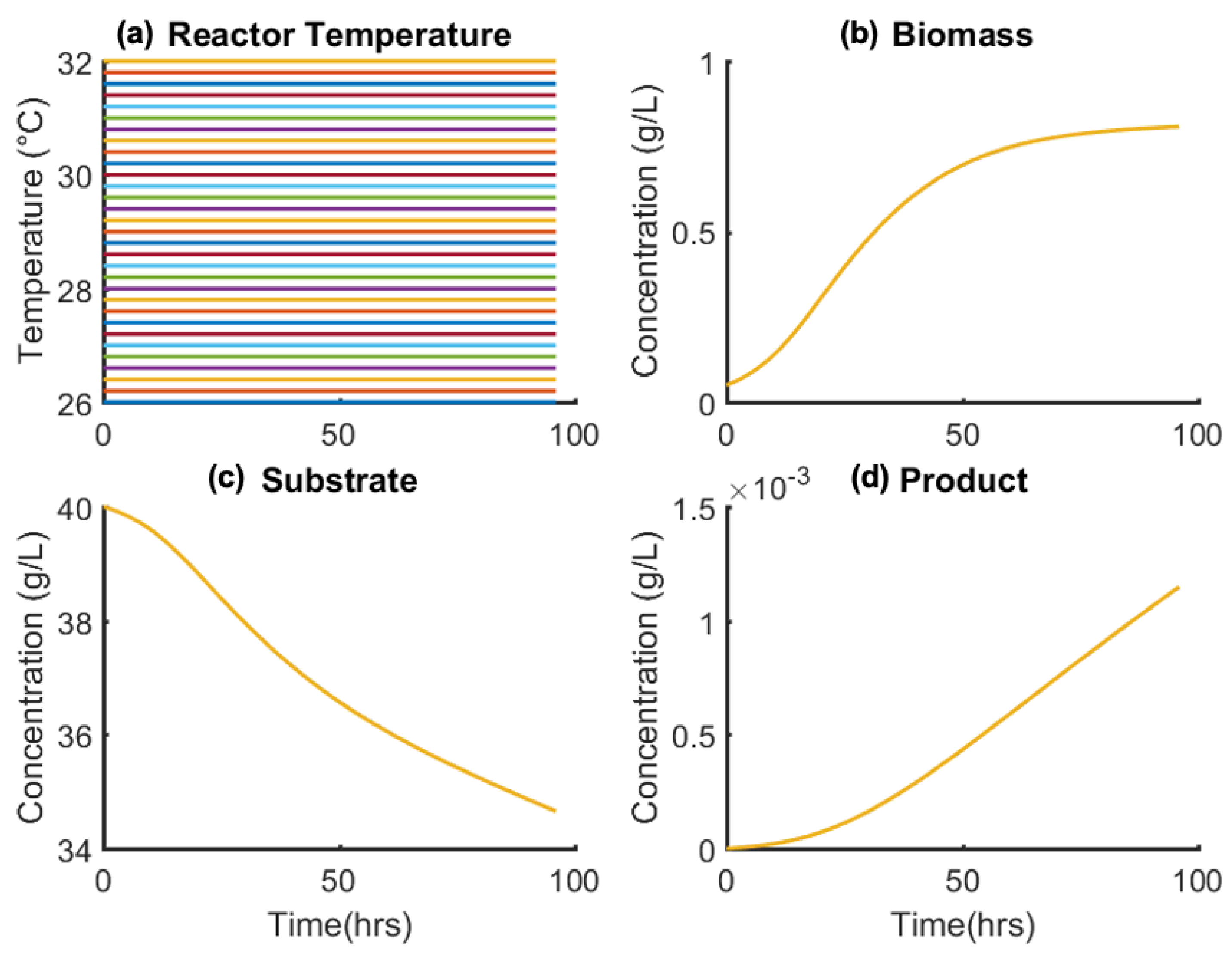
To elucidate the sensitivity of the model states on manipulated controls (F, T, pH), a sensitivity analysis was performed. Figure 7 shows the effect of varying constant reactor pH on state profiles, showing negligible variation over the applicable pH(t) = 6–8 (Equation (28)); this is due to the pH-dependent model term (Equation (2)) varying weakly vs. pH for the given model parameters (K₁ and K₂). Similarly, the sensitivity of states vs. isothermal reactor temperature (T(t) = 26–32 °C) is compared in Figure 8. The variation in states vs. temperature is also negligible due to biomass cell growth and death (numerators of first terms in Equations (2) and (3), respectively,) varying weakly vs. temperature within the applicable range. The model dependence of both temperature and pH is as presented in the literature [39,40].

We illustrate effects to justify selection of only reactor feeding as manipulation variable for dynamic optimization. It is possible that the growth peak occurs at a higher temperature than the range of values considered here (bounds chosen to ensure model parameters are commensurate with experiments), which should be confirmed via experiments in the same apparatus as that described by Niu and colleagues (2013, 2016) [39,40].

The results of the sensitivity analysis imply that it is logical to remove temperature and pH profiles from the optimization problem to reduce the problem size compared to optimizing all three controls simultaneously. Reactor temperature and pH are fixed as per the literature (see

Table 4. Fixed operating and initial state conditions as per the original experimental study [39,40].

Operating Variable
Variable	Symbol	Initial Value	Units
Temperature	T(t0) = T(t)	30	°C
pH	pH(t0) = pH(t)	7	(–)
State Initial Condition
Variable	Symbol	Initial Value	Units
Biomass loading	X (t0)	0.05	g L−1
Substrate concentration	S (t0)	40	g L−1
Product concentration	P (t0)	0	g L−1
Culture volume	V (t0)	60	L
Dissolved oxygen content	CO (t0)	0.037	g L−1

) to ensure healthy biomass and allowing the feed profile to be optimized in isolation. Initial conditions for state variables are assumed to be as in the literature and are also summarized in Table 4.

Any multi-objective problem, such as that defined by Equation (24), will not have a single solution, but rather an entire optimal front upon which no single objective can be improved without sacrificing another, i.e., a Pareto front. Numerous approaches can be used to modify a multi-objective problem for compatibility with single objective methods such as that proposed in Section 2. Commonly, a weighted sum objective is used to combine the competing objectives into a single term with weights defining the relative importance of each. However, weights assigned to the multiple process targets to produce a single objective function may be considered arbitrary, with decision-makers not necessarily able to quantify a priori the relative importance of the competing objectives. Rather, we elect to consider an ε-constraint approach. One of the objectives can be considered as a constraint in the problem formulation, solving the other to optimality. This is repeated by incrementally increasing the ε-constraint value across the entire span of permissible values for that objective. Here, the batch time is treated as the secondary objective and converted to a constraint (Equations (31) and (32)).

$$\underset{F\left(t\right)}{\min }-V(t_{\mathrm{f}}) P(t_{\mathrm{f}})$$

(31)

t_f = ε

(32)

Solving this modified problem across a range of values for ε produces a Pareto front of optimal solutions, allowing the trade-off to be visualized and used for process design and operation decisions. Generally, Equation (32) would be an inequality constraint in the ε-constrained multi-objective method; however, so as to visualize the performance drop observed in excessively long batches an equality term is used. Doing so enforces the specific batch time in each case, in place of converging to the optimal batch length with little indication of the responsible mechanism. We consider ε = {120, 200, 205, 275, 390} h and N = 20.

3. Results and Discussion

3.1. Dynamic Simulation and Design Space Visualization

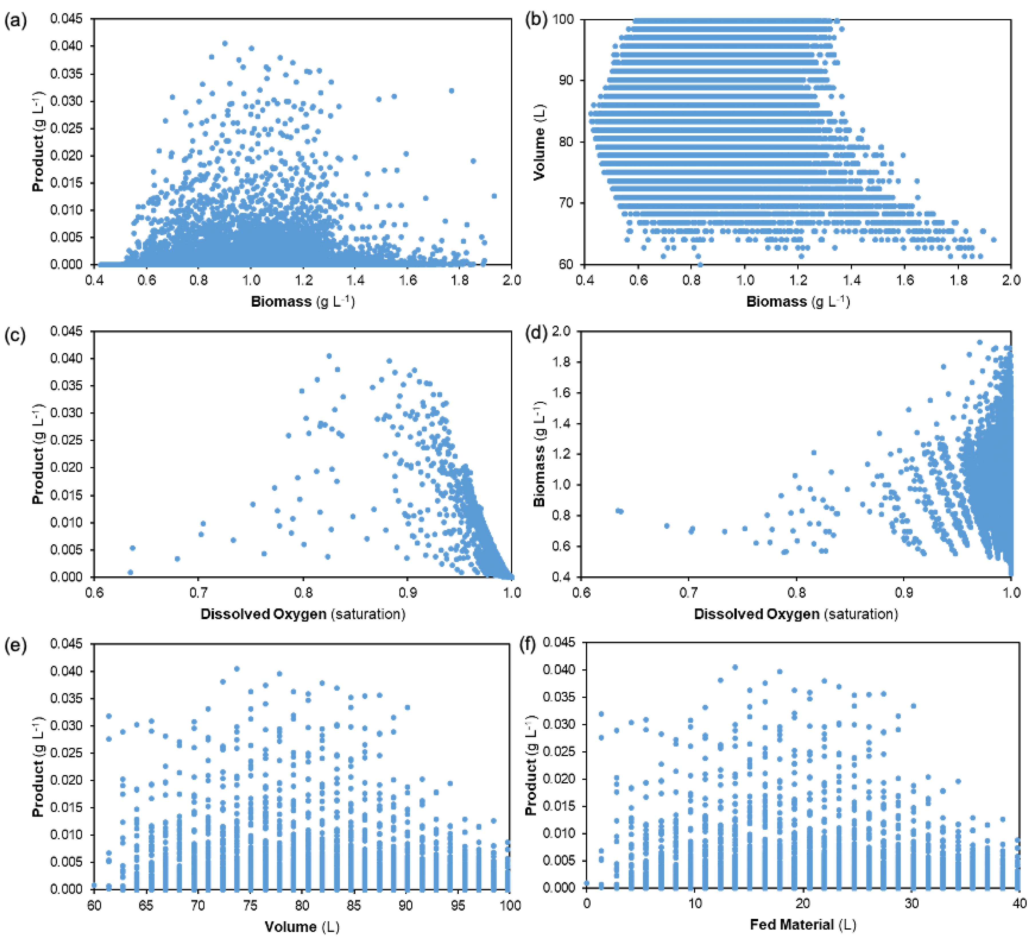
Figure 9 presents trade-offs between different state variables from the range of reactor feedrate profiles for dynamic simulation purposes. The following comparisons are made: product vs. remaining biomass, volume vs. biomass, product and biomass vs. dissolved oxygen, and product vs. fermentation broth volume and total amount of fed material during fed-batch production (= Σ F(t)Δt). Various trade-offs and trends between states are observed.

Observing the attained product concentrations vs. biomass at the end of the batch duration shows that the highest productivities are attained from intermediate biomass values, not necessarily from the highest. It is also observed that many of the considered feedrate profiles achieve comparably low productivities for their given biomass present, highlighting the need for process optimization. Resulting broth volumes are also highest at the low to intermediate range of biomass concentrations; it should be noted that the model assumes that biomass growth does not affect broth volume, i.e., that the system is relatively dilute. For adaptation to systems with higher biomass loading, Equation (7) should contain a term that describes volumetric changes due to biomass growth.

Biomass concentrations are highest when the system is near oxygen saturation due to cells requiring oxygen for growth. Most of the considered reactor feedrate profiles approach oxygen saturation; however, the maximum productivities are obtained for profiles with lower dissolved oxygen content. The highest product concentrations are observed for intermediate values of reactor feedrates/final broth volumes. Banding is observed in the product vs. volume/fed material plots due to the discrete initialized values and step changes employed for dynamic simulation (see Section 2.2).

Figure 9 shows that the highest nosiheptide product concentrations are attained with very particular reactor feedrate profiles, i.e., the system performance is very sensitive to the considered reactor feedrate profiles. This design space investigation and visualization via dynamic simulation provides an incentive for dynamic optimization to systematically establish the optimum feed profile. Dynamic simulation results show performances attained for t_f = 96 h (the batch duration as per experimental studies [39,40]); the effect of varying batch time is another dynamic optimization goal.

3.2. Optimal Reactor Reactor Feedrate Policy

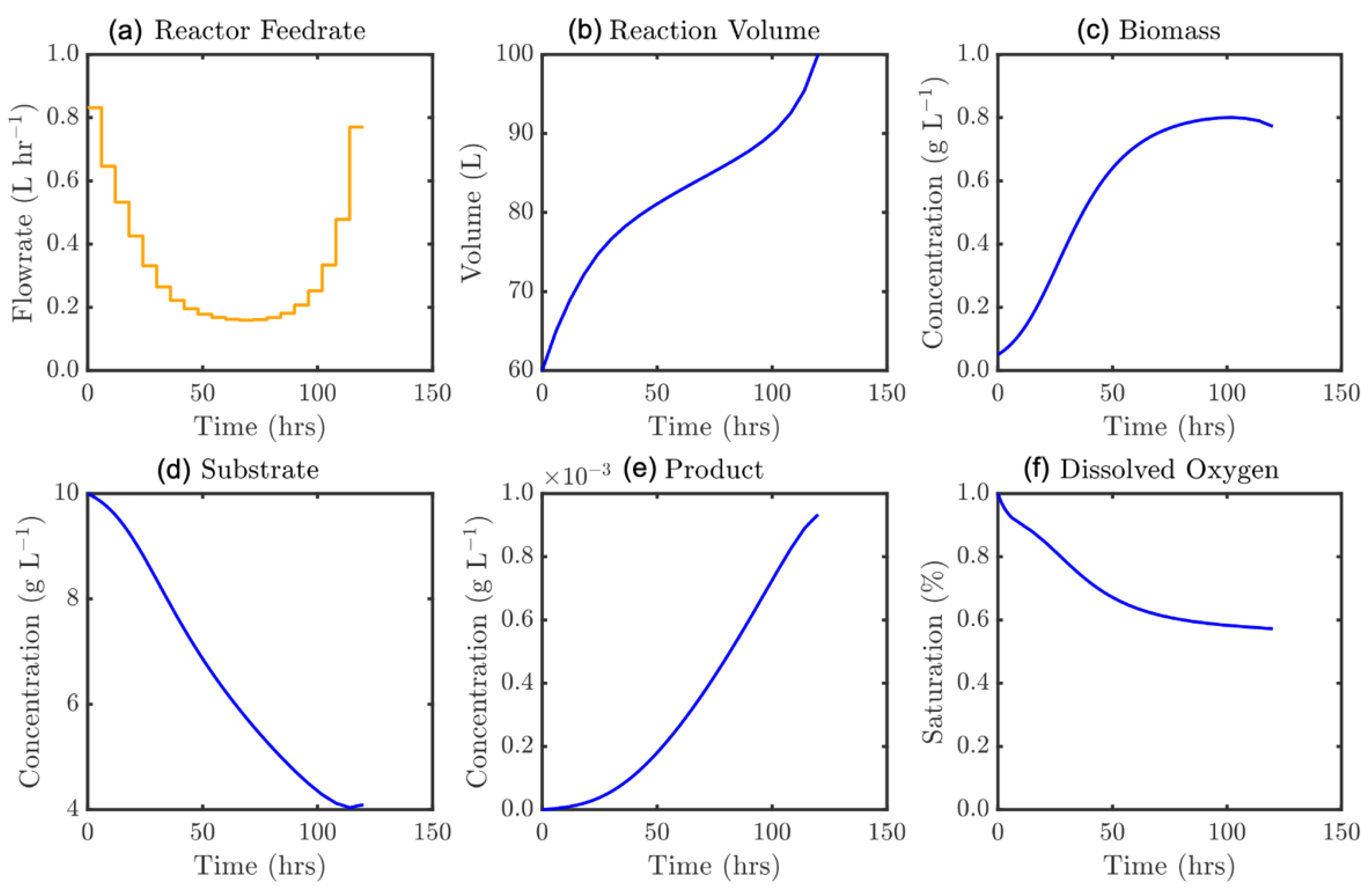
The resultant large-scale NLP problem from DynOpt is solved for each instance using IPOPT (Interior Point OPTimizer) [51,52] and global optimality is ensured with a multi-start search via Latin hypercube sampling of the input space for initialization. Analytical state and control Jacobians, in addition to the objective gradients, are explicitly defined and provided to the solver which drastically improves runtime due to far fewer function evaluations being required. The problem defined by Equations (31) and (32) has been solved for a range of instances, considering an array of initialization strategies (initial control profile ‘guesses’) as well as for increasing time domain discretization, defined by the number of control segments, N. Solution attainment is robust with little sensitivity to the initialization strategy employed, as has been in the case in other dynamic simulation and optimization studies on biochemical systems implemented by our group [55]. The performance of the IPOPT NLP solver was compared to the default solver within MATLAB’s OPTI Toolbox (fmincon), with IPOPT equaling or outperforming in all instances. The single objective solution is shown in Figure 10 where N = 12 and batch time t_f = 120 h.

It is demonstrated that optimal feed trajectory computed is a novel parabolic form. This efficient strategy initially feeds substrate at a high rate, assisting with the biomass development towards its maximum value. Lowering this over the first portion of the process prevents restrictive dilution of both the biomass and the early product formation. After sustaining a feedrate near 0.2 g L⁻¹ until the maximum biomass concentration is approached, the feedrate is increased exponentially towards the end of the process, capitalizing on the reduced inhibition given that less substrate is now present in the broth. It is noteworthy that the solution suggests the reactor should only be entirely full (V = 100 L) at the very end of the process. The multi-objective Pareto front of optimal solutions is presented in Figure 11 where batch time as a secondary objective was constrained by increments of 5 h between 100 and 400 h according to Equation (32).

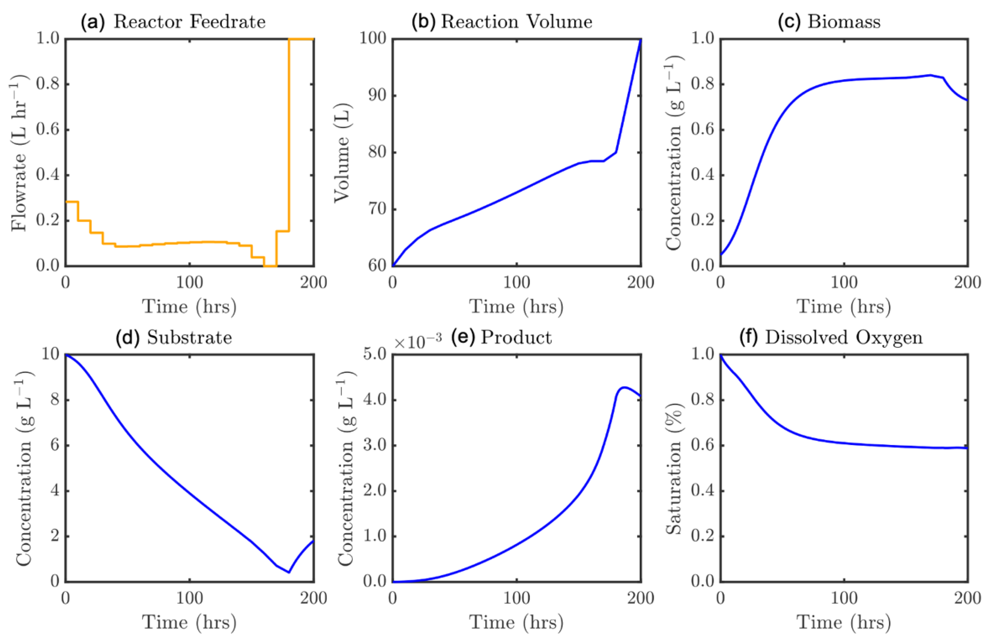
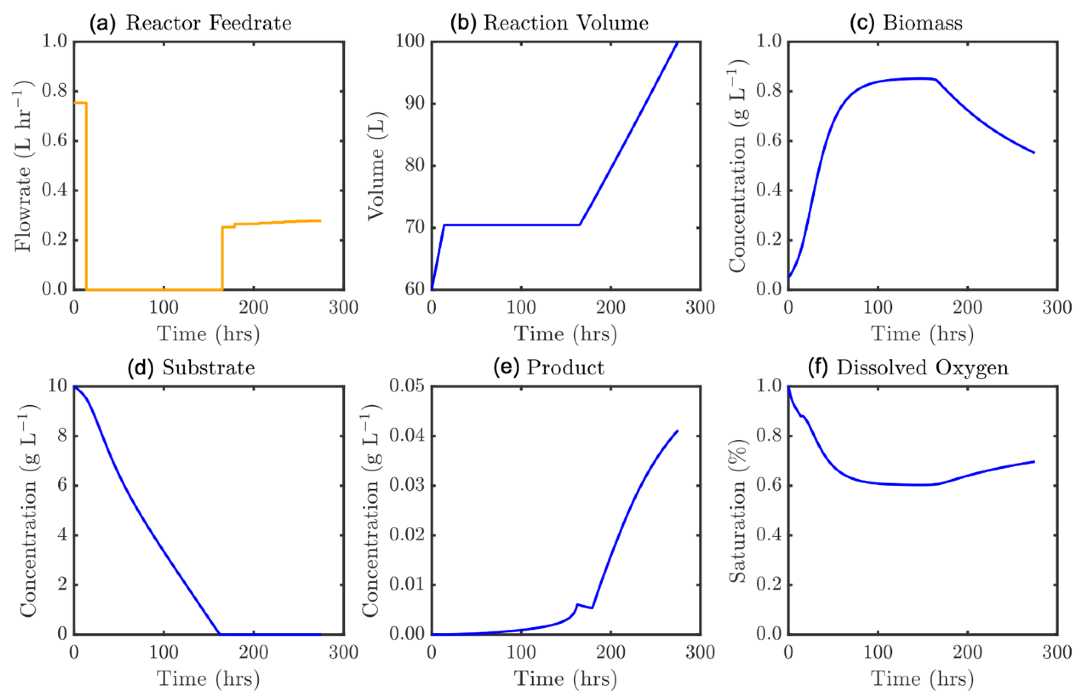
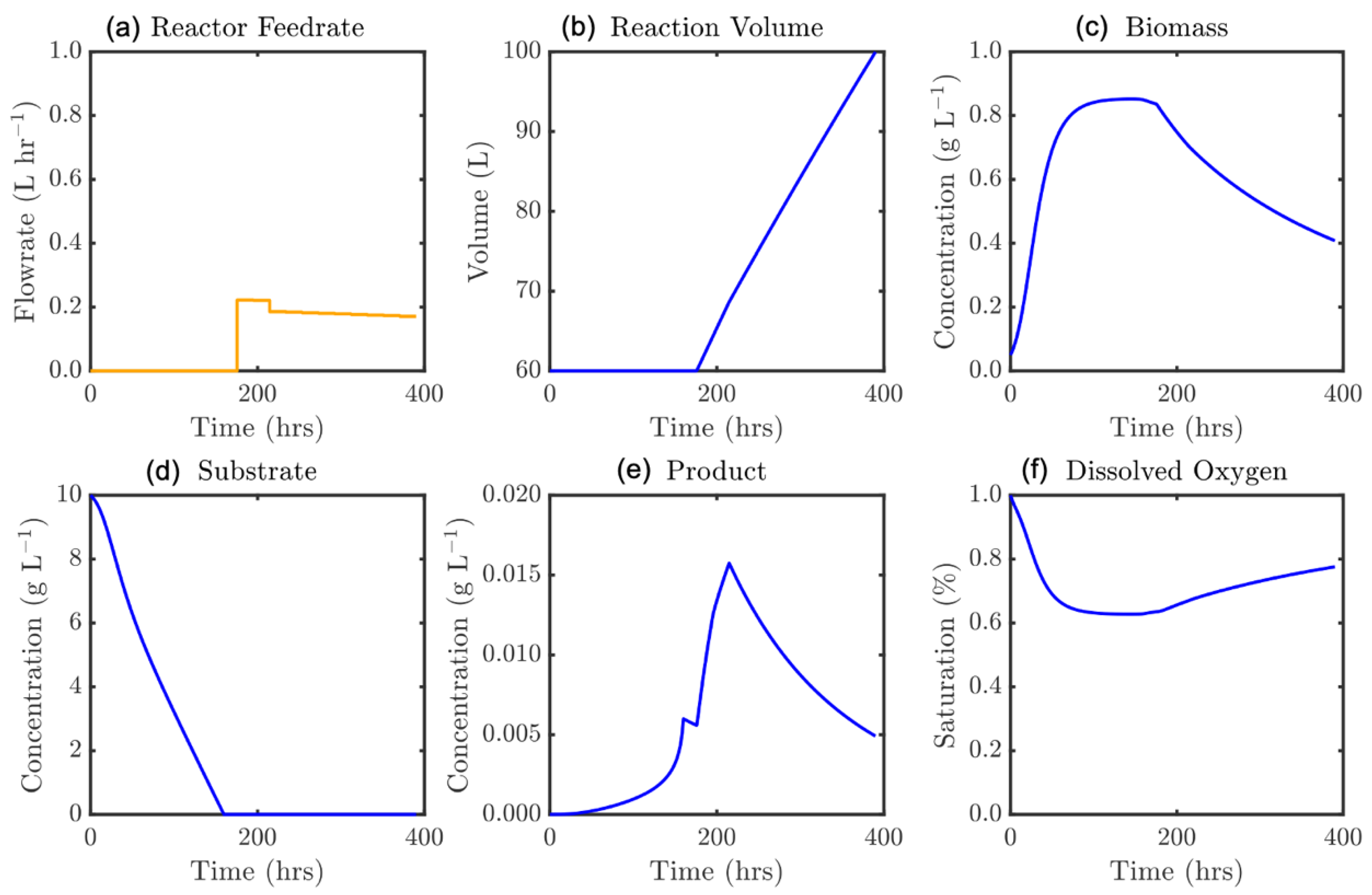
Three distinct regions on the Pareto plot (Figure 11) can be identified. In the left-most region (100–200 h) a near linear relationship exists between attainable product mass and permitted batch time. At batch time, t_f > 200 h, a dramatic shift is observed, whereby a much larger product mass is produced. This continually increases at a less than linear rate until a maximum production is observed when t_f ≈ 330 h. After this a dramatic drop in production is shown when batch time is excessively long. To better understand these observed trends, solution profiles of the model states corresponding to the solutions on the Pareto plot can be inspected. Figure 12 represents the solution for the scenario t_f = 200 h, with the same for t_f = 205 h shown in Figure 13.

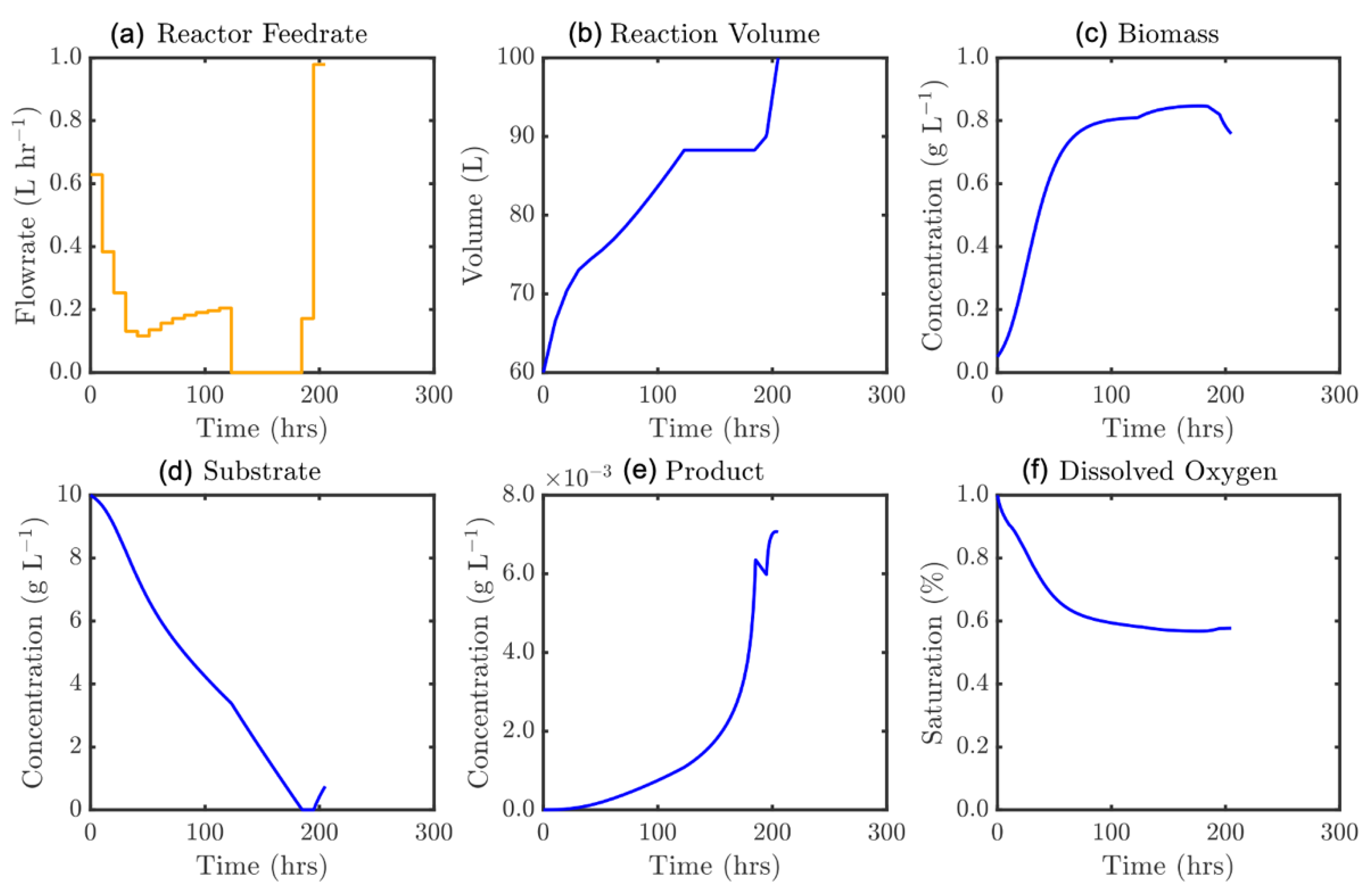
Figure 12 shows similar behavior to Figure 10: initially promoting biomass growth before lowering the feedrate for the intermediate batch portion, prior to increasing substrate feed to capitalize on the favorable reactor state. The large transition in Figure 10 may be understood from the t_f = 205 h solution (Figure 13). This represents the first time at which the initial reactor substrate content is completely consumed. This allows the substrate to deplete (feeding biomass growth and maintenance), and the moment that the substrate concentration approaches zero the feedrate is drastically increased. In doing so there is essentially no inhibitory mechanism and extremely efficient fermentation may be performed for the remainder of the batch, generating an elevated mass of product. This is similarly observed in Figure 14 for ε = 275 h, with a sustained feed period at the end of the process at a precise level to prevent accumulation while still feeding rapid product growth.

Figure 15 highlights the mechanism for the performance drop once the batch time becomes excessively long. Here the batch time is too long for the finite reactor volume and substrate mass that may be fed. Now the product hydrolysis becomes prohibitive with the nosiheptide produced earlier being later consumed, where overfilling the reactor would be necessary to maintain a production rate greater than the hydrolysis rate in the late stages of the process. As such, a critical batch time is identified, after which yield is reduced. This also highlights that the product state must be rapidly changed once the maximum production is observed, to prevent undesirable product losses.

Care must be taken when interpreting these results. The optimal scenario appears to be to promote biomass growth prior to depleting the substrate concentration entirely, after which further substrate additions may be instantly converted to nosiheptide in the absence of an accumulated inhibitory substrate content in the reactor. While the model authors do not suggest the model is not valid under these conditions, the portion of their data used in the parameterization, which is presented in the corresponding publications, do not show such behavior. The model validity under these conditions (no substrate accumulated) must first be ensured. The considered dynamic fed-batch fermentation model for nosiheptide production was developed by Niu and colleagues (2013, 2016) and based on their experimental setup [39,40]. While experimental runs are out of the scope of this study, it is important to validate regressed model parameters and corroborate dynamic optimization results presented here with experimental campaigns of the pilot fermentation process.

4. Conclusions

The fed-batch production of nosiheptide is considered to circumvent mass transfer inhibition at excessive substrate concentrations in the fermentation broth, where the reactor is only partially filled initially and substrate supplemented over time. Design space investigation and visualization via dynamic simulation of a large set of possible reactor feedrate profiles illustrated trade-offs and the need for systematic dynamic optimization due to the high process sensitivity to the chosen reactor feedrate policy. Dynamic optimization has been performed for minimization of batch time and inverse yield (for maximization). An ε-constraint approach has been implemented, treating batch time as a secondary objective which is converted to an inequality constraint that is gradually relaxed as the problem is re-solved to maximize nosiheptide production. Orthogonal polynomials on finite elements are used to approximate the control and state trajectories allowing the continuous problem to be converted to NLP form. Optimal operation requires the feedrate to be manipulated in such a way that the inhibitory mechanism of the substrate can be avoided; however, the model validity under these conditions (no substrate accumulated) must first be ensured to realize these results.

References

- Zaffiri, L.; Gardner, J.; Toledo-Pereyra, L.H. History of antibiotics. from salvarsan to cephalosporins. J. Investig. Surg. 2012, 25, 67–77. [Google Scholar] [CrossRef]
- Russell, M.G.; Jamison, T.F. Seven-step continuous flow synthesis of linezolid without intermediate purification. Angew. Chem. Int. Ed. 2019, 58, 7678–7681. [Google Scholar] [CrossRef] [PubMed]
- Lin, H.; Dai, C.; Jamison, T.F.; Jensen, K.F. A rapid total synthesis of ciprofloxacin hydrochloride in continuous flow. Angew. Chem. Int. Ed. 2017, 56, 8870–8873. [Google Scholar] [CrossRef] [PubMed]
- Volpato, G.; Rodrigues, R.C.; Fernandez-Lafuente, R. Use of enzymes in the production of semi-synthetic penicillins and cephalosporins: Drawbacks and perspectives. Curr. Med. Chem. 2010, 17, 3855–3873. [Google Scholar] [CrossRef] [PubMed]
- Benazet, F.; Cartier, M.; Florent, J.; Godard, C.; Jung, G.; Lunel, J.; Mancy, D.; Pascal, C.; Renaut, J.; Tarridec, P.; et al. Nosiheptide, a sulfur-containing peptide antibiotic isolated from Streptomyces actuosus 40037. Experientia 1980, 36, 414–416. [Google Scholar] [CrossRef]
- Wojtas, K.P.; Riedrich, M.; Lu, J.Y.; Winter, P.; Winkler, T.; Walter, S.; Arndt, H.D. Total synthesis of nosiheptide. Angew. Chem. Int. Ed. 2016, 55, 9772–9776. [Google Scholar] [CrossRef]
- Jolliffe, H.G.; Gerogiorgis, D.I. Technoeconomic optimization of a conceptual flowsheet for continuous separation of an analgaesic active pharmaceutical ingredient (API). Ind. Eng. Chem. Res. 2017, 56, 4357–4376. [Google Scholar] [CrossRef] [Green Version]
- Gerogiorgis, D.I.; Jolliffe, H.G. Continuous pharmaceutical process engineering and economics. Investigating technical efficiency, environmental impact + economic viability. Chem. Today 2015, 33, 29–32. [Google Scholar]
- Yu, Y.; Duan, L.; Zhang, Q.; Liao, R.; Ding, Y.; Pan, H.; Wendt-Pienkowski, E.; Tang, G.; Shen, B.; Liu, W. Nosiheptide biosynthesis featuring a unique indole side ring formation on the characteristic thiopeptide framework. ACS Chem. Biol. 2009, 4, 855–864. [Google Scholar] [CrossRef] [Green Version]
- Shirahata, H.; Diab, S.; Sugiyama, H.; Gerogiorgis, D.I. Dynamic modelling, simulation and economic evaluation of two CHO cell-based production modes towards developing biopharmaceutical manufacturing processes. Chem. Eng. Res. Des. 2019, 150, 218–233. [Google Scholar] [CrossRef]
- Veterinary Antimicrobial Resistance and Sales Surveillance 2018. Available online: https://www.gov.uk/government/publications/veterinary-antimicrobial-resistance-and-sales-surveillance-2018 (accessed on 6 March 2020).
- Gonçalves, L.R.B.; Sousa, R.; Fernandez-Lafuente, R.; Guisan, J.M.; Giordano, R.L.C.; Giordano, R.C. Enzymatic synthesis of amoxicillin: Avoiding limitations of the mechanistic approach for reaction kinetics. Biotechnol. Bioeng. 2002, 80, 622–631. [Google Scholar] [CrossRef] [PubMed]
- Gonçalves, L.R.B.; Giordano, R.L.C.; Giordano, R.C. Mathematical modeling of batch and semibatch reactors for the enzymic synthesis of amoxicillin. Process. Biochem. 2005, 40, 247–256. [Google Scholar] [CrossRef]
- Chow, Y.; Li, R.; Wu, J.; Puah, S.M.; New, S.W.; Chia, W.Q.; Lie, F.; Rahman, T.M.R.; Choi, W.J. Modeling and optimization of methanol as a cosolvent in amoxicillin synthesis and its advantage over ethylene glycol. Biotechnol. Bioprocess. Eng. 2007, 12, 390–398. [Google Scholar] [CrossRef]
- Silva, J.A.; Costa Neto, E.H.; Adriano, W.S.; Ferreira, A.L.O.; Gonçalves, L.R.B. Use of neural networks in the mathematical modelling of the enzymic synthesis of amoxicillin catalysed by penicillin G acylase immobilized in chitosan. World J. Microbiol. Biotechnol. 2008, 24, 1761–1767. [Google Scholar] [CrossRef]
- McDonald, M.A.; Bommarius, A.S.; Rousseau, R.W.; Grover, M.A. Continuous reactive crystallization of β-lactam antibiotics catalyzed by penicillin G acylase. Part I: Model development. Comput. Chem. Eng. 2019, 123, 331–343. [Google Scholar] [CrossRef]
- McDonald, M.A.; Bommarius, A.S.; Grover, M.A.; Rousseau, R.W. Continuous reactive crystallization of β-lactam antibiotics catalyzed by penicillin G acylase. Part II: Case study on ampicillin and product purity. Comput. Chem. Eng. 2019, 126, 332–341. [Google Scholar] [CrossRef]
- Cuthbertson, A.B.; Rodman, A.D.; Diab, S.; Gerogiorgis, D.I. Dynamic modelling and optimisation of the batch enzymatic synthesis of amoxicillin. Processes 2019, 7, 318. [Google Scholar] [CrossRef] [Green Version]
- Encarnación-Gómez, L.G.; Bommarius, A.S.; Rousseau, R.W. Crystallization kinetics of ampicillin using online monitoring tools and robust parameter estimation. Ind. Eng. Chem. Res. 2016, 55, 2153–2162. [Google Scholar] [CrossRef]
- McDonald, M.A.; Bommarius, A.S.; Rousseau, R.W. Enzymatic reactive crystallization for improving ampicillin synthesis. Chem. Eng. Sci. 2017, 165, 81–88. [Google Scholar] [CrossRef]
- Dafnomilis, A.; Diab, S.; Rodman, A.D.; Boudouvis, A.G.; Gerogiorgis, D.I. Multi-objective dynamic optimization of ampicillin batch crystallization: Sensitivity analysis of attainable performance vs. product quality constraints. Ind. Eng. Chem. Res. 2019, 58, 18756–18771. [Google Scholar] [CrossRef]
- Schroën, C.G.P.H.; Nierstrasz, V.A.; Moody, H.M.; Hoogschagen, M.J.; Kroon, P.J.; Bosma, R.; Beeftink, H.H.; Janssen, A.E.M.; Tramper, J. Modeling of the enzymatic kinetic synthesis of cephalexin-influence of substrate concentration and temperature. Biotechnol. Bioeng. 2001, 73, 171–178. [Google Scholar] [CrossRef] [PubMed]
- Schroën, C.G.P.H.; Fretz, C.B.; DeBruin, V.H.; Berendsen, W.; Moody, H.M.; Roos, E.C.; VanRoon, J.L.; Kroon, P.J.; Strubel, M.; Janssen, A.E.M.; et al. Modelling of the enzymatic kinetically controlled synthesis of cephalexin: Influence of diffusion limitation. Biotechnol. Bioeng. 2002, 80, 331–340. [Google Scholar] [CrossRef] [PubMed]
- Travascio, P.; Zito, E.; De Maio, A.; Schroën, C.G.P.H.; Durante, D.; De Luca, P.; Bencivenga, U.; Mita, D.G. Advantages of using non-isothermal bioreactors for the enzymatic synthesis of antibiotics: The penicillin G acylase as enzyme model. Biotechnol. Bioeng. 2002, 79, 334–346. [Google Scholar] [CrossRef] [PubMed]
- McDonald, M.A.; Marshall, G.D.; Bommarius, A.S.; Grover, M.A.; Rousseau, R.W. Crystallization kinetics of cephalexin monohydrate in the presence of cephalexin precursors. Cryst. Growth Des. 2019, 19, 5065–5074. [Google Scholar] [CrossRef]
- Farkya, S.; Bisaria, V.S.; Srivastava, A.K. Biotechnological aspects of the production of the anticancer drug podophyllotoxin. Appl. Microbiol. Biotechnol. 2004, 65, 504–519. [Google Scholar] [CrossRef] [PubMed]
- Laursen, S.Ö.; Webb, D.; Ramirez, W.F. Dynamic hybrid neural network model of an industrial fed-batch fermentation process to produce foreign protein. Comput. Chem. Eng. 2007, 31, 163–170. [Google Scholar] [CrossRef]
- Truppo, M.D.; Pollard, D.J.; Moore, J.C.; Devine, P.N. Production of (S)-γ-fluoroleucine ethyl ester by enzyme mediated dynamic kinetic resolution: Comparison of batch and fed batch stirred tank processes to a packed bed column reactor. Chem. Eng. Sci. 2008, 63, 122–130. [Google Scholar] [CrossRef]
- Xing, Z.; Bishop, N.; Leister, K.; Li, Z.J. Modeling kinetics of a large-scale fed-batch CHO cell culture by Markov chain Monte Carlo method. Biotechnol. Prog. 2010, 26, 208–219. [Google Scholar] [CrossRef]
- Song, H.; Eom, M.H.; Lee, S.; Lee, J.; Cho, J.H.; Seung, D. Modeling of batch experimental kinetics and application to fed-batch fermentation of Clostridium tyrobutyricum for enhanced butyric acid production. Biochem. Eng. J. 2010, 53, 71–76. [Google Scholar] [CrossRef]
- Georgakis, C. Design of dynamic experiments: A data-driven methodology for the optimization of time-varying processes. Ind. Eng. Chem. Res. 2013, 52, 12369–12382. [Google Scholar] [CrossRef]
- Kiparissides, A.; Pistikopoulos, E.N.; Mantalaris, A. On the model-based optimization of secreting mammalian cell (GS-NS0) cultures. Biotechnol. Bioeng. 2015, 112, 536–548. [Google Scholar] [CrossRef] [PubMed]
- Robitaille, J.; Chen, J.; Jolicoeur, M. A single dynamic metabolic model can describe mAb producing CHO cell batch and fed-batch cultures on different culture media. PLoS ONE 2015, 10, e0136815. [Google Scholar] [CrossRef] [PubMed]
- Ben Yahia, B.; Gourevitch, B.; Malphettes, L.; Heinzle, E. Segmented linear modeling of CHO fed-batch culture and its application to large scale production. Biotechnol. Bioeng. 2017, 114, 785–797. [Google Scholar] [CrossRef] [PubMed]
- Raftery, J.P.; DeSessa, M.R.; Karim, M.N. Economic improvement of continuous pharmaceutical production via the optimal control of a multifeed bioreactor. Biotechnol. Prog. 2017, 33, 902–912. [Google Scholar] [CrossRef] [PubMed]
- Kappatou, C.D.; Mhamdi, A.; Campano, A.Q.; Mantalaris, A.; Mitsos, A. Model-based dynamic optimization of monoclonal antibodies production in semibatch operation—Use of reformulation techniques. Ind. Eng. Chem. Res. 2018, 57, 9915–9924. [Google Scholar] [CrossRef]
- Hogiri, T.; Tamashima, H.; Nishizawa, A.; Okamoto, M. Optimization of a pH-shift control strategy for producing monoclonal antibodies in Chinese hamster ovary cell cultures using a pH-dependent dynamic model. J. Biosci. Bioeng. 2018, 125, 245–250. [Google Scholar] [CrossRef]
- Kappatou, C.D.; Altunok, O.; Mhamdi, A.; Mantalaris, A.; Mitsos, A. Sequential and simultaneous optimization strategies for increased production of monoclonal antibodies. Comput.-Aided Chem. Eng. 2019, 46, 1021–1026. [Google Scholar]
- Niu, D.; Jia, M.; Wang, F.; He, D. Optimization of nosiheptide fed-batch fermentation process based on hybrid model. Ind. Eng. Chem. Res. 2013, 52, 3373–3380. [Google Scholar] [CrossRef]
- Niu, D.; Zhang, L.; Wang, F. Modeling and parameter updating for nosiheptide fed-batch fermentation process. Ind. Eng. Chem. Res. 2016, 55, 8395–8402. [Google Scholar] [CrossRef]
- Rodman, A.D.; Gerogiorgis, D.I. Multi-objective process optimisation of beer fermentation via dynamic simulation. Food Bioprod. Process. 2016, 100, 255–274. [Google Scholar] [CrossRef] [Green Version]
- Rodman, A.D.; Gerogiorgis, D.I. Dynamic optimization of beer fermentation: Sensitivity analysis of attainable performance vs. product flavour constraints. Comput. Chem. Eng. 2017, 106, 582–595. [Google Scholar] [CrossRef]
- Biegler, L.T.; Cervantes, A.M.; Wächter, A. Advances in simultaneous strategies for dynamic process optimization. Chem. Eng. Sci. 2002, 57, 575–593. [Google Scholar] [CrossRef]
- Biegler, L.T. An overview of simultaneous strategies for dynamic optimization. Chem. Eng. Process. Process. Intensif. 2007, 46, 1043–1053. [Google Scholar] [CrossRef]
- Rodman, A.D.; Fraga, E.S.; Gerogiorgis, D.I. On the application of a nature-inspired stochastic evolutionary algorithm to constrained multi-objective beer fermentation optimisation. Comput. Chem. Eng. 2018, 108, 448–459. [Google Scholar] [CrossRef] [Green Version]
- Almeida, E.; Secchi, A.R. Dynamic optimization of a FCC converter unit: Numerical analysis. Braz. J. Chem. Eng. 2011, 28, 117–136. [Google Scholar] [CrossRef]
- Osorio, D.; Pérez-Correa, R.; Belancic, A.; Agosin, E. Rigorous dynamic modeling and simulation of wine distillations. Food Control 2004, 15, 515–521. [Google Scholar] [CrossRef]
- Farhat, S.; Czernicki, M.; Pibouleau, L.; Domenech, S. Optimization of multiple-fraction batch distillation by nonlinear programming. AIChE J. 1990, 36, 1349–1360. [Google Scholar] [CrossRef]
- Mujtaba, I.M.; Macchietto, S. Optimal operation of multicomponent batch distillation-multiperiod formulation and solution. Comput. Chem. Eng. 1993, 17, 1191–1207. [Google Scholar] [CrossRef]
- Sørensen, E.; Macchietto, S.; Stuart, G.; Skogestad, S. Optimal control and on-line operation of reactive batch distillation. Comput. Chem. Eng. 1996, 20, 1491–1498. [Google Scholar] [CrossRef]
- Cervantes, A.; Biegler, L.T. Large-scale DAE optimization using a simultaneous NLP formulation. AIChE J. 1998, 44, 1038–1050. [Google Scholar] [CrossRef]
- Cervantes, A.M.; Wächter, A.; Tütüncü, R.H.; Biegler, L.T. A reduced space interior point strategy for optimization of differential algebraic systems. Comput. Chem. Eng. 2000, 24, 39–51. [Google Scholar] [CrossRef]
- Logsdon, J.S.; Biegler, L.T. Accurate solution of differential-algebraic optimization problems. Ind. Eng. Chem. Res. 1989, 28, 1628–1639. [Google Scholar] [CrossRef]
- Tanartkit, P.; Biegler, L.T. Stable decomposition for dynamic optimization. Ind. Eng. Chem. Res. 1995, 34, 1253–1266. [Google Scholar] [CrossRef]
- Rodman, A.D.; Gerogiorgis, D.I. An investigation of initialisation strategies for dynamic temperature optimisation in beer fermentation. Comput. Chem. Eng. 2019, 124, 43–61. [Google Scholar] [CrossRef] [Green Version]
Figure 1.
Nosiheptide molecular structure skeletal (left) + 3D (right) structures [9].
Figure 2.
Sales of livestock antibiotics for by antibiotic class (top) and animal type (bottom) [11].
Figure 3.
Fed-batch nosiheptide production via fermentation.
Figure 4.
Modeled vs. experimental product concentrations from (a) published model [39,40] and (b) this work and dissolved oxygen concentrations from (c) published model [39,40] and (d) this work.
Figure 5.
Sample dynamic simulation reactor feedrate profiles.
Figure 6.
Collocation method for state and control profiles (based on Biegler, 2007 [44]).
Figure 7.
Effect of varying pH(t) = constant (a) on (b) biomass, (c) substrate, and (d) product concentrations.
Figure 8.
Effect of varying T(t) = constant (a) on (b) biomass, (c) substrate, and (d) product concentrations.
Figure 9.
Trade-offs at the end of batch duration for different reactor feedrate profiles (tf = 96 h): (a) product vs. biomass concentrations, (b) culture volume vs. biomass concentration, (c) product vs. dissolved oxygen concentrations, (d) biomass vs. dissolved oxygen concentrations, (e) product concentration vs. culture volume, and (f) product concentration vs. amount of fed material.
Figure 10.
Optimal feedrate profile (a) and corresponding model states, ε = 120 h: (b) culture volume, and concentrations of (c) biomass, (d) substrate, (e) product, and (f) dissolved oxygen.
Figure 11.
Product mass vs. batch time Pareto front (N = 12).
Figure 12.
Optimal feedrate profile (a) and corresponding model states, ε = 200 h: (b) culture volume, and concentrations of (c) biomass, (d) substrate, (e) product, and (f) dissolved oxygen.
Figure 13.
Optimal feedrate profile (a) and corresponding model states, ε = 205 h: (b) culture volume, and concentrations of (c) biomass, (d) substrate, (e) product, and (f) dissolved oxygen.
Figure 14.
Optimal feedrate profile (a) and corresponding model states, ε = 275 h: (b) culture volume, and concentrations of (c) biomass, (d) substrate, (e) product, and (f) dissolved oxygen.
Figure 15.
Optimal feedrate profile (a) and corresponding model states, ε = 390 h: (b) culture volume, and concentrations of (c) biomass, (d) substrate, (e) product, and (f) dissolved oxygen.