Distinct and Quantitative Validation for Predictive Process Modelling in Steam Distillation of Caraway Fruits and Lavender Flower Following a Quality-By-Design (QbD) Approach

Abstract

A quality by design (QbD) approach as part of process development in the regulated, pharmaceutical industry requires many experiments. Due to the large number, process development is time consuming and cost intensive. A key to modern process development to reduce the number of required experiments is a predictive simulation with a validated physico-chemical model. In order to expand the process expertise of steam distillation through maximum information, a model development workflow is used in this paper, which focuses on implementation, verification, parametrization and validation of a physico-chemical model. Process robustness and sensitivity of target values can be determined from the developed general model and design of experiments with statistical evaluations. The model validation is exemplified by two different types of plant systems, caraway fruits (Carum Carvi) and lavender flowers (Lavandula).

1. Introduction

Water and steam distillation have been in use for a long time to extract the essential oil of plants. One reason for this is that there are no impurities, such as organic solvents, in the essential oil. In comparison with advanced basic operations such as extraction with supercritical fluids, distillation is easier and cheaper [1,2]. In addition to these advantages, the admission to use essential oils in medicine is connected to steam or hydro distillation as a production method [3,4]. Detailed literature searching for better process comprehension is rare, and recently green extraction approaches have gained attention and also acceptance [5,6].

Steam and water distillation for the processing of spices are an ancient craft and have been industrialised since the early 1900s [7,8]. Today, steam distillation is practiced based on experience and guidelines mostly by farmers and cooperatives [8]. The review of existing models and case studies shows that most model approaches are limited to the dominant mass transfer limitation of specific plant material or do not separate fluid dynamics, mass transfer and equilibra. Consequently, scale-up considerations, prediction of extraction behaviour of specific components of the essential oil and application of these models to different plant materials are not directly possible. A generalised and methodical approach to steam distillation, as it is available for distillation is missing [9,10].

Despite the advantages shown and the associated broad application in industry, hardly any physico-chemical models have been developed to date, which are based on the fundamental mass transfer processes of steam distillation. One of the reasons for this is that the experimental characterization of mass transfer effects in the different phases is hardly accessible inside the distillation apparatus [1,11]. In addition, the mathematical, computational and experimental effort for complex models that describe all phases of water and steam distillation is high. This limits the use of physico-chemical models [2].

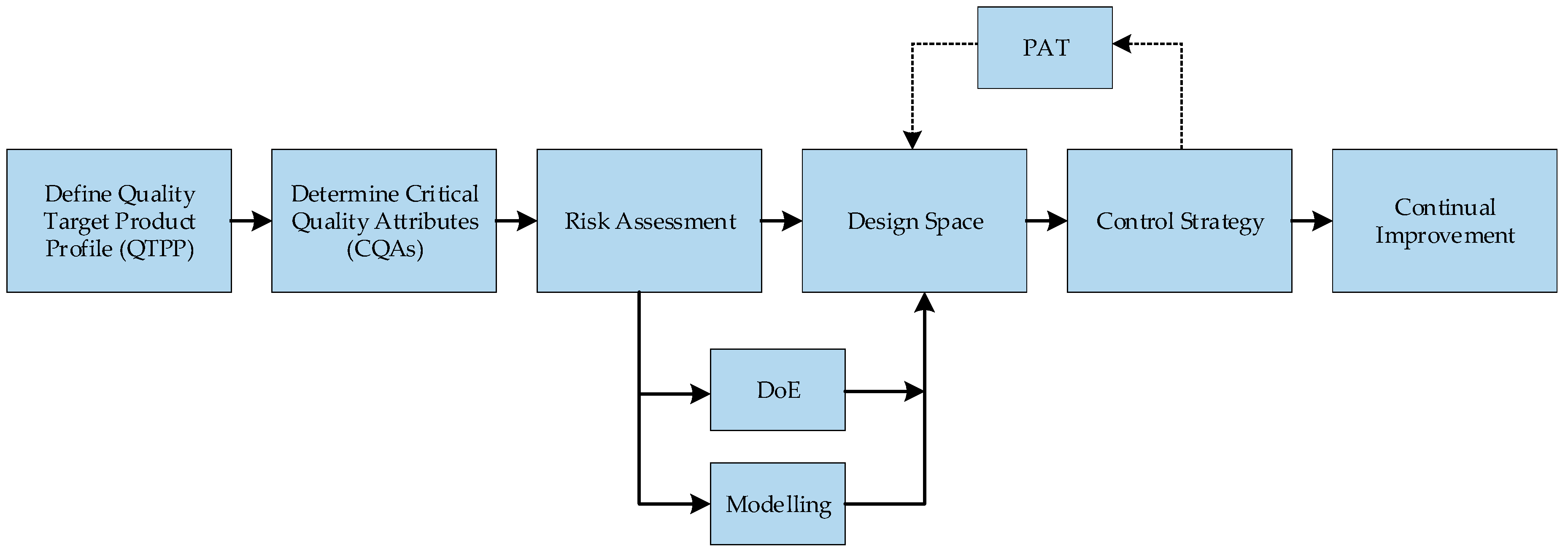
Despite the effort involved, complex models help to understand the basics of the considered process. In addition, a model can save time and money in process development and plant optimization. The physico-chemical model helps especially in the extraction of plant constituents, since the amount of target components in the used plant parts fluctuates due to natural influencing factors. With the help of a model, only a few preliminary tests have to be carried out in order to optimise the steam distillation. Modelling is also important for pharmaceutical products, since quality assurance is increasingly determined and by a quality by design (QbD) approach. Furthermore, regulatory agencies demand the demonstration of process understanding using digital twins of the manufacturing process. This development approach under QbD is represented in Figure 1. The main target of the QbD approach is to ensure product quality even under naturally occurring parameter fluctuations [12].

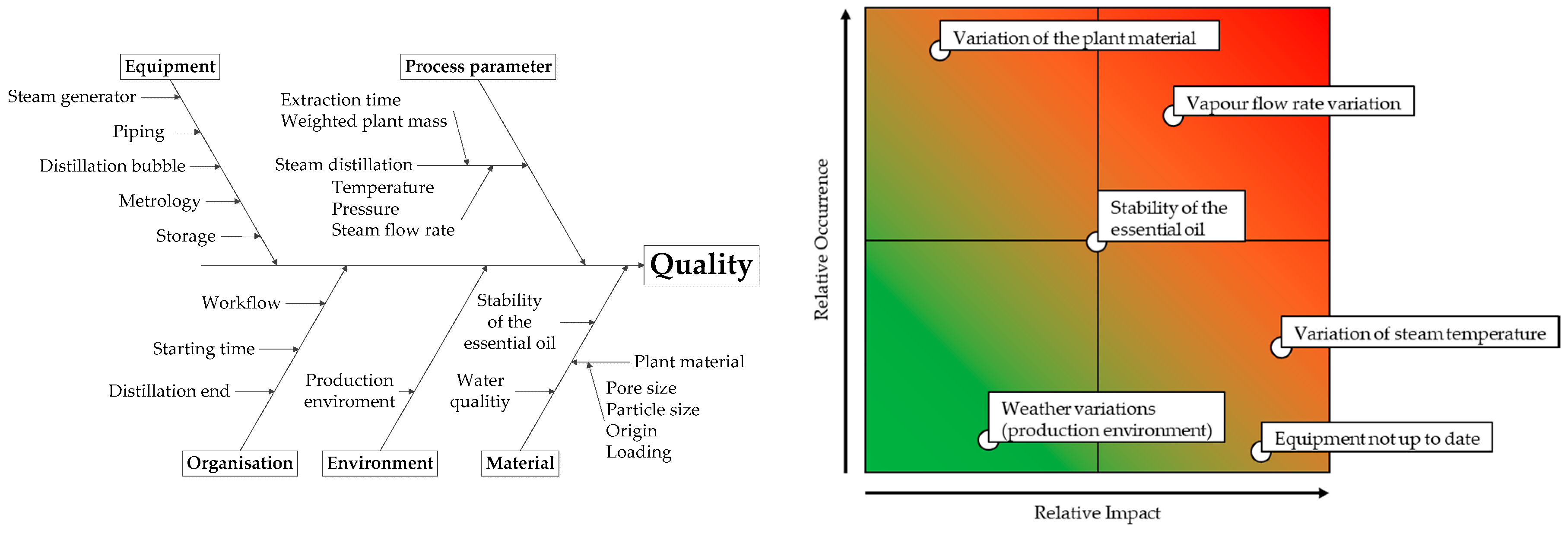
Before the start of model development, an initial risk assessment is necessary to appropriately define the modelling task, the necessary model depth and required variables. The risk assessment for steam distillation is shown in Figure 2 using an Ishikawa diagram.

An exemplary selection of parameters is visualised with a failure mode and effects analysis (FMEA), based on prior experience regarding rate of occurrence and relative impact on product quality of the respective risk. The derived scoring of all the FMEA considered variables is explained in

Table 1. QbD initial risk assessment: FMEA.

Risk	Impact	Occurrence	Comment
Equipment not up to date	9	1	Incidents due to material exhaustion. Well controlled through maintenance intervals and process control devices.
Stability of the essential oil	5	5	Essential oils are prone to oxidation under oxygen and light, which can be mitigated by the storage conditions.
Vapour flow rate variation	7	8	Start-up heating causes condensed water blocking fast diffusion of vapour. Vapour flow limited by packing back-pressure. Appropriate steam unit with process control.
Variation of steam temperature	9	3	The steam temperature varies depending on the column back pressure.
Variation of the plant material	2	9	Plant material properties like content, plant parts, particle size distribution and wettability are highly dependent on cultivation conditions, harvest and drying.
Weather variations (production environment)	3	1	Distillation equipment often is not sufficiently insulated.

.

The risk factors identified in this risk assessment have to be mitigated to achieve a solid control strategy and derive a design space, which provides consistent quality.

The tools to define this design space are experimental design of experiments (DoE) and physico-chemical modelling. A validated physico-chemical model enables better utilization of experimental data and can be used to characterise the design space, which results in a reduction of the required experiments [12].

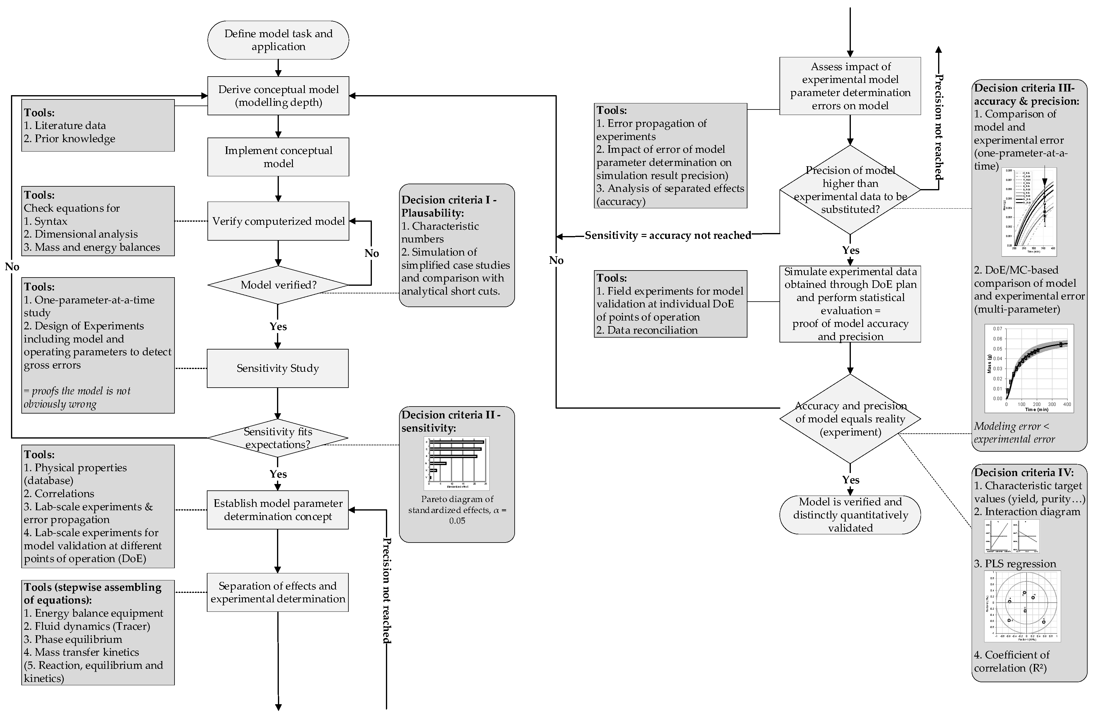
The model development in this paper follows the model development workflow from Sixt et al. [12], shown in Figure 3. This workflow ensures defined model quality, including experimental validation and statistical evaluation of accuracy and precision. The workflow is divided into four segments.

The first segment consists of model definition and implementation. Successful model implementation leads to a plausible model, which reacts appropriately to changing input parameters. Characteristic numbers describing mass and energy transfer and the mass balances can be reviewed to assess the correct implementation of the model equations.

The second segment gives conclusions to the model parameter sensitivity. The sensitivity is an important parameter during process development and model parameter determination, because the sensitivity reflects the influence of the considered parameters on simulation results. As second decision criteria, sensitivity studies are carried out. This includes one- and multi-parameter-at-a-time studies.

In the single parameter studies, only one parameter is changed while all other parameters are kept at the average value. The result of the performed simulations shows the influence of the changed variable. This study reveals errors in the developed model, because the influence of most input variables is known. The multi parameter studies are carried out to evaluate the influence of the variables in comparison to each other. Therefore, all parameters are changed within a DoE design. The obtained simulation results are evaluated with a statistical analysis tool. As a result, Pareto charts of standardised effects are generated. These Pareto charts give an overview of the significant parameters and thus improve process knowledge.

In the third segment the model parameter determination and the third decision criteria take place. For the model parameter determination, it is important to focus on the significant parameters from segment 2. Less significant parameters do not have to be measured with the highest precision. Overall, it is more important to separate the different effects of mass transfer, because the model parameters remain valid when process parameters change [14]. Afterwards model accuracy and precision are checked. Therefore, simulation results are compared with experimental results at a specific point. The experimental precision is obtained by repeated measurements. For repeated simulations with the same model parameters, the precision is close to 100%. However, the error of the model parameter determination must also be taken into account. If the model parameter of the repeated simulations is set to the minimum and maximum values, the precision of the simulation is determined.

The fourth segment helps to prove the model validation in the range of the DoE. For this purpose, field experiments are carried out at different points of the DoE and the achieved results are compared with a simulation with the corresponding process parameters.

After successfully completing all four segments, the developed physico-chemical model is verified and validated, and the model can be used for process development and optimisation.

Other models, which are verified and validated with this process model development workflow, summarised schematically in Figure 3, cover a solid–liquid (phyto-) extraction [12], upstream fermentation [15], liquid–liquid extraction [16], continuous single-pass tangential flow filtration [17], precipitation [18] and chromatography [19]. This demonstrates the benefit of a methodical approach to model development.

2. Modelling Steam Distillation

Before the model developed for this work is presented, an overview of already published models is given in

Table 2. Overview of modelling approaches.

Author and Year	Reference	Plant Material	Particle Shape	Essential Oil	Model	Mass Transport inside the Particle	Mass Transport into the Steam
Denny 1979	[23]	Lavandin	Glandular trichomes	Pseudo-single component	Crude model	Not considered	Energy supply is limited
Benyoussef 2002	[20]	Coriander fruits	Isotropic	Pseudo-single component	Diffusional model and model based on first order kinetics	Diffusion or diffusion with first order kinetic	Not considered
Koul 2003	[24]	Lemon grass	Chopped or unchopped	Pseudo-single component	First order kinetics	First order kinetics	Not considered
Cassel 2006	[22]	Lemon grass, twigs and leaves	One-dimensional rectangle geometry	Pseudo-single component	Diffusional model based on the Fick’s second law	Unsteady-state diffusion (Fick’s second law)	Not considered
Sovova 2006	[21]	Creeping thyme leaves/intact coriander fruits	Spherical/slab	Pseudo-single component	Broken and intact cells	First order kinetics or linear	Not considered
Sowbhagya 2007	[25]	Celery	Seeds	Pseudo-single component	First order kinetics	First order kinetics	Not considered
Cerpa 2008	[11]	Lavandin	Glandular trichomes	Individual oil components	Phenomenological model	First order kinetics	Vapour pressure is limiting
Milojevic 2008	[26]	Juniper berries	Isotropic	Pseudo-single component	Washing and diffusion	Unsteady-state diffusion (Fick’s second law)	Not considered
Sowbhagya 2007	[27]	Cumin	Seeds	Pseudo-single component	First order kinetics	First order kinetics	Not considered
Babu 2009	[28]	Eucalyptus foliage	Waxy thin layer	Pseudo-single component	Yields equals Langmuir equation	Not considered	Not considered
Cassel 2008	[23]	Rosemary, basil, lavender	One-dimensional rectangle geometry	Pseudo-single component	Diffusional model based on the Fick’s second law	Unsteady-state diffusion (Fick’s second law)	Not considered
Kapas 2011	[24]	Fennel seeds	Isotropic	Pseudo-single component	Washing and diffusion	Unsteady-state diffusion (Fick’s second law)	Not considered
Pornpunyapat 2011	[25]	Agarwood	Isotropic	Pseudo-single component	Washing and diffusion	Unsteady-state diffusion (Fick’s second law)	Not considered
Sartor 2011	[1]	Rosemary	-	Pseudo-single component	Ideal plug flow model	Not considered	Equilibrium coefficient is limiting
Xavier 2011	[26]	Asteraceae	Leaves/sticks	Pseudo-single component	Model of Sovova based on mass transfer fundamentals	Diffusion	Not considered
He 2016	[27]	Herbs	Sphere	Pseudo-single component	Diffusion model	Diffusion	Not considered
Pavicevic 2016	[28]	Juniper berry	Isotropic	Pseudo-single component	Washing and diffusion	First order kinetics	Not considered
Katiyar 2017	[29]	Menthol mint	One-dimensional rectangle geometry	Pseudo-single component	Diffusional model based on the Fick’s second law	Unsteady-state diffusion (Fick’s second law)	Not considered

comparing plant material, particle form, description of essential oil and mass transfer effects in steam and liquid phase. When comparing the 18 models, it can be seen that the model parameters are generally fitted to experimental results of steam distillations. For this reason, none of the models is predictive. In addition, 17 models use a pseudo-single component, so no distinction between different oil components is possible. Furthermore, most models assume that the evaporation of essential oil components is fast compared to diffusion in the particle. Evaporation is therefore neglected. For this reason, not all transport effects are taken into account in the corresponding models. Since none of the models developed so far meets the requirements for a predictive, physico-chemical model, a new model was developed for this project.

In the existing models, two model approaches were used for the plant extraction part.

• First order kinetic: The extraction of the essential oil from the plant particles is assumed to follow a first order kinetic. The composition of the essential oil in the plant particle remains constant [11,20].
• Diffusion: When the extraction of the essential oil is modelled with diffusion, Fick’s second law is solved for a sphere or a slab. Due to different extraction rates during steam distillation, the extraction is divided into washing and diffusion. Washing is realised by a high diffusion coefficient and takes place when broken plant cells are present. Diffusion occurs with plant cells and is slower due to the plant membrane [21,22].

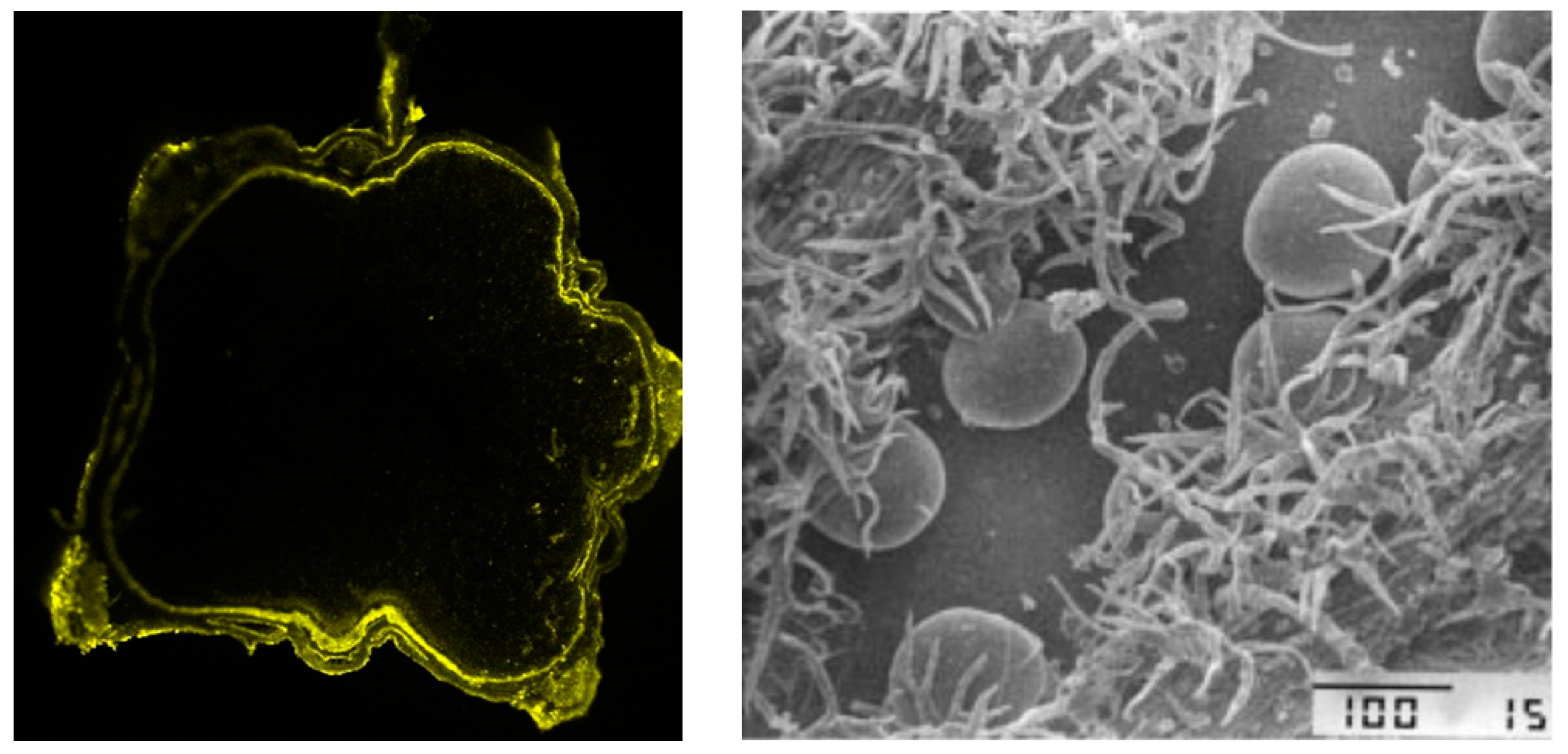
The models presented show that there are two possible ways that extraction mechanisms are described. This can also be seen in Figure 4 where different oil storage locations are shown. The essential oil of caraway is found in subcutaneous oil seams and needs to diffuse through the hard plant surface. In contrast to that, the essential oil of lavender is located in the surface near trichomes. These trichomes are in direct contact with the steam and release the essential oil as they break up.

2.1. Model Depth

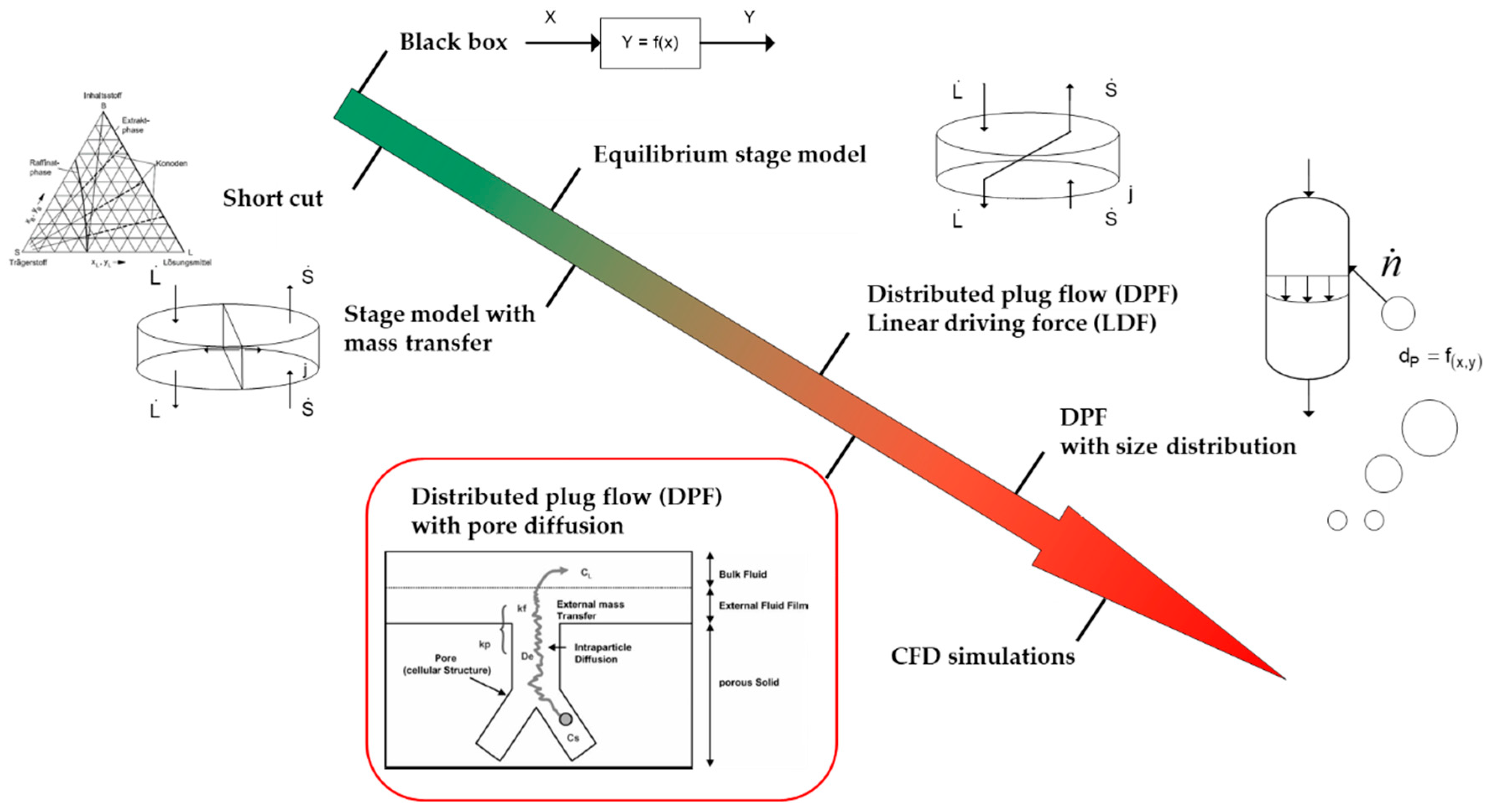
Different model depths are available, as shown in Figure 5. The least complex model is the black box model. In this model, there are only material flows that are linked to simple relationships. The model equations are based only on mass balance and empirical data. The most complex models are computational fluid dynamic (CFD) models. The focus of these models is to show the local behaviour of fluids flow patterns, which is not the dominant challenge in plant extraction [12,23,24].

It is important to choose a model depth which is suitable for solving the modelling task. If the model depth is set too low, complex material and energy transfer effects cannot be discerned. Consequently, the modelling task cannot be fulfilled properly. In contrast, a model depth that is too complex wastes time and resources. One of the reasons for this is that more complex model parameters have to be determined [25].

2.2. Modelling Objective Definition

A proper description of steam distillation for process development and scale-up manufacturing optimization requires a complex model, which allows the separation of mass transfer effects responsible for the extraction of essential oils from plant material. The natural variability of the origin of essential oil on the plant particle has to be considered, which can be achieved by a distributed plug flow model, including pore diffusion, and limited solubility of the target component in water as an extraction solvent.

2.3. Model Overview

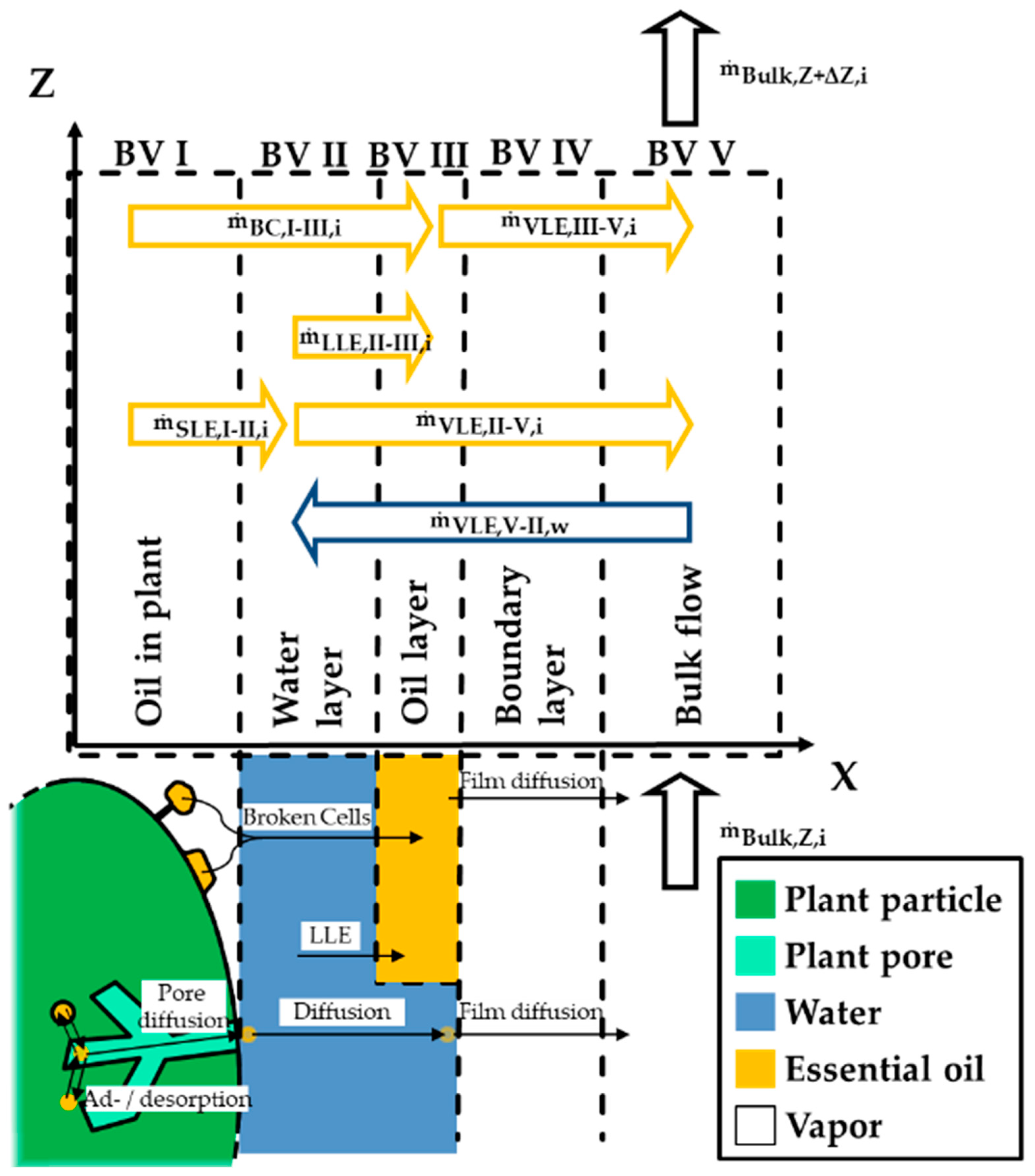
Figure 6 shows an overview of the developed model. It contains the cell disruption for “free” oil, liquid–liquid equilibrium, solid–liquid extraction for oil in plant particle and condensation of water.

2.4. Pore Diffusion Model

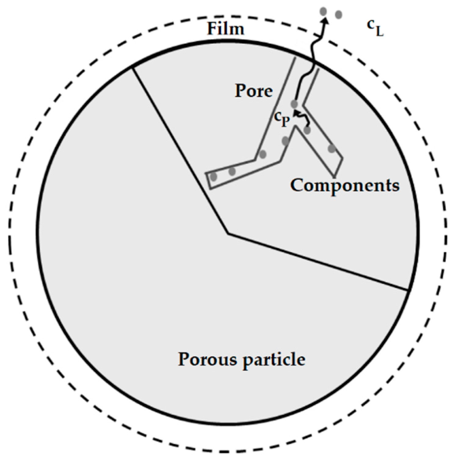
The pore diffusion model is used to describe the diffusion of the oil from the particle. It was originally developed for chromatography and is an extension of the diffusion model used in the literature. The expansion includes, as shown in Figure 7, the consideration of the plant particle porosity. Therefore, the pore diffusion model has a higher level of detail [12,27].

For spherical particles, Equation (1) is obtained using Fick’s second law for porous media. In the equation, ${\mathsf{\epsilon }}_{\mathrm{p}}$ is the porosity of the particle, $c_{p,i}\left(\mathrm{z},\mathrm{r},\mathrm{t}\right)$ is the concentration in the liquid phase, $q_i(\mathrm{z},\mathrm{r},\mathrm{t})$ is the concentration in the solid phase, r is the radius of the particle and $D_{eff,i}$ is the effective diffusion coefficient [12].

$${\mathsf{\epsilon }}_{\mathbf{p}}·\frac{\mathbf{\partial }{\mathbf{c}}_{\mathbf{p},\mathbf{i}}\left(\mathbf{z},\mathbf{r},\mathbf{t}\right)}{\mathbf{\partial }\mathbf{t}}+\left({\mathbf{1}-\mathsf{\epsilon }}_{\mathbf{p}}\right)·\frac{\mathbf{\partial }{\mathbf{q}}_{\mathbf{i}}(\mathbf{z},\mathbf{r},\mathbf{t})}{\mathbf{\partial }\mathbf{t}}=\frac{\mathbf{1}}{{\mathbf{r}}^{\mathbf{2}}}·\frac{\mathbf{\partial }\left({\mathbf{r}}^{\mathbf{2}}{·\mathbf{D}}_{\mathbf{eff},\mathbf{i}}·\frac{\mathbf{\partial }{\mathbf{c}}_{\mathbf{p},\mathbf{i}}\left(\mathbf{z},\mathbf{r},\mathbf{t}\right)}{\mathbf{\partial }\mathbf{r}}\right)}{\mathbf{\partial }\mathbf{r}}.$$

(1)

2.4.1. Boundary and Initial Conditions

In order to solve the derived second order differential equation, two boundary and one initial condition are required. A uniform loading of the plant particle is assumed as the initial condition. The mass balance at the particle edge is used as the first boundary condition. It is assumed that the mass diffusing from the particle is equal to the mass that is absorbed in the surrounding water layer. For the second boundary condition it is assumed that the concentration has a maximum in the middle of the particle. The second boundary condition is shown in Equation (2) [28].

$$\mathrm{r}=0, \frac{\partial {\mathrm{c}}_{\mathrm{p}}\left(\mathrm{z},\mathrm{r},\mathrm{t}\right)}{\partial \mathrm{r}}=0$$

(2)

2.4.2. Equilibrium

Within the plant pores there is a solid–liquid adsorption equilibrium. As is usual in chromatography, this equilibrium is described with an adsorption isotherm. The simplest example of an isotherm is the Henry isotherm (Equation (3)), which creates a linear relationship between the concentrations in the liquid phase and in the solid phase. The proportionality factor between concentration c and loading q is the Henry coefficient $K_H$ [12,29].

$$\mathrm{q}={\mathrm{K}}_{\mathrm{H}}·\mathrm{c}$$

(3)

An example for a first order isotherm is the Langmuir isotherm (Equation (4)). Like the Henry isotherm, it is linear at low concentrations. At high concentrations, the Langmuir isotherm approaches the maximum loading $q_{max}$. The Langmuir coefficient $K_L$ is the quotient of the adsorption and the desorption rate constant. In phytoextraction, there are usually no pure adsorption equilibria, since the target substances are often bundled in vacuoles. This is often corrected with a radial distribution of the components [29,30]. If this distribution is not known, the Langmuir isotherm can also be supplemented with a capacity factor a, which adjusts the isotherm to the uneven distribution in the particle [12].

$${\mathrm{q}=\mathrm{q}}_{\max }·\mathrm{a}·\frac{{\mathrm{K}}_{\mathrm{L}}·\mathrm{c}}{{1+\mathrm{K}}_{\mathrm{L}}·\mathrm{c}}$$

(4)

The Langmuir isotherm was expanded in 1938 by Brunauer, Emmett and Teller in the event of an existing saturation concentration of the target component in the liquid phase. The expanded isotherm is similar to the Langmuir isotherm for small concentrations, since only one layer is formed on the adsorption surface. When the concentration in the liquid approaches the saturation concentration, an infinite number of layers is formed. The modified isotherm is shown in Equation (5) [31].

$$\mathrm{q}=\frac{{\mathrm{K}·\mathrm{q}}_{\max }·\mathrm{c}}{\left({\mathrm{c}}_{\mathrm{sat}}-\mathrm{c}\right)·\left(1+\frac{\left(\mathrm{K}-1\right)·\mathrm{c}}{{\mathrm{c}}_{\mathrm{sat}}}\right)}$$

(5)

2.4.3. Water Layer

For the diffusion of the components through the water layer, as for the pore diffusion model, the second Fick’s law for the spherical shell (Equation (6)) is used again. In the equation, $D_{12,i}$ is the binary diffusion coefficient of the components in water.

$$\frac{\partial {\mathrm{c}}_{\mathrm{w},\mathrm{i}}\left(\mathrm{z},\mathrm{r},\mathrm{t}\right)}{\partial \mathrm{t}}=\frac{1}{{\mathrm{r}}^2}·\frac{\partial \left({\mathrm{r}}^2{·\mathrm{D}}_{12,\mathrm{i}}·\frac{\partial {\mathrm{c}}_{\mathrm{w}}\left(\mathrm{z},\mathrm{r},\mathrm{t}\right)}{\partial \mathrm{r}}\right)}{\partial \mathrm{r}}$$

(6)

2.5. Cell Disruption

If the essential oil is superficial, the plant hairs are destroyed by the steam. The released oil creates an oil layer floating on the water [11,32]. The number of destroyed trichomes and thus the released oil mass flow ${\dot{m}}_{BC,I-\mathit{III},i}(\mathrm{z},\mathrm{t})$ is described with a first order kinetic (Equation (7)).

$${\dot{\mathrm{m}}}_{\mathrm{BC},\mathrm{I}-\mathrm{III},\mathrm{i}}(\mathrm{z},\mathrm{t})=-\mathrm{k}\left(\mathrm{Y}\right)·{\mathrm{m}}_{\mathrm{BC},\mathrm{i}}(\mathrm{z},\mathrm{t})$$

(7)

The disruption rate k(T) is calculated using the Arrhenius equation, given in Equation (8), in order to simulate a temperature influence on the destruction of the plant hairs.

$$\mathrm{k}\left(\mathrm{T}\right){=\mathrm{k}}_0{·\mathrm{e}}^{-\frac{\mathrm{EA}}{\mathrm{R}·\mathrm{T}}}$$

(8)

where $k_0$ is the pre-exponential frequency factor, EA is the activation energy, R is the universal gas constant and T is the temperature.

2.6. Vapour–Liquid Equilibrium

The mass transport ${\dot{m}}_{VLE,\mathit{II}/\mathit{III}-V,i}(\mathrm{z},\mathrm{t})$ from the water or oil layer into the gas phase is shown in Equation (9).

$${\dot{\mathrm{m}}}_{\mathrm{VLE},\mathrm{II}/\mathrm{III}-\mathrm{V},\mathrm{i}}(\mathrm{z},\mathrm{t})={\mathrm{k}}_{\mathrm{vap}}·\mathrm{A}(\mathrm{z},\mathrm{t})·({\mathrm{c}}_{\mathrm{V},\mathrm{i}}(\mathrm{z},\mathrm{t})-{\mathrm{c}}_{\mathrm{V},\mathrm{eq},\mathrm{i}}(\mathrm{z},\mathrm{t}))$$

(9)

where ${\mathrm{k}}_{\mathrm{vap}}$ is the rate constant of the evaporation, $\mathrm{A}\left(\mathrm{z},\mathrm{t}\right)$ is the surface of the respective phase, $c_{V,i}\left(\mathrm{z},\mathrm{t}\right)$ is the current concentration in the gas phase and $c_{V,eq,i}\left(\mathrm{z},\mathrm{t}\right)$ is the equilibrium concentration in the gas phase. The surface area of the essential oil is calculated with the volume $\mathrm{V}(\mathrm{z},\mathrm{t})$ and the height of the oil layer (Equation (10)).

$${\mathrm{A}}_{\mathrm{eo}}\left(\mathrm{z},\mathrm{t}\right)=\frac{\mathrm{V}(\mathrm{z},\mathrm{t})}{\mathrm{h}}$$

(10)

The surface area of the water phase is calculated using the surface area of the plant particle. The surface area of the essential oil is subtracted from the total area. The equilibrium concentration in the gas phase is calculated for both phases separately. The equilibrium concentration of free oil is based on Raoult’s law (Equation (11)).

$${\mathrm{c}}_{\mathrm{V},\mathrm{eq},\mathrm{i}}\left(\mathrm{z},\mathrm{t}\right)=\frac{{\mathrm{x}}_{\mathrm{o},\mathrm{i}}\left(\mathrm{z},\mathrm{t}\right){·\mathrm{p}}_{\mathrm{i}}^0}{\mathrm{R}·\mathrm{T}}$$

(11)

where $x_{o,i}\left(\mathrm{z},\mathrm{t}\right)$ is the molar mass fraction of the component in the oil phase and $p_i^0$ is the vapour pressure of the pure substance. The equilibrium concentration over the water phase is described using the activity $a_i\left(\mathrm{z},\mathrm{t}\right)$ of the oil components and the mass fraction in the water phase $x_{w,i}\left(\mathrm{z},\mathrm{t}\right)$ (Equation (12)).

$${\mathrm{c}}_{\mathrm{V},\mathrm{eq},\mathrm{i}}\left(\mathrm{z},\mathrm{t}\right)=\frac{{\mathrm{a}}_{\mathrm{i}}\left(\mathrm{z},\mathrm{t}\right){·\mathrm{x}}_{\mathrm{w},\mathrm{i}}\left(\mathrm{z},\mathrm{t}\right){·\mathrm{p}}_{\mathrm{i}}^0}{\mathrm{R}·\mathrm{T}}$$

(12)

2.7. Liquid–Liquid Equilibrium

The mass transport ${\dot{m}}_{LLE,\mathit{II}-\mathit{III},i}(\mathrm{z},\mathrm{t})$ from the oil phase into the liquid film is calculated using Equation (13).

$${\dot{\mathrm{m}}}_{\mathrm{LLE},\mathrm{II}-\mathrm{III},\mathrm{i}}(\mathrm{z},\mathrm{t})={\mathrm{k}}_{\mathrm{LLE},\mathrm{i}}·\mathrm{A}(\mathrm{z},\mathrm{t})·\left({\mathrm{c}}_{\mathrm{w},\mathrm{i}}(\mathrm{z},\mathrm{t})-{\mathrm{c}}_{\mathrm{w},\mathrm{eq},\mathrm{i}}(\mathrm{z},\mathrm{t})\right)$$

(13)

where $k_{LLE,i}$ is the rate constant of the liquid–liquid extraction, $\mathrm{A}\left(\mathrm{z},\mathrm{t}\right)$ is the surface area of the essential oil, ${\mathrm{c}}_{\mathrm{w},\mathrm{i}}\left(\mathrm{z},\mathrm{t}\right)$ is the concentration of the surrounding water and $c_{w,eq,i}\left(\mathrm{z},\mathrm{t}\right)$ is the equilibrium concentration in the aqueous phase and can be calculated using the equilibrium constant $K_{LLE,i}$ (Equation (14)).

$${\mathrm{c}}_{\mathrm{w},\mathrm{eq},\mathrm{i}}\left(\mathrm{z},\mathrm{t}\right){=\mathrm{K}}_{\mathrm{LLE},\mathrm{i}}{·\mathrm{c}}_{\mathrm{eo},\mathrm{i}}(\mathrm{z},\mathrm{t})$$

(14)

where $c_{eo,i}(\mathrm{z},\mathrm{t})$ is the concentration of the component in the oil phase.

2.8. Distributed Plug Flow (DPF) Model

The distributed plug flow model was derived by Danckwerts for chromatography in 1952. It characterises the macroscopic mass transport of the target components in the gas phase (Equation (15)) [33,34,35].

$$\begin{array}{c}\frac{\partial {\mathrm{c}}_{\mathrm{V},\mathrm{i}}(\mathrm{z},\mathrm{t})}{\partial \mathrm{t}}{=\mathrm{D}}_{\mathrm{ax}}·\frac{{\partial }^2{\mathrm{c}}_{\mathrm{V},\mathrm{i}}(\mathrm{z},\mathrm{t})}{\partial {\mathrm{z}}^2}-\frac{\mathrm{u}}{\mathsf{\epsilon }}·\frac{\partial {\mathrm{c}}_{\mathrm{V},\mathrm{i}}\left(\mathrm{z},\mathrm{t}\right)}{\partial \mathrm{z}}\\ -\frac{1-\mathsf{\epsilon }}{\mathsf{\epsilon }}{·\mathrm{k}}_{\mathrm{vap}}·\frac{6}{{2·\mathrm{r}}_{\mathrm{p}}+2·\mathsf{\delta }\mathrm{r}}·\left(1-\frac{\mathrm{A}(\mathrm{z},\mathrm{t})}{{\mathrm{A}}_{\mathrm{tot}}}\right)·\left[{\mathrm{c}}_{\mathrm{V},\mathrm{i}}\left(\mathrm{z},\mathrm{t}\right){-\mathrm{c}}_{\mathrm{V},\mathrm{eq},\mathrm{i}}\left(\mathrm{z},\mathrm{t}\right)\right]\\ -\frac{1-\mathsf{\epsilon }}{\mathsf{\epsilon }}{·\mathrm{k}}_{\mathrm{vap}}·\frac{6}{{2·\mathrm{r}}_{\mathrm{p}}+2·\mathsf{\delta }\mathrm{r}}·\left(\frac{\mathrm{A}(\mathrm{z},\mathrm{t})}{{\mathrm{A}}_{\mathrm{tot}}}\right)·\left[{\mathrm{c}}_{\mathrm{V},\mathrm{i}}\left(\mathrm{z},\mathrm{t}\right){-\mathrm{c}}_{\mathrm{V},\mathrm{eq},\mathrm{i}}\left(\mathrm{z},\mathrm{t}\right)\right]\end{array}$$

(15)

The left side of the equation expresses the accumulation of the target substance. The terms for convection, dispersion and mass transfer can be found on the right. In the equation, $c_{V,i}(\mathrm{z},\mathrm{t})$ is the concentration in the gas phase, $D_{ax}$ is the axial dispersion coefficient, u is the gas velocity in an empty column, $\mathsf{\epsilon }$ is the bed porosity, $k_{vap}$ is the rate constant of the evaporation, $r_p$ is the plant particle radius, $\mathsf{\delta }r$ is the height of the surrounding water layer, $\mathrm{A}(\mathrm{z},\mathrm{t})$ is the surface area of the oil layer, ${\mathrm{A}}_{\mathrm{tot}}$ is the total surface of the particle with surrounding water layer and $c_{V,eq,i}\left(\mathrm{z},\mathrm{t}\right)$ is the equilibrium gas phase concentration.

Since there are no plant particles outside the distillation bubble and therefore there is little axial dispersion, the closed vessel boundary condition is assumed [33,34].

3. Materials and Methods

3.1. Plant Materials and Solvents

Dried caraway fruits from Elsbeth Müller (Lonnerstadt, Germany) and chopped, dried lavender flowers from Senger Naturrohstoffe (Dransfeld, Germany) were used as plant material. Caraway oil was obtained from v03 trading (Willich, Germany) and lavender oil from Primavera Life (Sulzberg, Germany). The analysis standards were prepared with camphor with a purity of 95 %, D-carvone with a purity of 96% and linalyl acetate with a purity of 97% from Sigma Aldrich (Steinheim, Germany) and D-limonene with a purity of 97% and linalool with a purity of 97% from Alfa Aesar (Kandel, Germany). Isopropanol (analytical) from VWR (Radnor, PA, USA) and acetone (analytical) from Sigma Aldrich (Steinheim, Germany) were used for the experiments.

For gas chromatography, hydrogen and nitrogen from Linde (Dublin, Ireland) were used.

3.2. Instruments and Devices

The percolation system consists of a LaPrep^® P130 pump from VWR (Radnor, PA, USA) and a steel column with a length of 10 cm and a diameter of 1 cm.

The maceration and shaking tests were carried out with the MKR 13 thermal shaker from HLC Biotech (Bovenden, Germany). The thermal shaker has an attachment for 50 mL centrifuge vials from VWR (Radnor, PA, USA) and for 2 mL Safe Lock Tubes from Eppendorf (Hamburg, Germany).

For steam distillation in lab scale, a glass apparatus consisting of a two-necked flask (volume: 1 L), a column (diameter: 2.6 cm; height 8.5 cm) containing the plant bed and a Liebig condenser (length: 25 cm, 4 °C water temperature) were used. The essential oil was collected and separated in 50 mL centrifuge vials from VWR (Radnor, PA, USA). A heating element (1.25 mL/min; 3 mL/min; 7.25 mL/min) was used to evaporate the water. A LaPrep^® P130 pump from VWR (Radnor, PA, USA) was used to keep the water level in the two-necked flask constant.

3.3. Analytics

A Scion 436 gas chromatograph from Bruker (Billerica, MA, USA) was used to carry out the analytics. A DB-5 column from Agilent (Santa Clara, CA, USA) with a length of 30 m and a diameter of 320 μm was used to separate the components.

To analyse caraway samples, the injection area was heated to 200 °C. The column oven was heated from 80 °C to 200 °C at a rate of 8 °C/min. The start and end temperature were held for 3 min each. The method therefore had a run time of 21 min. The detector was kept constant at 220 °C. Hydrogen was used as the carrier gas. The pressure at the column entrance was kept at 0.69 bar.

To analyse lavender samples, the injection area was heated to 250 °C. The column oven was first heated from 70 °C to 120 °C at a rate of 5 °C/min and then to 200 °C at a rate of 15 °C/min. The start and end temperature were held for 5 min each, and the temperature of 120 °C was held for 2 min. This resulted in a run time of 27.33 min. The detector was kept constant at 250 °C. Again, hydrogen was used as the carrier gas. The volume flow through the column was set to 1.5 mL/min.

In both methods, 1 µL of the sample was injected with a split of 120 or 30, depending on the expected concentration. To ensure that the essential oil did not separate from the water phase, the samples were diluted 1:1 with isopropanol.

The coefficients of determination (R²) for the calibration curves were 0.999 for D-carvone and D-limonene, while linalyl acetate and linalool showed R² of 0.995 and 0.997, respectively.

3.4. Model Parameter Determination

To determine the total content of the caraway, percolation of 2 g caraway was carried out at room temperature. A mixture (in volume) of 70% acetone and 30% water with 1 mL/min flowed through the percolation column until no target components were detected (6–8 h).

The total content of the lavender was determined using steam distillation, since the oil-bearing plant hairs were not completely destroyed during percolation. Then, 5.4 g of the lavender flowers were poured into the steam distillation column. The heating element evaporated 1.25 mL water per minute, supplying a vapour load of 238.9 m³/m² h saturated steam until no target components could be detected (1 h).

To determine the solid–liquid isotherms, caraway and lavender were placed in a 50 mL centrifuge vial and mixed with water. The samples were then brought to 99 °C in the thermal shaker. After equilibrium was reached, a sample was taken from the water phase and analysed. For caraway, 0.06 g, 1 g, 1.75 g, 1 g, 1.75 g, 3 g, 3 g and 3 g were mixed with 42 g, 25 g, 25 g, 15 g, 15 g, 25 g, 15 g and 15 g water. For lavender, 0.04 g, 0.75 g, 1.78 g, 2 g, 2.5 g and 3 g were mixed with 45 g, 41 g, 37 g, 33 g, 30 g and 33 g water.

To determine the liquid–liquid equilibrium, equilibrium tests were carried out at room temperature and in the thermal shaker at 99 °C. For the experiment, 0.5 mL of the purchased essential oil was mixed with 0.5 mL or with 1.5 mL water and poured into a 2 mL Safe Lock Tube. The mixture was then brought into equilibrium and a sample of both phases was taken. In addition, tests of equilibrium with essential oil from the first 15 min of a previously carried out steam distillation were determined. Since the oil phase was hardly visible on the collected water, the sample was diluted with 15 mL isopropanol to create a single-phase mixture. A sample was taken from this mixture to determine the second required concentration.

Vapour liquid equilibrium was calculated using Non-Random-Two-Liquid (NRTL) in Aspen Properties^® from AspenTech (Bredford, MA, USA) and compared to literature data.

3.5. Experimental Validation Runs

For the validation, a statistical test plan (DoE) for caraway and lavender was created with two influencing factors and a centre point. The centre point test was carried out twice.

In the caraway DoE, the steam flow rate and the accessibility of the essential oil varied, as summarised in

Table 3. Summary of experimental parameters.

Parameter DoE	Condensate Flowrate	Crushed Material	Extracted Material
Caraway	1/3/7 mL/min	0%/50%/100%	20 g
Lavender	1/3/7 mL/min	/	1.8/3.6/5.4 g

. The steam flow rate was regulated via the three levels of the heating element. To vary the accessibility of the essential oil, the caraway was squeezed with a steel roll for one minute. All, half or no caraway fruits were squeezed, to vary the fraction of broken seeds. For all experiments in the DoE, 20 g caraway seeds were weighed in.

In the lavender DoE, the amount of lavender varied in addition to the steam flow rate. For the DoE, 1.8 g, 3.6 g and 5.4 g lavender were weighed out.

The distillate stream was collected fractionally for 120 min. The sample collection vessel was changed every 4 min at a flow rate of 1300 m³/m²·h. At the lower gas loads, the sample vessel was changed every 5 min. To collect the entire extracted mass of essential oil, the samples were diluted 1:1 with isopropanol. This ensures that no film of essential oil floats on the water phase.

This represents a production environment quite in line with gas velocities around 0.07–0.4 m/s.

4. Model Parameter Determination

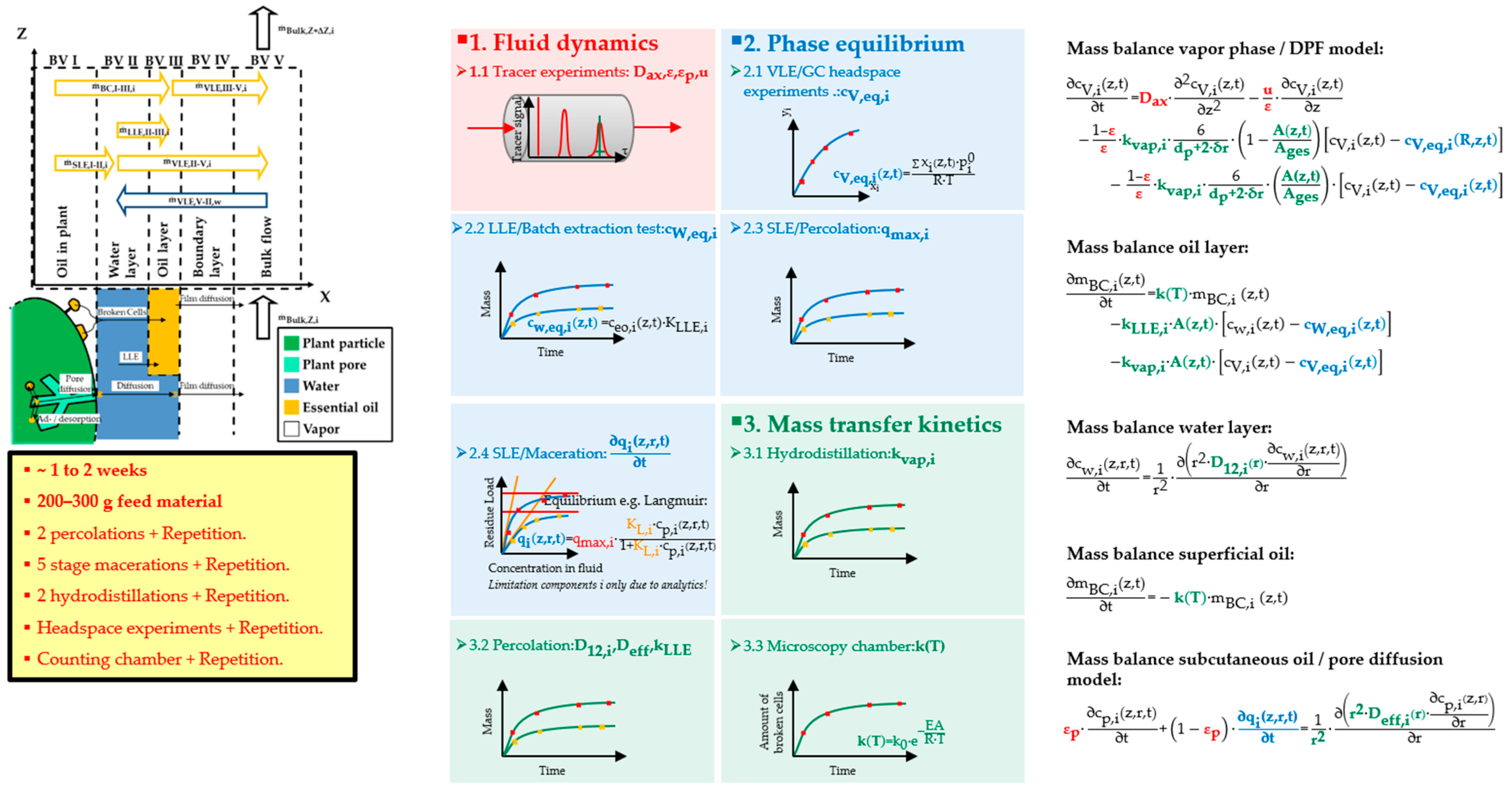
Any model parameter determination concept needs to be efficient and miniaturised due to time, manpower and test amounts needed in order to generate any physico-chemical process model of industrial project use. In this chapter, the required model parameters are highlighted, and a consistent model parameter determination concept is explained (Figure 8). The model parameters are divided into groups: fluid dynamics (red), equilibrium (blue) and mass transport kinetics (green). Overall, it takes any experienced team one to two weeks and 200 to 300 g of the plant material to carry out this model parameter determination concept.

4.1. Fluid Dynamics

Parameter of fluid dynamics are required to describe the behaviour of the gas phase and the backmixing of the target components in the gas phase. The axial dispersion, the porosity of the bed, the porosity of the individual particles and the velocity of the gas are the required parameters. To determine these parameters, tracer experiments can be executed. A tracer pulse is injected with a constant gas flow. How long the pulse took to pass through the column is measured at the column exit. In addition, the shape of the emerging peak is analysed in order to draw conclusions on the axial dispersion.

Alternatively, the axial dispersion coefficient $D_{ax}$ can be calculated using a correlation from Levenspiel (Equation (16)) [34].

$${\mathrm{D}}_{\mathrm{ax}}=\frac{{\mathrm{r}}_{\mathrm{p}}·\mathrm{u}}{{\mathsf{\epsilon }}^2·{\mathrm{A}}_{\mathrm{Column}}}$$

(16)

with ${\mathrm{r}}_{\mathrm{p}}$ is the particle radius, u is the gas velocity in an empty column, $\mathsf{\epsilon }$ is the bed porosity and ${\mathrm{A}}_{\mathrm{Column}}$ is the column cross section.

4.2. Phase Equilibria: Solid–Liquid, Liquid–Liquid and Liquid–Vapour

Since a thermodynamic system tends towards the equilibrium state, this state must be determined to describe the system. In the developed model different equilibrium conditions (i.e., vapour–liquid equilibrium, liquid–liquid equilibrium and solid–liquid equilibrium) need to be implemented to adequately model the steam distillation process.

The vapour–liquid equilibrium can be determined from the vapour pressures of the pure substances. If the accuracy is too low due to non-idealities, alternative headspace experiments can be carried out to determine the equilibrium curves. The activity and the partial pressure can be calculated from these equilibrium curves.

In order to determine the liquid–liquid equilibrium, shaking tests are necessary. The distribution coefficient of the components can be determined from the measured equilibrium line.

The solid–liquid equilibrium has to be determined for each plant system, since the composition of the essential oil can differ widely. To determine the equilibrium, the total content of the components in the considered plant parts is measured first. For this, percolation of the plant material is carried out. To determine the balance, macerations are then carried out with plant material and water. The concentration in the solid phase is determined either via the mass balance in the particles or by percolation with an acetone–water mixture. The observed isothermal parameters are calculated with the data points of the maceration tests. The maximum solubility in water required for the isotherm derived by Brunauer can be determined from the experiments on liquid–liquid equilibrium.

4.3. Mass Transfer Coefficients

Mass transport coefficients are required to describe the velocity of the components in the system. Evaporation kinetics, diffusion kinetics and cell opening kinetics are desired.

The evaporation kinetics can be determined using steam distillation. For this purpose, the volume flow emerging from the distillation is analysed with regard to the amount of essential oil. The evaporation kinetics are determined using the other known parameters. Optionally, the kinetics can also be estimated using a correlation. For this, a mass transfer factor $j_D$ is first calculated (Equation (17)) [36,37].

$${\mathrm{j}}_{\mathrm{D}}=\frac{0.499}{\mathsf{\epsilon }·{\mathrm{Re}}^{0.382}}$$

(17)

where ε is the porosity of the bed and Re is the Reynolds number. The Reynolds number is calculated using the particle radius $r_p$, the gas velocity in the empty column u, the gas density $\mathsf{\rho }$ and the viscosity μ of the gas (Equation (18)) [34].

$$\mathrm{Re}=\frac{{2·\mathrm{r}}_{\mathrm{p}}·\mathrm{u}·\mathsf{\rho }}{\mathsf{\mu }}$$

(18)

The rate constant $k_{vap}$ can be calculated from the mass transfer factor using Equation (19) [38].

$${\mathrm{j}}_{\mathrm{D}}=\frac{{\mathrm{k}}_{\mathrm{vap}}}{\mathrm{u}}·{\mathrm{Sc}}^{\frac{2}{3}}$$

(19)

where u is the velocity in an empty column and Sc is the Schmidt number. If the Reynolds number is greater than 2.5, then the Schmidt number of gases is approximately 1 [34].

The diffusion coefficients are determined by percolation with water. For this, the content of essential oil in the product stream is measured. The diffusion coefficients can be determined with a known solid–liquid equilibrium. Alternatively, the coefficients can be calculated using correlations. The binary diffusion coefficient $D_{12}$ is first calculated according to Wilke and Chang (Equation (20)) [39,40].

$${\mathrm{D}}_{12}=1.173·{10}^{-13}·\frac{{\left(2.26{·\mathrm{M}}_2\right)}^{0.5}·\mathrm{T}}{{\mathsf{\mu }}_2·{\mathsf{\upsilon }}_1^{0.6}}$$

(20)

where $M_2$ is the molar mass of the solvent, T is the temperature, ${\mathsf{\mu }}_2$ is the viscosity of the solvent and ${\mathsf{\upsilon }}_1$ is the molar volume of the target component at the boiling point of the pure substance. The effective diffusion coefficient $D_{eff}$ in a porous particle can be derived from the binary diffusion coefficient $D_{12}$ using a further correlation (Equation (21)) [27].

$${\mathrm{D}}_{\mathrm{eff}}=\frac{{\mathrm{D}}_{12}{·\mathsf{\epsilon }}_{\mathrm{p}}·\mathsf{\delta }}{\mathsf{\tau }}$$

(21)

where ${\mathsf{\epsilon }}_{\mathrm{p}}$ is the porosity of the particle, δ is the constrictivity factor and τ is the tortuosity factor. The tortuosity factor can also be determined using the porosity (Equation (22)) [27].

$$\mathsf{\tau }=\frac{{2-\mathsf{\epsilon }}_{\mathrm{p}}}{{\mathsf{\epsilon }}_{\mathrm{p}}}$$

(22)

Finally, the cell opening kinetics are determined. First the plant material is analysed with a microscope for the number of oil-carrying vessels. The plant material used is then purged with hot steam. Then it is examined again with a microscope to determine the number of destroyed vessels. The cell opening kinetics can be calculated from the number of destroyed vessels and exposure time.

5. Results

5.1. Model Verification

A plausibility study is carried out for model verification. It is checked whether the occurring variables have physically meaningful values. The results of the developed model show that there are no obvious errors in the implementation. Another verification step is the comparison of key figures with literature values. This is done in Section 5.3 together with the assessment of the model parameters.

5.2. Sensitivity Analysis

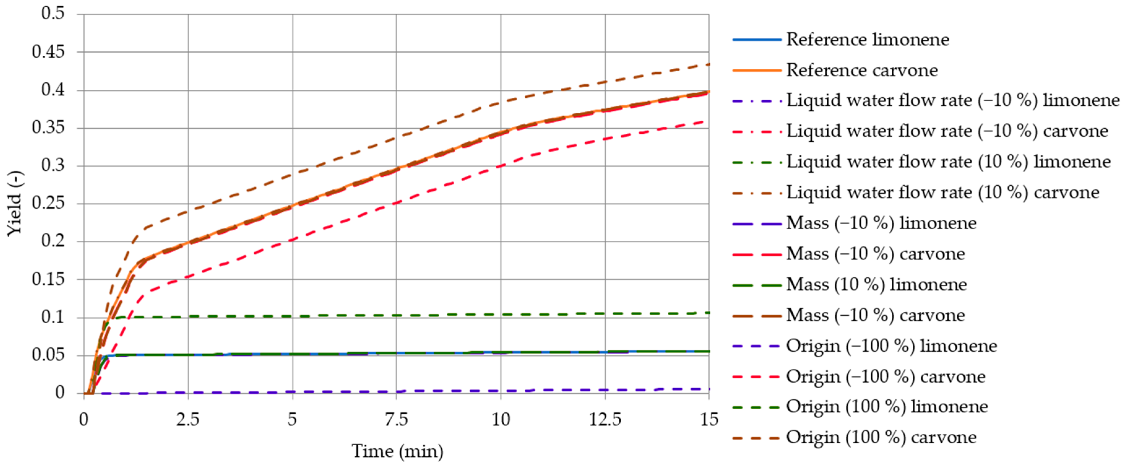
At the beginning of the sensitivity analysis, it is checked again whether there are obvious errors. For this purpose, a one-parameter-at-a-time study is carried out. Figure 9 displays the three variables with the greatest influence on the model yield. The main impact can be observed for the origin of the essential oil, while mass and liquid flow rate do not cause significant deviations from the reference. A closer look at the results shows that the model provides a rational change for each parameter variation. Again, no obvious error can be identified.

In the second part of the sensitivity analysis, the statistical significance of the parameters is calculated in order to obtain a model-based weighting of the influence of parameter fluctuations. The model and process parameters, shown in

Table 4. Considered range and influence of model parameters for the Pareto diagram. SLE: solid–liquid extraction; LLE: liquid–liquid extraction.

Model Parameter	Unit	Design Range	Influence Yield
Liquid water flow rate	(mL/min)	1–7	Moderate
Origin	(-)	0–1	High
Effective diffusion coefficient	(cm2/s)	${6 \times 10}^7{–6 \times 10}^5$	High
Breakup rate	(1/min)	0.01–0.5	High
Vapour pressure	(bar)	0.01–0.2	Moderate
Saturation concentration SLE	(g/L)	0.01–10	High
Equilibrium constant SLE	(-)	100–1000	Low
Maximum monolayer loading SLE	(g/L)	0.0001–0.05	Low
Bed porosity	(-)	0.3–0.5	Moderate
Particle porosity	(-)	0.5–0.7	Low
Loading	(g/L)	5–30	Moderate
Mass transport coefficient LLE	(cm/s)	90–110	Low
Equilibrium constant LLE	(-)	0.01–0.001	Low
Mean particle radius	(cm)	0.1–0.2	Moderate

, are used for the required (one component) test plan. The limits of the variables that include the expected values are also listed. The result of the simulation is considered to be the yield at 5 min, since the aim of the water and steam distillation is the efficient leaching out of the plant material. Since the full factorial design has $2^{13}$ simulation points and thus goes beyond the calculation framework, only a partial design plan is used. The higher order effects are neglected and only the information on the main effects are collected.

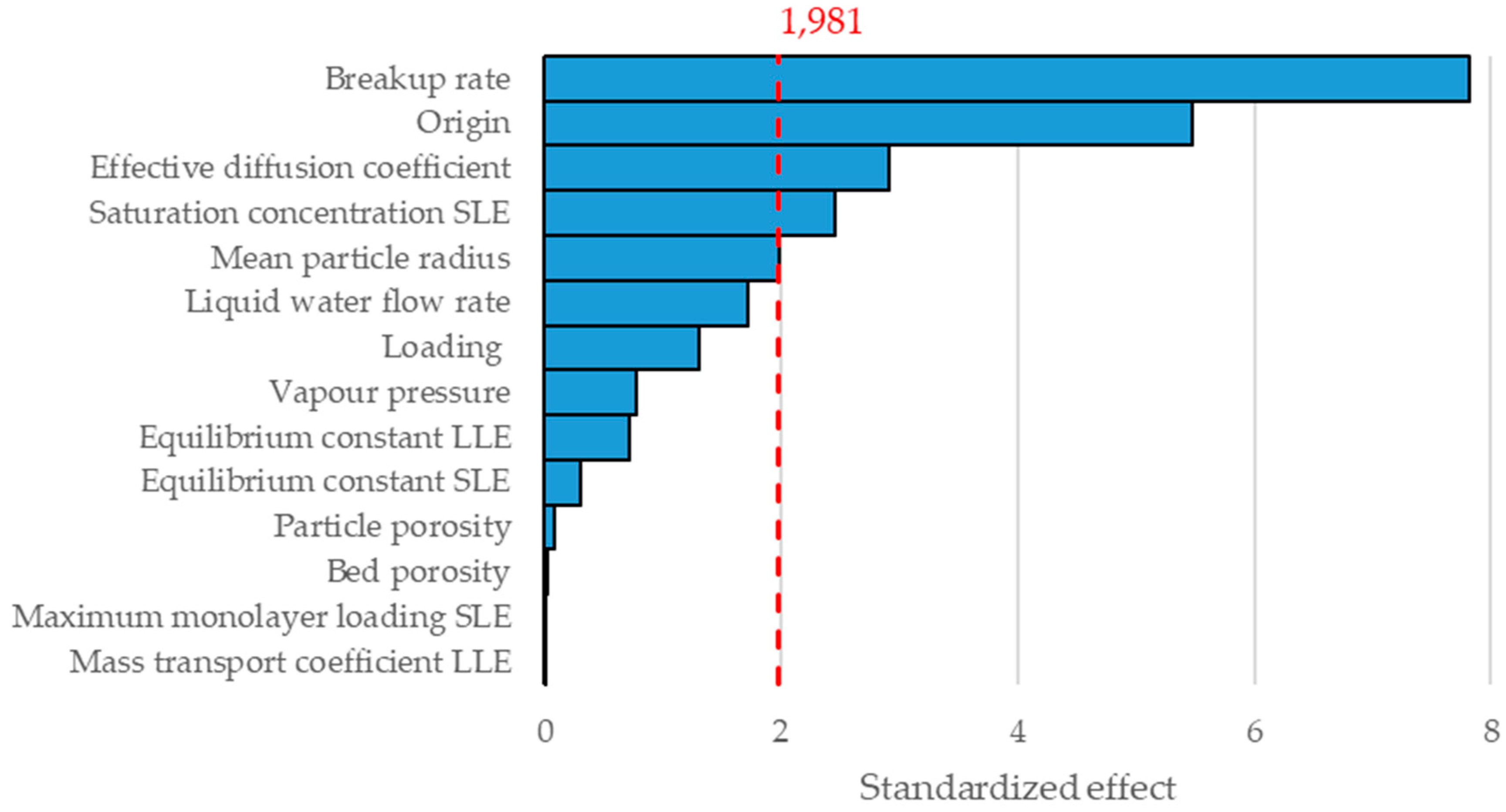
The Pareto chart of the determined, standardised effects for the yield at 5 min is shown in Figure 10.

In the Pareto diagram it can be seen that the breakup rate, origin, effective diffusion coefficient, saturation concentration in the solid–liquid extraction (SLE) and the mean particle radius are significant. These results also make sense, since steam distillation mainly depends on the mass transfer processes in the plant material.

5.3. Model Parameter Determination

As in Section 4 (model parameter determination), first the fluid dynamics parameters, then the equilibrium parameters and then the mass transport kinetics are discussed.

5.3.1. Fluid Dynamics

To determine the fluid dynamics parameters, the particle bed in the distillation column is first characterised. A particle size distribution of the caraway fruits and the lavender flowers is recorded, and the volume of the particles is converted into spheres. The caraway spheres calculated in this way have a radius of 0.1 ± 0.03 cm and those of lavender have a radius of 0.15 ± 0.04 cm. The bulk density of a caraway fill is 450 g/L [41] and the bulk density of a lavender fill is 100 g/L. The porosity of both fillings is set to 0.4.

The axial dispersion is calculated using the parameters of the particle bed, the correlation of Levenspiel (Equation (16)) and the velocity of the gas in the bed. For an experiment with a liquid volume flow of 3 mL/min, an axial dispersion coefficient of 9.3 ${\times 10}^{-4}$ ${\mathrm{m}}^2$/s results for the caraway bed and an axial dispersion coefficient of 1.4 ${\times 10}^{-3}$ ${\mathrm{m}}^2$/s results for the lavender bed. Since the axial dispersion coefficients are small, there is approximately an ideal piston flow [34]. The ideal piston flow is also assumed, for example, in the model developed by Sartor et al. [1]. This shows that the dispersion coefficient is of the right order. The Reynolds number is 36. Since the Reynolds number is greater than 0.2, there is a turbulent flow [42]. The Péclet number is not considered further, since the mass transport in the particle only takes place via diffusion. Advection prevails in the steam flow, as the axial dispersion coefficient shows.

5.3.2. Phase Equilibria: Solid–Liquid, Liquid–Liquid, Vapour–Liquid

To describe the equilibria, the total content is first determined. The total content of limonene in the caraway fruits is 9.1 ± 0.3 mg/${\mathrm{g}}_{\mathrm{TM}}$. The total content of carvone is 21.6 ± 0.7 mg/${\mathrm{g}}_{\mathrm{TM}}$. The caraway fruits therefore have 3% essential oil with a ratio of 70% carvone and 30% limonene.

Since a few hundred components may be present in lavender flowers, an external analysis of the first 5 min of steam distillation is carried out using GC-MS before the total content is determined. In the analysis, 43 different components are detected. The main components present in the lavender sample are camphor (27.22%), linalool (16.14%), myrcene (6.67%), cis-linalool oxide (6.26%), α-pinene (6.15%), 1,8-cineole (6.08%), borneol (5.66%), and trans-linalool oxide (5.66%). The further model validation and model parameter determination in this work is carried out with the two main components.

The total content of camphor in the used lavender flowers is 6.3 ± 0.6 mg/${\mathrm{g}}_{\mathrm{TM}}$ and the total content of linalool is 3.8 ± 0.5 mg/${\mathrm{g}}_{\mathrm{TM}}$. The total content of all other substances is 7.2 ± 2 mg/${\mathrm{g}}_{\mathrm{TM}}$. Thus, the lavender flowers have 1.73% essential oil with a composition of 36% camphor, 21% linalool and 41% of other components. To compensate for the components not considered, the vapour pressure of camphor and linalool is adjusted by a factor of 0.6.

Since one parameter of the solid–liquid isotherm is the maximum solubility in the fluid, the liquid–liquid equilibrium is determined next. Equation (14) is used to calculate the equilibrium coefficients from the specific concentrations of the water and oil phases. The equilibrium coefficient of limonene is 0.002 ± 0.001, that of carvone is 0.004 ± 0.002, camphor is 0.005 ± 0.004 and linalool is 0.002 ± 0.004.

A low solubility is measured in both cases. Nevertheless, the solubility of essential oil in water cannot be neglected. The naturally occurring solubility of essential oils and the extraction conditions can vary widely, so that increased temperature and extracted secondary components must be taken into account.

The maximum solubility is assumed to be the largest concentration in the water phase measured in the liquid–liquid equilibrium experiments. This is 0.056 g/L for limonene and 4.55 g/L for carvone. In the literature, the solubility at 100 °C is only 0.027 g/L for limonene and only 2.48 g/L for carvone [43]. The difference in the concentrations is due to the difficult analysis, since the concentrations are not very high, and the large water concentration of the samples further complicates the analysis in the gas chromatograph. Since these problems are present in all analytical measurements, the work is based on the measured values and not on the literature values.

Since the maximum measured water solubility of camphor and linalool is approximately 10 times smaller than the values given in the literature for 25 °C, the literature values are used in this work. The literature values are multiplied by a factor of 2 because the temperature during steam distillation is at 100 °C. The result is a solubility of 3.2 g/L for camphor and 3.18 g/L for linalool [44,45].

In this case, since the established solid–liquid extraction models do not describe systems with severe restrictions on the solubility of the components in the extraction solvent, the limited solubility will be implemented using a modified isotherm derived from Brunauer with asymptotic convergence towards maximum solubility of the component in water.

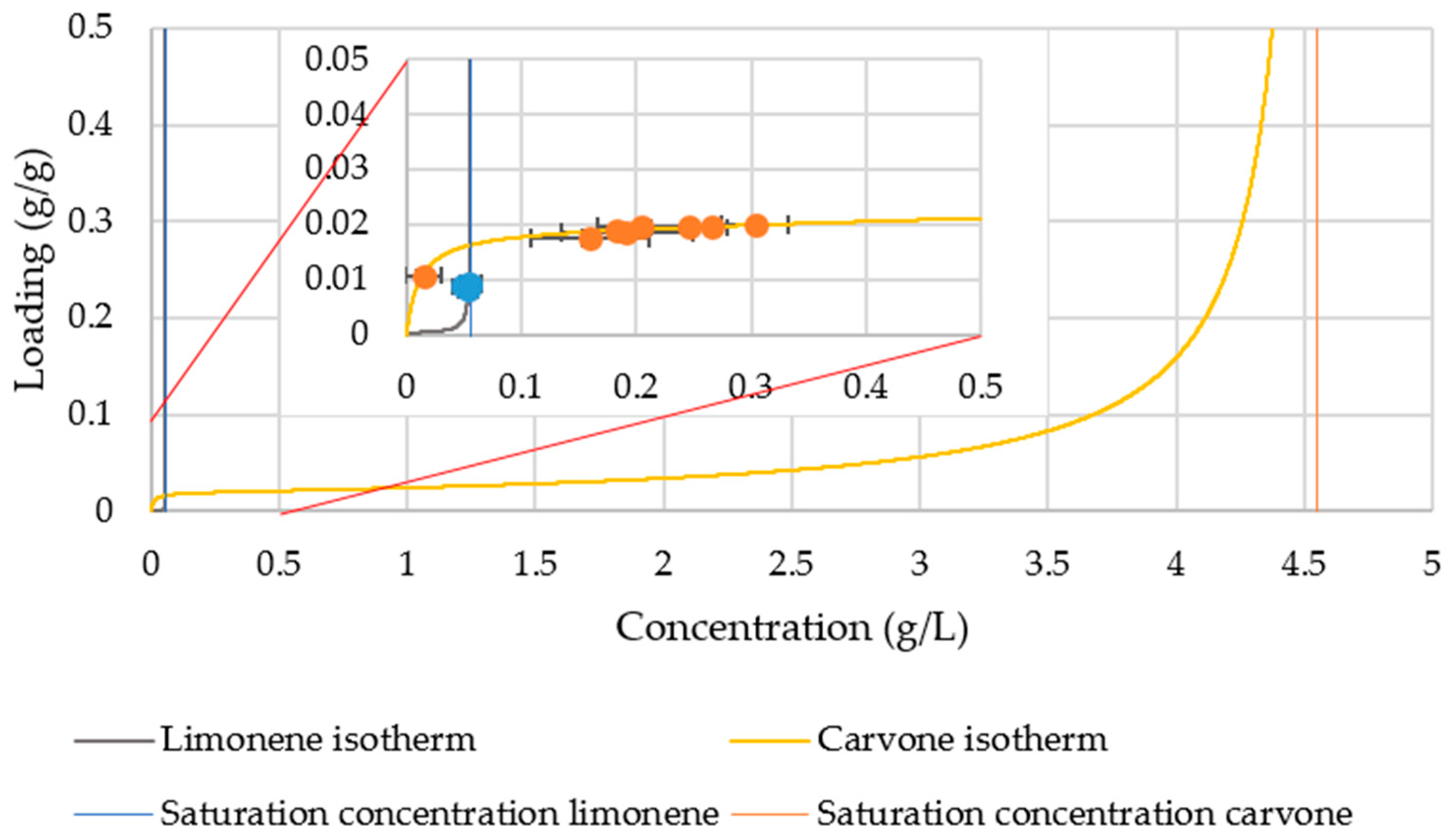
In order to determine the remaining parameters of this isotherm, the shaking tests with plant material were evaluated. For this purpose, the residual load at each measuring point was calculated using a mass balance. The experimental results and the resulting isotherm for caraway are shown in Figure 11.

For limonene, the sorption coefficient is 176 and the monolayer loading is 0.0003 g/g. For carvone, the sorption coefficient is 410 and the monolayer loading is 0.0192 g/g. For camphor, the sorption coefficient is 657 and the monolayer loading is 0.0052 g/g. For linalool, the sorption coefficient is 8400 and the monolayer loading is 0.0032 g/g.

It is noticeable that only the saturation concentration is measured for poorly soluble components. This is mainly due to the comparatively large amount of essential oil in the plant particles compared to the amount that can be dissolved in the water. In the case of more water-soluble components, such as carvone, the isotherm describes the measured experimental results. Since the wettability of the plant material is no longer guaranteed at a higher ratio to the water, less than 10% of the isotherm is covered with experimental results.

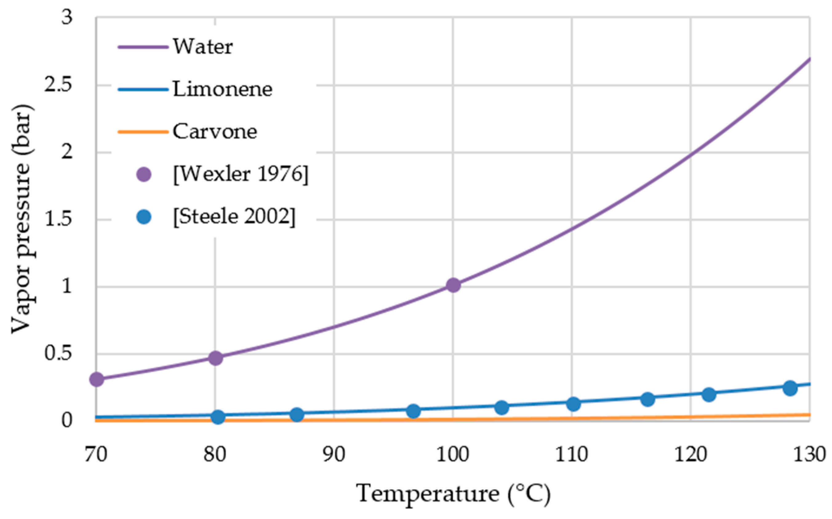
The vapour–liquid equilibrium is described using the vapour pressures of the pure substance. Therefore, the vapour pressures are transferred to the model via Aspen Properties^®. Figure 12 shows the transferred vapour pressures of limonene and carvone in comparison with literature data. It can be seen that the vapour pressures issued by Aspen Properties^® fit well with the literature values.

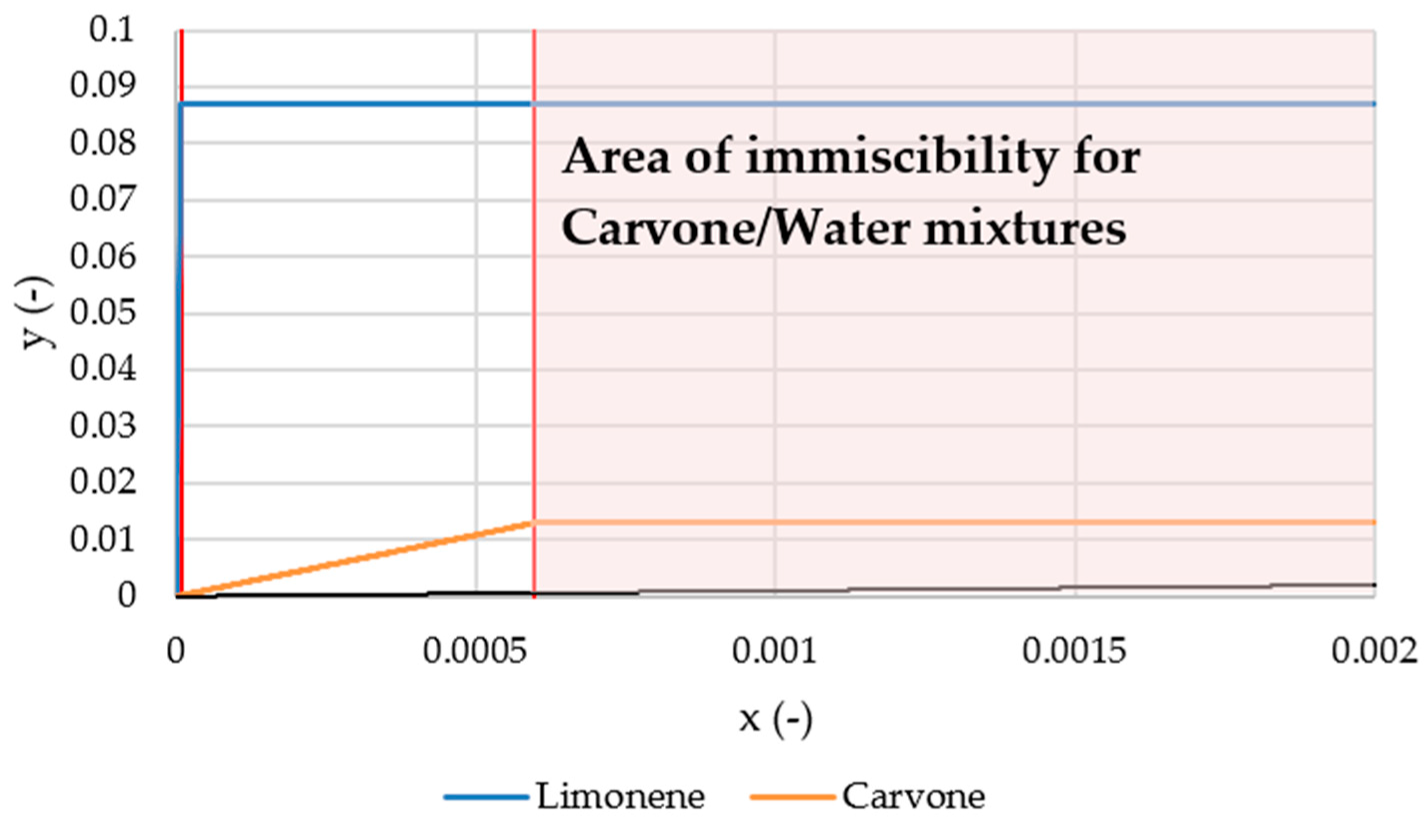
The edge area of the equilibrium diagram shown in Figure 13 is calculated using the vapour pressure of the pure components. Since the oil components are poorly water-soluble, there are two areas in the equilibrium diagram. These are separated by the solubility limit of the components. Since the solubility limit is very small, the first area considered in the diagram is also very small. In the two-phase area, the amount of substance no longer changes in the gas phase. The black line in the diagram shows the diagonal of the equilibrium diagram. The activities of the two substances are chosen so that the concentration in the vapour phase over a saturated water phase is equal to the concentration over the associated vapour phase with both phases. An activity of 125,000 is calculated for limonene and an activity of 1700 for carvone. In the literature, the activity of limonene is stated as >70,000 due to poor water solubility [48]. The calculated activity hits this area. For camphor and linalool an activity of 2400 and 2500 is calculated, respectively.

5.3.3. Mass Transfer Kinetics

For the description of the mass transport kinetics, the binary diffusion coefficient is calculated first. It is calculated using the correlation of Wilke and Chang (Equation (20)). The binary diffusion coefficient of limonene is 2.68 × ${10}^{-9}$ ${\mathrm{m}}^2$/s, that of carvone is 2.75 ×${ 10}^{-9}$ ${\mathrm{m}}^2$/s, that of camphor is 2.71 × ${10}^{-9}$ ${\mathrm{m}}^2$/s and that of linalool is 2.29 × ${10}^{-9}$ ${\mathrm{m}}^2$/s. If these values are compared with literature data, it is striking that the diffusion coefficients are around 0.5 × ${10}^{-9}$ ${\mathrm{m}}^2$/s [49]. However, these values are for 25 °C and not for 100 °C. If the Wilke and Chang correlation is evaluated at 25 °C, values of approximately 0.6 × ${10}^{-9}$ ${\mathrm{m}}^2$/s result. Hence the correlation is applied.

The pore diffusion is then calculated using the correlation of Kassing (Equation (21)). The required particle porosity is assumed to be 0.6. With the correlation there is an effective diffusion coefficient of 0.41 × ${10}^{-11}$ ${\mathrm{m}}^2$/s for limonene, 3.93 × ${10}^{-11}$ ${\mathrm{m}}^2$/s for carvone, 3.87 × ${10}^{-11}$ ${\mathrm{m}}^2$/s for camphor and 3.27 × ${10}^{-11}$ ${\mathrm{m}}^2$/s for linalool. These values are between 10–1000 times smaller than the binary diffusion coefficients and are therefore in a realistic range [27].

The mass transfer from the oil layer into the water layer is set to 1 m/s, since the oil should always be in equilibrium with the water. The height of the oil layer is assumed to be 0.0115 cm [11]. The water layer is simulated with a thickness of 1 ×${ 10}^{-5}$ cm.

The evaporation rate is calculated using Equation (19) and is 0.047 m/s during the experiment with a liquid volume flow of 3 mL/min. Values of 0.005 m/s are calculated in the literature. However, the Reynolds number in the literature is smaller by a factor of 25 [11]. The evaporation rate is therefore of the appropriate order of magnitude.

Since the cells of the caraway are broken up mechanically before the experiment, the parameters of the cell breakdown kinetics are selected so that the breakup is completed in the first seconds of the simulation. The activation energy is therefore 1 J/mol and the frequency factor is 10 1/min.

The plant hairs of lavender flowers are destroyed by water vapour. The activation energy is 1000 J/mol and the frequency factor 0.2 L/min. This leads to a cell opening rate of 0.15 L/min. In the literature, the cell opening rate for lavender flowers is 0.072 L/min [11]. The difference comes from the fact that the lavender flowers are freshly harvested in the literature, while dried flowers were used in this work. Drying leads to more unstable cell walls.

5.3.4. Model Parameter Summary

Table 5. Parameters of the accuracy and precision study of the caraway model.

Model Parameter	Unit	Limonene	Carvone	Caraway	Relative Error
Loading	(mg/${\mathrm{g}}_{\mathrm{TM}}$)	9.1	21.6	-	±3%
Maximum monolayer loading SLE	(g/L)	0.0003	0.0192	-	±3%
Equilibrium constant SLE	(-)	176.40	410.82	-	±3%
Saturation concentration SLE	(g/L)	0.056	4.55	-	±3%
Equilibrium constant LLE	(-)	0.002	0.004	-	±50%
Mass transport coefficient LLE	(cm/s)	100	100		±5%
Mean particle radius	(cm)	-	-	0.1	±3%
Bed porosity	(-)	-	-	0.4	±5%
Particle porosity	(-)	-	-	0.6	±10%
Origin	(-)			0.05	±20%
Liquid water flow rate	(mL/min)			3	±7%

summarises the determined parameters of the caraway fruits and

Table 6. Parameters of the accuracy and precision study of the lavender model.

Model Parameter	Unit	Camphor	Linalool	Lavender	Relative Error
Loading	(mg/${\mathrm{g}}_{\mathrm{TM}}$)	6.3	3.8	-	±10%
Maximum monolayer loading SLE	(g/L)	0.0052	0.0032	-	±3%
Equilibrium constant SLE	(-)	657.4	8375.82	-	±3%
Saturation concentration SLE	(g/L)	3.2	3.18	-	±3%
Equilibrium constant LLE	(-)	0.005	0.002	-	±100%
Mass transport coefficient LLE	(cm/s)	100	100		±5%
Mean particle radius	(cm)	-	-	0.15	±3%
Bed porosity	(-)	-	-	0.4	±5%
Particle porosity	(-)	-	-	0.6	±10%
Origin	(-)			0.15	±5%
Liquid water flow rate	(mL/min)			3	±7%

summarises the determined parameters of the lavender flowers.

5.4. Model Validation

For the validation of the developed model, the precision and accuracy of the model results are first checked at the central point of the test plan. The precision of the model results from the error range of the model parameter determination shown in Table 5 and Table 6. The relative errors originate from the experimental errors of the model parameter determination and result, for example, from measurement inaccuracies [12].

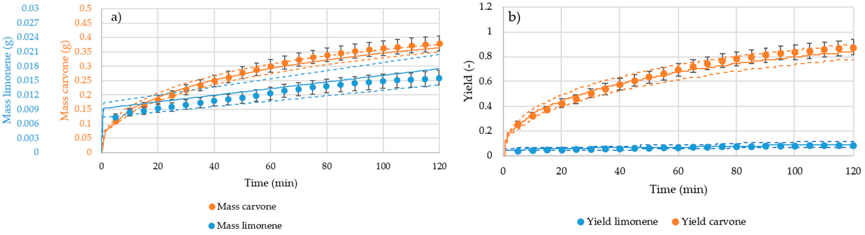
Simulations are carried out with the determined model parameters and with the maximum possible error of the model parameters, to show whether the simulation has a higher accuracy and precision than the affiliated experiment. This leads to the accuracy, which is shown with a solid line. The fluctuation range of the simulation is shown as a dashed line. The accuracy and precision are displayed in Figure 14 for the mass and yield of the caraway system.

In the experiments at the central point, a mass of 378 ± 16 mg carvone and a mass of 16 ± 1 mg limonene are obtained. This corresponds to a yield of 87 ± 6% carvone and a yield of 9 ± 1% limonene. The simulation calculates a mass of 364 mg for the carvone and a mass of 17 mg for the limonene. This corresponds to a yield of 84% of the carvone and a yield of 9% of the limonene. The precision of the simulation is ±13 mg for the mass of carvone, ±3 mg for the mass of limonene, ±6% for the carvone yield and ±2% for the limonene yield. The simulation results of the carvone have a higher precision than the results of the experiments carried out at the central point of the test plan. The simulation results of limonene are less precise than the experiments. The prediction inaccuracy doubles and increases from 7% to 16%. This is mainly due to the low extracted mass and the low water solubility of limonene. These effects have already caused problems when determining model parameters. Despite less precision, the model gives a good prediction of the simulation results in the case of the caraway.

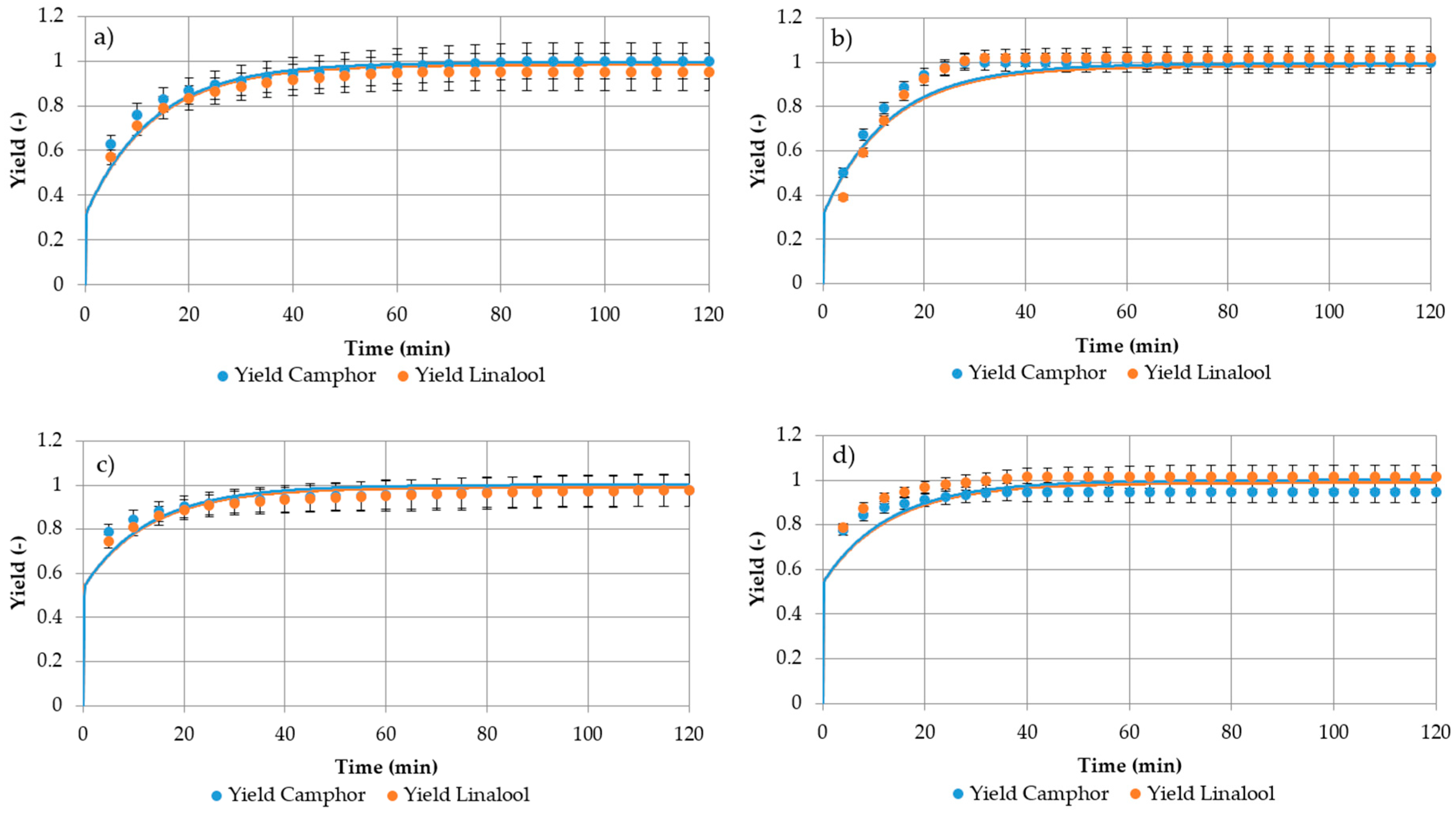
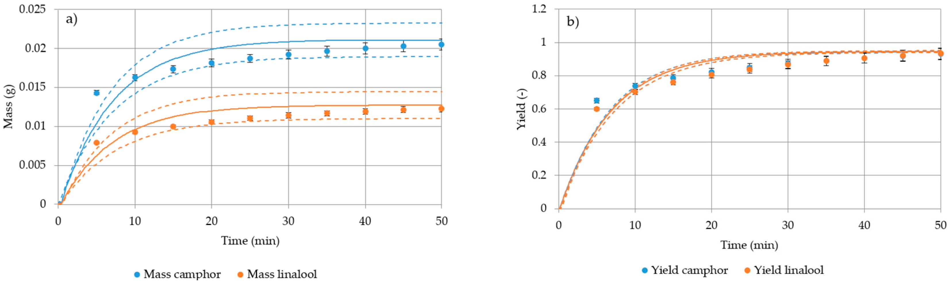
For the mass and the yield of the lavender system, the accuracy and precision are displayed in Figure 15.

Since the extraction is complete after 50 min, the values at 40 min are used to discuss accuracy and precision. In the experiments a mass of 21 ± 1 mg camphor and a mass of 13 ± 1 mg linalool are obtained. This corresponds to a yield of 96 ± 4% camphor and a yield of 96 ± 4% linalool. The simulation calculates a mass of 21 mg for camphor and a mass of 13 mg for linalool. This corresponds to a yield of 94% camphor and a yield of 9% linalool. These values show that the simulation is highly accurate at the central point of the experimental design. The fluctuation of the simulation results from the model parameter determination is 2 mg for the mass of camphor, 2 mg for the mass of linalool, 1% for the yield of camphor and 1% for the yield of linalool. The simulation results of the yield have a higher precision than the experiments. The simulation results of the extracted mass are less precise than the experiments. The inaccuracy increases from 1 mg to 2 mg. This is mainly due to the low mass to be extracted and the great uncertainty regarding the maximum loading of the plant particles. If the maximum load is determined with a higher precision, the precision of the simulation results will also improve. However, the figures also state that the simulation should underestimate the extraction speed at the beginning and overestimate it at the end. This is probably due to poorly chosen initial conditions, since the essential oil is evenly distributed in the bed at the beginning of the simulation. In addition, the bed at the beginning of the simulation is at the boiling point of the water. This means that an essential oil is discharged from the filling right at the beginning of the simulation. In reality, the essential oil is evaporated during the heating phase at the lower end of the bed and then condenses in the part of the bed which is still to be heated. This leads to a distribution gradient in the bed. This effect is more pronounced in the lavender system because the essential oil is easier to evaporate due to the location in the plant hairs [32]. Since this effect is greater with a higher sample of plant material, it is advisable to simulate the heating phase and the temperature front running through the bed.

All in all, the model precision and accuracy are comparable with the affiliated experiments at the central point of the experimental design.

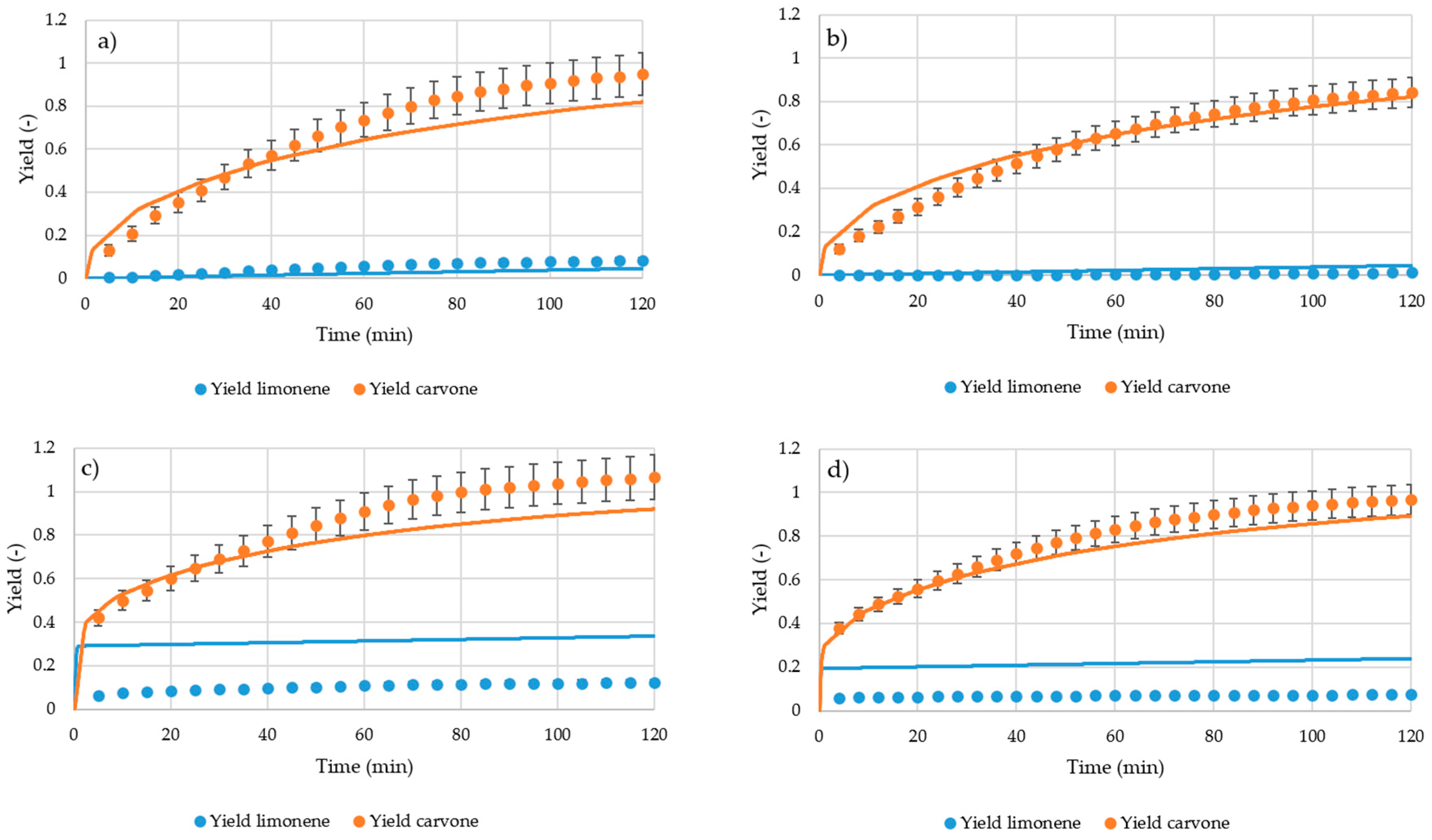
For further validation of the model, an accuracy check is carried out at the corner points of the design space. This is done first for the caraway system. The simulation results are shown in Figure 16.

The focus of the analysis is on carvone, due to low yield and consequently poor measurability of limonene. It can be seen that the simulation reproduces the experimental results well. The model for the caraway system is therefore comparable to the affiliated experiments.

For the lavender system it has already been shown that the initial distribution has to be adjusted. The starting conditions for extraction assume that the target components are evenly distributed at the start of the extraction, which is shown in the left side of Figure 17. This assumption is not valid for oil, which is easily vaporised from the plant material between start of the extraction and the collection of the first condensate.

This can be seen more clearly at the corner of the statistical test plan, at which 5.4 g lavender were weighed (Figure 17). To increase the accuracy of the simulation, the impact of the initial heating phase and the initial target component distribution has to be considered. This adjustment is shown in Figure 17. With this adjustment, the corner points of the lavender system are simulated. The results and comparison to the experimental results are shown in Figure 18.

It can also be seen in this case that the simulation results agree well with the experimental results. Overall, the model is comparable to the experimental results.

5.5. Scale-Up and Industrial Application

This chapter checks whether the simulation also delivers results on an industrial scale. It also shows how the simulation can improve the yield and profit of the steam distillation.

A distillation bubble with a diameter of 1.4 m and a height of 2.65 m is used as an industrial scale. This corresponds to a volume of 4.08 ${\mathrm{m}}^3$. The filling level of the bed is 4/5 of the bubble height. The bed is flowed through with 300 kg of water vapour per hour for 2.5 h. The first product drops are obtained after 30 min. Distillation is continued for 2 h after receiving the first drops. The simulations start when the first drop of product leaves the still. In Figure 19, the difference between industrial and laboratory scale of the caraway system is shown.

In the first simulation in the industrial scale, 10% of the essential oil was initially set free through mechanical actions. In this case, 26.7 kg of the 46.5 kg essential oil are obtained after 120 min. This corresponds to an overall yield of 57%. The plant material is not completely exhausted after two hours. To optimise the process, a higher degree of disruption can be generated through more mechanical stress. Figure 20 displays the simulated yield of the caraway system, when 30% of the essential oil are set free. The figure shows that the plant material is still not completely exhausted after two hours. Now 33.5 kg are extracted, which corresponds to an increase of 6.8 kg. The yield increases by 15% to 72%. In addition to that, Figure 20 shows how long it makes sense to continue the optimised steam distillation. In this calculation, costs of 60 € per ton of water vapour are assumed [50]. In addition, an employee is required to operate steam distillation. This employee is estimated with 100,000 € per year. The essential oil of caraway is available for 0.695 € per mL [51]. Of this price, 20% will be used for taxes, 40% for marketing and sales, 15% for the required plant material and 5% for maintenance and investments. The remaining 20% are divided between the operating costs and the return on steam distillation. It can be seen that the operation of the plant is still profitable after 120 min. However, losses of oil in the distillation water that lead to a reduction in the yield are considered in the calculation, as they depend on the process conditions during condensation. Accordingly, it still has to be checked whether extracted oil can be separated after 120 min.

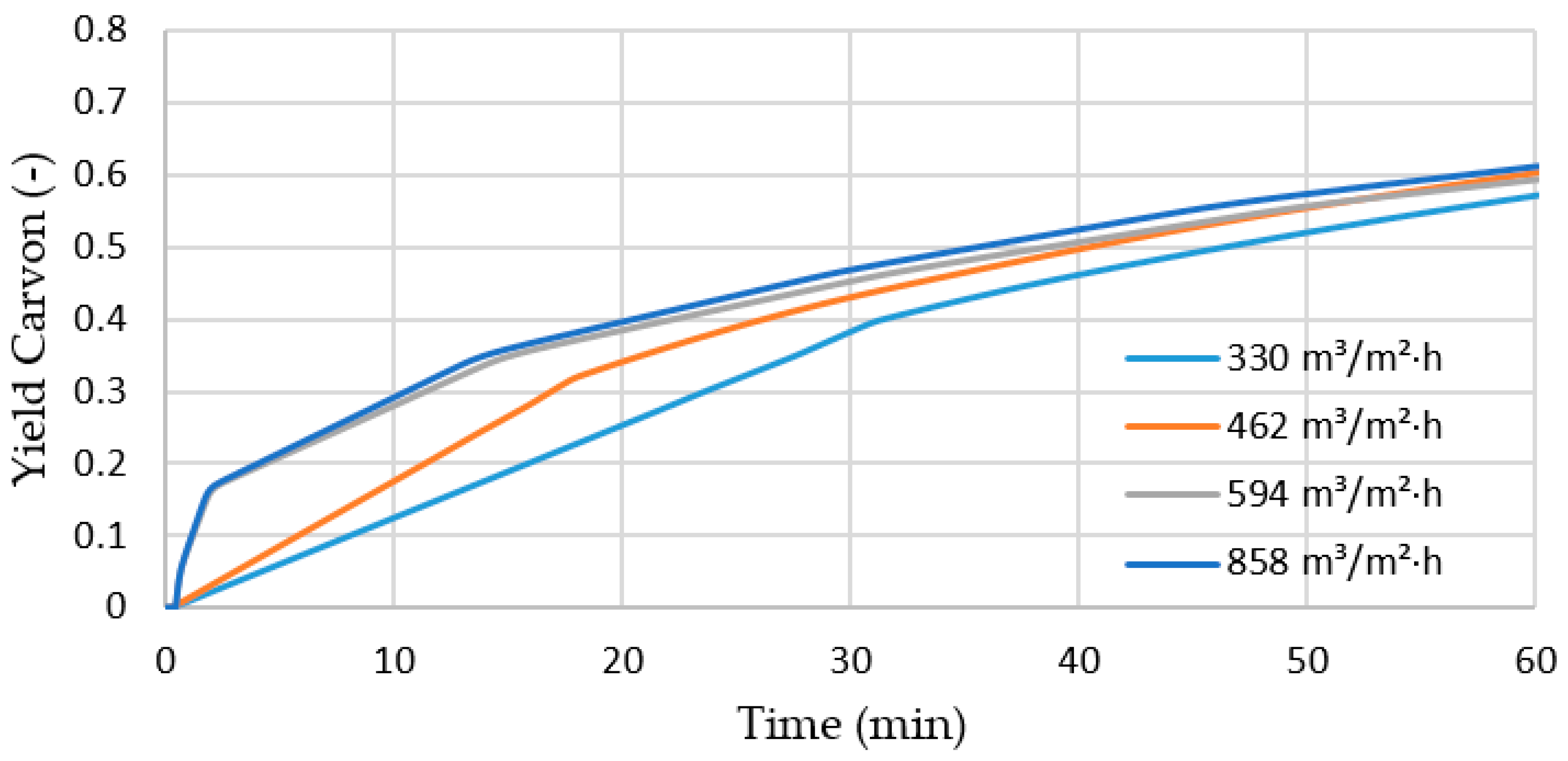
The process model can be used to optimise the distillation process, for example, by evaluating the effect of higher steam flowrate on the extraction. This optimization is shown in Figure 21 and shows that an increase in flowrate, to circumvent a possible equilibrium limitation, decreases the time needed for vaporization of the free oil.

The increase in flowrate impacts the initial vaporization of oil as expected and increases the yield in the first 10 min. The investment in higher flowrate does not yield significant improvement after the first 10 min, as the diffusion limitation dominates in this state of the extraction.

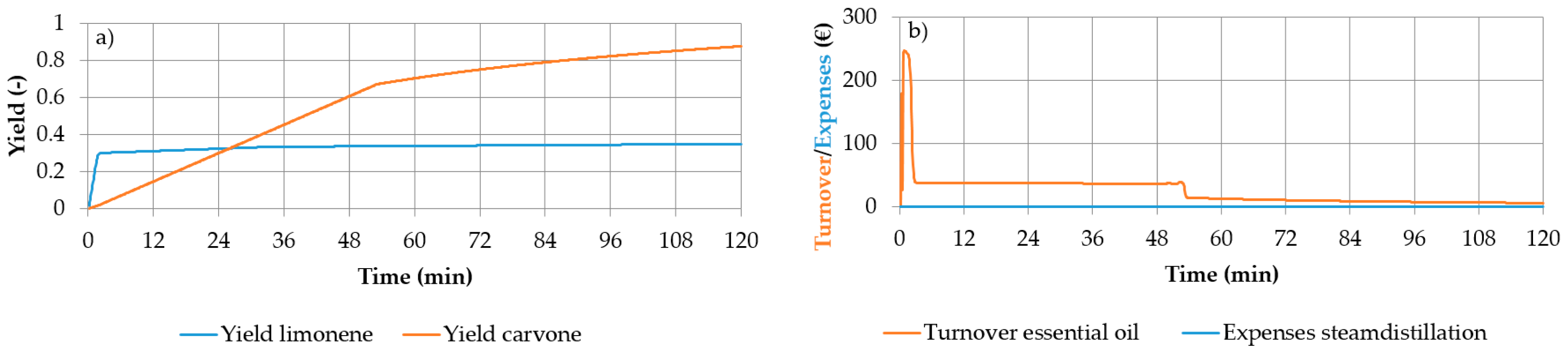
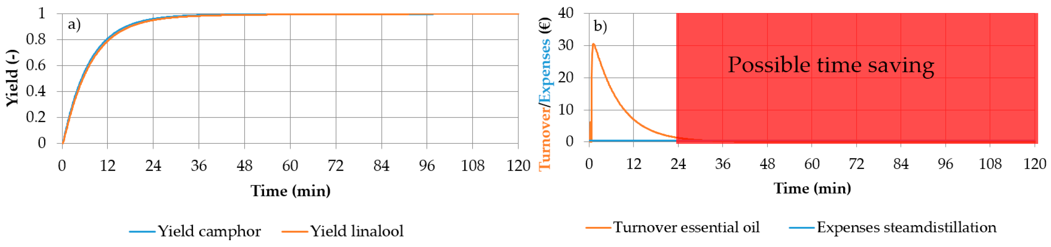
Figure 22 displays that all of the essential oil is extracted during steam distillation of lavender. It can also be seen that the two substances are not limited by the vapour phase. This can be seen from the fact that the derivation of the function is continuous. To optimise steam distillation, how long the distillation should continue is checked. For this, the same assumptions are made as when considering the caraway system. Only the price for lavender oil is adjusted to 0.595 € per mL of lavender oil [52]. The figure shows that steam distillation is completed after 40 min. A total of 3.2 kg of essential oil is obtained during the distillation. However, the costs exceed the profit after only 32 min. As a result, the extraction can be stopped after this time. This corresponds to a savings of 440 kg of steam and 95 € in personnel costs per batch. In addition, more than twice the number of steam distillation processes are possible at the same time. This leads to an increased throughput of plant material, doubling turn-over at constant fixed costs.

As summarised in

Table 7. Summary of model-based optimizations for steam distillation.

Plant System	Actual State	Optimization Parameters	Optimised State
Caraway	57% yield	Degree of disintegration pre-treatment and specific energy amount 50%	72% yield
	120 min		120 min
	14,800 € turnover/batch		18,600 € turnover/batch
	2 distillations/day		2 distillations/day
Lavender	100% yield	Extraction time and vapour amount 1/4	100% yield
	120 min		32 min
	2400 € turnover/batch		2400 € turnover/batch
	2 distillations/day		3 distillations/day

, profit is maximised in diffusion-inhibited plant systems, such as the caraway system, by increasing the degree of disintegration by pre-treatment. This increases the turnover, which is achieved per batch in 120 min. In the case of plant systems with superficial oil, such as the lavender system, total extraction does not take 120 min but about 1/4th the time. Thus, the profit maximization with superficial oil is achieved by increasing the throughput factor 4 and reducing vapour (i.e., energy amount per batch by a factor of 4).

The simulation results on the industrial scale demonstrate that the simulations provide a better understanding of the extraction system. With the help of the model yield, energy amount, plant and equipment resource utilization and finally profit can be maximised.

6. Discussion and Conclusions

A predictive general physico-chemical process model for steam distillation was developed in order to generate a digital twin for process optimization and process integration up to advanced process control and life-cycle analysis. To gain a verified and validated model, the process model development workflow (Figure 3) presented by Sixt et al. [12] is applied.

The first segment in this workflow is the model derivation and implementation. Therefore, a literature search was carried out to elaborate current model approaches. It has been found that, when modelling steam distillation, a distinction must be made between the extraction of essential oil from superficial plant hairs and from the interior of the plant particle. Furthermore, a plausibility study was carried out to verify the derived and implemented model. It was shown that the variables have a plausible physical behaviour and that all mass balances are closed. Due to this, the derived model is verified. The correct implementation of all model equations can be reviewed, avoiding additional efforts for quality assurance during later stages of model validation. This verification of the model structure is an important basis for further model development and the first major milestone in model development.

In the second segment, a sensitivity study was carried out to identify significant parameters. The identification of significant parameters based on experimental data is important to confirm that all required mass transfer effects are recognised in the model. It turned out that the breakup rate, the origin, the saturation concentration in the liquid phase, the effective diffusion coefficient and the mean particle radius are significant for the obtained yield. This observation is in line with the set expectations. It should be considered that the inclusion of seemingly insignificant parameters is important to maintain a comprehensive model approach. One example is the liquid–liquid equilibria, which are insignificant for both model systems characterised in this study. Nevertheless, the exclusion of this effect limits the usability for systems with higher distribution of target components into the water phase.

For the third segment the accuracy and precision at the central point of the statistical design was evaluated. It turned out that the model is highly accurate at the central point. Further improvements to the model accuracy are certainly possible, as shown by the increase of model accuracy for early phases of the extraction of oil in the lavender system. By adapting the initial conditions when considering superficial essential oil, the results at the central point of the test plan are comparable with affiliated experiments.

The precision of the model is in the area of the carried-out steam distillation experiments. This is a requirement for a physico-chemical model, to generate results comparable to experimental data and substitute laboratory work with simulations. Poorly soluble components, such as limonene, are less precise than more soluble components.

In the fourth segment, the accuracy at the corner point of the statistical plan was checked. With the adjustment of the initial conditions, the results are again comparable with the associated experiments. The benefit of such a validated predictive model is shown in the case study. Since the model separates the mass transfer effects, and model parameter and fluid dynamics are implemented separately, the model can be applied to simulate industrial-sized scale-up distillations. It was found that the yield and throughput of industrial steam distillations can be improved with this model. The optimization strategy depends on extraction characteristics. The increase in yield by a higher steam flow is offset by diffusion limitations. This highlights the benefit of the developed model, as individual optimization strategies can be developed for different target components in one model.

Overall, a verified and validated model for steam distillation was developed as shown in this article. The model includes all possible extraction mechanisms and phenomena and thus contributes to a better process comprehension needed for optimization of steam distillation and can be applied to different plants and target components. Since focus of the model is on the technical application and because the simulation results also have a sufficiently high precision, the model provides a good basis for further process optimization and process integration in order to support process development and plant optimization up to advanced process control with the aid of a model-based digital twin (i.e., now available).