CFD and Experimental Characterization of a Bioreactor: Analysis via Power Curve, Flow Patterns and
k
L
a

 ,
,  and
and
Abstract
:
1. Introduction
2. Literature Review
2.1. Previous Work
2.2. Dimensionless Numbers
2.3. Oxygen Diffusion
Minimum to Cell Culture
2.4. Governing Equation
2.4.1. Continuity Equation
2.4.2. Momentum Equation
2.4.3. Turbulence Model
2.4.4. Eulerian Multiphase
3. Materials and Methods
3.1. Experimental Methods
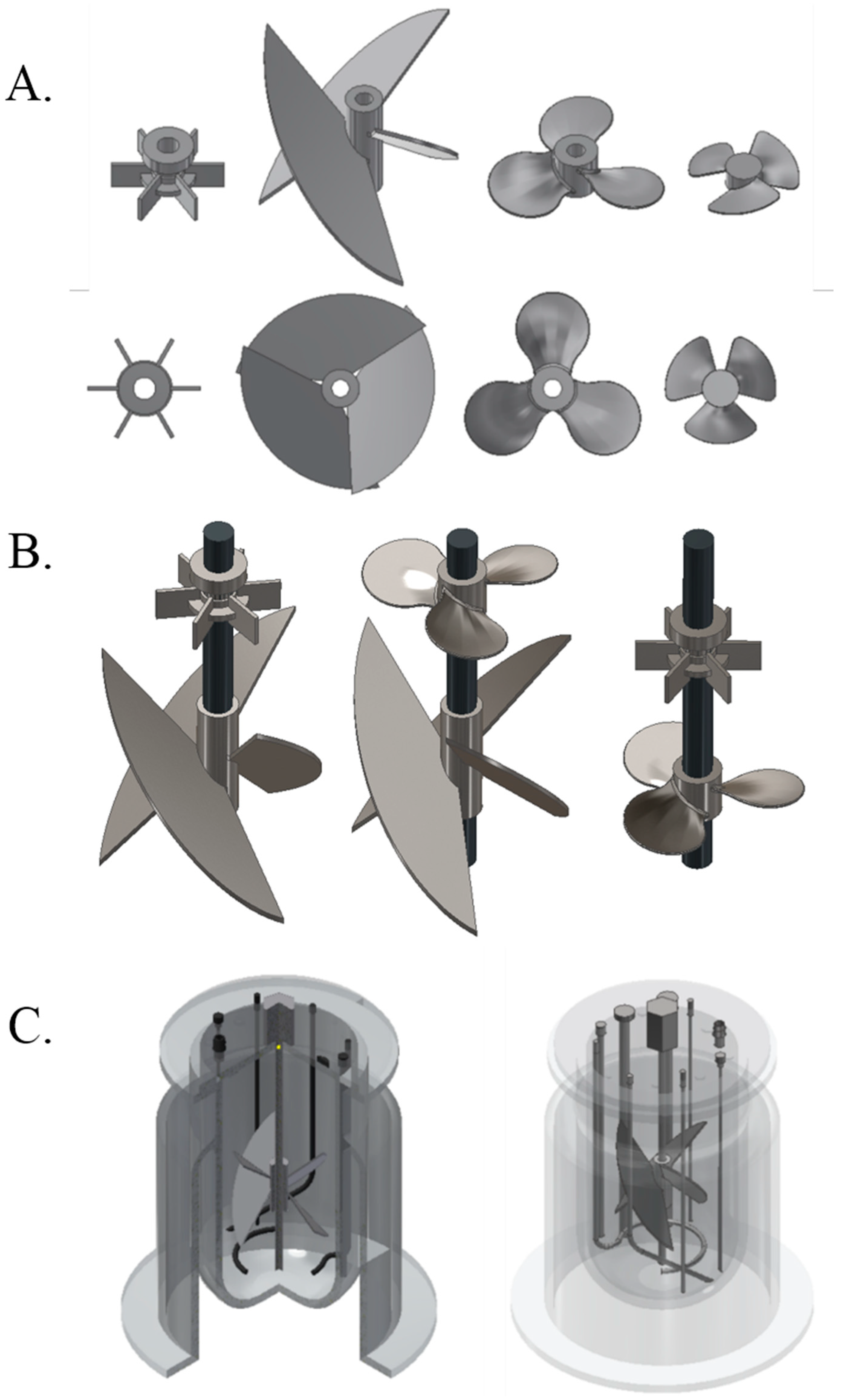
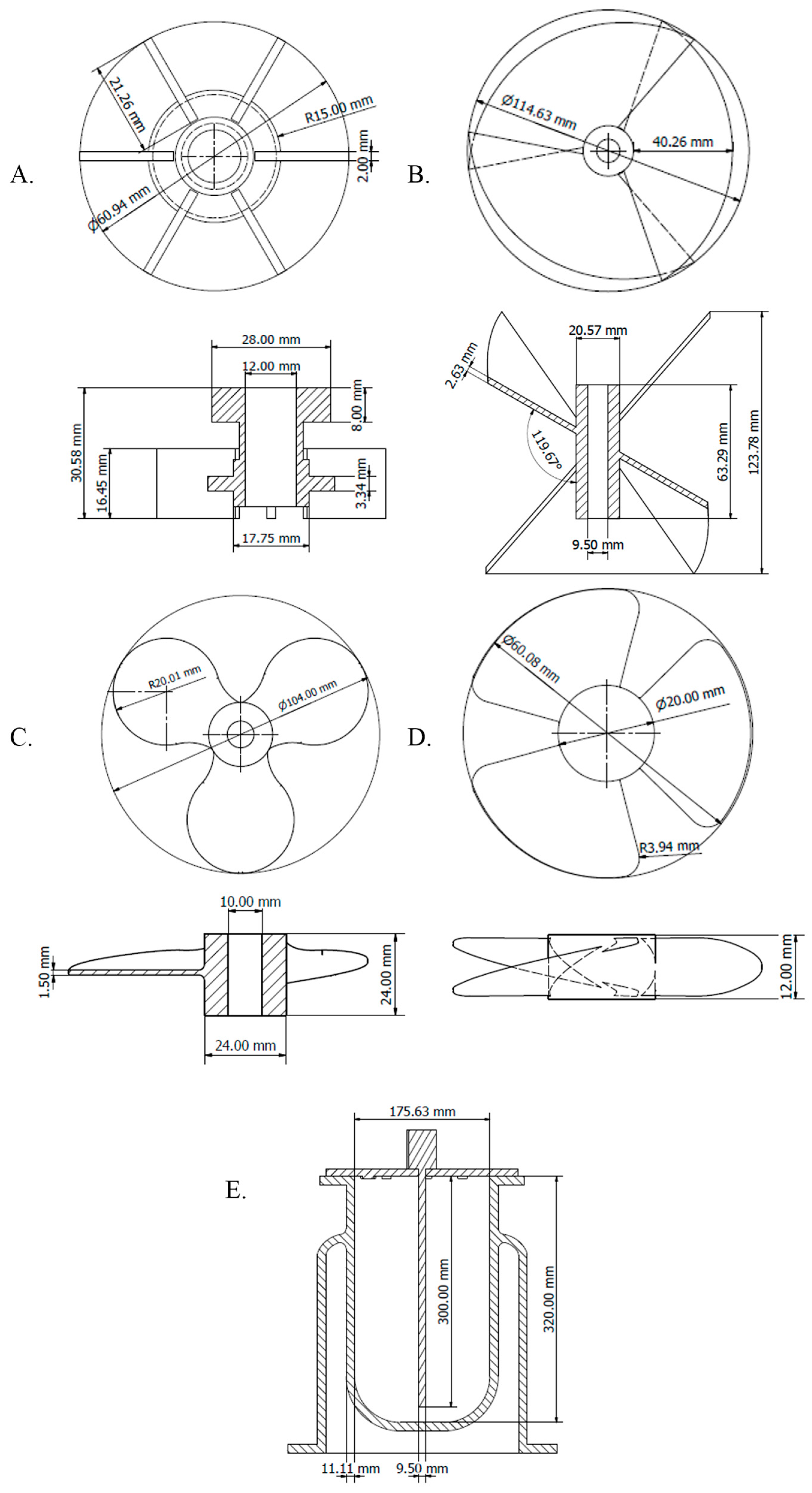
3.1.1. Impeller Design
3.1.2. Power Curve Determination
3.1.3. Determination by Gassing Out Method
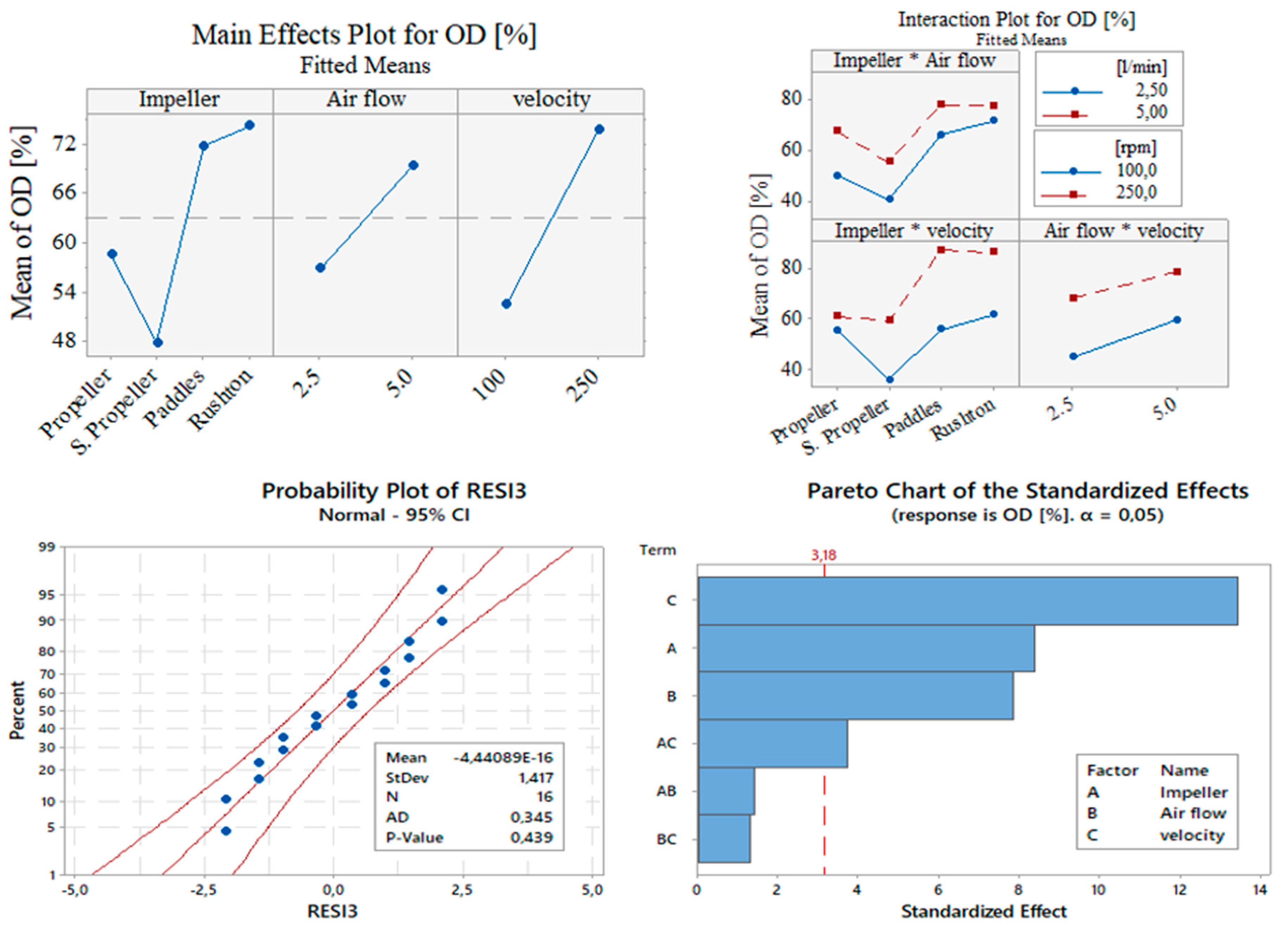
3.1.4. Experimental Design to Establish Operational Effects in Dissolved Oxygen
3.1.5. Flow Patterns
3.2. CAD and Mesh Construction
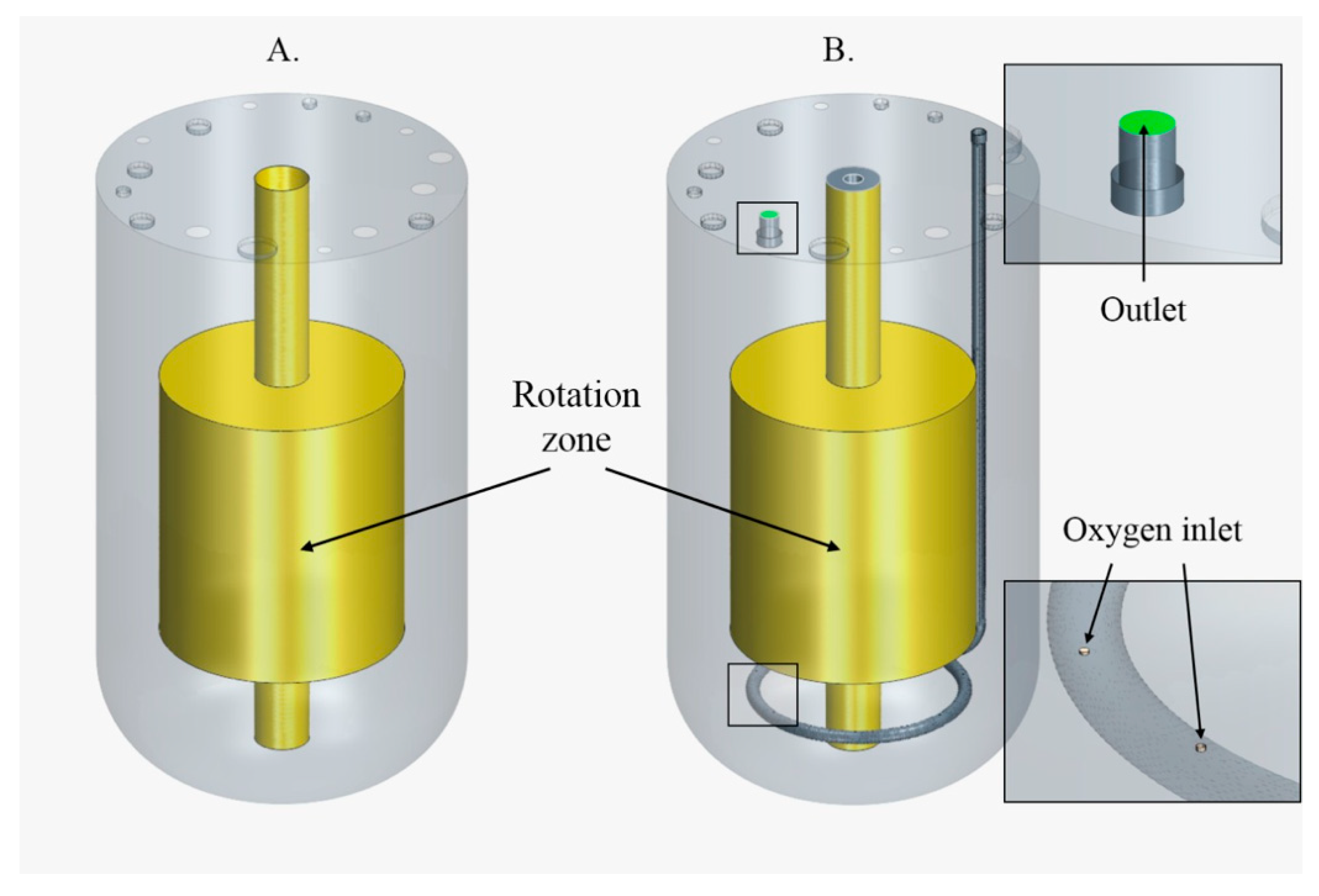
3.2.1. Bioreactor Dimension and Geometry Design in Autodesk Inventor Software
3.2.2. Mesh Independence and Preliminary Configuration
Qualitative Method
Quantitative Method–GCI Calculation
3.3. Modeling Approach
3.3.1. Power Analysis
3.3.2. Flow Patterns Analysis
4. Results and Discussion
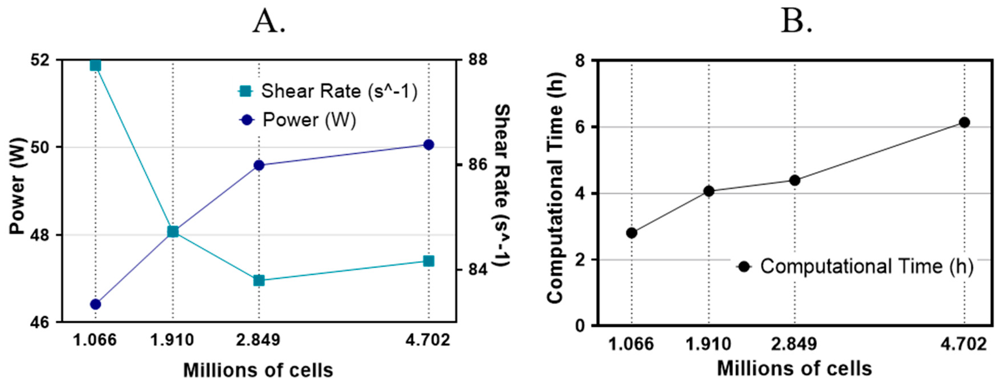
4.1. Mesh Independence
Mesh Independence Analysis
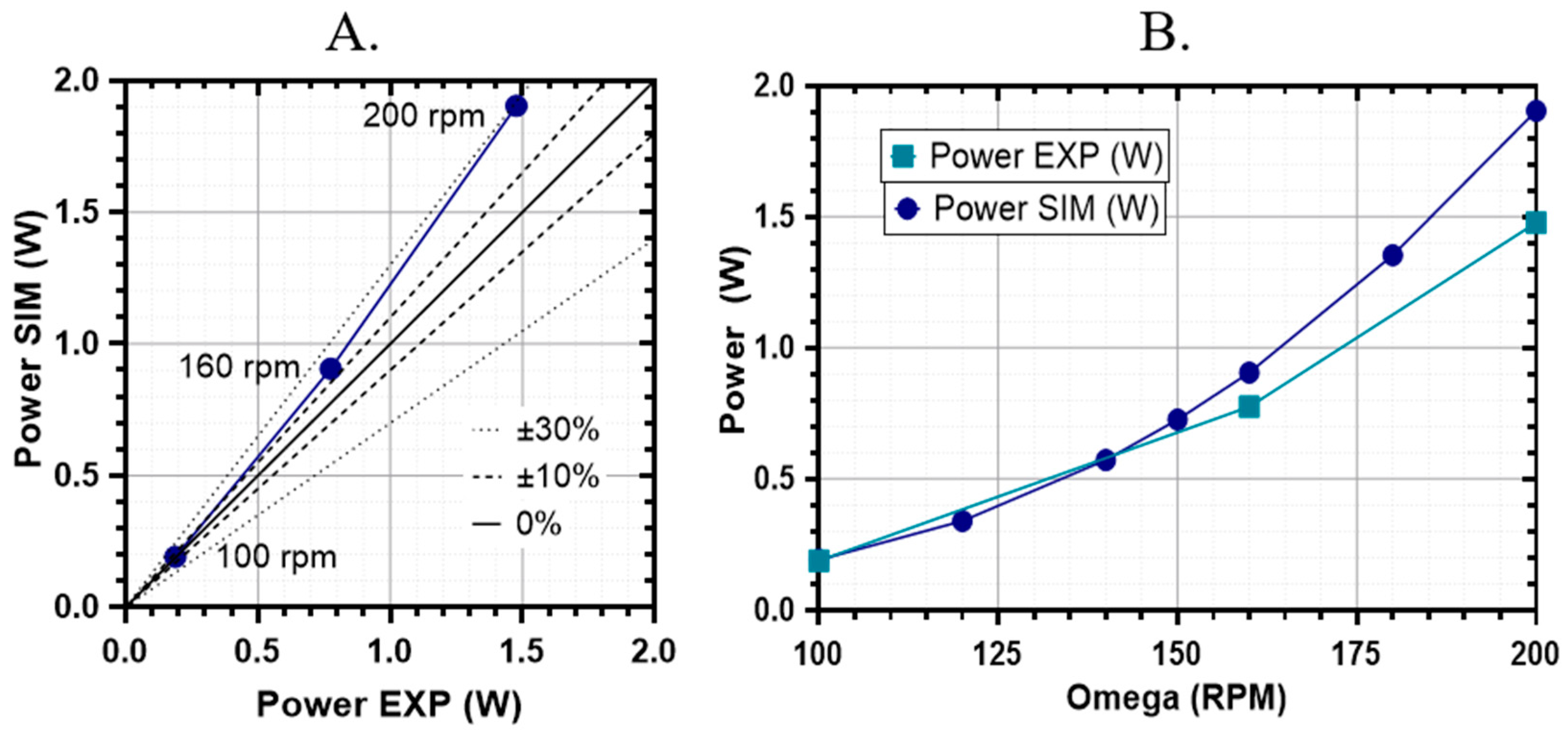
4.2. Simulation Model Validation
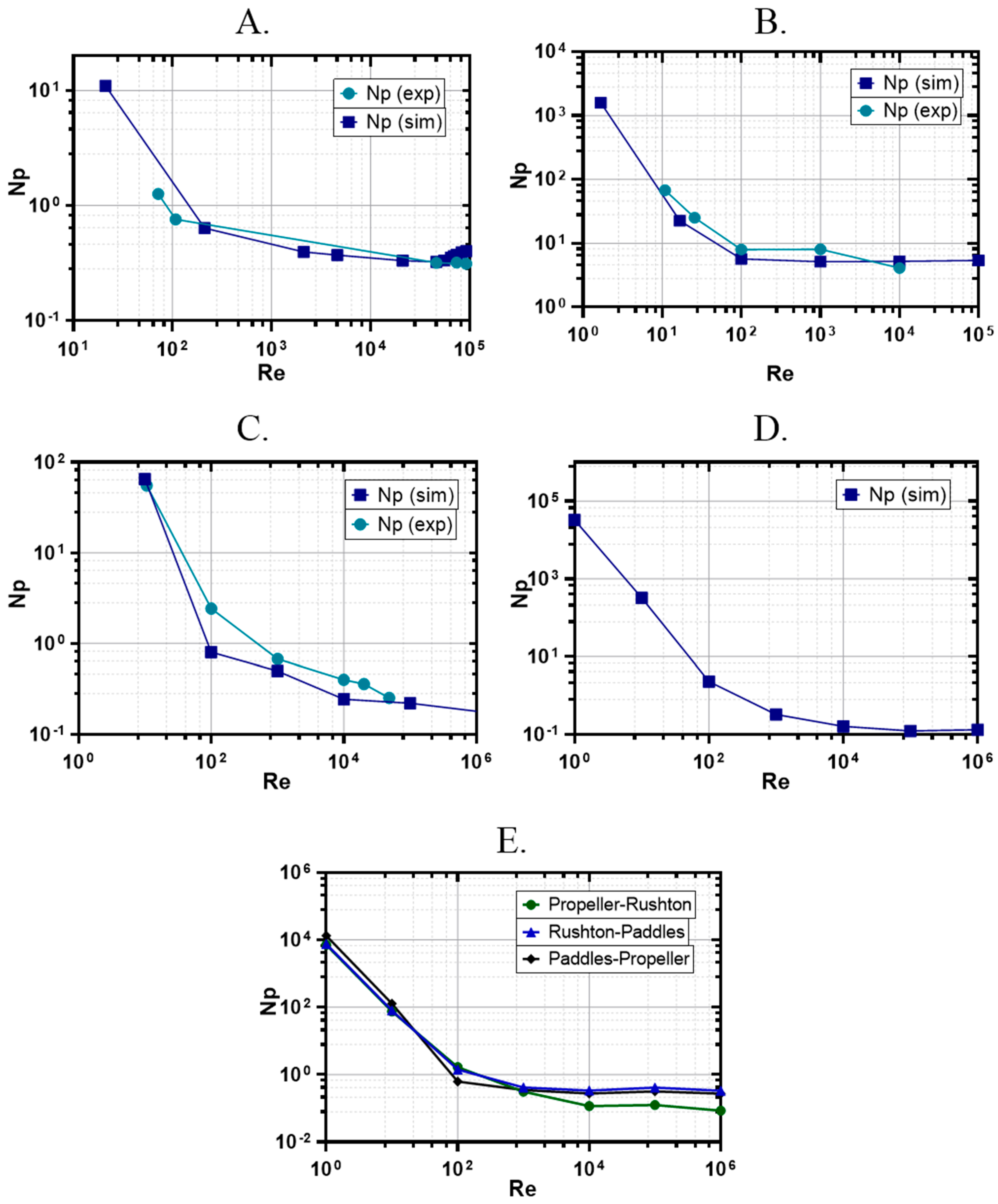
4.3. Power Analysis
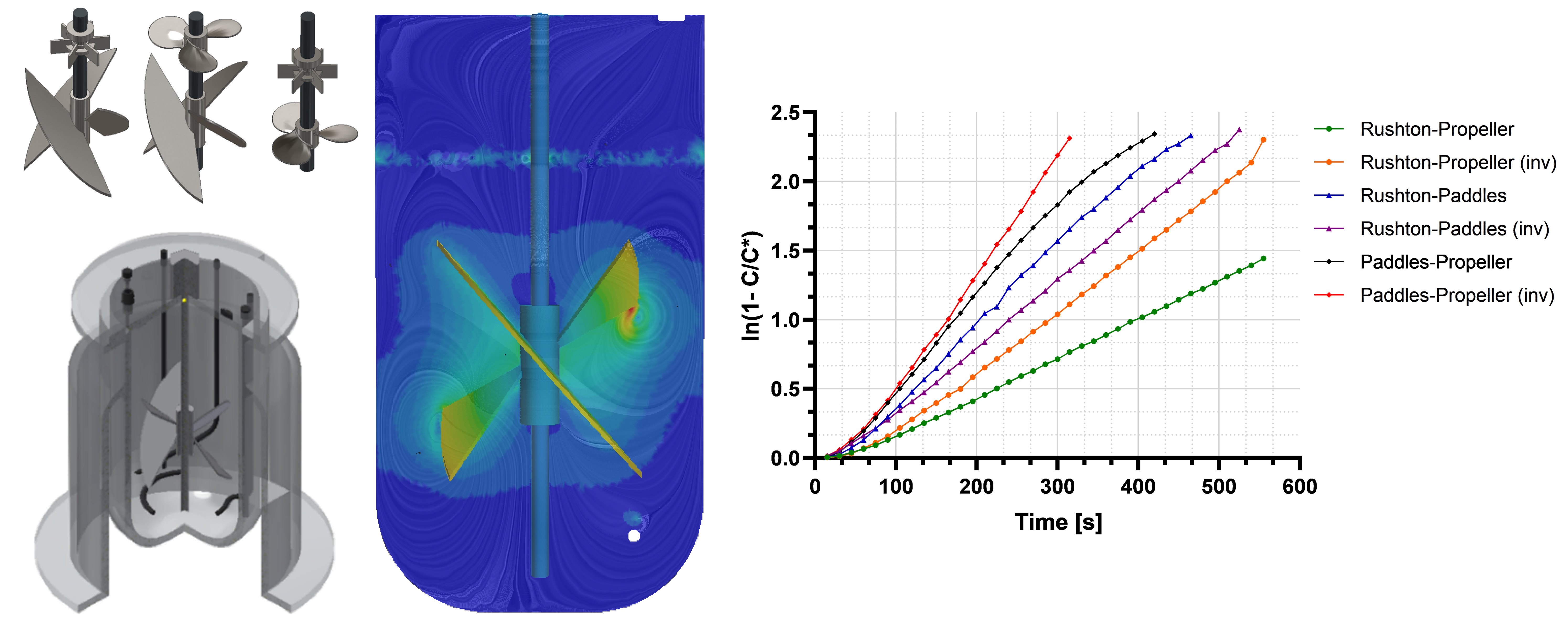
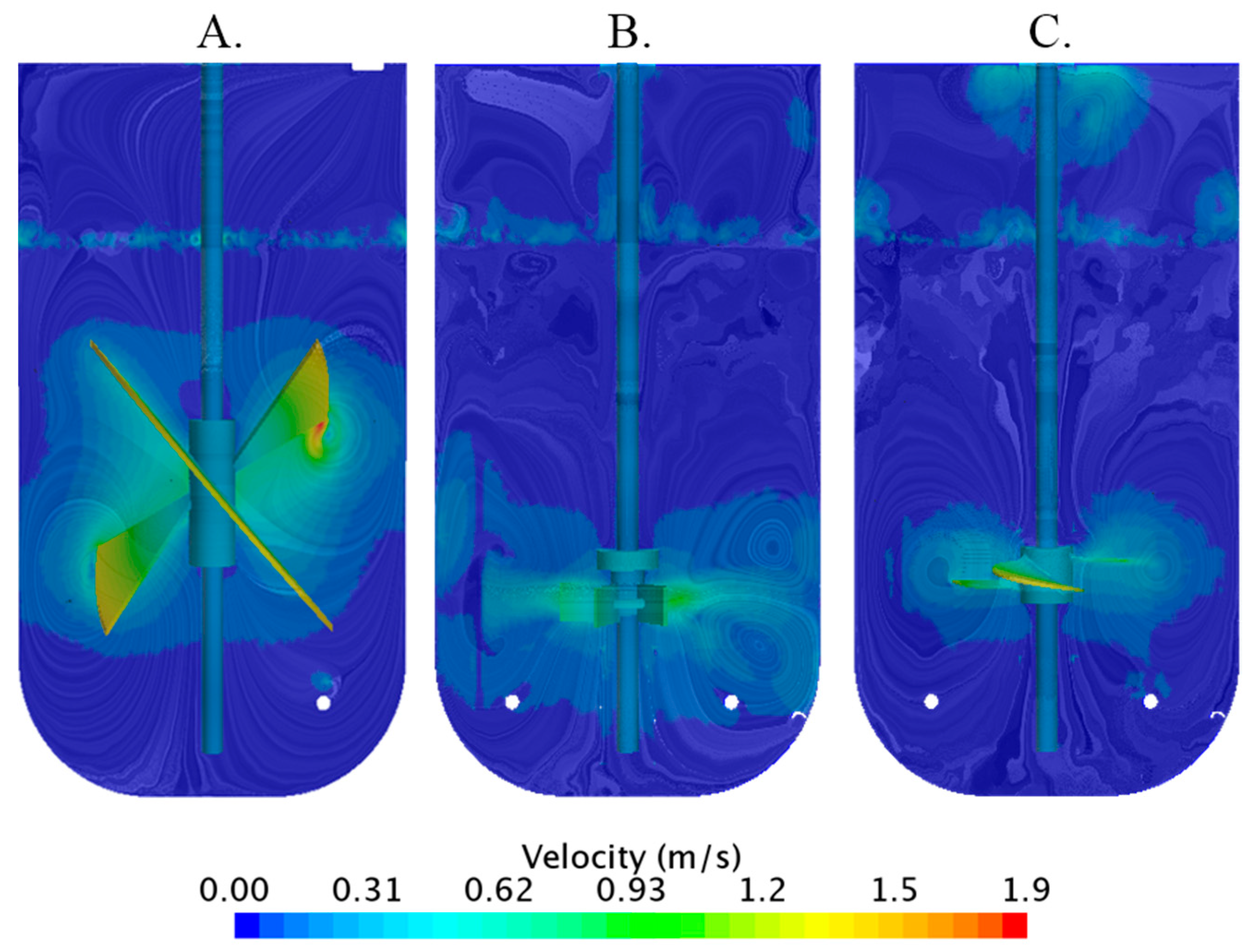
4.4. Flow Patterns
4.5. Oxygen Diffusion
4.5.1. Experimental Design
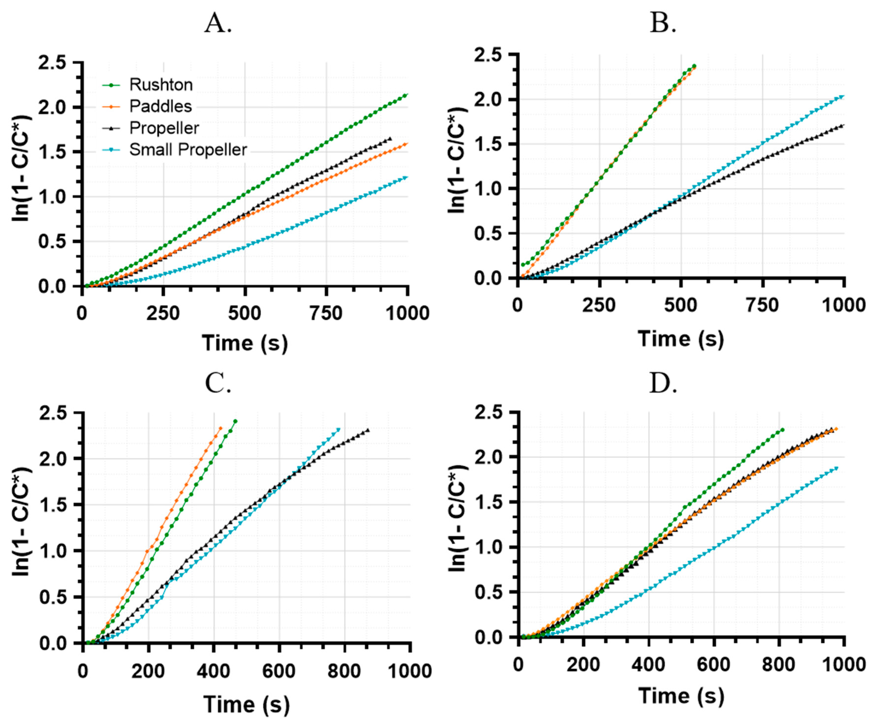
4.5.2. Determination
One Impeller
Impeller Combinations
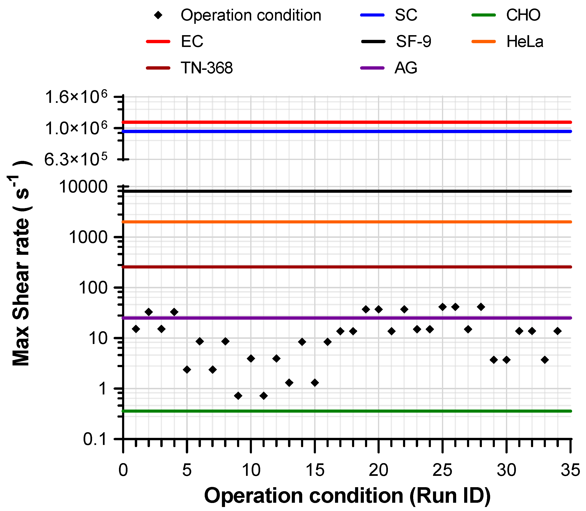
Shear Rate
5. Conclusions
Author Contributions
Funding
Acknowledgments
Conflicts of Interest
Nomenclature
Romanic symbols
| Gas–liquid interfacial area | ||
| Oxygen concentration in the gaseous phase | ||
| Oxygen concentration in the liquid phase | ||
| Oxygen concentration in equilibrium with gaseous phase (oxygen solubility) | ||
| Critical oxygen concentration to ensure the cell culture growth | ||
| Diameter | ||
| GCI relative error-index | ||
| DF | Degrees of freedom | |
| Binary diffusion coefficient | ||
| Molecular diffusivity | ||
| Grid Convergence Index | ||
| Molar flux of component | ||
| Mass transfer coefficient in the gaseous phase | ||
| Mass transfer coefficient of | ||
| Mass transfer coefficient in the liquid phase | ||
| MS | Mean square | |
| Angular velocity | ||
| Molar transfer rate of A | ||
| Power number | ||
| Pumping number | ||
| Power | ||
| Specific uptake rate | ||
| Total flow | ||
| Volumetric oxygen uptake rate | ||
| Reynolds number | ||
| Reynolds-Average Navier–Stokes | ||
| SS | Sum of square | |
| Time | ||
| Temperature | ||
| Velocity vector | ||
| Volume of Fraction | ||
| Cell concentration in the broth | ||
| Water fraction in solution | ||
| Cartesian plane coordinate |
Greek symbols
| Viscosity | ||
| Density | ||
| GCI analysis variable |
Appendix A. Data S1. GCI Step by Step Calculation


| StdOrder | RunOrder | PtType | Blocks | Impeller | Airflow | Velocity | DO (%) |
|---|---|---|---|---|---|---|---|
| 12 | 1 | 1 | 1 | Paddles | 5.0 | 250 | 90.3 |
| 2 | 2 | 1 | 1 | Propeller | 2.5 | 250 | 52.2 |
| 3 | 3 | 1 | 1 | Propeller | 5.0 | 100 | 64.0 |
| 6 | 4 | 1 | 1 | Small Propeller | 2.5 | 250 | 52.2 |
| 13 | 5 | 1 | 1 | Rushton | 2.5 | 100 | 57.4 |
| 7 | 6 | 1 | 1 | Small Propeller | 5.0 | 100 | 43.5 |
| 9 | 7 | 1 | 1 | Paddles | 2.5 | 100 | 46.9 |
| 11 | 8 | 1 | 1 | Paddles | 5.0 | 100 | 64.9 |
| 5 | 9 | 1 | 1 | Small Propeller | 2.5 | 100 | 28.8 |
| 1 | 10 | 1 | 1 | Propeller | 2.5 | 100 | 47.6 |
| 16 | 11 | 1 | 1 | Rushton | 5.0 | 250 | 88.2 |
| 14 | 12 | 1 | 1 | Rushton | 2.5 | 250 | 84.9 |
| 15 | 13 | 1 | 1 | Rushton | 5.0 | 100 | 66.2 |
| 4 | 14 | 1 | 1 | Propeller | 5.0 | 250 | 70.3 |
| 10 | 15 | 1 | 1 | Paddles | 2.5 | 250 | 84.7 |
| 8 | 16 | 1 | 1 | Small Propeller | 5.0 | 250 | 66.8 |
| Source | DF | Adj SS | Adj MS | F-Value | p-Value |
|---|---|---|---|---|---|
| Model | 12 | 4694.14 | 391.18 | 38.96 | 0.006 |
| Linear | 5 | 4234.85 | 846.97 | 84.35 | 0.002 |
| Impeller | 3 | 1803.46 | 601.15 | 59.87 | 0.004 |
| Airflow | 1 | 618.77 | 618.77 | 61.63 | 0.004 |
| Velocity | 1 | 1812.63 | 1812.63 | 180.53 | 0.001 |
| 2-Way Interactions | 7 | 459.28 | 65.61 | 6.53 | 0.076 |
| Impeller*Air flow | 3 | 69.26 | 23.09 | 2.30 | 0.256 |
| Impeller*velocity | 3 | 373.42 | 124.47 | 12.40 | 0.034 |
| Air flow*velocity | 1 | 16.61 | 16.61 | 1.65 | 0.289 |
| Error | 3 | 30.12 | 10.04 | ||
| Total | 15 | 4724.26 |
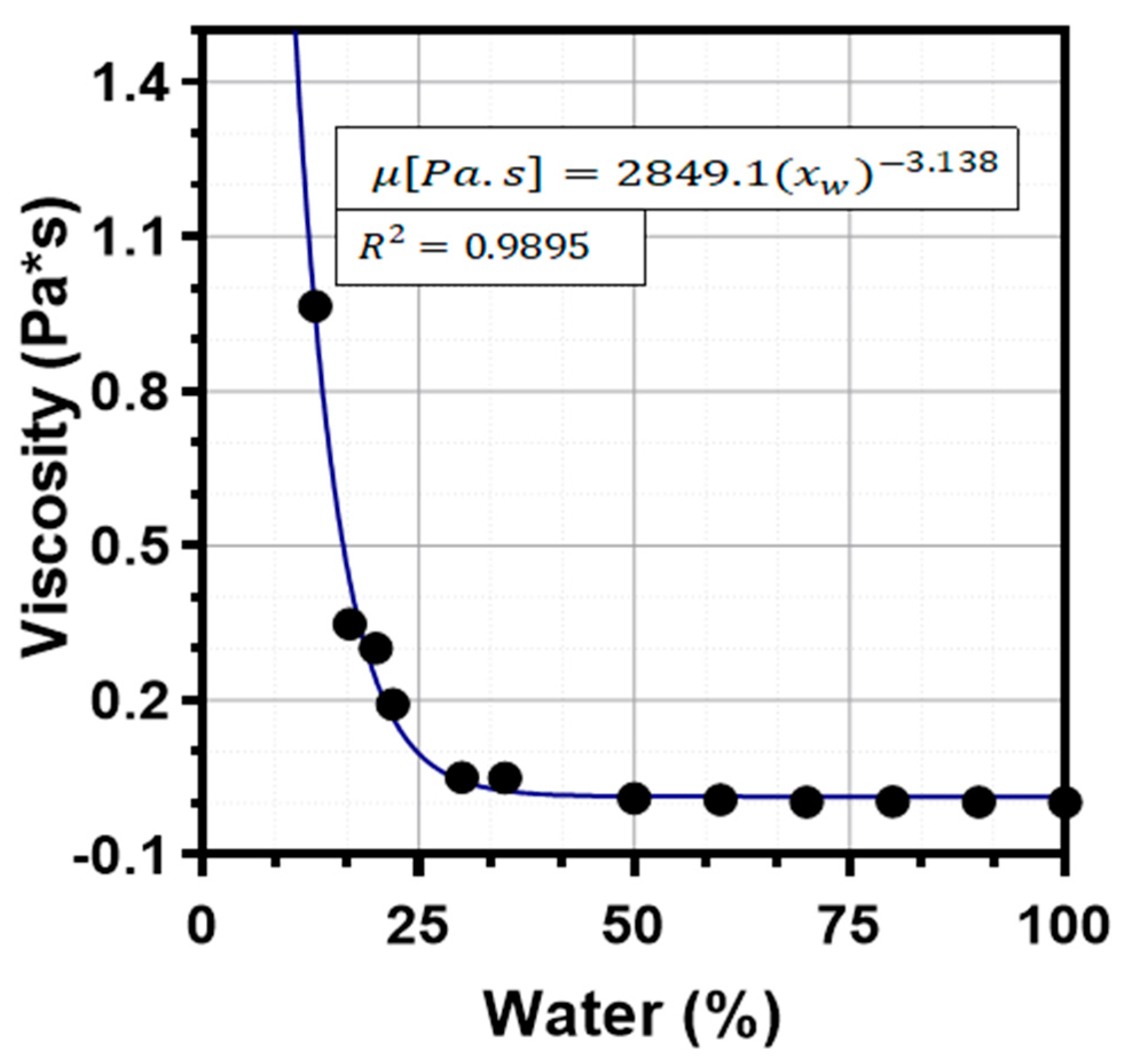
| Parameter | Viscosity (Pa·s) | Max Shear Stress (Pa) | Max Shear Rate (s−1) | Cell Concentration |
|---|---|---|---|---|
| EC | ||||
| SC | ||||
| CHO | ||||
| TN-368 | ||||
| SF-9 | ||||
| AG | ||||
| HeLa |
References
- Pérez, J.C.B.; Sánchez, R.A.H. Efecto de la relación agitación-aireación sobre el crecimiento celular y la producción de Azadiractina en cultivos celulares de Azadirachta indica A. Juss. Rev. Fac. Nac. Agron. 2010, 63, 5293–5305. [Google Scholar]
- Post, T. Understand the Real World of Mixing. AIChE J. FG-1 2010, 106, 25–32. [Google Scholar]
- Doran, P.M. Bioprocess Engineering Principles; Academic Press: Cambridge, MA, USA, 1995; ISBN 9780080528120. [Google Scholar]
- Ochoa, F.; Gomez, E. García- & Bioreactor scale-up and oxygen transfer rate in microbial processes: An overview. Biotechnol. Adv. 2009, 27, 103–226. [Google Scholar]
- Gogate, P.R.; Beenackers, A.A.C.M.; Pandit, A.B. Multiple-impeller systems with a special emphasis on bioreactors: A critical review. Biochem. Eng. J. 2000, 6, 109–144. [Google Scholar] [CrossRef]
- Buffo, M.M.; Corrêa, L.J.; Esperança, M.N.; Cruz, A.J.G.; Farinas, C.S.; Badino, A.C. Influence of dual-impeller type and configuration on oxygen transfer, power consumption, and shear rate in a stirred tank bioreactor. Biochem. Eng. J. 2016, 114, 130–139. [Google Scholar] [CrossRef]
- Uribe, A.R.; Rivera, R.; Aguilera, A.F.; Murrieta, E. Stirring and mixing. Enlace Químico 2012, 4, 22–30. [Google Scholar]
- Yunus, A.; Cimbala, J.M.; Sknarina, S.F. Mecánica de Fluidos: Fundamentos y Aplicaciones; Primera, Ed.; McGrawHill: New York, NY, USA, 2001; pp. 10–11. [Google Scholar] [CrossRef]
- Centeno Carrillo, J.; Maroto Centeno, J. Utilización de un frasco de Mariotte para el estudio experimental de la transición de régimen laminar a turbulento. Rev. Española Física 1999, 13, 42–47. [Google Scholar]
- Bird, R.B.; Stewart, W.E.; Lightfoot, E.N. Transport Phenomena, 2nd ed.; John Wiley & Sons: Hoboken, NJ, USA, 2006; ISBN 0470115394. [Google Scholar]
- Deen, W.M. Transport in turbulence flow. In Analysis of Transport Phenomena; Oxford University Press: New York, NY, USA, 1998; ISBN 0195084942. [Google Scholar]
- Chisti, Y.; Moo-Young, M. On the calculation of shear rate and apparent viscosity in airlift and bubble column bioreactors. Biotechnol. Bioeng. 1989, 34, 1391–1392. [Google Scholar] [CrossRef]
- Alfonsi, G. Reynolds-Averaged Navier-Stokes Equations for Turbulence Modeling. Appl. Mech. Rev. 2009, 62, 040802. [Google Scholar] [CrossRef]
- Proceedings of the STAR South East Asian Conference Best Practices Workshop: Heat Transfer, Singapore, 8–9 June 2015; p. 1.
- Hanjalić, K.; Popovac, M.; Hadžiabdić, M. A robust near-wall elliptic-relaxation eddy-viscosity turbulence model for CFD. Int. J. Heat Fluid Flow 2004, 25, 1047–1051. [Google Scholar] [CrossRef]
- Domen, J.; Jain, R.; Cui, Z. Chapter 4-Environmental Impacts of Mining. In Environmental Impact of Mining and Mineral Processing; Butterworth Heinemann: Oxford, UK, 2016; pp. 1–53. [Google Scholar]
- Collett, R.S.; Oduyemi, K. Air quality modelling: A technical review of mathematical approaches. Meteorol. Appl. 1997, 4, 235–246. [Google Scholar] [CrossRef]
- SIEMENS Using the Volume Of Fluid (VOF) Multiphase Model. Available online: http://mdx2.plm.automation.siemens.com/sites/default/files/Presentation/18% (accessed on 30 May 2020).
- Armenante, P.M.; Nagamine, E. Uehara Effect of Low Off-Bottom Impeller Clearance on the Minimum Agitation Speed for Complete Suspension in Stirred Tanks. Chem. Eng. Sci. 1998, 9, 1757–1775. [Google Scholar] [CrossRef]
- Eppendorf. AG New Brunswick BioFlo ® /CelliGen ® 115 Operating Manual; Eppendorf: Hamburg, Germany, 2012. [Google Scholar]
- Spanjers, H.; Olsson, G. Modelling of the dissolved oxygen probe response in the improvement of the performance of a continuous respiration meter. Water Res. 1992, 26, 945–954. [Google Scholar] [CrossRef]
- LabX New Brunswick Bioflo Reactors and Fermentors. Available online: https://www.labx.com/product/new-brunswick-bioflo-reactors-and-fermentors (accessed on 30 May 2020).
- Celik, I.; Chen, C.J.; Roache, P.J.; Scheurer, G.; Washington, D.C. Quantification of Uncertainty in Computational Fluid Dynamics. Eng. Div. Summer Meet. 1993. [Google Scholar]
- Eça, L.; Hoekstra, M. A procedure for the estimation of the numerical uncertainty of CFD calculations based on grid refinement studies. J. Comput. Phys. 2014, 262, 104–130. [Google Scholar] [CrossRef]
- Furukawa, H.; Kato, Y.; Inoue, Y.; Kato, T.; Tada, Y.; Hashimoto, S. Correlation of power consumption for several kinds of mixing impellers. Int. J. Chem. Eng. 2012, 2012, 1–6. [Google Scholar] [CrossRef] [Green Version]
- Spogis, N. Metodologia para determinação de curvas de potencia e fluxos caracteristicos para impelidores axiais, radiais e tangenciais utilizando a fluidodinamica computacional. Dissertation (master’s), Universidade Estadual de Campinas, Faculdade de Engenharia Quimica, Campinas, SP. 2002. Available online: http://www.repositorio.unicamp.br/handle/REPOSIP/266231 (accessed on 5 June 2020).
- Navisa, J.; Sravya, T.; Swetha, M.; Venkatesan, M. Effect of bubble size on aeration process. Asian J. Sci. Res. 2014, 7, 482–487. [Google Scholar] [CrossRef] [Green Version]
- Mcginnis, D.F.; Little, J.C. Predicting diffused-bubble oxygen transfer rate using the discrete-bubble model. Water Res. 2002, 36, 4627–4635. [Google Scholar] [CrossRef]
- Lange, H.; Taillandier, P.; Riba, J.-P. Effect of high shear stress on microbial viability. J. Chem. Technol. Biotechnol. 2001, 76, 501–505. [Google Scholar] [CrossRef]
- Keane, J.T.; Ryan, D.; Gray, P.P. Effect of shear stress on expression of a recombinant protein by Chinese hamster ovary cells. Biotechnol. Bioeng. 2003, 81, 211–220. [Google Scholar] [CrossRef]
- Iordan, A.; Duperray, A.; Verdier, C. Fractal approach to the rheology of concentrated cell suspensions. Phys. Rev. E 2008, 77, 11911. [Google Scholar] [CrossRef] [PubMed] [Green Version]
- Cai, M.; Zhang, Y.; Hu, W.; Shen, W.; Yu, Z.; Zhou, W.; Jiang, T.; Zhou, X.; Zhang, Y. Genetically shaping morphology of the filamentous fungus Aspergillus glaucus for production of antitumor polyketide aspergiolide A. Microb. Cell Fact. 2014, 13, 73. [Google Scholar] [CrossRef] [PubMed] [Green Version]
- Goldblum, S.; Bae, Y.K.; Hink, W.F.; Chalmers, J. Protective effect of methylcellulose and other polymers on insect cells subjected to laminar shear stress. Biotechnol. Prog. 1990, 6, 383–390. [Google Scholar] [CrossRef]
- Das, J.; Maji, S.; Agarwal, T.; Chakraborty, S.; Maiti, T.K. Hemodynamic shear stress induces protective autophagy in HeLa cells through lipid raft-mediated mechanotransduction. Clin. Exp. Metastasis 2018, 35, 135–148. [Google Scholar] [CrossRef] [PubMed]
- Chakraborty, S.; Nandi, S.; Bhattacharyya, K.; Mukherjee, S. Probing Viscosity of Co-Polymer Hydrogel and HeLa Cell Using Fluorescent Gold Nanoclusters: Fluorescence Correlation Spectroscopy and Anisotropy Decay. ChemPhysChem. 2020, 21, 406–414. [Google Scholar] [CrossRef] [PubMed]
- Karpinska Portela, A.M.; Bridgeman, J. Towards a robust CFD model for aeration tanks for sewage treatment–A lab-scale study. Eng. Appl. Comput. Fluid Mech. 2017, 11, 371–395. [Google Scholar] [CrossRef]
- Karpinska, A.M.; Bridgeman, J. CFD as a tool to optimize aeration tank design and operation. J. Environ. Eng. 2018, 144, 5017008. [Google Scholar] [CrossRef]


| Impeller Type | Diameter (cm) |
|---|---|
| Rushton | 6.09 |
| Paddles | 11.46 |
| Propeller | 10.40 |
| S. Propeller | 6.01 |
| Factors | Levels |
|---|---|
| Impeller type | Propeller |
| Rushton | |
| Paddles | |
| Small Propeller | |
| Airflow (L/min) | 2.5 |
| 5 | |
| Agitation velocity (RPM) | 100 |
| 200 |
| Parameter | Brunswick Bioflo/CelliGen 115 Bioreactor |
|---|---|
| Base Size (cm) | 2.55 |
| Relative target size (to base size) (%) | 10 |
| Relative minimum size (to base size) (%) | 10 |
| Relative prism layer total thickens (to base size) (%) | 10 |
| Number of prism layers | 4 |
| GCI Parameters | Value | |
|---|---|---|
| = Power | (%) | 3.98 |
| (%) | 4.85 | |
| 6.38 | ||
| = Shear rate | (%) | 0.66 |
| (%) | 0.27 | |
| 0.34 | ||
| Parameter | Brunswick Bioflo/CelliGen 115 Bioreactor |
|---|---|
| Mesh | Semi-fine |
| Number of Cells | 2.58 × 10⁶ |
| Angular Velocity (RPM) | 600 |
| Power (W) | 44.59 |
| Shear Rate (s−1) | 83.80 |
| Impeller | Run ID | ||||||
|---|---|---|---|---|---|---|---|
| Paddle | 5.0 | 100 | 1 | 0.0025 | 9 | 0.192 | 15.211 |
| Paddle | 5.0 | 250 | 2 | 0.0061 | 21.96 | 7.714 | 32.857 |
| Paddle | 2.5 | 100 | 3 | 0.0017 | 6.12 | 0.192 | 15.211 |
| Paddle | 2.5 | 250 | 4 | 0.0045 | 16.2 | 7.714 | 32.857 |
| Propeller | 5.0 | 100 | 5 | 0.0026 | 9.36 | 0.069 | 2.376 |
| Propeller | 5.0 | 250 | 6 | 0.0029 | 10.44 | 0.940 | 8.631 |
| Propeller | 2.5 | 100 | 7 | 0.0019 | 6.84 | 0.069 | 2.376 |
| Propeller | 2.5 | 250 | 8 | 0.0018 | 6.48 | 0.940 | 8.631 |
| Small Propeller | 5.0 | 100 | 9 | 0.0021 | 7.56 | 0.001 | 0.723 |
| Small Propeller | 5.0 | 250 | 10 | 0.0032 | 11.52 | 0.013 | 3.948 |
| Small Propeller | 2.5 | 100 | 11 | 0.0013 | 4.68 | 0.001 | 0.723 |
| Small Propeller | 2.5 | 250 | 12 | 0.0022 | 7.92 | 0.013 | 3.948 |
| Rushton | 5.0 | 100 | 13 | 0.0032 | 11.52 | 0.020 | 1.306 |
| Rushton | 5.0 | 250 | 14 | 0.0056 | 20.16 | 0.334 | 8.446 |
| Rushton | 2.5 | 100 | 15 | 0.0023 | 8.28 | 0.020 | 1.306 |
| Rushton | 2.5 | 250 | 16 | 0.0044 | 15.84 | 0.334 | 8.446 |
| Paddle–Propeller | 5.0 | 100 | 17 | 0.0032 | 11.52 | 0.178 | 13.659 |
| Paddle–Propeller (inv) | 5.0 | 100 | 18 | 0.0031 | 11.16 | 0.178 | 13.659 |
| Paddle–Propeller | 5.0 | 250 | 19 | 0.0062 | 22.32 | 2.869 | 37.119 |
| Paddle–Propeller (inv) | 5.0 | 250 | 20 | 0.0080 | 28.8 | 2.869 | 37.119 |
| Paddle–Propeller | 2.5 | 100 | 21 | 0.0019 | 6.84 | 0.178 | 13.659 |
| Paddle–Propeller | 2.5 | 250 | 22 | 0.0049 | 17.64 | 2.869 | 37.119 |
| Paddle–Rushton | 5.0 | 100 | 23 | 0.0034 | 12.24 | 0.231 | 14.968 |
| Paddle–Rushton (inv) | 5.0 | 100 | 24 | 0.0031 | 11.16 | 0.231 | 14.968 |
| Paddle–Rushton | 5.0 | 250 | 25 | 0.0056 | 20.16 | 3.702 | 41.458 |
| Paddle–Rushton (inv) | 5.0 | 250 | 26 | 0.0047 | 16.92 | 3.702 | 41.458 |
| Paddle–Rushton | 2.5 | 100 | 27 | 0.0020 | 7.2 | 0.231 | 14.968 |
| Paddle–Rushton | 2.5 | 250 | 28 | 0.0056 | 20.16 | 3.702 | 41.458 |
| Propeller–Rushton | 5.0 | 100 | 29 | 0.0030 | 10.8 | 0.069 | 3.727 |
| Propeller–Rushton (inv) | 5.0 | 100 | 30 | 0.0026 | 9.36 | 0.069 | 3.727 |
| Propeller–Rushton | 5.0 | 250 | 31 | 0.0028 | 10.08 | 1.111 | 13.792 |
| Propeller–Rushton (inv) | 5.0 | 250 | 32 | 0.0043 | 15.48 | 1.111 | 13.792 |
| Propeller–Rushton | 2.5 | 100 | 33 | 0.0018 | 6.48 | 0.069 | 3.727 |
| Propeller–Rushton | 2.5 | 250 | 34 | 0.0028 | 10.08 | 1.111 | 13.792 |
© 2020 by the authors. Licensee MDPI, Basel, Switzerland. This article is an open access article distributed under the terms and conditions of the Creative Commons Attribution (CC BY) license (http://creativecommons.org/licenses/by/4.0/).
Share and Cite
Ramírez, L.A.; Pérez, E.L.; García Díaz, C.; Camacho Luengas, D.A.; Ratkovich, N.; Reyes, L.H.
CFD and Experimental Characterization of a Bioreactor: Analysis via Power Curve, Flow Patterns and
Ramírez LA, Pérez EL, García Díaz C, Camacho Luengas DA, Ratkovich N, Reyes LH.
CFD and Experimental Characterization of a Bioreactor: Analysis via Power Curve, Flow Patterns and
Ramírez, Luis A., Edwar L. Pérez, Cesar García Díaz, Dumar Andrés Camacho Luengas, Nicolas Ratkovich, and Luis H. Reyes.
2020. "CFD and Experimental Characterization of a Bioreactor: Analysis via Power Curve, Flow Patterns and