Not Just Numbers: Mathematical Modelling and Its Contribution to Anaerobic Digestion Processes


School of Engineering, Newcastle University, Newcastle-upon-Tyne NE1 7RU, UK
Processes 2020, 8(8), 888; https://0-doi-org.brum.beds.ac.uk/10.3390/pr8080888
Submission received: 30 June 2020
/
Revised: 15 July 2020
/
Accepted: 21 July 2020
/
Published: 24 July 2020
(This article belongs to the Special Issue Modelling and Optimal Design of Complex Biological Systems)
Abstract
:Mathematical modelling of bioprocesses has a long and notable history, with eminent contributions from fields including microbiology, ecology, biophysics, chemistry, statistics, control theory and mathematical theory. This richness of ideas and breadth of concepts provide great motivation for inquisitive engineers and intrepid scientists to try their hand at modelling, and this collaboration of disciplines has also delivered significant milestones in the quality and application of models for both theoretical and practical interrogation of engineered biological systems. The focus of this review is the anaerobic digestion process, which, as a technology that has come in and out of fashion, remains a fundamental process for addressing the global climate emergency. Whether with conventional anaerobic digestion systems, biorefineries, or other anaerobic technologies, mathematical models are important tools that are used to design, monitor, control and optimise the process. Both highly structured, mechanistic models and data-driven approaches have been used extensively over half a decade, but recent advances in computational capacity, scientific understanding and diversity and quality of process data, presents an opportunity for the development of new modelling paradigms, augmentation of existing methods, or even incorporation of tools from other disciplines, to ensure that anaerobic digestion research can remain resilient and relevant in the face of emerging and future challenges.
1. Introduction
Mathematical modelling has an important and continued role to play in the design and operation of engineered biological systems (EBS), where the inherently complex interaction between biotic and abiotic components may result in unpredictable and undesirable process behaviour requiring operator intervention or advanced control architecture. Over the last four decades (circa 1980 onwards), much focus has been on the development and extension of classical models based on first-principles theory and engineering knowledge. Notably, the work of several research groups coalesced around a unified mechanistic model with the aim to represent, i.e. simulate, the dynamics of the activated sludge treatment process [1,2]. This reference model, the Activated Sludge Model No. 1 (ASM1) [3], initiated a highly productive period in wastewater engineering, where mathematical modelling became a distinct and important field within the bioprocess engineering community. Iterations of ASM1 to include phosphate accumulating organisms (ASM2 [4]) and subsequent consideration of their denitrifying ability (ASM2d [5]), facilitated a greater degree of granularity in the modelling of wastewater treatment processes. However, the increased model complexity due to additional requirements on parameterisation and model calibration highlighted the difficulty in developing rigorous mathematical models that are a trade-off between complexity and accuracy. Nevertheless, the framework of these models has remained in popular use, through refinement and augmentation, as the standard modelling tool used by wastewater engineering practitioners and researchers.
The focus of this review is the globally used anaerobic digestion (AD) process that conventionally transforms biodegradable organics (e.g., agricultural residues, food waste, wastewater treatment sludge) into energy-rich biomethane and nutrient-rich biosolids under anaerobic environmental conditions. While the standard process consists of four well-characterised conversion stages (hydrolysis → acidogenesis → acetogensis → methanogesis), the complexity that manifests in AD biochemistry, energetics, microbial diversity and process operation lends itself well to mathematical modelling, as will be explored here.
Given the relative ubiquity of the ASMs and a reawakening of AD research during the late 1990s, it was inevitable that engineers and scientists would seek to develop a similar modelling framework to facilitate dynamical interrogation of this net energy positive environmental technology. Building on the fundamental process kinetics and physico-chemistry of the ASMs, with some changes in reporting of units and use of kinetic rates, Anaerobic Digestion Model No. 1 (ADM1) [6] provided a valuable in silico tool to support an expanding field of academic research. ADM1 has remained the standard model in AD research and in its integration with ASM1 as the Benchmark Simulation Model No. 2 [7,8], has provided the ability for plant-wide modelling of wastewater treatment systems [9]. This process coupling extends the capacity of sub-component models for simulation, design and optimisation, to include whole plant Life Cycle Assessment [10], future-proofing the transition from conventional wastewater treatment plants to water resource recovery facilities [11,12], and the augmentation of novel processes and technologies [13,14].
ADM1 is known to have severe limitations. As with ASM1, it does not handle phosphorus and its associated biochemistry, nor does it consider sulphur and iron species or, until recently, the bioavailability of trace elements, which are important components for stable anaerobic digester operation. Extensions to the original model have subsequently addressed these omissions [15,16,17,18]. However, unlike the iterations of the ASMs, there has been no standardised progression of ADM1, but rather bespoke modifications and simplifications tailored towards process specific objectives [19,20], more efficient computation in engineering software [9,21], or the incorporation of new empirical knowledge and parameter data [22,23]. In their excellent 2015 review of AD modelling application and needs, Batstone et al. [22] state that up to that point, forming consensus towards the establishment of a standardised ADM2 is an attractive proposition, but establishment of both the science and underlying mechanics of the model remained transitory.
In this review, we revisit the origins of mathematical modelling for application to anaerobic digestion and comment on the current state-of-the-art with respect to the theory, applications, and technologies that comprise or exist alongside models for research and practice. In Section 2, we place the most widely known and used model, ADM1, in a wider historical context and discuss its relevance to current practice. Large, highly parameterised models have well-understood limitations and requirements for managing uncertainty. Although exponential increases in computational performance (cf. Moore’s Law) have significantly reduced the simulation time of complex and highly dimensional models, simplifying assumptions and lumping of parameters are often employed in mathematical models to aid study of anaerobic systems. However, in Section 3 we discuss the potential insights that reduced or minimal models, which often represent a sub-component of the larger process, can provide, particularly in combination with analytical tools common to a branch of mathematics known as dynamical systems theory. Deterministic modelling remains generally the standard in engineering practice. Although the use of data-driven models and machine learning for monitoring and control of biological systems has developed in a similar time-frame, it has largely remained under-used by the engineering community. In Section 4, the growth of digital tools and data modelling for application to anaerobic digestion is described and comment on the increasing need for making use of the increasingly diverse sources of data and meta-data that have potential to reveal process knowledge ex-situ and across process scales. In Section 5 we conclude by taking a wide-lens view of the future of mathematical modelling for anaerobic digestion, focusing on the role of models as anaerobic processes diversify and metabolic pathways are re-purposed for alternative energetic and chemical products.
Engineered anaerobic systems have a vital function for future energy security, and the use of mathematical models will continue to be important and much more intrinsic in plant design, operation and control. This review celebrates what has gone before and the increasing role that mathematical modelling plays in design, control, operation and analysis of engineered anaerobic systems (See Figure 1 for a chronological chart of published studies on AD modelling). The review provides some commentary on anticipated future trends, as greater empirical and theoretical knowledge becomes available for derivation of more representative and rigorous models, often by incorporating ideas employed more commonly in other fields. The review aims to be accessible to readers from a diverse background and, as such, we limit the use of mathematical equations to elementary examples that are qualified in the text. More thorough reviews of the mathematical derivations of the methods presented here are cited in the text.
2. A First-Principles, Engineering Approach to Modelling Anaerobic Digestion
The history of anaerobic digestion modelling from an engineering perspective, which is a mathematical description of the microbial dynamics and biochemical processes resulting in sequential biodegradation of complex organic material into biogas, begins over 50 years ago.
The pioneering work of John F. Andrews, an environmental engineer at Clemson University, South Carolina, formed the touchstone for incremental development of practical mathematical models that could be understood and used by both researchers and practitioners to augment their experimental studies. Andrews used the structural elements of Ordinary Differential Equations (ODEs), which had facilitated the dynamical study of microbiology using mathematical constructs by researchers such as Lotka, Volterra, Haldane, Monod, Rashevsky, the forefathers of a discipline now commonly referred to as mathematical biology [24]. It is interesting to note that these key players came from broad scientific disciplines; Haldane was a geneticist, Monod a biochemist, Volterra a mathematician, Lotka a biophysicist, and Rashevsky a theoretical physicist.
The early work by Andrews built on the empirical and theoretic research of these pioneers to derive mathematical expressions that were founded on first-principles chemistry encapsulated by the Michaelis-Menten enzymatic reaction rate Equation [25]
where is the rate of product formation, is the maximum achievable rate of the chemical system, is a constant representing the substrate concentration, , at a reaction rate half the . Through the early work of Lotka and Volterra, describing the dynamics of biological systems as a pair of non-linear ODEs (i.e., the predator-prey equations) (see, for example [26]), and the empirical rationalisation of the Michaelis-Menten equation by Jacques Monod to derive an equation for microbial growth on a rate-limiting nutrient [27], the platform for mathematical modelling of bioengineering systems was established [28]. Andrews synthesised this structural and empirical knowledge to describe microorganisms growing on substrates that are self-inhibitory above a threshold concentration (e.g., those found in industrial wastewater treatment such as ammonia, phenols, and volatile fatty acids). Andrews coupled the Haldane function describing enzymatic inhibition with the Monod equation for microbial growth to develop Lotka-Volterra type non-linear ODEs for simulating the continuous-culture dynamics of microorganisms under rate-limiting inhibition [29]
where are the microbial biomass concentrations in the reactor influent and effluent, respectively, are the substrate concentrations in the reactor influent and effluent, is the maximum specific growth rate, is the mean residence time in the reactor (Note. 1/ is commonly denoted as D, the dilution rate, in current modelling practice), is the half-saturation constant, is the inhibition constant, and Y is the yield coefficient of biomass growing on the substrate (for units, see original article [29]). What is notable about this study is that it is one of the first examples of the use of digital computing to obtain solutions to a system of equations describing microbial dynamics. A digital analogue simulation program, PACTOLUS, ran the model on an IBM360 computer, employing a circuit-like block-diagram approach more commonly associated with electronic engineering.
The importance of seminal work in the late 1960s and early 1970s by researchers such as Andrews and Perry L. McCarty, a pioneering environmental engineer whose work on AD kinetics and energetics resonates with engineers and modelers to this day, cannot be understated. They developed an empirically derived basis for coupling microbiology with engineering practice using mathematical tenets. Integral to this was the understanding that process stability, and ultimately failure (e.g., through organic overloading, product inhibition), could be predicted by appropriate kinetic models supported by experimental evidence. Andrews published the first mathematical model of the anaerobic digestion process in 1969 to address the increasing reports of digester failures [30]. Similarly, McCarty and his former PhD student, Lawrence, derived process models from observations from anaerobic continuous cultures to determine limits of operation based on kinetic theory [31,32]. Anaerobic digestion as an industrial process became prominent in Europe in response to energy shortages during World War II, and in the United States, anaerobic municipal solid waste treatment had existed as a technology from around the same period. Given the complexity of feedstocks that were being used in AD, and the relative immaturity in process engineering, the high prevalence of reactors experiencing process instability and failing would be significant. It was, therefore, serendipitous that Andrews initiated a first epoch in AD process modelling to understand stability just a few years before the 1973 OPEC oil embargo precipitated an oil crisis that directly led to a drive towards alternative energy supplies, with AD at the forefront.
The dynamic modelling approach was extended further to include a method to incorporate changes in pH through the introduction of phase (gas, liquid, biological) interactions and alkaline buffering capacity (i.e., CO—bicarbonate system) [33]. The time-dependent, predictive characteristics of this extended model provided the ability to obtain a semi-quantitative assessment of the model uncertainty, which is the difference between observed (experimental) data and model prediction for the model variables of interest. Noting that model uncertainty comprises parametric uncertainty and structural uncertainty, and both model inputs and experimental observations are subject to measurement uncertainty, then it is generally accepted that the model predictions are not a perfect representation of reality [34]. In turn, this acknowledgment of uncertainty laid the foundation for model-based process control of bioengineering systems such as the activated sludge process and anaerobic digestion [34,35,36,37,38]. This was a momentous leap-forward in the early days of programmatic computing, especially as industry and academia were starting to coalesce around methods for incorporation of Instrumentation, Control and Automation (ICA) technology for the improvement of biological treatment processes [39,40].
Over subsequent years, other research groups began to build on the work of Andrews and further extend AD models to include additional stages of the process beyond acetoclastic methanogensis, the focus of the earlier models [30,33]. Fundamentally, these later models adopt the same mass-balanced, reaction kinetics approach as Andrews, adding more processes and components to describe an increasingly more complex but also more complete conventional anaerobic digestion process. Hill and Barth included heterotrophic acidogens and the obligate methanogens previously studied by Andrews, and a function describing methanogen inhibition by Volatile Fatty Acids (VFA) and ammonia [41]. As with previous models, the authors considered only the acetate metabolic pathway based on existing empirical knowledge at the time. Notation in this model differs minimally from that provided by Andrews in Equations (2) and (3), with the dilution term () now given as the flow rate over the reactor volume () and the differential terms on the right-hand side stated implicitly.
A thorough mathematical description of the gas-liquid transfer of carbonate and ammonia, and the algebraic equations describing charge balancing to calculate temperature-corrected pH, is reported for the first time in this work. This detail invariably led to greater model complexity and, at the time, reliance on high specification computers and bespoke programming languages (Continuous modelling Simulation Program, CMSP, op. cit. Hill & Barth). Although the anaerobic digestion process was understood to be microbially diverse, process or population scale modelling could be simplified due to the highly structured and often compartmentalised nature of bioreactor systems. This structuring, based on agglomeration of microbial ecological functions, i.e., step-wise mass-balanced and stoichiometrically rational biochemical reactions performed by mixed but functionally distinct microorganisms, provided a firm basis from which mathematical modelling of biologically engineered systems became established in the following two decades. Table 1 indicates a selection of the key mathematical models that provided necessary iterations towards a consensus dynamic model for anaerobic digestion, manifest as the Activated Sludge Model No. 1. For brevity, the list is by no means exhaustive and does not aim to present any detailed analysis of the models, which may instead be found in comprehensive reviews elsewhere [42,43,44].
Modelling efforts were bolstered by research conducted in empirical microbiology, which contributed to providing better characterisation (i.e., parameterisation) of anaerobic growth kinetics and understanding of the metabolic and biochemistry of the principal reaction pathways [54,55,56,57]. Experimental work provided the data and knowledge to determine the structure and stoichiometric properties of the anaerobic digestion process that, in turn, allowed for an emerging formalism in parallel model development. An important body of work that motivated a structural approach to AD modelling was Gujer and Zehnder’s extensive study of anaerobic digestion conversion processes [55], which built on an earlier proposed structure describing overall substrate flux from particulate organic matter to methane and carbon dioxide end-products [58]. Their study describes anaerobic digestion as six distinct conversion processes, integrating established knowledge of the acetogenesis and methanogenesis steps with emerging bioprocess kinetics and microbial research on the mechanisms of organic matter hydrolysis and acidogenesis, thus providing a complete description of the canonical AD process as understood at that time. Defining the units of substrate flux in mass of theoretical Chemical Oxygen Demand (tCOD) as opposed to a molar basis, was a consideration replicated from activated sludge modelling, in its conventional use for measurement of wastewater characteristics and given its implicit function for calculating carbon oxidation states and, thus mass balancing of biochemical reactions [6,59]. Note. Typically, for anaerobic modelling, concentrations of organic compounds are given in units kgCOD m, and inorganic carbon and nitrogen in kmole m, whereas ASMs generally use mg L. The case for using molar units, however, was argued on the basis that the inclusion of inorganic carbon (CO) to close the mass balance for anaerobic oxidation of VFAs invalidates the stoichiometric carbon balance of the biochemical reactions [60].
The structured approach was further formalised by Bryers [48] using simple matrix algebra to derive expressions for the biological reactions in the form of a stoichiometric matrix of () molar coefficients (, for reactions and components [reactants, biomass, gases]) to ensure a completely mass-balanced system of process equations. In considering a unit basis of mass COD, normalised yield coefficients defining consumed (−) or formed (+) in the ith reaction are given by
where and are the molecular weight and COD mass equivalence of component , respectively, and indicates the limiting reactant in the ith reaction. Now, using matrix algebra, we have the following condition under the principle of mass conservation
where Y is an matrix of yield coefficients and S is a vector of length n of components.
The use of a structural matrix for deriving a system of equations representing biochemical reactions was first proposed by Petersen [61] and employed in the development of a mathematical model of activated sludge systems by the IAWPRC (now International Water Association, IWA) Task Group on Mathematical modelling for Design and Operation of Biological Wastewater Treatment [3]. The Gujer matrix, as schematically summarised in Figure 2, is partitioned into three sections comprising a matrix of stoichiometric coefficients and a process rate vector, as described above, and a composition matrix that includes conservative constituents of the state variables, e.g., biomass contains both COD and nitrogen, which ensure proper mass and charge balancing as model resolution increases, i.e., the product of each row in and each row in the composition matrix will be zero.
The conversion rates for each state variable can be simply calculated by the column-wise summation of the product of stoichiometric terms and process rates
where is the matrix of stoichiometric terms and is a vector of n process specific kinetic rates, which take the form
where is the substrate-limited growth rate of organism X, defined by some growth function (e.g., Monod saturating kinetics, Contois density dependent growth, etc.), cf. the final term in Equation (3). Note. Hydrolysis in these early models is typically included as a first-order reaction rate (i.e., ). The notation , is used to indicate that the resultant vector of rates are time-dependent and equivalent to a system of ODEs, with additional terms to mass balance the reactor and describe any liquid-gas transfer, which can be integrated to give transient dynamics of the process with respect to each state variable.
This highly structured matrix formulation for constructing biochemical reaction models was adopted as standard within the engineering community, leading to a general framework for modelling the activated sludge process, specifically related to nitrogen removal (ASM1) [3]). It was particularly open to integration in simulation software, especially programs with superior abilities for rapidly solving matrix linear algebra problems, such as Matlab and FORTRAN. Naturally, this led to several bespoke simulation software to provide engineers with the tools to rapidly develop and interrogate the models through process simulation, often in a modular way (e.g., Biowin, STOAT, GPS-X, SIMBA, AQUASIM) [1]. Although the Anaerobic Digestion Model No. 1 was published over ten years after the first ASM, work on developing a general anaerobic digestion model employing a similar structural and notational form emerged earlier. Siegrist et al. used a Gujer matrix of 14 processes and 18 state variables to model the digestion of mesophilic sewage sludge [52] and Christ et al. used this approach with a better description of the hydrolysis constants for the digestion of municipal organic residues [62]. Other groups incorporated greater degrees of resolution in existing deterministic models of the process, for example by separation of the complex organic substrates (carbohydrates and proteins) for hydrolysis [51,63,64].
The Anaerobic Digestion Model No. 1, developed by the IWA Task Group for Mathematical modelling of Anaerobic Digestion Processes [6], consolidates much of the preceding theory, empirical knowledge and mathematical structure referenced in this section. The original model represents a comprehensive five-stage anaerobic digestion process (including an initial disintegration step), with 19 sub-processes, comprising biochemical reactions (defined through the use of the Gujer matrix) incorporating degradable substrates and soluble/insoluble inerts, and physico-chemical reactions (non-biologically mediated processes such as ion association/disassociation, phase transfer). Biochemical processes are (1) an initial disintegration of composite material (e.g., lysed biomass) to particulates, which undergo (2) enzymatic hydrolysis (forming carbohydrates, proteins and lipids), (3) acidogenesis of simple sugars and amino acids to organic acids, CO and H, (4) acetogenesis of long-chain fatty acids and organic acids (butyrate, valerate, propionate) to acetate and hydrogen, and finally (5) acetoclastic and hydrogenotrophic methanogenesis. The model may be solved as a system of 32 ODEs, where some lumped variables are decoupled (e.g., inorganic carbon ). Biochemical reactions are assumed to follow the 1st-order rate law for extra-cellular processes and Monod-type substrate uptake for intra-cellular kinetics. Alternatively, the model can be defined as a system of Differential Algebraic Equations (DAE), with the biochemical reactions integrated explicitly as a system of 26 ODEs (7 groups of bacteria and archaea, 19 catalysing processes), three liquid phase physico-chemical processes, and eight implicit algebraic variables (per reactor). This approach is a means to overcome the inherent ‘stiffness’ problem due to the fast hydrogen and pH dynamics (now explicitly calculated algebraically), which results in some numerical solvers encountering difficulty in solving the system of ODEs.
As noted earlier, the model is far from perfect but its flexibility and structure means it is suitable as a tool to be used at the design stage of AD plant development, for qualitative scenario testing, or for benchmarking control schemes [65,66,67]. As with the ASMs, modifications to the model have been implemented based on process requirements, such as operating mode [68,69], or to include new biochemical processes [70,71]. A more comprehensive transition to a consensus ADM No. 2 that addresses the main issues with the original model has yet to emerge, perhaps due to the lack of clear consensus or motivation, or that its inherent structure provides ample opportunity for modification of components for bespoke applications. Many of the suggested approaches relate to the lack of identifiability and heavy parameterisation of ADM1, which makes its use for process monitoring and model-based control difficult [72]. It is interesting to note that models that have sought to overcome the structural verbosity are greatly simplified, relying on fewer state variables and lumping parameters where practical. These models, such as the widely studied Bernard model (sometimes referred to as AMOCO or AM2) [73] and its subsequent mathematical treatments [43,74,75,76], relate back to the pioneering early work of Andrews and Graef, allow the process to be identifiable and enable process control schemes to be designed for improved or optimal process performance. Given the substantial quantity of literature on the topic of model identifiability, i.e., model selection and parameterisation, we refer the readers to an excellent review of the subject related to anaerobic digestion [77].
In the next section, we take a closer look at how reduced modelling approaches and their mathematical analysis are being used to provide further insights into the dynamic and steady-state behaviour of anaerobic digestion.
3. Reduced-Order Models Unlock the Power of Mathematics
It is common practice in modelling to start with a simple description of the system under investigation before building in complexity to achieve a more complete representation of reality. However, it should be noted that greater complexity does not necessarily equate to a higher degree of accuracy [78]. Terminology such as simplicity and complexity are often abstract and subjective, but in the frame of engineering models such as those discussed here, models with a greater number of parameters, state variables (dimension), and processes, or those that are highly non-linear, can be defined as complex. In mathematical sciences, this complexity is often referred to as model order and is the principle driver for the richness of dynamical behaviours captured in microbial community models [79].
The early anaerobic digestion models were low-order and aggregated, developed with the empirical knowledge of the biochemical reactions at that time, and constrained by the available computing resources and numerical solvers for integrating the system of differential equations. The dramatic advances in computational power and efficiency have provided engineers with an ever-increasing ability to simulate bioprocesses at greater levels of complexity and speed. However, there are still significant trade-offs between model resolution, accuracy and performance. For example, consider a mathematical model describing biofilm growth in a biological reactor. There are several approaches that can be taken to represent the evolution of this process in time, where the simplest would be to assume a homogeneous, quasi steady-state biofilm and to develop a model as a system of ODEs, for which the solution is trivial (e.g., [80]). The underlying assumption of a completely mixed system is not correct in practice, as biofilms are subject to diffusive mass transfer limitation, requiring consideration of spatial heterogeneity. Describing biofilm processes at higher dimensions, using Partial Differential Equations (PDEs) to solve the diffusion-limited mass transfer of biomass, gas and liquid (i.e., using the second-order Navier–Stokes equations or via the simpler boundary layer approximation), is non-trivial and significantly increases the computational requirements to find solutions [81]. A trade-off between model complexity and empirical uncertainty, which is the extent and accuracy of data to support model parameterisation, is one of the fundamental challenges that limits anaerobic digestion modelling [82].
Model order reduction methods such as decomposition, interpolation, low-order approximation and simplifying physics, are generally applied in engineering when high order models are computationally costly, or simulation become impractical. In EBS, mathematical biologists are often interested in the qualitative behaviour of the system rather than quantitative predictions, and the simpler models often allow for a tractable and complete analysis using techniques re-purposed from dynamical systems theory. It is important to ensure that the simplifying process retains conservation of the properties of the full-order model and has a low approximation error, otherwise analysis of the simple model becomes a study of a largely theoretical system with no further insight into the actual system. Anaerobic digestion is an ideal process for reduced-order modelling as it is highly compartmentalised allowing for easy decoupling of system interactions into smaller sub-processes with fewer state variables and parameters. Physico-chemical processes that may operate at significantly different timescales to the biochemical reactions may also be excluded.
The work of Andrews and colleagues (see Section 2) laid the early foundations for the application of dynamical analysis to anaerobic systems. They presented not only a template for mathematical modelling and dynamic simulation of the process, but were the first to discuss the opportunities for automatic process control to address system instability or failure caused by acidification or functional inhibition [33,36]. The analysis at this time involved exhaustive and time-consuming numerical simulation (by today’s standards) of a model over hundreds of operating points and process conditions. Although ADM1 consolidated state-of-the-art modelling and provided a reliable, if imperfect, representation of the process, others drew on these earlier ideas to address specific challenges such as the effect of reactor start-up conditions on process stability [83] and reactor control under process disturbances [84] or shock loading events [85,86].
A major benefit of with representative and qualitatively reliable reduced models, which are tractable to mathematical interrogation, is their availability for deeper study of the non-linear dynamics and the implications on system performance. In effect, they represent in silico tools that can complement time-consuming experimental studies, allowing for rapid investigation of local and global system behaviour to aid process or experimental design, derive new knowledge and understanding, and even suggest new operating protocols. It must be reiterated that models cannot completely replace practical experiments, nor prove comprehensively the underlying process mechanisms in all but the simplest of systems [87].
Anaerobic digestion models have been extensively studied by mathematical biologists due to their generally reducible structure, the rich dynamics emerging from relatively few biotic interactions, and the modularity of components facilitating an array of hypothesis driven studies. Mathematical analysis provides an ability to study the asymptotic behaviour of dynamical systems, such as AD, i.e., we are able to observe whether the process tends to some steady-state (stable equilibrium) or undergo unforced cycling (functional periodicity), for a given set of parameters and initial conditions of the process [88].
Several mathematical analyses of existing AD models appeared in the 2000s. The Bernard model (see Section 2), describes a two-step (acidogenesis-methanogenesis) process and is tractable to dynamical systems analysis of its steady-state behaviour and stability. One of the principal benefits of simpler models are their availability for model-based process control, where a perfect representation of the typically non-linear system is not required [89]. An initial bifurcation analysis of the model at equilibrium allows for identification of the key process variables that can significantly impact process behaviour and, thus, determine the main candidates for control variables and their critical values. Rincón et al. employed the model to design an adaptive controller to avoid biomass washout in an anaerobic digester through identification of the normal form bifurcation (i.e., local behaviour around the system equilibrium) with dilution rate as the bifurcating parameter [90]. An analytical determination of the model equilibria and their stability using general growth functions (i.e., only the functional response and not the mathematical structure of biomass growth is assumed), showed the existence of bistability dependent on initial conditions, where the process may converge to the nominal (desired) operating point or undergo acidification and complete washout of the biomass [74]. Recently, the Bernard Model was again used, and a rigorous analytical approach employed for open-loop control of Biochemical Oxygen Demand (BOD) within a target design interval [91]. The model has also been used to investigate the correct determination of overloading tolerance, defined as the distance between a stable interior equilibrium and the limit point of the system, for correct process monitoring [75,92]. To address issues of process representation with this reduced-order model, especially at low microbial population sizes, a stochastic process has been suggested as a way to account for its structural and parametric uncertainty [93], demonstrating a promising, if not fully realised, potential.
Researchers have studied the dynamical behaviour of EBS more generally [94], analysing the role of ecological interactions (e.g., competition, mutualism), rather than the specific process, on the existence, uniqueness and stability of the system [95,96,97]. These methods have also been applied to specific processes, such as the ammonia removal (SHARON) process [98], Anammox systems [99], anaerobic chlorophenol mineralisation [100,101], and conventional anaerobic digestion [102,103].
Although global stability analysis is challenging for models of increasing order, an initial numerical analysis of the full ADM1 (44 state variables, 29 ODEs, 15 DAEs) was achieved using a prediction-correction continuation algorithm for solving the differential equations and the Newton-Raphson method for simultaneous solution of the algebraic equations [104]. They showed, through performing a one-parameter bifurcation that a limit point exists when either the dilution rate increases, or substrate inlet concentration increases above or decreases below critical threshold values. A positive feedback loop between acetic acid accumulation and acetate degrader washout due to inhibition was identified as the critical mechanism in all three cases. Interestingly, a reduced model that allowed for the derivation of analytical solutions matched the qualitative behaviour of the full ADM1, as long as key features (i.e., ammonia inhibition) are preserved in the simpler model). Further study of the Börnhoft model have shown the role of inhibition on multiplicity of equilibria [105], expanded knowledge of the richness of AD dynamics, and counter-intuitive result suggesting biogas production may not always be optimal at the co-existence equilibrium [106]. A recent study not only provides new theoretical results for the model but examines the effects of stochasticity to account for both environmental and parameter uncertainty (as with [93] and the Bernard Model). Interestingly, the author’s find that the process is more prone to failure at start-up and becomes resilient to stochastic effects as the microbial communities establish. This is perhaps an intuitive result given real-world examples of start-up failure in biological reactors, for example due to acclimation issues (e.g., [107]).
A relatively simple example of bifurcation analysis, for illustrative purposes, is provided in Appendix A, using the model first developed by Andrews (See Section 2) [29].
Despite a significant body of work demonstrating the power of mathematical analysis for enhancing AD process understanding and enabling practical controller design, there still remains a substantial barrier to the wider use of these techniques for engineering purposes. In part this is due to a dissonance between the level of mathematical acuity required to conduct the analysis and the substantial process knowledge in the domain of engineers and scientists. Although there do exist groups who have core competency in both fields, more formal engagement through communication, collaboration and bottom-up empirical studies to support theoretical observations, will be necessary if it is to gain traction in the wider EBS community.
4. Empiricism, Data and the Digital Future
It may be argued that the mechanics of anaerobic digestion is well-understood, and the maturity of phenomenological models facilitate their use for process design, operation and control. In data poor environments, where measurements are infrequent, erroneous or hard to obtain, mechanistic models are an obvious choice. Nevertheless, improvement in sensor technology and fast and cheap tools to characterise the microbial communities in digesters through multi-omic analyses, has gifted scientists and engineers with a wealth of data and knowledge of their ecology [108,109,110]. When used effectively, this can provide a greater resolution of understanding, helping to derive models that link microbial community composition and function effectively [111,112]. For example, metagenomic data as microbial biomarkers have recently been used in combination with a data-driven model for prediction of ammonia and phenol inhibition [113].
Unlike data-rich industries that employ extensive process monitoring, there is a sense that data-driven models for systems that are open to high levels of uncertainty and transient or irregular variation in their operation is under-exploited. Although process monitoring and automatic control have become standard, for example in largest wastewater treatment systems, there is still a tendency to rely heavily on existing knowledge and empirically driven decision-making, where the plant operators are the experts, while much of the data gathered at the plant is unused. This has come to be known as ‘dark data’, which is data collected by an industry that is either archived or discarded in lieu of capacity or motivation for its use at that time [114]. It can be argued that for AD plants, dark data is largely irrelevant given the quantity of data typically acquired, but as industries are increasingly integrated, relying on automation and knowledge extracted from data, so the opportunities offered by digital technologies, which can manage large and diverse amounts of information, become apparent [115].
Machine learning and intelligent systems (i.e., Artificial intelligence, AI) have become, seemingly, pervasive in industry and society in general. However, there are risks associated with their wholesale adoption, and not because they threaten to break Asimov’s three laws of robotics, as popular media may like to imagine. The main issues for concern, especially in motivating uptake by the water and AD industries, are (i) the potential for application redundancy by using ‘smart’ tools that provide little or no benefit where conventional engineering practice is more than adequate (human vs. machine expertise), (ii) hastily appropriated technologies without undertaking due diligence on model relevance/adequacy or consideration of the long-term system behaviour (garbage in, garbage out/inherent non-linearity and uncertain dynamics), (iii) advanced models and algorithms may require significant cost and expertise to implement and maintain. Nevertheless, it is apparent that developments in data acquisition and computing capacity facilitates the cautious use of ‘smart models’ for improvement of EBS. Indeed, many of the tools used now are based on fundamental theory developed over a century of statistical and mathematical research. For example, popular dimension reduction and regression techniques such as Principal Component Analysis (PCA) and Partial Least Squares (PLS) have been re-purposed for chemometric process monitoring [116,117] and control [118] of anaerobic digesters. These multivariate methods are used to transform high-dimensional data by matrix factorisation into a lower-dimensional space that retains the maximal information (variance) present in the original dataset (X for PCA) or maximal covariance between predictor and response datasets (X and Y for PLS). The relationship between the original variables and samples projected into this reduced-dimensional space represents a model of the system or process described by the original data
where T and U are the projections (or scores matrices) of X and Y, respectively, P and Q are the weights (or loadings matrices). E and F are the residual matrices. If the purpose of these models is for process monitoring and fault or disturbance detection, it is vital that the data used to construct them, and the number of principal components (factors in PLS) to retain (, where , where m is the original number of variables in the X-block), represent its normal operating behaviour. New data acquired from the process is projected into the model and statistical measures (e.g., Hotelling’s T statistic) are used to identify samples that exceed some pre-determined threshold. The presumption is that these points represents non-normal process behaviour where variable contributions to the loadings may be examined to determine the source(s) of this exception.
PCA has been used as a data pre-processing step for extracting the correlation structure between variables. This variable selection method has been used as a preliminary step in the use of machine learning models to predict biogas yield from municipal AD [119]. A PCA model was used to detect disturbances in a sewage sludge fed AD process using PLS regression to chemical composition of the digestate from Near Infrared spectral data [120].
However, conventional multivariate models are limited by their stationarity [121], i.e., the model is a representation of the process over a fixed domain (e.g., time). To be useful for monitoring of dynamic processes, such as wastewater treatment and AD, adaptive/recursive methods have been developed for real-time monitoring and multivariate statistical process control, whereby the data model is updated with new information as it is acquired [122,123,124].
Unlike PCA, regression models, such as PLS, can be used to relate empirically derived data (measured explanatory variables) such as spectral data to one or more dependent (predicted) variables such as chemical concentrations, through their covariance structure. These regression models become useful in process operation when key performance indicators or control variables are difficult to measure. A model may be developed based on available and reliable measurements that are correlated with the target variable, acting as a soft-sensor for process monitoring and control. Like PCA methods, issues such as stationarity, multi-collinearity, and bias persist with ordinary PLS (OPLS). Robust method adaptations and rigorous data handling protocols are generally available (and required) to handle issues that may be encountered when using multivariate tools in practice [125,126]. Multivariate soft-sensors have been used quite widely by the wastewater community but fewer examples relating to the anaerobic digestion process have appeared [117,127,128]. This may be reflective of the general preference for using mechanistic models in AD or, anecdotally, the suspicion by practitioners that data-driven models are intangible and unrepresentative of the process. This may be exacerbated by the varied quality and quantity of data historically recorded at the plants themselves.
Nevertheless, ‘smart’ AD systems as a sub-class of a wider smartening of industry through the so-called 4th Industrial Revolution is an interesting and potentially valuable direction that practitioners may explore. This is especially pertinent in relation to the larger ‘Smart Water’ initiatives and repurposing of AD technology in bio-based manufacturing and biorefineries.
A renewed interest in Artificial Neural Networks (ANN) and Fuzzy logic, methods that have a long association with the bioprocessing and manufacturing industries, as well as AD itself [129,130], may propagate research and debate on the role of advanced data-driven models for application to AD moving forward. However, at present most applications of machine learning models have focused on conventional purposes, such as methane prediction [131,132,133].
In the final section we discuss how modelling is evolving by incorporation of interdisciplinary ideas and methods and show that no single approach is a catch all for engineered biological systems and anaerobic digestion, specifically.
5. Multi-Disciplinarity and the Future of Anaerobic Digestion Modelling
Mathematical modelling will play an increasingly important role in the design, monitoring and optimisation of EBS such as anaerobic digestion. As new challenges and opportunities emerge, technology develops and understanding increases, models will adapt and integrate the new knowledge acquired in the pursuit of smarter, cleaner and transformative processes. A recent review has highlighted possible trajectories for mathematical modelling of AD systems, both vertically (i.e., scale of models and connections across these scales) and horizontally (i.e., integration of processes, new anaerobic technologies) [22].
5.1. Hybrid Models
In the previous sections we have seen how disparate modelling approaches have been employed in the design, monitoring and control of AD. The selection of the appropriate model to use is dependent on its purpose, the quality, quantity and type of available process knowledge and data, the cost of model development and implementation versus the benefit of employing a model, among other considerations. It is a truism to state that no model is perfect, and often no single model is uniquely suited to the task in hand. For example, when there is lack of confidence in process measurements or data for characterising a process is unobtainable but a good mechanistic understanding has accrued, then a first-principles model seems logical. On the other hand, for many complex biological systems, only surface understanding of the system is known, and no consensus exists on the precise structural properties and interaction mechanisms, then a data-driven approach may be suitable. There is still debate, intensified by the current digitalisation epoch, as to whether machine learning is ready to entirely replace mechanistic modelling. As previously alluded to, the rapid adoption of AI and machine learning tools across many industries brings to mind the gold rush era. Some may succeed and prosper, while others may inevitably discover only fool’s gold. This is exemplified in the medical field, where early adoption of machine learning by clinicians is superseded by their acquisition in tackling more complex problems found in cell biology research. To quote a recent polemical opinion on this subject [134]:
Fundamental biology should not choose between small-scale mechanistic understanding and large-scale prediction. It should embrace the complementary strengths of mechanistic modelling and machine learning approaches …
Hybrid modelling is not a new concept, in fact many applications of what would be considered ‘pure modelling’ are a combination of structured and unstructured methods, e.g., consider parameter estimation techniques, such as the Extended Kalman Filter for fitting mechanistic models. However, explicit use of distinct modelling approaches has rarely been considered for application to bioprocesses. For anaerobic digestion, it appears viable that combining mechanistic and data-driven methods, together with extant process knowledge and empirical data would provide a means to overcome some of the shortcomings of either modelling approach alone [132].
An early example of hybrid modelling for AD employed a neural network to model process kinetics in combination with the Bernard Model described in Section 3 to ensure the ANN is constrained by the law of mass conservation (see Equation (5)) [135]. A similar approach using a kinetic model for lignocellulose fermentation and a PLS soft-sensor showed reasonable prediction potential over long time horizons [136]. The study is notable in its claim that it represents a simple demonstration of the digital twin concept. Although we do not discuss digital twins in this review, the concept that physical systems from individual process units to whole cities may be replicated digitally is becoming fairly ubiquitous, in tandem with concepts such as Industry 4.0 mentioned previously. Although it could be argued the use of buzzwords may attract attention to otherwise conventional research, all models may be classed as digital representations of real-world phenomena and some of these will feature in the establishment of digital twins in the future.
A neural network was used to predict AD performance and a Particle Swarm optimisation (PSO) algorithm is used to maximise methane yield, essentially employing a (meta)heuristic approach to evaluate a fitness function until a stopping criterion is reached (based on temperature and Volatile Suspended Solids (VSS), in this case) [137]. Nature-based methods, such as PSO, are not covered in this review, but more information on their emerging relevance to bioprocess monitoring, can be found in [138]. PCA was used as a feature extraction method to greatly reduce the dimensionality of ADM1 with relatively low loss of information, producing an identifiable model for supervisory control and optimisation of a winery effluent treatment plant [139]. A novel hybrid approach, augmenting ADM1 with information at the cellular level including intra-cellular fluxes and microbial activity, has recently been described. Flux Balance Analysis (FBA), a method to predict metabolic function from genomic information, was used to replace the Monod growth function in the ADM1 with an FBA growth prediction based on intra-cellular flux of metabolites [140]. The method allows for the dynamic prediction of optimal microbial composition, where conventional FBA provides steady-state analysis.
5.2. Thermodynamic Modelling
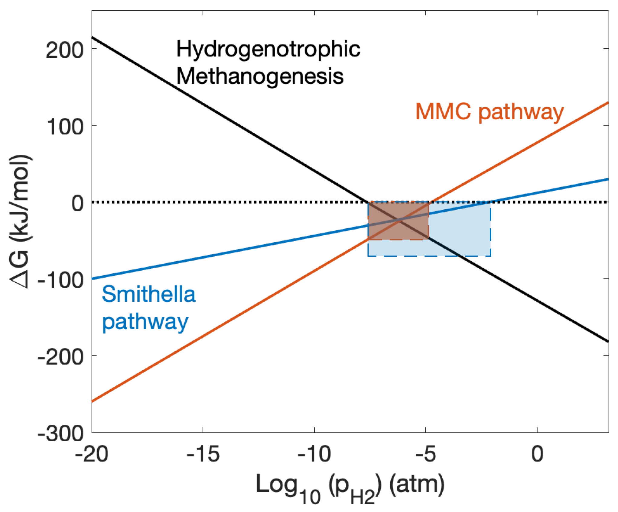
There has been considerable debate within the scientific community on the aptitude of purely kinetic models to describe the behaviour of systems that are subject to energetic constraints [28], especially in systems where microbial growth is directly linked to free energy availability. In anaerobic digestion, omission of energetic considerations in the mathematical description of the process dynamics will lead to qualitative and quantitative errors in model predictions, significantly undermining their usefulness. Indeed, the interplay between microbial kinetics and energetic constraints becomes important when the system approaches thermodynamic equilibrium, i.e., moving from exergonic sufficiency (net release of free energy) towards an endergonic state (net absorption of free energy) where biochemical reactions are completely inhibited (See Figure 3 for an example of the impact of hydrogen on thermodynamic inhibition of anaerobic propionate degradation). The rich microbial ecology that emerges in low energy environments, where thermodynamic inhibition is likely to constrain metabolic conversion, is both of interest and importance in the preservation of viable communities in AD [141,142] and the study of thermodynamic principles in biological systems has been an active area of research for decades [143]. Indeed, McCarty’s formative description of microbial growth energetics as the relationship of free energy of catabolism and the energy necessary for cell synthesis, the cell growth yield [144,145], is perhaps as important today as Andrews’ early conceptualisation of kinetic models for AD has been in the development of model formalisms for process control and optimisation over the last 20 years.
Various strategies have been proposed for the incorporation of thermodynamics into existing kinetic models or for the development of a universal theory. The Monod growth function is purely an empirical construct. Despite showing that the equation can relate with thermodynamic principles through the substrate affinity constant, i.e., [146], it is done so by making the assumption that only the limiting substrate and not microbial concentrations impact the growth dynamics. The Gibbs free energy change as the thermodynamic driving force for biochemical reactions forward was first coupled with a Michaelis-Menten type irreversible kinetic model describing anaerobic propionate degradation by Hoh and Cord-Ruwisch [147]. They surmised that reactions occurring close to thermodynamic equilibrium are reversible, driven by bidirectional reaction rates for the enzymatic conversion of substrates () to products (), and the reverse [25,148], given by the Briggs-Haldane mechanism
where E is the enzyme concentration, E is the enzyme-substrate-product complex, and , , and are the forward () and reverse () rate constants, which are combined to give the overall equilibrium constant . Under substrate saturation conditions, the Haldane kinetic scheme (shown in Equations (2) and (3), within square brackets) dominates any thermodynamic constraints. However, as the substrate is consumed, a trade-off between kinetics and thermodynamics becomes apparent [141], and a rate equation for the reversible reaction can be derived
where , is the mass-action ratio () at dynamic equilibrium). Given that the overall free energy change of reaction [149], then the general model proposed becomes [147]
In modelling the growth rate using the theory of reversible enzymatics, the energy required for driving the reaction and invested in maintaining other cellular functions not related to growth is overlooked, i.e., energy used for microbial growth is not the maximum free energy available in the system [150,151,152]. There has been significant developments in the understanding of thermodynamic principles for general application to microbial life, notably refinements in the derivation of metabolic energy requirements [153,154] and attempts to develop general or universal models to address shortcomings in established models, e.g., limits on metabolic parameter identification [155], and even the use of Maxwell-Boltzmann statistical physics to derive a fundamental link between microbial growth and energy states at the molecular level of substrates (i.e., the Microbial Transition State) [156,157].
However, despite a considerable amount of research on the application of thermodynamics to microbial systems, there are relatively few examples of direct application to the anaerobic digestion process itself. Oh and Martin used principles of thermodynamic equilibrium with chemical activity and fugacity together with a stoichiometric model to study energetic requirements of methanogensis [158], and recently Delattre et al. have proposed a kinetic-thermodynamic model to characterise a synthetic anaerobic tri-culture community performing sulphate reduction and methanogenesis [159]. Despite this, it is certain that as more consistent approaches are developed and theory more widely understood, appropriate thermodynamic models will be developed and tested for application to AD systems with the aim to improve performance and understand energetic limitations of different metabolic pathways. A recent paper has demonstrated that potentially, analytical methods from mathematics (see Section 3) can be used, despite the increased complexity, to elucidate the role of thermodynamics in biological growth models [160].
The thermodynamics of anaerobic digestion is inherently linked to the function of microbial communities and its inclusion in mathematical models has been shown to better predict inhibition of microbial growth under non-saturated substrate concentrations. Furthermore, there is an emerging trend for end-product diversification in AD systems, such as sustainable biorefineries producing high-value bio-based products [161,162,163]. The control and optimisation of these ‘manufacturing’ facilities will require models that represent metabolic pathway diversity and selection, especially the reversibility of novel catabolic pathways, through a general and robust framework describing the thermodynamic-kinetic trade-offs [142,152]. We anticipate significant integration of thermodynamic approaches with conventional engineering practice and microbial ecology in the coming years.
5.3. Computational Fluid Dynamics
Although ADM1 may be regarded as the most complete phenomenological description of the AD process from a bioprocess perspective, where the conditions of microbial growth are rigorously defined, there is an underlying assumption, as in many chemostat-type models, of spatial homogeneity, i.e., a completely mixed environment, or zero spatial dimensionality. This makes calculation of mass retention time and transfer rates relatively straightforward. However, in practice these ideal conditions are not observed and, at full-scale, the heterogeneous distribution of metabolites and biomass can lead to sub-optimal performance, dead-zones and unwanted reactor behaviour (e.g., foaming, physico-chemical gradients) [164,165].
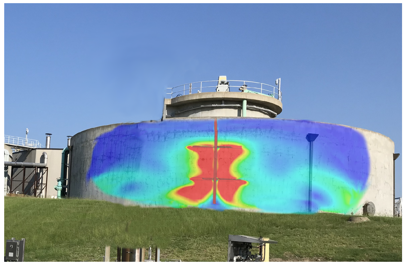
Modelling the mass transport and hydrodynamic behaviour of fluids and particles in anaerobic digestion has been an emerging research field in recent years. Computational Fluid Dynamics (CFD) is an established modelling tool that uses the mathematics of fluid mechanics (e.g., Navier–Stokes, Euler equations) and numerical analysis to solve the governing equations on a 1- to 3-dimensional discretised grid [166]. As computational capabilities have increased (see Section 1), so the possibilities for using CFD to influence design and performance of AD reactors, especially related to mixing efficiency and identification of flow issues, have become a viable tool for multi-disciplinary research teams [167] and modelling consultancies (see Figure 4 for an example of CFD employed at full-scale). This is reflected by the increasing number of studies and software platforms that use CFD for AD research, including the performance of gas-mixing [168], physical mixing [169,170], process design and optimisation [171].
The use of CFD in anaerobic digestion processes, whether for reactor mixing and design or process optimisation, is likely to become a valuable tool for process engineers. At present it is used as a complementary approach with models that describe biochemical reactions through dynamic integration. However, recent studies have looked at using CFD models with biological kinetics and advection-diffusion transport of soluble metabolites and biomass, in a similar way to the methods for modelling spatially realised biofilm growth [172,173].
5.4. Individual-Based Modelling
We have seen that modelling of anaerobic digestion, and bioprocesses more broadly, have evolved and diversified as knowledge has accrued at different scales and computational capacity has dramatically increased. Although mechanistic models are likely to persist as the method of choice for engineers and practitioners, other approaches will emerge that offer those working in AD with tools to enhance their understanding and management of these systems. One such method that is highly granular and explicitly resolved is individual-based modelling. Individual-based Models (IbMs) and associated tools, such as agent-based models and cellular automata (CA), are spatio-dynamical and discrete in time, space and states. Although CA are typically used to predict geometric distributions based on local interactions, IbMs are highly resolved at the cell or individual level [79,174]. Unlike aggregated and continuous population models, IbMs proscribe behavioural physical and biological traits to individuals in a highly discretised manner, where the complex, global behaviour of the population emerges from the simpler, local properties and interactions among individuals.
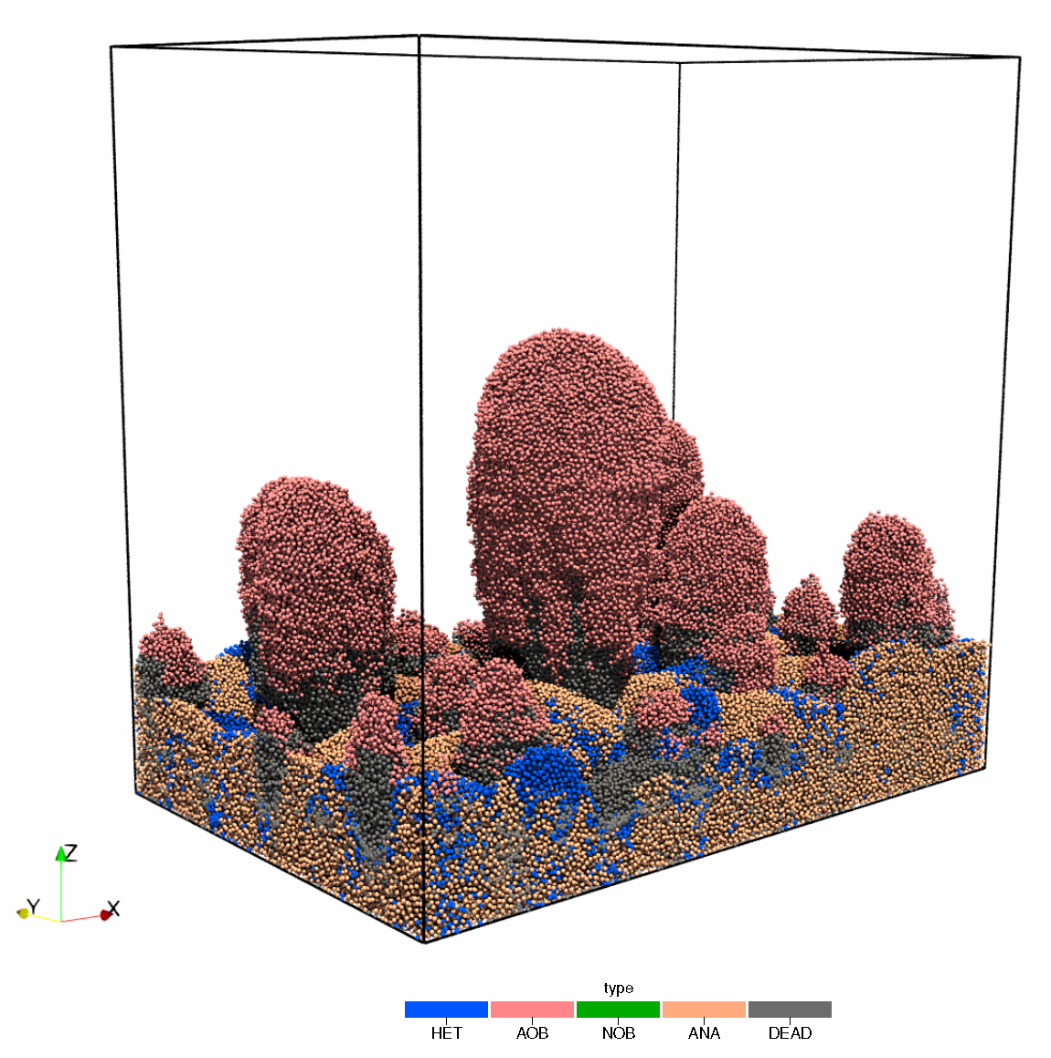
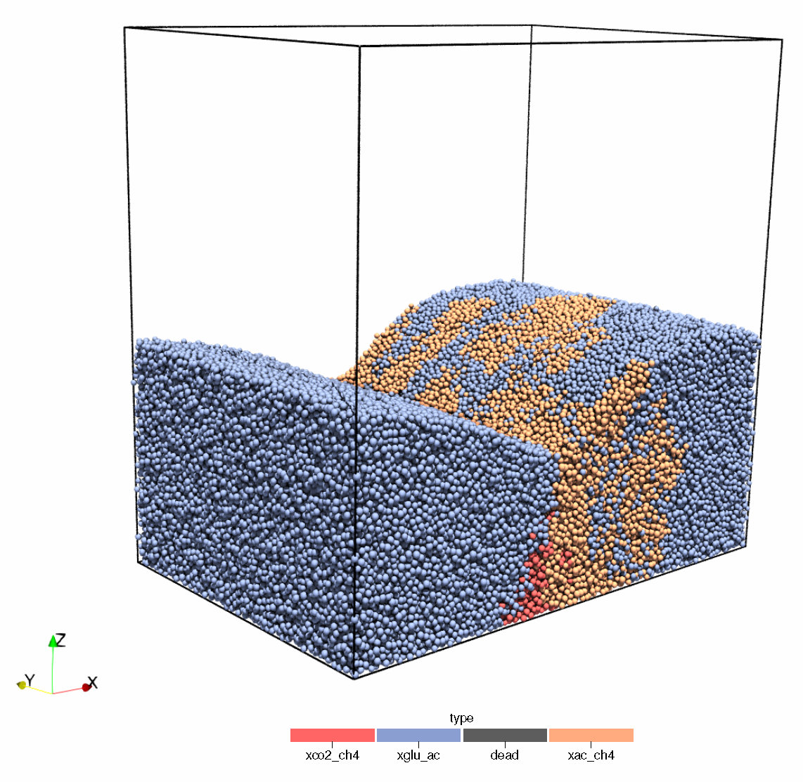
IbMs have historically been used in macro-ecology but found significant purchase as a tool for modelling biofilms, building on knowledge gained from spatio-temporal, multi-species biomass-based models, such as those briefly mentioned in Section 3 [175,176]. In addition to the microbial growth properties, physical interactions between individuals, motility, environmental gradients, fluid dynamics, thermodynamics, and even stochasticity may also be included as hybrid components to a more comprehensive process, sub-process or reactor scale model [177,178,179]. Such a multi-scale model is complex and requires a large degree of multi-disciplinarity to ensure successful implementation. However, the use of IbMs is becoming more ubiquitous and recent efforts to develop large-scale simulators of EBS using hybrid IbM and statistical emulators have established a framework for studying microbial community behaviour at scale [71,180,181], opening the door for application to anaerobic digestion processes [179,182] (See Figure 5 for an example application of an IbM applied to anaerobic processes).
6. Conclusions
With five decades of anaerobic digestion mathematical modelling there may be an assumption of consensus among the scientific and engineering communities who have directly or indirectly aided the development and validation of models from theory to practice. Although it could be argued that there is a level of maturity embodied by the most well-known and used tool, the Anaerobic Digestion Model No. 1, we have seen that such highly structured, complex models do not fit all purposes. Indeed, many applications of empirically derived mechanistic models rely on simplifying assumptions to obtain a structure that is identifiable, without loss of specificity or accuracy, e.g., for process control. Here we argue that the rigorous application of mathematical analysis tools, typically in the domain of theorists, can be appropriately applied to reduced-order models of AD to investigate the qualitative behaviour of the system, identifying unexpected behaviour, guiding experimental studies, and suggesting suitable control parameter limits for improved process operation.
Many of the bottlenecks that have limited not only modelling but more general AD research, such as reliable and in situ instrumentation, limited understanding of the complex microbial ecology of digesters, and restrictive computational capacity, have generally been overcome in the last two decades. This has manifested, more widely, in the large availability of data in the bioprocess industry, opening up opportunities for AD modelling across scales, from the cellular and metabolic level, through to plant-wide integration and supervisory control. Although data-driven models and digital tools based on machine learning algorithms and AI are emerging in parallel with the Industry 4.0 ethos of “Smart Systems”, it is cautioned by the well-known aphorism “garbage in, garbage out”. There are a significant number of publications on the use of AI techniques such as Artificial Neural Networks, but these may be subject to the problem of over-fitting and loss of generality. Investment in time and energy to develop complexity is driven by an assumption that the more information the better the model. This is not strictly true, many soft-sensors employed today are based on simple multivariate relationships between a few measured variables, where a standard PLS regression model may be adequate.
However, to address more challenging issues faced by industry, it is clear that some standard modelling approaches may not be fit for purpose. The future of AD modelling will track the needs of the industry but also incorporate ideas from other fields to ensure that models are robust, reliable, flexible and adaptable to local and global shifts in the process domain. We are already seeing this happen in the water sector, where environmental challenges such as climate change, increased urbanisation and economic constraints, are driving industries to look at the potential for models to ensure that infrastructure is resilient in the face of novel demands. AD technology is a key component of the energy-food-water nexus and drivers already exist for collaboration between modelers, engineers, scientists and other stakeholders to exploit the potential of available models but also to integrate emerging and innovative methods into their thinking around AD, such as hybrid modelling techniques, cellular level and metabolic knowledge, thermodynamic constraints on microbial growth, fluid dynamic process visualisation, and fine-grain individual scale models that can incorporate all of these elements.
This review does not suggest a preference for any model or modelling approach. There is no ideal model for AD and often several models may achieve the same goal. Simply, we present a broad overview of the historical context of AD modelling and look to the future as the wealth of knowledge and information grows. The use of models for AD is strengthening and we envisage that this will become even more important in the context of the climate emergency, the need for smart management of resources and in the provision of resilient infrastructure that generate and process these resources.
Funding
This work was funded by the European Union’s Horizon 2020 Research and Innovation Programme under the Marie Skłodowska-Curie Grant Agreement No. 702408 (DRAMATIC).
Acknowledgments
The author wishes to thank Wim Audenaert (AM-Team, Ghent) and Bowen Li (Newcastle University) for permission to use the images acknowledged in the manuscript. The author thanks Tewfik Sari (INRAE, Montpellier) and the anonymous reviewers for their insightful and helpful comments on the manuscript.
Conflicts of Interest
The author declares no conflict of interest.
Abbreviations
The following abbreviations are used in this manuscript:
| AD | Anaerobic Digestion |
| ADM1 | Anaerobic Digestion Model No. 1 |
| AI | Artificial Intelligence |
| ANN | Artificial Neural Network |
| ASMx | Activated Sludge Model No. (x) |
| BOD | Biochemical Oxygen Demand |
| CA | Cellular Automata |
| CFD | Computational Fluid Dynamics |
| COD | Chemical Oxygen Demand |
| DAE | Differential Algebraic Equations |
| EBS | Engineered Biological Systems |
| FBA | Flux Balance Analysis |
| IbM | Individual-based Model |
| ODE | Ordinary Differential Equation |
| OPLS | Ordinary Partial Least Squares |
| PCA | Principal Component Analysis |
| PDE | Partial Differential Equation |
| PLS | Partial Least Squares |
| VFA | Volatile Fatty Acids |
| VSS | Volatile Suspended Solids |
Appendix A. Bifurcation Analysis Example
Assuming no biomass enters the reactor, Equations (2) and (3) can be rewritten (after switching the order) as
where D is the dilution rate, is the influent substrate concentration, and is the non-monotonic Haldane growth function of the organism growing on . To determine the equilibria of the system, we now set the LHS of the equations to zero and solve the equalities for and . This results in the identification of three possible steady states defined analytically by
where and are the steady-state concentrations of and , respectively (See Appendix A for details).
To calculate the stability of the equilibria, we first construct the Jacobian matrix of the system
For each equilibrium, we can substitute expressions for and at steady-state into the Jacobian and check its eigenvalues, knowing that , where I is the identity matrix and s are the eigenvalues that satisfy the equation. Taking, for example, the washout equilibria , the eigenvalues are determined analytically to be [, ]. Hence, we can now derive an explicit condition that states is meaningful and stable () for . In biological terms, this means if the dilution rate is higher than the growth rate of the organism, its washout is guaranteed, a common observation that links chemostat theory with empirical understanding. We can also find analytical expressions for the existence, uniqueness and stability of the other two equilibria but omit them here for brevity. Layperson definitions: Existence: Conditions for which an equilibrium exists; Uniqueness: Under the conditions for existence, is the criteria for one and only one equilibrium satisfied? Stability: Given some arbitrarily small perturbation away from the equilibrium, does the system return to that equilibrium (local stability)? Does the system return to an equilibrium from any permissible point in that system (global stability)? The Routh-Hurwitz criterion and Lyupanov functions are common methods used to test stability for systems of ODEs [184].
Unless these analytical expressions are transparent to interpretation, it is often difficult to extract practical knowledge from them. However, because they describe the general and immutable behaviour of the system, local bifurcation analysis can be used as a complementary method for visual interpretation of existence and stability of equilibria. For engineering purposes, bifurcation analysis is usually performed using free system parameters, i.e., the operating or control parameters that can be adjusted. However, bifurcation using fixed or unidentifiable parameters can provide useful knowledge for model fitting when there is a degree of parameter uncertainty, or potentially where microbial traits can be adapted or evolved (e.g., synthetic biology, bioengineering, bioaugmentation).
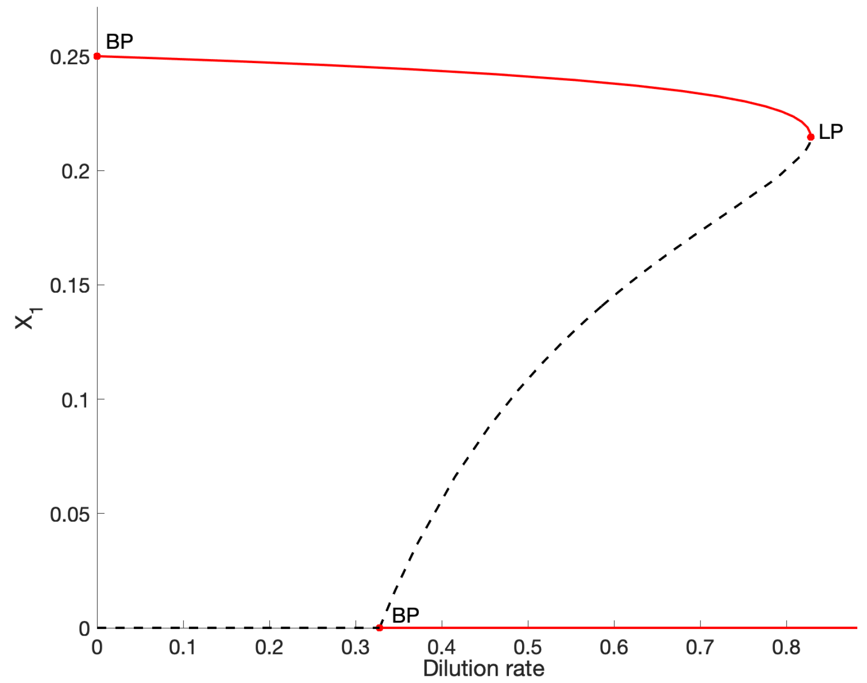
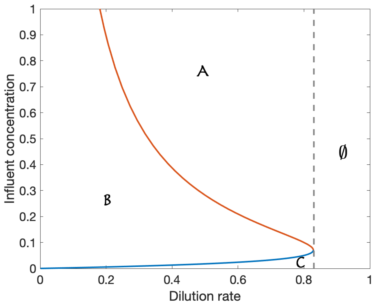
We conduct a numerical analysis of the model by assigning parameter values, shown in Table A1, to the model. A one-parameter bifurcation, using dilution rate as the bifurcating parameter, is shown in Figure A1. Briefly, the analysis identifies stable (red) and unstable (dashed black) equilibria in the variable domain. Two branch points (BP) representing the switching between two equilibria, and a limit point (LP) where two equilibria collide (or emerge), are identified. Biological interpretation: LP represents the maximum dilution rate at which a positive concentration is possible. A two-parameter bifurcation diagram is shown in Figure A2. This is sometimes referred to as an operating diagram as it allows for the identification of stable operating regions. In this case, maintaining a dilution rate below 0.8284 and an acetate influent concentration between the blue and red curves guarantees stable existence of the acetate degrader. Increasing this concentration, so that the process is operating above the red curve in a region of bistability, would require control of the initial conditions to avoid the washout case.

Table A1.
Parameter set for bifurcation analysis example.
| Parameter | Value |
|---|---|
| 2.0 | |
| Y | 0.5 |
| 0.05 | |
| 0.1 | |
| 0.5 | |
| D | 0.4 |
Figure A1.
One-parameter bifurcation in for the parameter set given in Table A1 indicating a limit point (saddle-node bifurcation), LP, at a dilution rate of 0.8284 at the collision of two equilibria ( and ). The red line corresponds to stable fixed points (equilibria) and dashed black line to unstable fixed points. It can be noted that at D > 0.3279, the system is bistable in and . The branch point (BP) at D = 0, corresponds to the theoretical maximum , where no biomass or substrate leaves the reactor.

Figure A2.
Two-parameter bifurcation diagram: A Bistable Unstable , B Stable Unstable , C Stable , Unstable , ∅ Stable .
Figure A2.
Two-parameter bifurcation diagram: A Bistable Unstable , B Stable Unstable , C Stable , Unstable , ∅ Stable .

References
- Makinia, J. Mathematical Modelling and Computer Simulation of Activated Sludge Systems; IWA Publishing: London, UK, 2010. [Google Scholar]
- van Loosdrecht, M.C.M.; Lopez-Vazquez, C.M.; Meijer, S.C.F.; Hooijmans, C.M.; Brdjanovic, D. Twenty-five years of ASM1: Past, present and future of wastewater treatment modelling. J. Hydroinform. 2015, 17, 697–718. [Google Scholar] [CrossRef] [Green Version]
- Henze, M.; Grady, J.R.C.P.; Gujer, W.; Marais, G.; Matsuo, T. Activated Sludge Model No 1; IAWPRC Scientific and Technical Report No. 1; IAWQ: London, UK, 1987. [Google Scholar]
- Henze, M.; Gujer, W.; Mino, T.; Matsuo, T.; Wentzel, M.C.; Marais, G.v.R. Activated Sludge Model No. 2; IAWQ Scientific and Technical Report No. 3; IAWQ: London, UK, 1995. [Google Scholar]
- Henze, M.; Gujer, W.; Mino, T.; Matsuo, T.; Wentzel, M.C.; Marais, G.v.R.; van Loosdrecht, M.C.M. Activated Sludge Model No. 2d, ASM2d. Water Sci. Technol. 1999, 39, 165–182. [Google Scholar] [CrossRef]
- Batstone, D.J.; Keller, J.; Angelidaki, I.; Kalyuzhnyi, S.V.; Pavlostathis, S.G.; Rozzi, A.; Sanders, W.T.M.; Siegrist, H.; Vavilin, V.A. Anaerobic Digestion Model No. 1; Technical Report Report No. 13; IWA Publishing: London, UK, 2002. [Google Scholar]
- Jeppsson, U.; Rosen, C.; Alex, J.; Copp, J.B.; Gernaey, K.V.; Pons, M.N.; Vanrolleghem, P.A. Towards a benchmark simulation model for plant-wide control strategy performance evaluation of WWTPs. Water Sci. Technol. 2006, 53, 287–295. [Google Scholar] [CrossRef] [PubMed]
- Jeppsson, U.; Pons, M.N.; Nopens, I.; Alex, J.; Copp, J.B.; Gernaey, K.V.; Rosen, C.; Steyer, J.P.; Vanrolleghem, P.A. Benchmark Simulation Model No. 2—General protocol and exploratory case studies. Water Sci. Technol. 2007, 56, 67–78. [Google Scholar] [CrossRef] [PubMed]
- Rosen, C.; Vrecko, D.; Gernaey, K.; Pons, M.; Jeppsson, U. Implementing ADM1 for plant-wide benchmark simulations in Matlab/Simulink. Water Sci. Technol. 2006, 54, 11–19. [Google Scholar] [CrossRef]
- Arnell, M.; Rahmberg, M.; Oliveira, F.; Jeppsson, U. Multi-objective performance assessment of wastewater treatment plants combining plant-wide process models and life cycle assessment. J. Water Clim. Chang. 2017, 8, 715–729. [Google Scholar] [CrossRef]
- Fernández-Arévalo, T.; Lizarralde, I.; Fdz-Polanco, F.; Pérez-Elvira, S.I.; Garrido, J.M.; Puig, S.; Poch, M.; Grau, P.; Ayesa, E. Quantitative assessment of energy and resource recovery in wastewater treatment plants based on plant-wide simulations. Water Res. 2017, 118, 272–288. [Google Scholar] [CrossRef]
- Solon, K.; Mingsheng, J.; Volcke, E.I.P. Process schemes for future energy-positive water resource recovery facilities. Water Sci. Technol. 2019, 79, 1808–1820. [Google Scholar] [CrossRef]
- Maere, T.; Verrecht, B.; Moerenhout, S.; Judd, S.; Nopens, I. BSM-MBR: A benchmark simulation model to compare control and operational strategies for membrane bioreactors. Water Res. 2011, 45, 2181–2190. [Google Scholar] [CrossRef] [Green Version]
- Seco, A.; Ruano, M.V.; Ruiz-Martinez, A.; Robles, A.; Barat, R.; Serralta, J.; Ferrer, J. Plant-wide modelling in wastewater treatment: Showcasing experiences using the Biological Nutrient Removal Model. Water Sci. Technol. 2020, 81, 1700–1714. [Google Scholar] [CrossRef]
- Fedorovich, V.; Lens, P.; Kalyuzhnyi, S. Extension of Anaerobic Digestion Model No. 1 with processes of sulfate reduction. Appl. Biochem. Biotechnol. 2003, 109, 33–45. [Google Scholar] [CrossRef]
- Batstone, D.J.; Keller, J.; Steyer, J.P. A review of ADM1 extensions, applications, and analysis: 2002–2005. Water Sci. Technol. 2006, 54, 1–10. [Google Scholar] [CrossRef] [PubMed]
- Flores-Alsina, X.; Solon, K.; Mbamba, C.K.; Tait, S.; Gernaey, K.V.; Jeppsson, U.; J.Batstone, D. Modelling phosphorus (P), sulfur (S) and iron (Fe) interactions for dynamic simulations of anaerobic digestion processes. Water Res. 2016, 95, 370–382. [Google Scholar] [CrossRef] [PubMed] [Green Version]
- Frunzo, L.; Fermoso, F.G.; Luongo, V.; Mattei, M.R.; Esposito, G. ADM1-based mechanistic model for the role of trace elements in anaerobic digestion processes. J. Environ. Manag. 2019, 241, 587–602. [Google Scholar] [CrossRef]
- Siegrist, H.; Vogt, D.; Garcia-Heras, J.; Gujer, W. Mathematical model for meso and thermophilic anaerobic sewage sludge digestion. Environ. Sci. Technol. 2002, 36, 1113–1123. [Google Scholar] [CrossRef]
- Elmitwalli, T.A.; Sayed, S.; Groendijk, L.; van Lier, J.; Zeeman, G.; Lettinga, G. Decentralised treatment of concentrated sewage at low temperature in a two-step anaerobic system: Two upflow-hybrid septic tanks. Water Sci. Technol. 2003, 48, 219–226. [Google Scholar] [CrossRef]
- Copp, J.; Peerbolte, A.; Snowling, S.; Schraa, O.; Froelich, D.; Belia, E. Integrating anaerobic digestion into plant-wide wastewater treatment modelling—Experience with data from a large treatment plant. In Proceedings of the Anaerobic Digestion 2004, 10th World Congress on Anaerobic Digestion, Montréal, QC, Canada, 29 August–2 September 2004; pp. 1362–1365. [Google Scholar]
- Batstone, D.J.; Puyol, D.; Flores-Alsina, X.; Rodríguez, J. Mathematical modelling of anaerobic digestion processes: Applications and future needs. Rev. Environ. Sci. Biotechnol. 2015, 14, 595–613. [Google Scholar] [CrossRef]
- Arzate, J.A.; Kirstein, M.; Ertem, F.C.; Kielhorn, E.; Ramirez Malule, H.; Neubauer, P.; Cruz-Bournazou, M.N.; Junne, S. Anaerobic Digestion Model (AM2) for the Description of Biogas Processes at Dynamic Feedstock Loading Rates. Chem. Ing. Tech. 2017, 89, 686–695. [Google Scholar] [CrossRef]
- Hoffmann, D.S. The dawn of mathematical biology. arXiv 2015, arXiv:physics.hist-ph/1511.01455. [Google Scholar]
- Michaelis, L.; Menten, M.L. Die Kinetik der Invertinwirkung [The kinetics of invertase activity]. Biochem. Z. 1913, 49, 333–369. [Google Scholar]
- Israel, G. On the Contribution of Volterra and Lotka to the Development of Modern Biomathematics. Hist. Philos. Life Sci. 1988, 10, 37–49. [Google Scholar] [PubMed]
- Monod, J. Recherches sur la Croissance des Cellules Bactériennes [Research on the Growth of Bacterial Cells]. Ph.D. Thesis, Université de Paris, Paris, France, 1941. [Google Scholar]
- Wade, M.J.; Harmand, J.; Benyahia, B.; Bouchez, T.; Chaillou, S.; Cloez, B.; Godon, J.; Moussa Boudjemaa, B.; Rapaport, A.; Sari, T.; et al. Perspectives in mathematical modelling for microbial ecology. Ecol. Modell. 2016, 321, 64–74. [Google Scholar] [CrossRef]
- Andrews, J.F. A Mathematical Model for the Continuous Culture of Microorganisms Utilizing Inhibitory Substrate. Biotechnol. Bioeng. 1968, 10, 707–723. [Google Scholar] [CrossRef]
- Andrews, J.F. Dynamic model of the anaerobic digestion process. J. Sanit. Eng. Div. Am. Soc. Civ. Eng. 1969, 95, 95–116. [Google Scholar]
- Lawrence, A.W.; McCarty, P.L. Kinetics of methane fermentation in anaerobic treatment. J. Water Pollut. Control Fed. 2009, 41, R1–R17. [Google Scholar]
- Lawrence, A.W. Application of Process Kinetics to Design of Anaerobic Processes. In Anaerobic Biological Treatment Processes; American Chemical Society: Washington, DC, USA, 1971; Volume 105, pp. 163–190. [Google Scholar] [CrossRef]
- Andrews, J.F.; Graef, S.P. Dynamic modelling and Simulation of the Anaerobic Digestion Process. In Anaerobic Biological Treatment Processes; American Chemical Society: Washington, DC, USA, 1971; Volume 105, pp. 126–162. [Google Scholar] [CrossRef]
- Barnett, M.W.; Stenstrom, M.K.; Andrews, J.F. Dynamics and Control of Wastewater Systems, 2nd ed.; CRC Press, Inc.: Lancaster, PA, USA, 1998; Volume 6. [Google Scholar]
- Andrews, J.F. Dynamic models and control strategies for wastewater treatment processes. Water Res. 1974, 8, 261–289. [Google Scholar] [CrossRef]
- Graef, S.P.; Andrews, J.F. Stability and control of anaerobic digestion. J. Water Pollut. Control Fed. 1974, 46, 666–683. [Google Scholar]
- Collins, A.S.; Guilliland, B.E. Control of anaerobic digestion process. J. Environ. Eng. Div. 1974, 2, 487–506. [Google Scholar] [CrossRef]
- Simeonov, I.; Momchev, V.; Grancharov, D. Dynamic modelling of mesophilic anaerobic digestion of animal waste. Water Res. 1996, 30, 1087–1094. [Google Scholar] [CrossRef]
- Andrews, J.F. Development of Control Strategies for Waste-Water Treatment Plants. In Instrumentation Control and Automation for Waste-Water Treatment Systems; Andrews, J., Briggs, R., Jenkins, S., Eds.; Pergamon: New York, NY, USA, 1974; pp. 233–243. [Google Scholar] [CrossRef]
- Olsson, G.; Nielsen, M.; Yuan, Z.; Lynggaard-Jensen, A.; Steyer, J.P. Instrumentation, Control and Automation in Wastewater Systems; IWA Publishing: London, UK, 2005. [Google Scholar] [CrossRef]
- Hill, D.T.; Barth, C.L. A dynamic model for simulation of animal waste digestion. J. Wat. Pollut. Control Fed. 1977, 10, 2129–2143. [Google Scholar]
- Lyberatos, G.; Skiadas, I.V. Modelling of Anaerobic Digestion—A Review. Glob. Nest Int. J. 1999, 1, 63–76. [Google Scholar] [CrossRef]
- Ficara, E.; Hassam, S.; Allegrini, A.; Leva, A.; Malpei, F.; Ferretti, G. Anaerobic Digestion Models: A Comparative Study. IFAC Proc. Vol. 2012, 45, 1052–1057. [Google Scholar] [CrossRef]
- Kythreotou, N.; Florides, G.; Tassou, S.A. A review of simple to scientific models for anaerobic digestion. Renew. Energy 2014, 71, 701–714. [Google Scholar] [CrossRef]
- Hill, D.T. A comprehensive dynamic model for animal waste methanogenesis. Trans. ASAE 1982, 25, 1374–1380. [Google Scholar] [CrossRef]
- Hill, D.T. Design parameters and operating characteristics of animal waste anaerobic digestion systems—Swine and poultry. Agric. Wastes 1983, 5, 157–178. [Google Scholar] [CrossRef]
- Mosey, F.E. Mathematical Modelling of the Anaerobic Digestion Process: Regulatory Mechanisms for the Formation of Short-Chain Volatile Acids from Glucose. Water Sci. Technol. 1983, 15, 209–232. [Google Scholar] [CrossRef]
- Bryers, J.D. Structured modelling of the anaerobic digestion of biomass particulates. Biotechnol. Bioeng. 1984, 27, 638–649. [Google Scholar] [CrossRef]
- Pavlostathis, S.G.; Gossett, J.M. A kinetic model for anaerobic digestion of biological sludge. Biotech. Bioeng. 1986, 28, 1519–1530. [Google Scholar] [CrossRef]
- Moletta, R.; Verrier, D.; Albagnac, G. Dynamic modelling of anaerobic digestion. Water Res. 1986, 20, 427–434. [Google Scholar] [CrossRef]
- Angelidaki, I.; Ellegaard, L.; Ahring, B. A mathematical model for dynamic simulation of anaerobic digestion of complex substrates: Focusing on ammonia inhibition. Biotechnol. Bioeng. 1993, 42, 159–166. [Google Scholar] [CrossRef]
- Siegrist, H.; Renggli, D.; Gujer, W. Mathematical modelling of anaerobic mesophilic sewage sludge treatment. Water Sci. Technol. 1993, 27, 25–36. [Google Scholar] [CrossRef]
- Vavilin, V.A.; Vasiliev, V.B.; Ponomarev, A.V.; Rytow, S.V. Simulation model ‘methane’ as a tool for effective biogas production during anaerobic conversion of complex organic matter. Bioresour. Technol. 1994, 48, 1–8. [Google Scholar] [CrossRef]
- Chen, Y.R.; Hashimoto, A.G. Substrate utilization kinetic model for biological treatment process. Biotechnol. Bioeng. 1980, 22, 2081–2095. [Google Scholar] [CrossRef] [PubMed]
- Gujer, W.; Zehnder, A.J.B. Conversion processes in anaerobic digestion. Water Sci. Technol. 1983, 15, 127–167. [Google Scholar] [CrossRef]
- Dolfing, J. Kinetics of methane formation by granular sludge at low substrate concentrations. Appl. Microbiol. Biotech. 1985, 22, 77–81. [Google Scholar] [CrossRef]
- Gavala, H.N.; Angelidaki, I.; Ahring, B.K. Kinetics and modelling of Anaerobic Digestion Process. In Biomethanation I. Advances in Biochemical Engineering/Biotechnology; Ahring, B.K., Ed.; Springer: Berlin/Heidelberg, Germany, 2003; Volume 81, pp. 126–162. [Google Scholar] [CrossRef]
- Kaspar, H.F. Untersuchungen zur Kopplung von Wasserstoff- und Methanbildung im Faulschlamm [Studies on the Coupling of Hydrogen and Methane Formation in Digested Sludge]. Ph.D. Thesis, Swiss Federal Institute of Technology, Zürich, Switzerland, 1977. [Google Scholar] [CrossRef]
- Irvine, R.L.; Alleman, J.E.; Miller, G.; Dennis, R.W. Stoichiometry and Kinetics of Biological Waste Treatment. J. Water Pollut. Control Fed. 1980, 52, 1997–2006. [Google Scholar] [CrossRef]
- Kleerebezem, R.; van Loosdrecht, M.C.M. Critical analysis of some concepts proposed in ADM1. Water Sci. Technol. 2006, 54, 51–57. [Google Scholar] [CrossRef]
- Petersen, E.E. Chemical Reaction Analysis; Prentice-Hall: Englegood Cliffs, NJ, USA, 1965. [Google Scholar]
- Christ, O.; Wilderer, P.A.; Angerhöfer, R.; Faulstich, M. Mathematical modelling of the hydrolysis of anaerobic processes. Water Sci. Technol. 2000, 41, 61–65. [Google Scholar] [CrossRef]
- Jeyaseelan, S. A simple mathematical model for anaerobic digestion process. Water Sci. Technol. 1997, 35, 185–191. [Google Scholar] [CrossRef]
- Angelidaki, I.; Ellegaard, L.; Ahring, B. A comprehensive model of anaerobic bioconversion of complex substrates to biogas. Biotechnol. Bioeng. 1999, 63, 363–372. [Google Scholar] [CrossRef]
- Blumensaat, F.; Keller, J. Modelling of two-stage anaerobic digestion using the IWA Anaerobic Digestion Model No. 1 (ADM1). Water Res. 2005, 39, 171–183. [Google Scholar] [CrossRef] [PubMed]
- Galí, A.; Benabdallah, T.; Astals, S.; Mata-Alvarez, J. Modified version of ADM1 model for agro-waste application. Bioresour. Technol. 2009, 100, 2783–2790. [Google Scholar] [CrossRef]
- Gaida, D.; Wolf, C.; Meyer, C.; Stuhlsatz, A.; Uppel, J.; Back, T.; Bongards, M.; McLoone, S. State estimation for anaerobic digesters using the ADM1. Water Sci. Technol. 2012, 66, 1088–1094. [Google Scholar] [CrossRef] [PubMed]
- Liotta, F.; Chatellier, P.; Esposito, G.; Fabbricino, M.; Frunzo, L.; van Hullebusch, E.D.; Lens, P.N.L.; Pirozzi, F. Modified Anaerobic Digestion Model No.1 for dry and semi-dry anaerobic digestion of solid organic waste. Environ. Technol. 2015, 36, 870–880. [Google Scholar] [CrossRef] [PubMed] [Green Version]
- Zhao, X.; Li, L.; Wu, D.; Xiao, T.; Ma, Y.; Peng, X. Modified Anaerobic Digestion Model No. 1 for modelling methane production from food waste in batch and semi-continuous anaerobic digestions. Bioresour. Technol. 2019, 271, 109–117. [Google Scholar] [CrossRef] [PubMed]
- Batstone, D.J.; Keller, J. Industrial applications of the IWA anaerobic digestion model No. 1 (ADM1). Water Sci. Technol. 2003, 47, 199–206. [Google Scholar] [CrossRef] [PubMed] [Green Version]
- Li, X.; Yang, Z.; Liu, G.; Ma, Z.; Wang, W. Modified anaerobic digestion model No.1 (ADM 1) for modelling anaerobic digestion process at different ammonium concentrations. Water Environ. Res. 2019, 91, 700–714. [Google Scholar] [CrossRef]
- Lauwers, J.; Nimmegeers, P.; Logist, F.; Van Impe, J. Structural identifiability analysis of the Anaerobic Digestion Model No. 1 using a local algebraic observability approach. IFAC-PapersOnLine 2015, 48, 470–475. [Google Scholar] [CrossRef]
- Bernard, O.; Hadj-Sadok, Z.; Dochain, D.; Genovesi, A.; Steyer, J. Dynamical model development and parameter identification for an anaerobic wastewater treatment process. Biotechnol. Bioeng. 2001, 75, 424–438. [Google Scholar] [CrossRef]
- Sbarciog, M.; Loccufier, M.; Noldus, E. Determination of appropriate operating strategies for anaerobic digestion systems. J. Math. Biosci. 2010, 51, 180–188. [Google Scholar] [CrossRef]
- Benyahia, B.; Sari, T.; Cherki, B.; Harmand, J. Bifurcation and stability analysis of a two step model for monitoring anaerobic digestion processes. J. Proc. Control 2012, 22, 1008–1019. [Google Scholar] [CrossRef] [Green Version]
- Sari, T.; Benyahia, B. The operating diagram for a two-step anaerobic digestion model. arXiv 2020, arXiv:math.DS/2004.14028. [Google Scholar]
- Donoso-Bravo, A.; Mailier, J.; Martin, C.; Rodríguez, J.; Arturo Aceves-Lara, C.; Van de Wouwer, A. Model selection, identification and validation in anaerobic digestion: A review. Water Res. 2011, 45, 5347–5364. [Google Scholar] [CrossRef] [PubMed]
- Oreskes, N.; Belitz, K. Philosophical issues in model assessment. In Model Validation: Perspectives in Hydrological Science; Anderson, M.G., Bates, P.D., Eds.; Wiley: Chichester, UK, 2001; pp. 23–41. [Google Scholar]
- Song, H.; Cannon, W.R.; Beliaev, A.S.; Konopka, A. Mathematical modelling of Microbial Community Dynamics: A Methodological Review. Processes 2014, 2, 711–752. [Google Scholar] [CrossRef] [Green Version]
- Laureni, M.; Weissbrodt, D.G.; Villez, K.; Robin, O.; de Jonge, N.; Rosenthal, A.; Wells, G.; Lund Nielsen, J.; Morgenroth, E.; Joss, A. Biomass segregation between biofilm and flocs improves the control of nitrite-oxidizing bacteria in mainstream partial nitritation and anammox processes. Water Res. 2019, 154, 114–116. [Google Scholar] [CrossRef]
- Eberl, H.; Wade, M.J. Challenges and perspectives in reactor scale modelling of biofilm processes. In Recent Trends in Biofilm Science and Technology; Simoes, M., Borges, A., Chaves Simoes, L., Eds.; Academic Press: Cambridge, MA, USA, 2020; pp. 81–120. [Google Scholar]
- Bernard, O.; Chachuat, B.; Héllias, A.; Rodriguez, J. Can we assess the model complexity for a bioprocess: Theory and example of the anaerobic digestion process. Water Sci. Technol. 2006, 53, 175–182. [Google Scholar] [CrossRef]
- Azeiteiro, C.; Capela, I.F.; Durate, A.C. Dynamic model simulations as a tool for evaluating the stability of an anaerobic process. Water SA 2001, 27, 109–114. [Google Scholar] [CrossRef] [Green Version]
- Steyer, J.P.; Buffiere, P.; Rolland, D.; Moletta, R. Advanced control of anaerobic digestion process through disturbances monitoring. Water Res. 1999, 33, 2059–2068. [Google Scholar] [CrossRef]
- Marsili-Libelli, S.; Nardini, M. Stability and sensitivity analysis of anaerobic digestion models. Environ. Technol. Lett. 1985, 6, 602–609. [Google Scholar] [CrossRef]
- Marsili-Libelli, S.; Beni, S. Shock load modelling in the anaerobic digestion process. Ecol. Modell. 1996, 84, 215–232. [Google Scholar] [CrossRef]
- Brodland, G.W. How computational models can help unlock biological systems. Semin. Cell Dev. Biol. 2015, 47–48, 62–73. [Google Scholar] [CrossRef] [Green Version]
- Suh, N.P. On functional periodicity as the basis for long-term stability of engineered and natural systems and its relationship to physical laws. Res. Eng. Des. 2004, 15, 72–75. [Google Scholar] [CrossRef]
- Bernard, O.; Polit, M.; Hadj-Sadok, Z.; Pengov, M.; Dochain, D.; Estaben, M.; Labat, P. Advanced monitoring and control of anaerobic wastewater treatment plants: Software sensors and controllers for an anaerobic digester. Water Sci. Technol. 2001, 43, 175–182. [Google Scholar] [CrossRef] [PubMed]
- Rincón, A.; Angulo, F.O.G. Control of an anaerobic digester through normal form of fold bifurcation. J. Proc. Cont. 2009, 19, 1355–1367. [Google Scholar] [CrossRef]
- Dimitrova, N.; Krastanov, M. Model-based control strategies for anaerobic digestion processes. Biomath 2019, 8, 1907127. [Google Scholar] [CrossRef] [Green Version]
- Hess, J.; Bernard, O. Design and study of a risk management criterion for an unstable wastewater treatment process. J. Process Control 2008, 18, 71–79. [Google Scholar] [CrossRef]
- Abdelkader, O.H.; Abdelkader, A.H. Modelling Anaerobic Digestion Using Stochastic Approaches. In Trends in Biomathematics: Mathematical modelling for Health, Harvesting, and Population Dynamics: Selected Works Presented at the BIOMAT Consortium Lectures, Morocco 2018; Springer International Publishing: Cham, Switzerland, 2019; pp. 373–396. [Google Scholar] [CrossRef]
- Bailey, J.E. Mathematical modelling and analysis in biochemical engineering: Past accomplishments and future opportunities. Biotechnol. Progress 1998, 14, 8–20. [Google Scholar] [CrossRef]
- Powell, G. Stable coexistence of syntrophic associations in continuous culture. J. Chem. Technol. Biotechnol. 1985, 35, 46–50. [Google Scholar] [CrossRef]
- Hajji, M.; Mazenc, F.; Harmand, J. A mathematical study of syntrophic relationship of a model of anaerobic digestion process. Biosci. Eng. 2010, 7, 641–656. [Google Scholar] [CrossRef]
- Volcke, E.I.P.; Sbarciog, M.; Noldus, E.J.L.; De Baets, B.; Loccufier, M. Steady state multiplicity of two-step biological conversion systems with general kinetics. Math. Biosci. 2010, 228, 160–170. [Google Scholar] [CrossRef] [Green Version]
- Volcke, E.I.P.; Loccufier, M.; Vanrolleghem, P.A.; Noldus, E.J.L. Existence, uniqueness and stability of the equilibrium points of a SHARON bioreactor model. J. Proc. Cont. 2006, 16, 1003–1012. [Google Scholar] [CrossRef]
- Wade, M.J.; Wolkowicz, G.S.K. Bifurcation analysis of an impulsive system describing a Partial Nitritation and Anammox in a hybrid reactor. bioRxiv 2020. [Google Scholar] [CrossRef] [Green Version]
- Wade, M.J.; Pattinson, R.W.; Parker, N.G.; Dolfing, J. Emergent behaviour in a chlorophenol-mineralising three-tiered microbial ‘food web’. J. Theor. Biol. 2016, 389, 171–186. [Google Scholar] [CrossRef] [PubMed] [Green Version]
- Sari, T.; Wade, M. Generalised approach to modelling a three-tiered microbial food-web. J. Math. Biosci. 2017, 291, 21–37. [Google Scholar] [CrossRef] [PubMed]
- Shen, S.; Premier, G.C.; Guwy, A.; Dinsdale, R. Bifurcation and stability analysis of an anaerobic digestion model. Nonlinear Dynam. 2007, 48, 391–408. [Google Scholar] [CrossRef]
- Rincón, A.; Villa, J.; Angulo, F.O.G.; Olivar, G. A Dynamic Analysis for an Anaerobic Digester: Stability and Bifurcation Branches. Math. Probl. Eng. 2014, 2014, 1–14. [Google Scholar] [CrossRef] [Green Version]
- Bornhöft, A.; Hanke-Rauschenbach, R.; Sundmacher, K. Steady-state analysis of the Anaerobic Digestion Model No. 1 (ADM1). Nonlinear Dynam. 2013, 73, 535–549. [Google Scholar] [CrossRef]
- Weedermann, M.; Seo, G.; Wolkowicz, G.S.K. Mathematical model of anaerobic digestion in a chemostat: Effects of syntrophy and inhibition. J. Biol. Dynam. 2013, 7, 59–85. [Google Scholar] [CrossRef]
- Weedermann, M.; Wolkowicz, G.S.K.; Sasara, J. Optimal biogas production in a model for anaerobic digestion. Nonlinear Dynam. 2015, 81, 1097–1112. [Google Scholar] [CrossRef]
- El-Fadel, M.; Saikaly, P.; Ghanimeh, S. Startup and Stability of Thermophilic Anaerobic Digestion of OFMSW. Crit. Rev. Environ. Sci. Technol. 2013, 43, 2685–2721. [Google Scholar] [CrossRef]
- Treu, L.; Campanaro, S.; Kougias, P.G.; Zhu, X.; Angelidaki, I. Untangling the effect of fatty acids addition at species level revealed different transcriptional responses of the biogas microbial community members. Environ. Sci. Technol. 2016, 50, 6079–6090. [Google Scholar] [CrossRef] [PubMed] [Green Version]
- Campanaro, S.; Treu, L.; Rodriguez-R, L.M.; Kovalovszki, A.; Ziels, R.M.; Maus, I.; Zhu, X.; Kougias, P.G.; Basile, A.; Luo, G.; et al. New insights from the biogas microbiome by comprehensive genome-resolved metagenomics of nearly 1600 species originating from multiple anaerobic digesters. Biotechnol. Biofuels 2020, 13, 25. [Google Scholar] [CrossRef] [PubMed] [Green Version]
- Cardona, L.; Lê Cao, K.A.; Puig-Castellví, F.; Bureau, C.; Madigou, C.; Mazéas, L.; Chapleur, O. Integrative analyses to investigate the link between microbial activity and metabolites degradation during anaerobic digestion. bioRxiv 2020. [Google Scholar] [CrossRef] [Green Version]
- Hassa, J.; Maus, I.; Off, S.; Pühler, A.; Scherer, P.; Klocke, M.; Schlüter, A. Metagenome, metatranscriptome, and metaproteome approaches unraveled compositions and functional relationships of microbial communities residing in biogas plants. Appl. Microbiol. Biotechnol. 2018, 102, 5045–5063. [Google Scholar] [CrossRef] [PubMed] [Green Version]
- Zhu, X. Deciphering the Microbial Ecology in Biogas Reactors for Optimizing the Anaerobic Digestion Process. Ph.D. Thesis, Department of Environmental Engineering, Technical University of Denmark (DTU), Lyngby, Denmark, 2018. [Google Scholar]
- Poirier, S.; Déjean, S.; Midoux, C.; Lê Cao, K.; Chapleur, O. Integrating independent microbial studies to build predictive models of anaerobic digestion inhibition. bioRxiv 2020. [Google Scholar] [CrossRef] [Green Version]
- Gimpel, G. Bringing dark data into the light: Illuminating existing IoT data lost within your organization. Bus. Horiz. 2020, 63, 519–530. [Google Scholar] [CrossRef]
- Wade, M.J. The Digital Frontier: A Perspective on Digitalisation for Water. Inst. Water Mag. 2020, 205, 30–31. [Google Scholar]
- Madsen, M.; Holm-Nielsen, J.B.; Esbensen, K.H. Monitoring of anaerobic digestion processes: A review perspective. Renew. Sust. Energ. Rev. 2011, 15, 3141–3155. [Google Scholar] [CrossRef] [Green Version]
- Kazemi, P.; Giralt, J.; Bengoa, C.; Steyer, J. Data-driven fault detection methods for detecting small-magnitude faults in anaerobic digestion process. Water Sci. Technol. 2020. [Google Scholar] [CrossRef] [Green Version]
- Jimenez, J.; Latrille, E.; Harmand, J.; Robles, Á.; Ferrer, J.; Gaida, D.; Wolf, C.; Mairet, F.; Bernard, O.; Alcaraz-González, V.; et al. Instrumentation and control of anaerobic digestion processes: A review and some research challenges. Rev. Environ. Sci. Biotechnol. 2015, 14, 615–648. [Google Scholar] [CrossRef]
- Asadi, M.; Guo, H.; McPhedran, K. Biogas production estimation using data-driven approaches for cold region municipal wastewater anaerobic digestion. J. Environ. Manag. 2020, 253, 109708. [Google Scholar] [CrossRef] [PubMed]
- Reed, J.P.; Devlin, D.; Esteves, S.R.; Dinsdale, R.; Guwy, A.J. Integration of NIRS and PCA techniques for the process monitoring of a sewage sludge anaerobic digester. Bioresour. Technol. 2013, 133, 398–404. [Google Scholar] [CrossRef] [PubMed]
- Haimi, H.; Mulas, M.; Corona, F.; Vahala, R. Data-derived soft-sensors for biological wastewater treatment plants: An overview. Environ. Model. Softw. 2013, 47, 88–107. [Google Scholar] [CrossRef]
- Lee, D.; Vanrolleghem, P.A. Adaptive Consensus Principal Component Analysis for On-Line Batch Process Monitoring. Environ. Monit. Assess. 2004, 92, 119–135. [Google Scholar] [CrossRef] [Green Version]
- Wade, M.J.; Sánchez, A.; Katebi, M.R. On real-time control and process monitoring of wastewater treatment plants: Real-time process monitoring. Trans. Inst. Meas. Cont. 2005, 27, 173–193. [Google Scholar] [CrossRef]
- Lemaigre, S.; Adam, G.; Gerin, P.A.; Noo, A.; De Vos, B.; Klimek, D.; Goux, X.; Calusinska, M.; Delfosse, P. Potential of multivariate statistical process monitoring based on the biogas composition to detect free ammonia intoxication in anaerobic reactors. Biochem. Eng. J. 2018, 140, 17–28. [Google Scholar] [CrossRef]
- Corominas, L.; Villez, K.; Aguado, D.; Rieger, L.; Rosén, C.; Vanrolleghem, P.A. Performance evaluation of fault detection methods for wastewater treatment processes. Biotechnol. Bioeng. 2011, 108, 333–344. [Google Scholar] [CrossRef]
- Corominas, L.; Garrido-Baserba, M.; Villez, K.; Olsson, G.; Cortés, U.; Poch, M. Transforming data into knowledge for improved wastewater treatment operation: A critical review of techniques. Environ. Model. Softw. 2018, 106, 89–103. [Google Scholar] [CrossRef]
- Oppong, G.; O’Brien, M.; McEwan, M.; Martin, E.B.; Montague, G.A. Advanced Control for Anaerobic Digestion Processes: Volatile Solids Soft Sensor Development. Comput. Aided Chem. Eng. 2012, 30, 967–971. [Google Scholar] [CrossRef]
- Awhangbo, L.; Bendoula, R.; Roger, J.M.; Béline, F. Multi-block SO-PLS approach based on infrared spectroscopy for anaerobic digestion process monitoring. Chemometr. Intell. Lab. Syst. 2020, 196, 103905. [Google Scholar] [CrossRef]
- Premier, G.C.; Dinsdale, R.; Guwy, A.J.; Hawkes, F.R.; Hawkes, D.L.; Wilcox, S.J. A comparison of the ability of black box and neural network models of ARX structure to represent a fluidized bed anaerobic digestion process. Water Res. 1999, 33, 1027–1037. [Google Scholar] [CrossRef]
- Simeonov, I.; Chorukova, E.; Kalchev, B. Anaerobic Digestion Modelling with Artificial Neural Networks. IFAC Proc. Vol. 2004, 37, 225–230. [Google Scholar] [CrossRef]
- Turkdogan-Aydınol, F.I.; Yetilmezsoy, K. A fuzzy-logic-based model to predict biogas and methane production rates in a pilot-scale mesophilic UASB reactor treating molasses wastewater. J. Hazard. Mater. 2010, 182, 460–471. [Google Scholar] [CrossRef] [PubMed]
- De Clercq, D.; Wen, Z.G.; Fei, F.; Caicedo, L.; Yuan, K.; Shang, R.X. Interpretable machine learning for predicting biomethane production in industrial-scale anaerobic co-digestion. Sci. Total Environ. 2020, 712, 134574. [Google Scholar] [CrossRef]
- Tufaner, F.; Demirci, Y. Prediction of biogas production rate from anaerobic hybrid reactor by artificial neural network and nonlinear regressions models. Clean Technol. Environ. Policy 2020, 22, 713–724. [Google Scholar] [CrossRef]
- Baker, R.E.; Na, J.P.; Jayamohan, J.; Jérusalem, A. Mechanistic models versus machine learning, a fight worth fighting for the biological community? Biol. Lett. 2018, 14, 20170660. [Google Scholar] [CrossRef]
- Karama, A.; Bernard, O.; Gouzé, J.L.; Benhammou, A.; Dochain, D. Hybrid neural modelling of an anaerobic digester with respect to biological constraints. Water Sci. Technol. 2001, 43, 1–8. [Google Scholar] [CrossRef]
- Lopez, P.C.; Udugama, I.A.; Thomsen, S.T.; Roslander, C.; Junicke, H.; Mauricio-Iglesias, M.; Gernaey, K.V. Towards a digital twin: A hybrid data-driven and mechanistic digital shadow to forecast the evolution of lignocellulosic fermentation. Biofuels Bioprod. Biorefin. 2020. [Google Scholar] [CrossRef]
- Kusiak, A.; Wei, X. A data-driven model for maximization of methane production in a wastewater treatment plant. Water Sci. Technol. 2012, 65, 1116–1122. [Google Scholar] [CrossRef]
- Ramachandran, A.; Rustum, R.; Adeloye, A.J. Review of Anaerobic Digestion modelling and Optimization Using Nature-Inspired Techniques. Processes 2019, 7, 953. [Google Scholar] [CrossRef] [Green Version]
- García-Diéguez, C.; Bernard, O.; Roca, E. Reducing the Anaerobic Digestion Model No. 1 for its application to an industrial wastewater treatment plant treating winery effluent wastewater. Bioresour. Technol. 2013, 132, 244–253. [Google Scholar] [CrossRef] [PubMed] [Green Version]
- Weinrich, S.; Koch, S.; Bonk, F.; Popp, D.; Benndorf, D.; Klamt, S.; Centler, F. Augmenting Biogas Process modelling by Resolving Intracellular Metabolic Activity. Front. Microbiol. 2019, 10, 1095. [Google Scholar] [CrossRef] [PubMed]
- Großkopf, T.; Soyer, O.S. Microbial diversity arising from thermodynamic constraints. ISME J. 2016, 10, 2725–2733. [Google Scholar] [CrossRef] [PubMed]
- Leng, L.; Yang, P.; Singh, S.; Zhuang, H.; Xu, L.; Chen, W.; Dolfing, J.; Li, D.; Zhang, Y.; Zeng, H.; et al. A review on the bioenergetics of anaerobic microbial metabolism close to the thermodynamic limits and its implications for digestion applications. Bioresour. Technol. 2018, 247, 1095–1106. [Google Scholar] [CrossRef]
- Kleerebezem, R.; van Loosdrecht, M.C.M. A Generalized Method for Thermodynamic State Analysis of Environmental Systems. Crit. Rev. Environ. Sci. Technol. 2010, 40, 1–54. [Google Scholar] [CrossRef]
- McCarty, P.L. Thermodynamics of biological synthesis and growth. Air Water Pollut. 1965, 9, 621–639. [Google Scholar]
- McCarty, P.L. Energetics and Kinetics of Anaerobic Treatment. In Anaerobic Biological Treatment Processes; American Chemical Society: Washington, DC, USA, 1971; Volume 105, pp. 91–107. [Google Scholar] [CrossRef]
- Liu, Y.; Lin, Y.M.; Yang, S.F. A thermodynamic interpretation of the Monod equation. Curr. Microbiol. 2003, 46, 233–234. [Google Scholar] [CrossRef]
- Hoh, C.Y.; Cord-Ruwisch, R. A practical kinetic model that considers end-product inhibition in anaerobic digestion processes by including the equilibrium constant. Biotechnol. Bioeng. 1996, 51, 597–604. [Google Scholar] [CrossRef]
- Haldane, J.B.S. Enzymes; Monographs on Biochemistry; Longmans, Green: London, UK, 1930. [Google Scholar]
- Atkins, P.; de Paula, J.; Keeler, J. Physical Chemistry, 11th ed.; Oxford University Press: Oxford, UK, 2017. [Google Scholar]
- Jin, Q.; Bethke, C.M. A new rate law describing microbial respiration. Appl. Environ. Microbiol. 2003, 69, 2340–2348. [Google Scholar] [CrossRef] [PubMed] [Green Version]
- Rodríguez, J.; Lema, J.M.; Kleerebezem, R. Energy-based models for environmental biotechnology. Trends Biotechnol. 2008, 26, 366–374. [Google Scholar] [CrossRef]
- González-Cabaleiro, R.; Lema, J.M.; Rodríguez, J.; Kleerebezum, R. Linking thermodynamics and kinetics to assess pathway reversibility in anaerobic bioprocesses. Energy Environ. Sci. 2013, 6, 3780–3789. [Google Scholar] [CrossRef]
- Jin, Q.; Bethke, C.M. The thermodynamics and kinetics of microbial metabolism. Am. J. Sci. 2007, 307, 643–677. [Google Scholar] [CrossRef]
- González-Cabaleiro, R.; Ofiţeru, I.D.; Lema, J.M.; Rodríguez, J. Microbial catabolic activities are naturally selected by metabolic energy harvest rate. ISME J. 2015, 9, 2630–2641. [Google Scholar] [CrossRef] [PubMed]
- LaRowe, D.E.; Dale, A.W.; Amend, J.P.; Van Cappellen, P. Thermodynamic limitations on microbially catalyzed reaction rates. Geochim. Cosmochim. Acta 2012, 90, 96–109. [Google Scholar] [CrossRef]
- Desmond-Le Quéméner, E.; Bouchez, T. A thermodynamic theory of microbial growth. ISME J. 2014, 8, 1747–1751. [Google Scholar] [CrossRef] [PubMed]
- Delattre, H.; Desmond-Le Quéméner, E.; Duquennoi, C.; Filali, A.; Bouchez, T. Consistent microbial dynamics and functional community patterns derived from first principles. ISME J. 2019, 13, 263–276. [Google Scholar] [CrossRef] [PubMed]
- Oh, S.T.; Martin, A.D. Thermodynamic equilibrium model in anaerobic digestion process. Biochem. Eng. J. 2007, 34, 256–266. [Google Scholar] [CrossRef]
- Delattre, H.; Chen, J.; Wade, M.J.; Soyer, O.S. Thermodynamic modelling of synthetic communities predicts minimum free energy requirements for sulfate reduction and methanogenesis. J. R. Soc. Interface 2020, 17, 20200053. [Google Scholar] [CrossRef]
- Gaebler, H.J.; Eberl, H.J. Thermodynamic Inhibition in Chemostat Models: With an Application to Bioreduction of Uranium. Bull. Math. Biol. 2020, 82, 76. [Google Scholar] [CrossRef]
- Moscoviz, R.; Trably, E.; Bernet, N.; Carrère, H. The environmental biorefinery: State-of-the-art on the production of hydrogen and value-added biomolecules in mixed-culture fermentation. Green Chem. 2018, 20, 3159–3179. [Google Scholar] [CrossRef]
- Regueira, A.; Lema, J.; Carballa, M.; Mauricio-Iglesias, M. Metabolic modelling for predicting VFA production from protein-rich substrates by mixed-culture fermentation. Biotechnol. Bioeng. 2020, 117, 73–84. [Google Scholar] [CrossRef]
- Righetti, E.; Nortilli, S.; Fatone, F.; Frison, N.; Bolzonella, D. A Multiproduct Biorefinery Approach for the Production of Hydrogen, Methane and Volatile Fatty Acids from Agricultural Waste. Waste Biomass Valor. 2020. [Google Scholar] [CrossRef] [Green Version]
- Ganidi, N.; Tyrrel1, S.; Cartmell, E. Anaerobic Digestion Foaming Causes—A review. Bioresour. Technol. 2009, 100, 5546–5554. [Google Scholar] [CrossRef] [PubMed] [Green Version]
- Chang, C.; Kuo-Dahab, C.; Chapman, T.; Mei, Y. Anaerobic digestion, mixing, environmental fate, and transport. Water Environ. Res. 2019, 91, 1210–1222. [Google Scholar] [CrossRef] [PubMed] [Green Version]
- Samstag, R.W.; Ducoste, J.J.; Griborio, A.; Nopens, I.; Batstone, D.J.; Wicks, J.D.; Saunders, S.; Wicklein, E.A.; Kenny, G.; Laurent, J. CFD for wastewater treatment: An overview. Water Sci. Technol. 2016, 74, 549–563. [Google Scholar] [CrossRef]
- Sadino-Riquelme, C.; Hayes, R.E.; Jeison, D.; Donoso-Bravo, A. Computational fluid dynamic (CFD) modelling in anaerobic digestion: General application and recent advances. Crit. Rev. Environ. Sci. Technol. 2018, 48, 39–76. [Google Scholar] [CrossRef]
- Dapelo, D.; Alberini, F.; Bridgeman, J. Euler-Lagrange CFD modelling of unconfined gas mixing in anaerobic digestion. Water Res. 2015, 85, 497–511. [Google Scholar] [CrossRef] [Green Version]
- Terashima, M.; Goel, R.; Komatsu, K.; Yasui, H.; Takahashi, H.; Li, Y.Y.; Noike, T. CFD simulation of mixing in anaerobic digesters. Bioresour. Technol. 2009, 100, 2228–2233. [Google Scholar] [CrossRef]
- Zhang, Y.; Yu, G.; Yu, L.; Siddhu, M.A.H.; Gao, M.; Abdeltawab, A.A.; Al-Deyab, S.S.; Chen, X. Computational fluid dynamics study on mixing mode and power consumption in anaerobic mono- and co-digestion. Bioresour. Technol. 2016, 203, 166–172. [Google Scholar] [CrossRef]
- Wu, B. Advances in the use of CFD to characterize, design and optimize bioenergy systems. Comp. Electron. Agric. 2013, 93, 195–208. [Google Scholar] [CrossRef]
- Rezavand, M.; Winkler, D.; Sappl, J.; Seiler, L.; Meister, M.; Rauch, W. A fully Lagrangian computational model for the integration of mixing and biochemical reactions in anaerobic digestion. Comput. Fluids 2019, 181, 224–235. [Google Scholar] [CrossRef]
- Tobo, Y.M.; Rehman, U.; Bartacek, J.; Nopens, I. Partial integration of ADM1 into CFD: Understanding the impact of diffusion on anaerobic digestion mixing. Water Sci. Technol. 2020, 81, 1658–1667. [Google Scholar] [CrossRef] [PubMed]
- Picioreanu, C.; van Loosdrecht, M.C.M.; Heijnen, J.J. Mathematical modelling of biofilm structure with a hybrid differential-discrete cellular automaton approach. Biotechnol. Bioeng. 1998, 58, 101–116. [Google Scholar] [CrossRef]
- Kreft, J.; Booth, G.; Wimpenny, J.W.T. BacSim, a simulator for individual-based modelling of bacterial colony growth. Microbiology 1998, 144, 3275–3287. [Google Scholar] [CrossRef] [PubMed] [Green Version]
- Picioreanu, C.; van Loosdrecht, M.C.M.; Heijnen, J.J. Discrete-differential modelling of biofilm structure. Water Sci. Technol. 1999, 39, 115–122. [Google Scholar] [CrossRef]
- Ardré, M.; Henry, H.; Douarche, C.; Plapp, M. An individual-based model for biofilm formation at liquid surfaces. Phys. Biol. 2015, 12, 066015. [Google Scholar] [CrossRef] [Green Version]
- García, M.R.; Vázquez, J.A.; Teixeira, I.G.; Alonso, A.A. Stochastic Individual-Based modelling of Bacterial Growth and Division Using Flow Cytometry. Front. Microbiol. 2018, 8, 2626. [Google Scholar] [CrossRef] [Green Version]
- Gogulancea, V.; González-Cabaleiro, R.; Li, B.; Taniguchi, D.; Jayathilake, P.G.; Chen, J.; Wilkinson, D.; Swailes, D.; McGough, A.S.; Zuliani, P.; et al. Individual Based Model Links Thermodynamics, Chemical Speciation and Environmental Conditions to Microbial Growth. Front. Microbiol. 2019, 10, 1871. [Google Scholar] [CrossRef] [Green Version]
- Jayathilake, P.G.; Gupta, P.; Li, B.; Madsen, C.; Oyebamiji, O.; González-Cabaleiro, R.; Rushton, S.; Bridgens, B.; Swailes, D.; Allen, B.; et al. A mechanistic Individual-based Model of microbial communities. PLoS ONE 2017, 12, e0181965. [Google Scholar] [CrossRef] [Green Version]
- Oyebamiji, O.K.; Wilkinson, D.J.; Li, B.; Jayathilake, P.G.; Zuliani, P.; Curtis, T.P. Bayesian emulation and calibration of an individual-based model of microbial communities. J. Comput. Sci. 2019, 30, 194–208. [Google Scholar] [CrossRef]
- Doloman, A.; Varghese, H.; Miller, C.D.; Flann, N.S. modelling de novo granulation of anaerobic sludge. BMC Syst. Biol. 2017, 11, 69. [Google Scholar] [CrossRef] [PubMed]
- Li, B.; Taniguchi, D.; Gedara, J.P.; Gogulancea, V.; Gonzalez-Cabaleiro, R.; Chen, J.; McGough, A.S.; Ofiţeru, I.D.; Curtis, T.P.; Zuliani, P. NUFEB: A massively parallel simulator for individual-based modelling of microbial communities. PLoS Comput. Biol. 2019, 15, e1007125. [Google Scholar] [CrossRef] [PubMed] [Green Version]
- Levins, R. Evolution in communities near equilibrium. In Ecology and Evolution of Communities; Cody, M.L., MacArthur, R.H., Diamond, J.M., Eds.; Harvard Univ. Press: Cambridge, MA, USA, 1975; pp. 81–120. [Google Scholar]
Figure 1.
Number of publications listed in https://0-apps-webofknowledge-com.brum.beds.ac.uk/ Web of Science (Clarivate Analytics, accessed 14th June 2020) by topic (1970–2020); Anaerobic Digestion (AD) + terms. ADM1 is Anaerobic Digestion Model No. 1. Note. Numbers for AD + Model are scaled by a factor of 1/4.
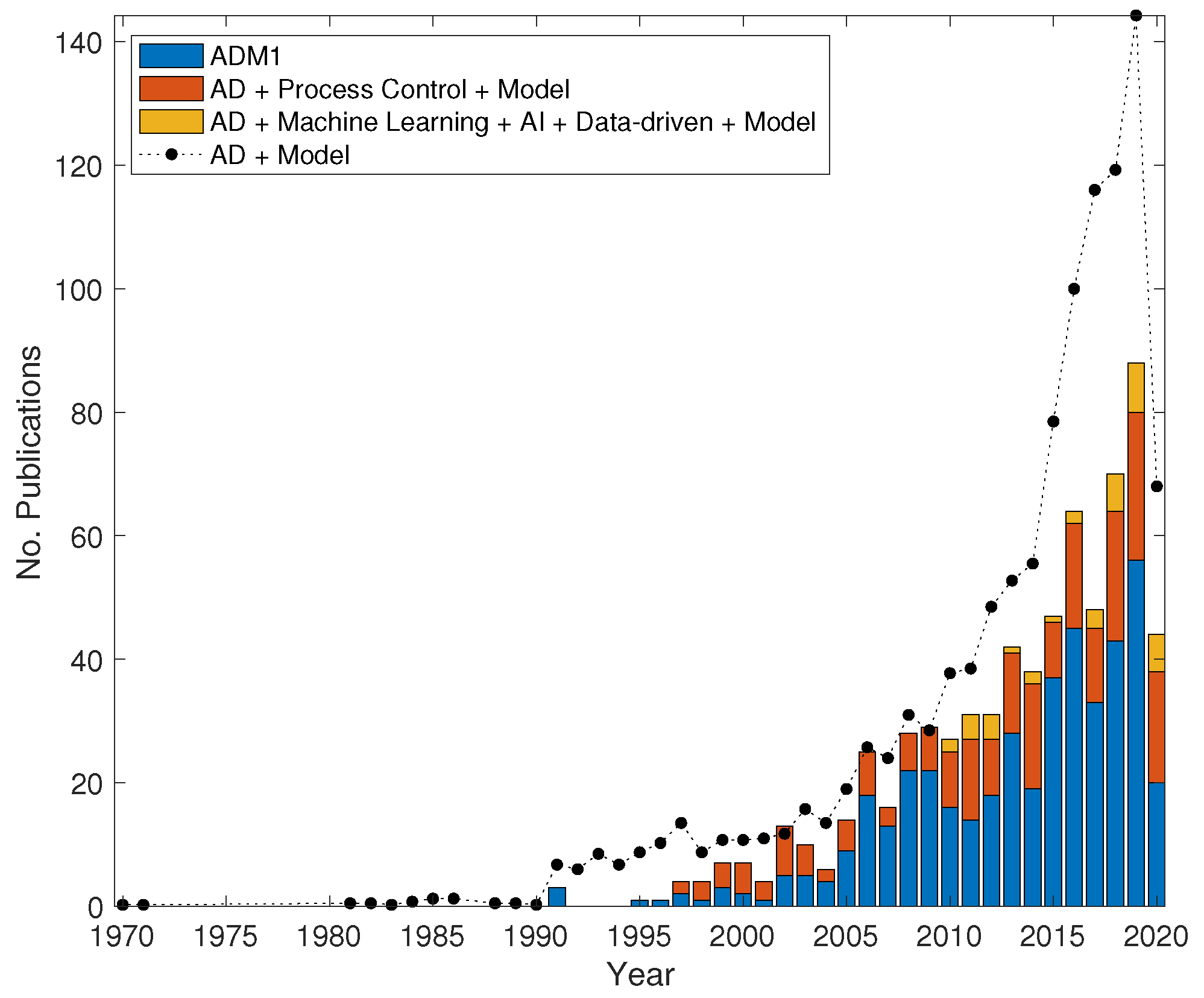
Figure 2.
A general schematic of the Gujer/Petersen matrix. We use to represent stoichiometric coefficients, for process rates and indicate the two commonly used constituents in biological treatment models, Chemical Oxygen Demand (COD) and nitrogen (N).
Figure 2.
A general schematic of the Gujer/Petersen matrix. We use to represent stoichiometric coefficients, for process rates and indicate the two commonly used constituents in biological treatment models, Chemical Oxygen Demand (COD) and nitrogen (N).
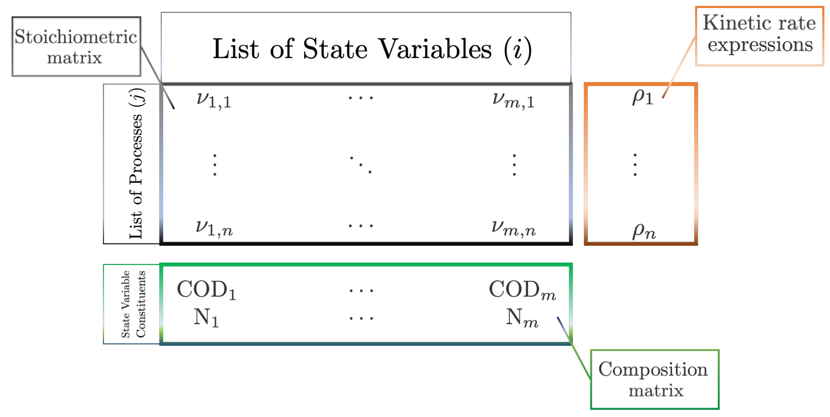
Figure 3.
Example of the thermodynamic ‘window of opportunity’ for syntrophic degradation of propionate via two pathways (MMC is the ‘classical’ methylmalonyl-CoA pathway). Both reactions are susceptible to hydrogen inhibition, shown by their increasing endergonicity as H partial pressure increases. Hydrogenotrophic methanogens mitigate this by transforming hydrogen to methane, above a certain partial pressure threshold required for growth. The red and blue boxes show the hydrogen partial pressures at which propionate degradation by the classical and Smithella pathways are possible due to this syntrophic behaviour (Adapted from [142]).

Figure 4.
Example of CFD modelling for a full-scale AD plant showing flow velocity and mixing profile within a stirred reactor. Image courtesy of AM-TEAM and BIOMATH (Ghent, Belgium, June 2020).
Figure 4.
Example of CFD modelling for a full-scale AD plant showing flow velocity and mixing profile within a stirred reactor. Image courtesy of AM-TEAM and BIOMATH (Ghent, Belgium, June 2020).

Figure 5.
An Individual-based Model representing the morphology of (top) A nitrifying-denitrifying biofilm. Ammonia Oxidising Bacteria (AOB) are seen to outcompete their Nitrite Oxidising counterparts (NOB) for dissolved oxygen in the bulk liquid (empty space). Competition for nitrite between ammonia oxidisers (ANA) and heterotrophs (HET) is observed within the biofilm, with HET establishing at the surface and ANA dominant in the anoxic regions of the biofilm, (bottom) An anaerobic digester. Morphology is dependent on initial seeding. The relative density of acetoclastic methanogens (xac_ch4) and hydrogenotrophic methanogens (xco2_ch4) is indicative of the dominant acetoclastic pathway, and the syntrophic interaction with the acetogens (xglu_ac). The images were produced using the NUFEB simulator [183] by Bowen Li (Newcastle University, UK, June 2020) and used with permission.


Table 1.
Important AD mathematical modelling milestones towards ADM1. Key (Process): EH = Enzymatic hydrolysis, AG = Acidogenesis, AGp = propionate Acidogenesis, AGb = butyrate Acidogenesis, AGa = acetate Acidogenesis, AcG = Acetogenesis, pAcG = propionate-degrading Acetogenesis, bAcG = butyrate-degrading Acetogenesis, fAcG = fatty acid-degrading Acetogenesis, AMG = Acetoclastic Methanogenesis, HMG = Hydrogenotrophic Methanogenesis; (Industry): = Agricultural, Biological (Activated) Sludge, General AD, Industrial Wastewater; (Program): CSMP = Continuous Systems modelling Program, NR = Dynamic solver/program not reported. Note. Number of parameters include conventional operating/control parameters such as dilution rate and influent concentrations. * Parameter information not available.
| Model | # State Variables | # Parameters | Year | Program | Notes | Reference |
|---|---|---|---|---|---|---|
| [AGa →AMG] | 9 | 28 | 1977 | CSMP | VFA and NH inhibition on MG only | [41] |
| [AGa →AMG + HMG] | 4 | N/A * | 1982 | CSMP | Complete use of H assumed | [45,46] |
| [AGp + AGb →AcG→AMG + HMG] | 9 | 18 | 1983 | NR | pH regulation through redox potential by H | [47] |
| [EH →AG→pAcG→AMG + HMG] | 10 | 35 | 1984 | MIMIC | First generalised and structured model (stoichiometric matrix) | [48] |
| [EH →AGa→AMG] | 7 | 14 | 1986 | NR | Hydrolysis of dead, particulate biomass is rate-limiting step | [49] |
| [AGa →AMG] | 5 | 23 | 1986 | NR | VFA inhibition on AG & MG, NH inhibition on MG | [50] |
| [EH → AG → pAcG + bAcG →AMG] | 16 | 33 | 1993 | Pascal | NH inhibition & pH-Temperature interactions | [51] |
| [EH →AG→pAcG + fAcG→AMG + HMG] | 18 | 48 | 1993 | Pascal | Extension of structured approach. Focus on acetate kinetics/digester stability | [52] |
| [EH →AGp + AGa→AcG + pSR + aSR→AMG + HMG] | 33 | 55 | 1994 | METHANE | H inhibition considered | [53] |
| [EH →AG→MG] | 5 | 14 | 1996 | TUTSIM | Reduced order for process control | [38] |
© 2020 by the author. Licensee MDPI, Basel, Switzerland. This article is an open access article distributed under the terms and conditions of the Creative Commons Attribution (CC BY) license (http://creativecommons.org/licenses/by/4.0/).
Share and Cite
MDPI and ACS Style
Wade, M.J. Not Just Numbers: Mathematical Modelling and Its Contribution to Anaerobic Digestion Processes. Processes 2020, 8, 888. https://0-doi-org.brum.beds.ac.uk/10.3390/pr8080888
AMA Style
Wade MJ. Not Just Numbers: Mathematical Modelling and Its Contribution to Anaerobic Digestion Processes. Processes. 2020; 8(8):888. https://0-doi-org.brum.beds.ac.uk/10.3390/pr8080888
Chicago/Turabian StyleWade, Matthew J. 2020. "Not Just Numbers: Mathematical Modelling and Its Contribution to Anaerobic Digestion Processes" Processes 8, no. 8: 888. https://0-doi-org.brum.beds.ac.uk/10.3390/pr8080888
Note that from the first issue of 2016, this journal uses article numbers instead of page numbers. See further details here.