Actuator and Sensor Fault Classification for Wind Turbine Systems Based on Fast Fourier Transform and Uncorrelated Multi-Linear Principal Component Analysis Techniques

Abstract

In response to the high demand of the operation reliability and predictive maintenance, health monitoring and fault diagnosis and classification have been paramount for complex industrial systems (e.g., wind turbine energy systems). In this study, data-driven fault diagnosis and fault classification strategies are addressed for wind turbine energy systems under various faulty scenarios. A novel algorithm is addressed by integrating fast Fourier transform and uncorrelated multi-linear principal component analysis techniques in order to achieve effective three-dimensional space visualization for fault diagnosis and classification under a variety of actuator and sensor faulty scenarios in 4.8 MW wind turbine benchmark systems. Moreover, comparison studies are implemented by using multi-linear principal component analysis with and without fast Fourier transform, and uncorrelated multi-linear principal component analysis with and without fast Fourier transformation data pre-processing, respectively. The effectiveness of the proposed algorithm is demonstrated and validated via the wind turbine benchmark.

1. Introduction

With the development of advanced technologies to increase production, modern industrial systems become more complex and expensive. The components of industrial systems are prone to malfunction, which could bring unanticipated economic costs due to unscheduled shutdown and repair/maintenance. Therefore, it is of particular interest to design effective fault diagnosis and fault classification approaches to automatically monitor the behaviour of industrial systems and prevent damage caused by unexpected faults. Motivated by environmental considerations and the shortage of fossil fuels, wind turbines, as one of renewable energy sources, have contributed to a large portion of the world’s power production [1,2]. As a clean energy, wind energy has been significantly exploited via the onshore and offshore wind turbines. By the end of 2019, the overall installation capacity of all wind turbines worldwide reached 651 GW, and European countries contributed to 205 GW. Moreover, wind power contributed 15% electricity generation in Europe and 20% electricity production in the UK in 2019 [3].

Wind farms consisting of hundreds of wind turbine units are being established in many different locations around the country, for instance, in offshore, arctic, and desert regions. In recent years, some different topologies of generators, such as doubly fed induction generators (DFIGs) and permanent magnet synchronous generators (PMSGs), are widely utilized in wind turbine systems. However, like any other industrial systems, wind turbines are sophisticated and prone to faults. It is observed that the operation and maintenance costs for onshore and offshore wind turbines make up 10~15% and 20~35%, respectively, of the total life costs of wind energy conversion systems. Furthermore, wind turbine systems are complex and expensive; therefore, there is a high demand for improving the reliability and availability, and reducing unscheduled down time in wind turbine industries [4]. Motivated by the above, monitoring and fault diagnosis for wind turbine systems have received wide attention in wind turbine industries [5,6,7,8,9].

Fault diagnosis approaches can be classified into model-based, signal-based, and knowledge-based methods. The model-based fault diagnosis approach requires a well-established model of practical processes developed by either physical principles or systems identification techniques. By checking the residual between the model output and the real-time process output, the decision for fault diagnosis can be made [10,11]. Signal-based fault diagnosis is relying on appropriate sensors, whose locations are normally installed in plant components. The faults in the process are reflected in the measured signals, and the time-domain, frequency-domain, or time-frequency-domain techniques are used to extract features. By checking the consistency between the features of the real-time process and the prior knowledge on the symptoms of the healthy system, a diagnostic decision can be made [12]. Knowledge-based approaches utilize a large volume of historic data available to train universal estimations or approximations on behalf of implementing to recognize faulty conditions [13]. It is worthy to point out that the knowledge-based approach more depends on the data processing and data-based learning, including processing historical data and real-time data. Therefore, the knowledge-based fault diagnosis approach is often called the data-driven approach [14,15].

Machine learning techniques play an important role for data-driven fault diagnosis. Generally speaking, machine learning techniques can mainly be classified into three categories, which are unsupervised, semi-supervised, and supervised learning algorithms, respectively [16]. Unsupervised machine learning aims to learn structure in the data, such as sparse or low-dimensional feature representation [17,18,19,20]. According to the tasks of the supervised machine learning, such as prediction and classification, the aim is to learn a knowledge base, on the basis of the known or labelled examples of the target pattern [21,22]. Semi-supervised machine learning represents a class of algorithms that include both supervised and unsupervised tasks [23,24,25].

It is noted that the dataset generally has a great volume of data with existence in high-dimensional space. Feature extractions thus play an important role in data-driven fault diagnosis [26,27,28,29] as well as dimensionality reduction for the samples/datasets. The geometric distribution of the datasets in high-dimensional space can be analyzed in order to effectively extract significant features. There are several methods to solve this problem and one of the most popular techniques is the principal component analysis (PCA) algorithm [30,31,32,33,34]. The PCA, as an unsupervised learning technique, is a statistical procedure that utilizes an orthogonal transformation to convert a set of correlated variables into linearly uncorrelated variables, namely principal components [35]. The number of principal components should be generally less than the number of the original variables [36,37,38]. The transformation in the PCA is carried out in a way so that the first principal component has the largest possible variance, and each succeeding component in turns has the highest variance possible under the constraint that it is orthogonal to the preceding components [39]. As a result, the PCA has become a popular tool for fault detection and fault classification on the basis of a large volume of high-dimensional experimental samples/datasets [40,41,42].

A wind turbine system is a complex industrial system, and the operation condition is harsh. Therefore, the conventional PCA technique may become invalid for fault diagnosis and fault classification in wind turbine systems subjected to multiple faults. As a result, there is a strong motivation to develop advanced PCA-based fault diagnosis and classification techniques for wind turbine systems. In this study, uncorrelated multi-linear principal component analysis (UMPCA) is integrated with FFT data preprocessing to form an algorithm, which is applied to a 4.8 MW wind turbine benchmark system for fault diagnosis and classification. Furthermore, comparison studies are carried out to demonstrate the effectiveness of the proposed algorithm by comparing with the known algorithms.

The rest of this paper is organized as follows: In Section 2, the fundamentals of the 4.8 MW wind turbine benchmark model are introduced, and actuator and sensor faults of wind turbines are explained. In Section 3, An algorithm integrated with FFT and UMPCA techniques is addressed for dimensionality reduction and feature extraction. Experimentation designs are proposed in terms of different topologies of the actuator and sensor faults of wind turbines in Section 4. Simulation studies are illustrated in Section 5. In order to demonstrate the effectiveness of the addressed FFT plus UMPCA method, the simulated studies of the fault diagnosis and classification for wind turbines respectively by using MPCA, FFT plus MPCA, and UMPCA are also discussed. Finally, this paper is ended by summarizing the conclusions in Section 6.

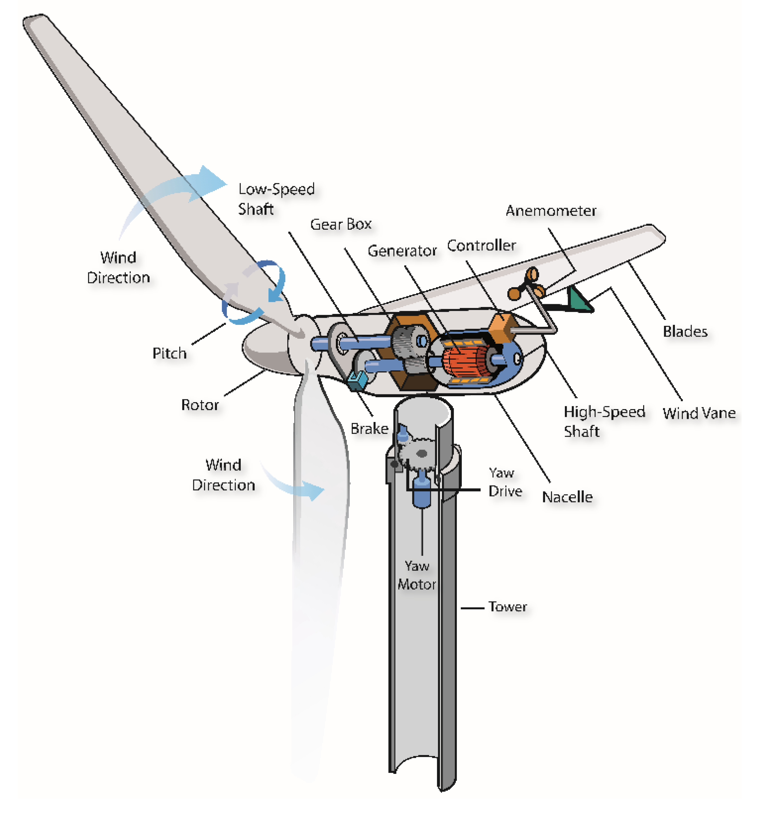
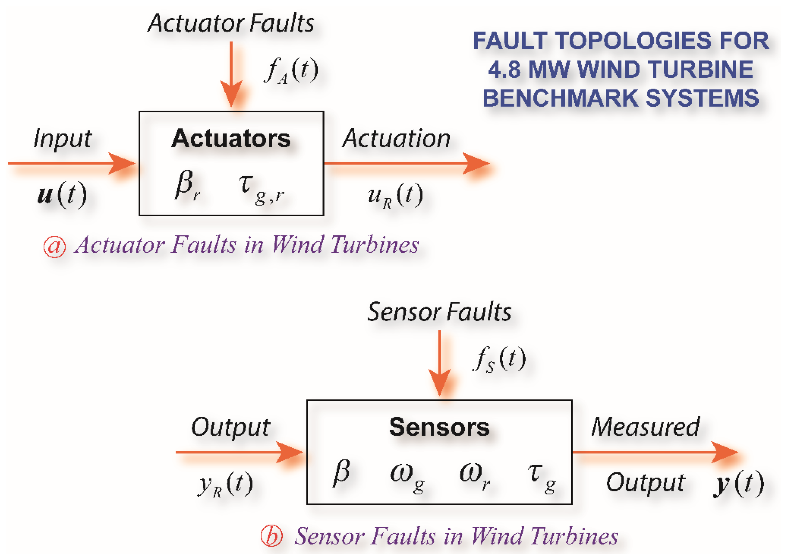
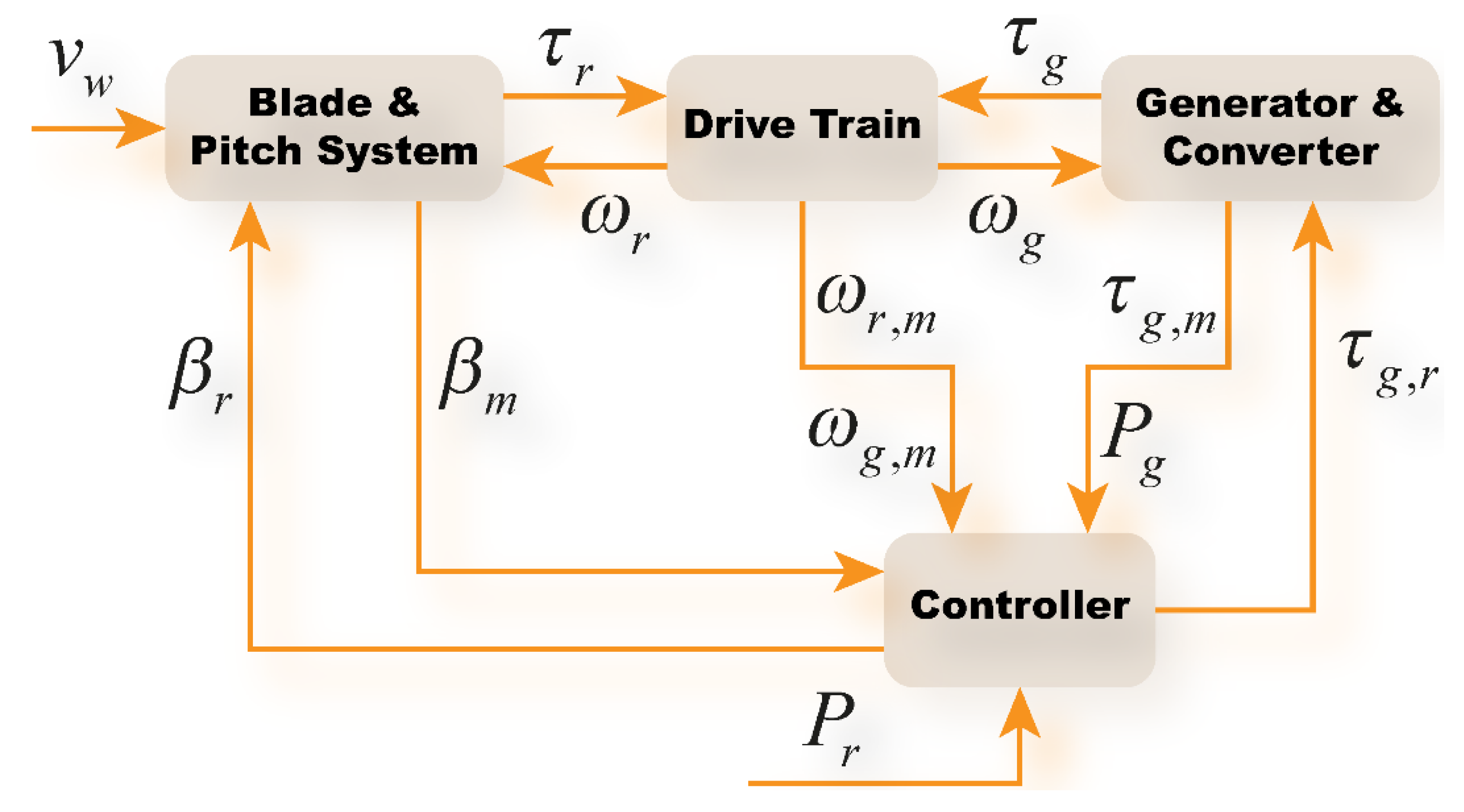
2. Wind Turbine Benchmark Systems

A wind turbine is a complex electro-mechanical system that converts wind energy to electrical energy. Most wind turbines are horizontal three–bladed unites, which are composed of blades, low-speed and high-speed shafts, gearbox, generator, yaw, tower, brake, and controller, and so forth. A typical structure of the wind turbine is depicted by Figure 1. The wind flow in the nature drives the blades and rotor to rotate, converting wind energy to mechanical energy. The rotor drives the generator via the high-speed shaft so that the mechanical energy is converted into electric energy. The pitch angle is controlled to adapt to the varying wind speed to achieve the desired output power. The functionality of the yaw system contributes to align the turbine with the direction of the wind detected by the anemometer.

A benchmark model of a 4.8 MW wind turbine system was developed in [43,44], which has been widely used for the algorithm validation in control and fault diagnosis. The definitions of the parameters of the benchmark model are shown in

Table 1. Parameters of the 4.8 MW wind turbine benchmark system [43,44].

Symbol	Definition	Symbol	Definition
${\beta }_r$	Pitch angle Reference	${\theta }_{\mathsf{\Delta }}$	Torsion Angle
${\tau }_{g,r}$	Generator Torque Reference	$\zeta$	Damping Ratio
$\beta$	Pitch Angle	$B_{dt}$	Torsion Damping Coefficient
${\omega }_g$	Generator Rotating Speed	$B_g$	Generator External Damping
${\omega }_r$	Rotor Angular Speed	$B_r$	Rotor External Damping
${\tau }_g$	Generator Torque	$C_q$	Torque Coefficient
${\alpha }_{gc}$	Generator and Converter Parameter	$J_g$	Generator Moment of Inertia
${\eta }_{dt}$	Efficiency of Drive Train	$J_r$	Rotor Moment of Inertia
$\lambda$	Tip-Speed-Ratio	$K_{dt}$	Torsion Stiffness
${\omega }_n$	Natural Frequency	$N_g$	Gear Ratio
$\rho$	Air Density	$R$	Rotor Radius

.

The diagram of the 4.8 MW wind turbine benchmark system is shown by Figure 2, which is composed of the blade and pitch subsystem, drive train subsystem, generator and convertor subsystem, and controller, respectively.

The wind turbine benchmark system has an external input (e.g., varying wind speed), two control reference inputs composed of the reference pitch angle (${\beta }_r$) and generator torque reference (${\tau }_{g,r}$).

The wind speed is shown in Figure 3, from which one can see the wind speed ranges from 5 to 20 m/s, with the peak spike over 25 m/s, showing a good coverage of the operation conditions under a healthy situation.

In this study, we focus on the actuator faults and sensor faults of the wind turbines. Suppose that $u\left(t\right)$ is the control input, $f_A\left(t\right)$ is the actuator fault, and $u_R\left(t\right)$ is the actuation signal applied to the system; $y\left(t\right)$ is the measured output, $f_S\left(t\right)$ is the sensor fault, and $y_R\left(t\right)$ is the output from the system. It is clear that $u_R\left(t\right)=u\left(t\right)+f_A\left(t\right),$ and $y\left(t\right)=y_R\left(t\right)+f_S\left(t\right)$. As a result, the faults $f_A\left(t\right)$ and $f_S\left(t\right)$ will divert the performance of the system states and outputs from the normal. The topologies of the actuator faults and sensor faults are depicted by Figure 4.

3. Methodology

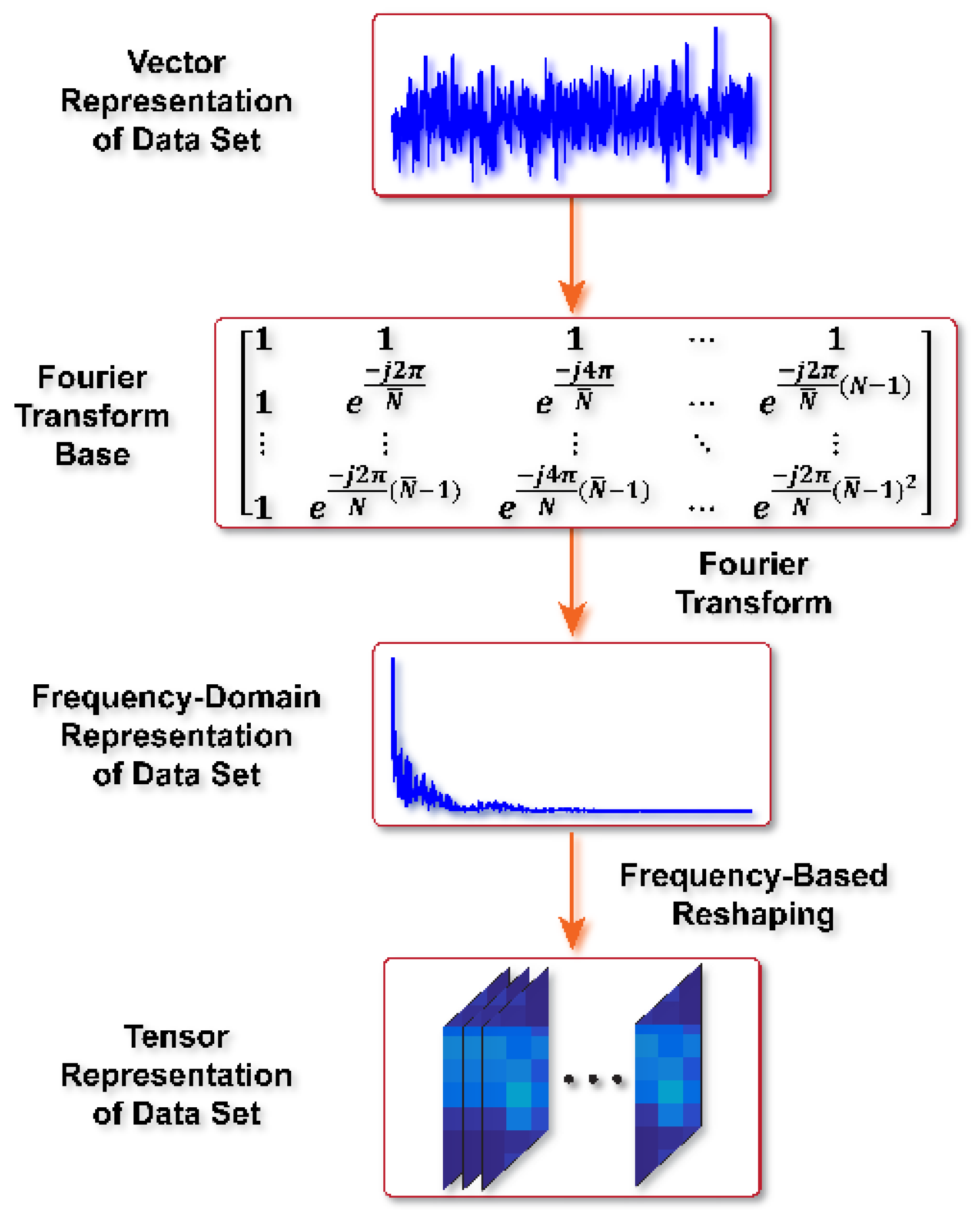
3.1. Data Set Construction

The 4.8 MW wind turbine benchmark system has four measurement outputs, namely the pitch angle $\beta$, the generator rotating speed ${\omega }_g$, the rotor angular speed ${\omega }_r$, and generator torque ${\tau }_g$. By using the measurement outputs above, the data set recorded from each measurement, denoted by ${\beta }_s, {\omega }_{gs}, {\omega }_{rs},$ and ${\tau }_{gs}$, can be obtained as follows:

$$\begin{array}{cc} {\beta }_s=\left[\begin{array}{cccc}{\beta }_{s11}& {\beta }_{s12}& \cdots & {\beta }_{s1\gamma }\\ {\beta }_{s21}& {\beta }_{s22}& \cdots & {\beta }_{s2\gamma }\\ ⋮& ⋮& \ddots & ⋮\\ {\beta }_{sN1}& {\beta }_{sN2}& \cdots & {\beta }_{sN\gamma }\end{array}\right]\in R^{N\times \gamma }, & {\omega }_{gs}=\left[\begin{array}{cccc}{\omega }_{gs11}& {\omega }_{gs12}& \cdots & {\omega }_{gs1\gamma }\\ {\omega }_{gs21}& {\omega }_{gs22}& \cdots & {\omega }_{gs2\gamma }\\ ⋮& ⋮& \ddots & ⋮\\ {\omega }_{gsN1}& {\omega }_{gsN2}& \cdots & {\omega }_{gsN\gamma }\end{array}\right]\in R^{N\times \gamma }\\ {\omega }_{rs}=\left[\begin{array}{cccc}{\omega }_{rs11}& {\omega }_{rs12}& \cdots & {\omega }_{rs1\gamma }\\ {\omega }_{rs21}& {\omega }_{rs22}& \cdots & {\omega }_{rs2\gamma }\\ ⋮& ⋮& \ddots & ⋮\\ {\omega }_{rsN1}& {\omega }_{rsN2}& \cdots & {\omega }_{rsN\gamma }\end{array}\right]\in R^{N\times \gamma },& {\tau }_{gs}=\left[\begin{array}{cccc}{\tau }_{gs11}& {\tau }_{gs12}& \cdots & {\tau }_{gs1\gamma }\\ {\tau }_{gs21}& {\tau }_{gs22}& \cdots & {\tau }_{gs2\gamma }\\ ⋮& ⋮& \ddots & ⋮\\ {\tau }_{gsN1}& {\tau }_{gsN2}& \cdots & {\tau }_{gsN\gamma }\end{array}\right]\in R^{N\times \gamma }\end{array}$$

(1)

where $N$ is the number of the measurement points recorded, and $\gamma$ is the number of the measurement scenarios. Specifically, for each measurement output, the dataset is recorded under $\gamma$ operation scenarios (including the fault-free condition, and various faulty conditions), and $N$ measurement points are documented at each scenario. As a result, the original data set can be described by:

$$X=\left[\begin{array}{c}{\beta }_s\\ {\omega }_{gs}\\ {\omega }_{rs}\\ {\tau }_{gs}\end{array}\right]\in R^{\overline{N}\times \gamma },$$

(2)

where $\overline{N}=4N.$

3.2. Data Set Pre-Processing

In order to enhance the feature extraction capability, the time-domain data is pre-proceeded to generate frequency-domain data with a reshaping expression.

According to the original data-set model $X$ defined in (2), we can rewrite it as:

$$X=\left[\begin{array}{cccc}{X}_1& X_2& \cdots & X_{\gamma }\end{array}\right]=\left[\begin{array}{cccc}{x}_{11}& x_{12}& \cdots & x_{1\gamma }\\ x_{21}& x_{22}& \cdots & x_{2\gamma }\\ ⋮& ⋮& \ddots & ⋮\\ x_{\overline{N}1}& x_{\overline{N}2}& \cdots & x_{\overline{N}\gamma }\end{array}\right],$$

(3)

where $X_i={\left[\begin{array}{cccc}{x}_{1i}& x_{2i}& \cdots & x_{\overline{N}i}\end{array}\right]}^T$, $i=1, 2, \cdots , \gamma ,$and ${[·]}^T$ represents the transpose of the vector $[·].$

The Fourier transform of $X_i$ can be calculated as follows:

$$X_i\left(k\right)={{\displaystyle \sum }}_{t=1}^{\overline{N}}{x}_{ti}{e}^{\frac{-j2\pi }{\overline{N}}k\left(t-1\right)},$$

(4)

where $k=0, 1, 2, \cdots , \overline{N}-1$.

In terms of (4), the discrete-time Fourier transform can transform a sequence of $\overline{N}$numbers $\begin{array}{cccc}{x}_{1i}& x_{2i}& \cdots & x_{\overline{N}i}\end{array}$ into a sequence of complex numbers $X_i\left(0\right), X_i\left(1\right), \cdots , X_i\left(\overline{N}-1\right)$, which can also be denoted by the symbols $f_i^{\left(1\right)},f_i^{\left(2\right)}, \cdots , f_i^{\left(\overline{N}\right)}.$ By arranging the sequence of the complex numbers as a vector, we have:

$$\left[\begin{array}{c}{X}_i\left(0\right)\\ X_i\left(1\right)\\ \begin{array}{c}⋮\\ X_i\left(\overline{N}-1\right)\end{array}\end{array}\right]=\mathsf{\Omega }\left[\begin{array}{c}{x}_{1i}\\ x_{2i}\\ \begin{array}{c}{x}_{3i}\\ ⋮\\ x_{\overline{N}i} \end{array}\end{array}\right]:=\left[\begin{array}{c}{f}_i^{\left(1\right)}\\ f_i^{\left(2\right)}\\ \begin{array}{c}⋮\\ f_i^{\left(\overline{N}\right)}\end{array}\end{array}\right],$$

(5)

where:

$$\mathsf{\Omega }=\left[\begin{array}{ccccc}1& 1& 1& \cdots & 1\\ 1& e^{\frac{-j2\pi }{\overline{N}}}& e^{\frac{-j4\pi }{\overline{N}}}& \cdots & e^{\frac{-j2\left(\overline{N}-1\right)\pi }{\overline{N}}}\\ ⋮& ⋮& ⋮& \ddots & ⋮\\ 1& e^{\frac{-j2\left(\overline{N}-1\right)\pi }{\overline{N}}}& e^{\frac{-j4\left(\overline{N}-1\right)\pi }{\overline{N}}}& \cdots & e^{\frac{-j2{\left(\overline{N}-1\right)}^2\pi }{\overline{N}}}\end{array}\right],$$

(6)

and $\mathsf{\Omega }$ is called the Fourier transform base. It is clear that $i=1, 2, \cdots , \gamma$ in (5).

The Fourier transform above can be calculated by using the fast Fourier transform algorithm [45,46]. The fast Fourier transform algorithm treats the columns of a matrix as vectors and returns the Fourier transform vector for each column, leading to a Fourier transform matrix.

Taking magnitude and reshaping the vector in (5), one can obtain the matrix expression as follows:

$${\mathit{F}}_{\mathit{i}}=\left[\begin{array}{cccc}\left|f_i^{\left(1\right)}\right|& \left|f_i^{\left(r+1\right)}\right|& \cdots & \left|f_i^{\left(\left(l-1\right)r+1\right)}\right|\\ \left|f_i^{\left(2\right)}\right|& \left|f_i^{\left(r+2\right)}\right|& \cdots & \left|f_i^{\left(\left(l-1\right)r+2\right)}\right|\\ ⋮& ⋮& \ddots & ⋮\\ \left|f_i^{\left(r\right)}\right|& \left|f_i^{\left(2r\right)}\right|& \cdots & \left|f_i^{\left(\overline{N}\right)}\right|\end{array}\right]\in R^{r\times l}, i=1, 2, \cdots , \gamma ,$$

(7)

where $r$ indicates the number of rows, $l$ stands for the number of columns, $\left|(·)\right|$ represents the absolute value or magnitude of the complex number $(·),$ and $\overline{N}=lr.$ By determining two parameters $r$ and $l$, the frequency-domain data of the wind turbine can be described as follows:

$$\left\{\mathcal{F} | \mathcal{F}=\left[{\mathit{F}}_1, {\mathit{F}}_2,\dots ,{\mathit{F}}_{\mathit{i}},\dots , {\mathit{F}}_{\mathit{\gamma }}\right]\right\}\in R^{r\times l\times \gamma }.$$

(8)

Therefore, the dataset has been reformatted as a tensor data expression. From (8), one can see the dataset has $\gamma$ samples, and the size of each sample is $r\times l.$

The reshaping process of the obtained data set above can be described by the flowchart in Figure 5. From this figure, one can see the data vector (e.g., $X_i={\left[\begin{array}{cccc}{x}_{1i}& x_{2i}& \cdots & x_{\overline{N}i}\end{array}\right]}^T$, $i=1, 2, \cdots , \gamma$) is projected into a frequency-domain space relying on the Fourier transform base, and the tensor representation is further generated in terms of (7) and (8).

3.3. Dimensionality Reduction and Feature Extraction for Wind Turbines by Using the Uncorrelated Multi-Linear Principal Component Analysis Method

The multi-linear principal component analysis (MPCA) technique [47], which belongs to one of the unsupervised machine learning algorithms, is usually to cope with the tensor expression dataset. However, some of the correlations of the principal components amongst the projected directions are neglected to some extent, which means the final features obtained by MPCA would be redundant. In contrast to other multilinear PCA techniques, such as MPCA, two-dimensional PCA, and so forth, UMPCA seeks a tensor-to-vector projection, which can capture the maximum number of the uncorrelated multilinear features [39,48]. In this paper, UMPCA is thus used to extract the significant features of the 4.8 MW benchmark wind turbines.

The $n$-mode product of a tensor $\mathcal{F}$ by a matrix $U$is denoted by $\mathcal{F}{\times }_{n}U$ [39,48].

Suppose the dataset $\left\{{\mathit{z}}_i\left(p\right), i=1, 2,\dots , \gamma \right\}$ represents the $p$th principal components (e.g., low-dimensional features), where ${\mathit{z}}_i\left(p\right)$ is the projection of the $i\mathrm{th}$ data sample ${\mathit{F}}_i$ by the p-th elementary multi-linear projection (EMP) $U_p=\left\{{\left({\mathit{u}}_p^{\left(n\right)}\right)}^T, n=1, 2,\dots , Q\right\}$, where $Q$ represents the number of projection directions. As a result, the formula of ${\mathit{z}}_i\left(p\right)$ can be described as follows [39,48]:

$${\mathit{z}}_i\left(p\right)={\mathit{F}}_i{\times }_{n=1}^Q\left\{{\left({\mathit{u}}_p^{\left(n\right)}\right)}^T, n=1, 2,\dots , Q\right\}, i=1, 2,\dots , \gamma .$$

(9)

The objective of the UMPCA methodology is to seek $U_p$ that projects ${\mathit{F}}_i$ into a feature subspace to determine a tensor-to-vector projection, whose functionality will guarantee the implementation for the maximum direction of the original data sets, and the significant features extracted are uncorrelated. Based on the above, the variance can be calculated by [39,48]:

$${\mathcal{S}}_{T_p}^{\mathit{z}}={{\displaystyle \sum }}_{i=1}^{\gamma }{\left[{\mathit{z}}_i\left(p\right)-{\overline{z}}_p\right]}^2,$$

(10)

where ${\overline{z}}_p={\displaystyle \sum }_{i=1}^{\gamma }\frac{z_i\left(p\right)}{\gamma }.$ Let $h_p$ denote the $p$th coordinate vector, describing the training sample in the pth EMP space. The ith component of $h_p$ equals the p-th component of ${\mathit{z}}_i,$ that is, $h_p\left(i\right)=z_i\left(p\right).$

In order to determine a set of projection directions $U_p=\left\{{\left({\mathit{u}}_p^{\left(n\right)}\right)}^T, n=1, 2,\dots , Q\right\}$ to maximize the variance and generate uncorrelated features, the cost function can be given as follows [39,48]:

$$\begin{array}{c}\left\{{\left({\mathit{u}}_p^{\left(n\right)}\right)}^T, n=1, 2,\dots , Q\right\}=\arg max{\mathcal{S}}_{T_p}^z\\ s.t.{\left\{{\mathit{u}}_p^{\left(n\right)}\right\}}^T·{\mathit{u}}_p^{\left(n\right)}=1, \mathrm{and} \frac{{\left({\mathit{h}}_p\right)}^T{h}_q}{||{\mathit{h}}_p||·||{\mathit{h}}_q||}={\delta }_{pq}, \left(p,q=1, 2,\dots , P\right),\end{array}$$

(11)

where $P$ is the dimensionality of the projected space, and:

$${\delta }_{pq}=\{\begin{array}{c}1, if p=q\\ 0, otherwise.\end{array}$$

(12)

In terms of the background of the benchmark wind turbine in Section 2 and the fundamental principle of the UMPCA [39,48] mentioned above, the specific procedures of the significant feature extraction for wind turbines can be illustrated as follows.

Step 1:

Explore the first projection direction $U_1=\left\{{\left({\mathit{u}}_1^{\left(n\right)}\right)}^T, n=1, 2,\dots , Q\right\}$ by maximizing ${\mathcal{S}}_{T_1}^z$.

Step 2:

Compute the second project direction $u_2=\left\{{\left({\mathit{u}}_2^{\left(n\right)}\right)}^T, n=1, 2,\dots , Q\right\}$ by maximizing ${\mathcal{S}}_{T_2}^z$ subjected to $h_2^T{h}_1=0$.

Step 3:

Determine the third project direction $u_3=\left\{{\left({\mathit{u}}_3^{\left(n\right)}\right)}^T, n=1, 2,\dots , Q\right\}$ by maximizing ${\mathcal{S}}_{T_3}^z$subjected to $h_3^T{h}_2=0$.

Step 4:

Calculate the p-th project direction $u_p=\left\{{\left({\mathit{u}}_p^{\left(n\right)}\right)}^T, n=1, 2,\dots , Q\right\},$ $p=4, \cdots , P,$ by maximizing ${\mathcal{S}}_{T_p}^z$ subjected to $h_p^T{h}_q=0,$when $q=1, 2, \cdots , p-1$.

Step 5:

Based on all the obtained project directions from the steps above, the final features can be obtained by:

$$z_i={\mathit{F}}_i{\times }_{n=1}^Q{\left\{{\left({\mathit{u}}_p^{\left(n\right)}\right)}^T, n=1, 2,\dots , Q\right\}}_{p=1}^P, i=1, 2,\dots , \gamma .$$

(13)

3.4. FFT Plus UMPCA Algorithm

The specific procedures of the dimensionality reduction and feature extraction based on FFT plus the UMPCA technique for wind turbines can be described as follows:

Algorithm 1

Input: Date set $\left\{\mathcal{F} | \mathcal{F}=\left[{\mathit{F}}_{\mathbf{1}}, {\mathit{F}}_{\mathbf{2}},\dots ,{\mathit{F}}_{\mathbf{i}},\dots , {\mathit{F}}_{\mathit{\gamma }}\right]\right\}$. Output: Significant features ${\mathit{z}}_i={\mathit{F}}_i{\times }_{n=1}^Q{\left\{{\left({\mathit{u}}_p^{\left(n\right)}\right)}^T, n=1, 2,\dots , Q\right\}}_{p=1}^P, i=1, 2,\dots , \gamma$.   (i) Step 1: Collect the original data set X by (2)   (ii) Step 2: Pre-process the data set by using Fourier transform base to construct the tensor dataset by (7) and (8).   (iii) Step 3: Calculate the projection directions $U_1, U_2, \cdots , U_P$;   (iv) Step 4: Project the FFT data space into a vector subspace by using ${\mathit{z}}_i={\mathit{F}}_i{\times }_{n=1}^Q{\left\{{\left({\mathit{u}}_p^{\left(n\right)}\right)}^T, n=1, 2,\dots , Q\right\}}_{p=1}^P, i=1, 2,\dots , \gamma$. As a result, for the tensor dataset $\mathcal{F},$ the resultant UMPCA feature vector z can be given as $\mathit{z}=\mathcal{F}{\times }_{n=1}^Q{\left\{{\left({\mathit{u}}_p^{\left(n\right)}\right)}^T, n=1, 2,\dots , Q\right\}}_{p=1}^P$.

4. Experimentation Designs

4.1. Brief Description and Definition

In this section, in order to validate the applicability of the proposed methodology for fault diagnosis and fault classification in wind turbine systems, five different topologies of experimentation are addressed subsequently. Furthermore, actuator and sensor faults are simultaneously considered in each group of experiment. The size of each data set is $1000\times 440,001$.

For the simplicity of the description for the subsequent experimentations, we define some abbreviations for different types of faulty conditions in two actuators and four sensors. ‘A1′ represents the first actuator relevant to the pitch angle reference (${\beta }_r$); ‘A2′ stands for the second actuator relevant to the generator torque reference (${\tau }_{g,r}$); ‘S1′ is the first sensor to measure the pitch angle ($\beta$), ‘S2’ indicates the second sensor to measure the generator rotating speed (${\omega }_g$), ‘S3′ stands for the third sensor to measure the rotor angular speed (${\omega }_r$), and ‘S4’ defines as the fourth sensor to measure the generator torque (${\tau }_g$). The detailed information is shown in

Table 2. Symbols and acronyms of the actuator and sensor for 4.8 MW wind turbines.

	Actuator		Sensor
Symbol	${\beta }_r$	${\tau }_{g,r}$	$\beta$	${\omega }_g$	${\omega }_r$	${\tau }_g$
Acronym	A1	A2	S1	S2	S3	S4

.

In addition, ‘FF’ indicates fault free. ‘EL’, ‘SWD’, and ‘RN’ represent effectiveness losses, sinusoidal wave disturbances, and random numbers, respectively. Their combination, including ‘EL + SWD’, ‘EL + RN’, ‘SWD + RN’, and ‘EL + SWD + RN’, are also taken into consideration.

The other abbreviations of the parameters for faulty signals are defined as follows, whose specifications are explained in

Table 3. Operation Conditions, Parameters, and Acronyms for 4.8 MW Wind Turbine Systems.

Operation Conditions	Abbreviations	Parameters	Acronyms
Fault Free	FF	-	-
Effectiveness Losses	EL	Percentage	P
Sinusoidal Wave Disturbances	SWD	Amplitude & Bias	A/B
Random Numbers	RN	Mean & Variance	M/V
Effectiveness Losses + Sinusoidal Wave Disturbances	EL + SWD	Percentage + Amplitude + Bias	P/A/B
Effectiveness Losses + Random Numbers	EL + RN	Percentage + Mean + Variance	P/M/V
Sinusoidal Wave Disturbances + Random Numbers	SWD + RN	Amplitude + Bias + Mean + Variance	A/B/M/V
Effectiveness Losses + Sinusoidal Wave Disturbances + Random Numbers	EL + SWD + RN	Amplitude + Bias + Mean + Variance	P/A/B/M/V

:

(1)

‘EL’: Percentage (P);

(2)

‘SWD’: Amplitude (A) and Bias (B), namely A/B

(3)

‘RN’: Mean (M), and Variance (V), namely M/V;

(4)

‘EL + SWD’: Percentage (P), Amplitude (A), and Bias (B), namely P/A/B;

(5)

‘EL + RN’: Percentage (P), Mean (M), and Variance (V), namely P/M/V;

(6)

‘SWD + RN’: Amplitude (A), Bias (B), Mean (M), and Variance (V), namely A/B/M/V;

(7)

‘EL + SWD + RN’: Percentage (P), Amplitude (A), Bias (B), Mean (M), and Variance (V), namely P/A/B/M/V.

4.2. Experimental Statement

In the experiment, the fault signals are shown in

Table 4. Actuator and sensor fault signals: Experimentation design.

Faulty Conditions	Name of Parameters	Actuator and Sensor Faults
		Actuator		Sensor
		${\mathit{\beta }}_{\mathit{r}}$	${\mathit{\tau }}_{\mathit{g},\mathit{r}}$	$\mathit{\beta }$	${\mathit{\omega }}_{\mathit{g}}$	${\mathit{\omega }}_{\mathit{r}}$	${\mathit{\tau }}_{\mathit{g}}$
EL	P	1.00–20.00%
SWD	A	0.01–0.20	5.20–9.00	0.01–0.20	5.20–9.00	0.01–0.20	5.20–9.00
	B	0.10–2.00	501–520	0.10–2.00	50.10–52.00	0.01–0.20	501–520
RN	M	0.10–2.00	1.00–20.00	0.10–2.00	1.00–20.00	0.01–0.20	1.00–20.00
	V	0.20–2.10	91.00–110.00	0.20–2.10	1.10–2.05	0.01–0.20	91.00–110.00
EL + SWD	P/A/B	${\beta }_r$: P/A/B—From 1.00%/0.01/0.10 to 20.00%/0.20/2.00;
		${\tau }_{g,r}$: P/A/B—From 1.00%/5.20/501 to 20.00%/9.00/520;
		$\beta$: P/A/B—From 1.00%/0.01/0.10 to 20.00%/0.20/2.00;
		${\omega }_g$: P/A/B—From 1.00%/5.20/50.10 to 20.00%/9.00/52.00;
		${\omega }_r$: P/A/B—From 1.00%/0.01/0.01 to 20.00%/0.20/0.20;
		${\tau }_g$: P/A/B—From 1.00%/5.20/501 to 20.00%/9.00/520.
EL + RN	P/M/V	${\beta }_r$: P/M/V—From 1.00%/0.10/0.20 to 20.00%/2.00/2.10;
		${\tau }_{g,r}$: P/M/V—From 1.00%/1.00/91 to 20.00%/20.00/110;
		$\beta$: P/M/V—From 1.00%/0.10/0.20 to 20.00%/2.00/2.10;
		${\omega }_g$: P/M/V—From 1.00%/1.00/1.10 to 20.00%/20.00/2.05;
		${\omega }_r$: P/M/V—From 1.00%/0.01/0.01 to 20.00%/0.20/0.20;
		${\tau }_g$: P/M/V—From 1.00%/1.00/91 to 20.00%/20.00/110.
SWD + RN	A/B/M/V	${\beta }_r$: A/B/M/V—From 0.01/0.10/0.10/0.20 to 0.20/2.00/2.00/2.10;
		${\tau }_{g,r}$: A/B/M/V—From 5.20/501/1.00/91 to 9.00/520/20.00/110;
		$\beta$: A/B/M/V—From 0.01/0.10/0.10/0.20 to 0.20/2.00/2.00/2.10;
		${\omega }_g$: A/B/M/V—From 5.20/50.10/1.00/1.10 to 9.00/52.00/20.00/2.05;
		${\omega }_r$: A/B/M/V—From 0.01/0.01/0.01/0.01 to 0.20/0.20/0.20/0.20;
		${\tau }_g$: A/B/M/V—From 5.20/501/1.00/91 to 9.00/520/20.00/110.
EL + SWD + RN	P/A/B/M/V	${\beta }_r$: P/A/B/M/V—From 1.00%/0.01/0.10/0.10/0.20
		to 20.00%/0.20/2.00/2.00/2.10;
		${\tau }_{g,r}$: P/A/B/M/V—From 1.00%/5.20/501/1.00/91
		to 20.00%/9.00/520/20.00/110;
		$\beta$: P/A/B/M/V—From 1.00%/0.01/0.10/0.10/0.20
		to 20.00%/0.20/2.00/2.00/2.10;
		${\omega }_g$: P/A/B/M/V—From 1.00%/5.20/501/1.00/1.10
		to 20.00%/9.00/52.00/20.00/2.05;
		${\omega }_r$: P/A/B/M/V—From 1.00%/0.01/0.01/0.01/0.01
		to 20.00%/0.20/0.20/0.20/0.20;
		${\tau }_g$: P/A/B/M/V—From 1.00%/5.20/501/1.00/91
		to 20.00%/9.00/520/20.00/110.

Supplementary Explanations: (i). AWGN signals are introduced to each faulty condition, and the number of AWGN signals is equal to 50; (ii). For ${\beta }_r$, the EL is increased from 1.00 to 20.00% with an increase of 1.00%, and the Amplitude of the SWD increases from 0.01 to 0.20 with an increase by 0.01, and the Bias varies between 0.10 and 2.00 with the interval of 0.10, gradually, as well as the Mean of RN increases from 0.01 to 0.20 with an increase by 0.01, and the Variance increases between 0.20 and 2.10 with the interval of 0.10.

. For instance, the effective loss (EL) of every single actuator or sensor is selected as 1%, 2%, 3%, …, 19% and 20% of the normal value, respectively, which means there are 20 faulty cases for the typical fault EL. More detailed information on other faults can refer to Table 4.

In this section, five groups of experiments of multiple actuator and sensor faults are discussed:

(i)

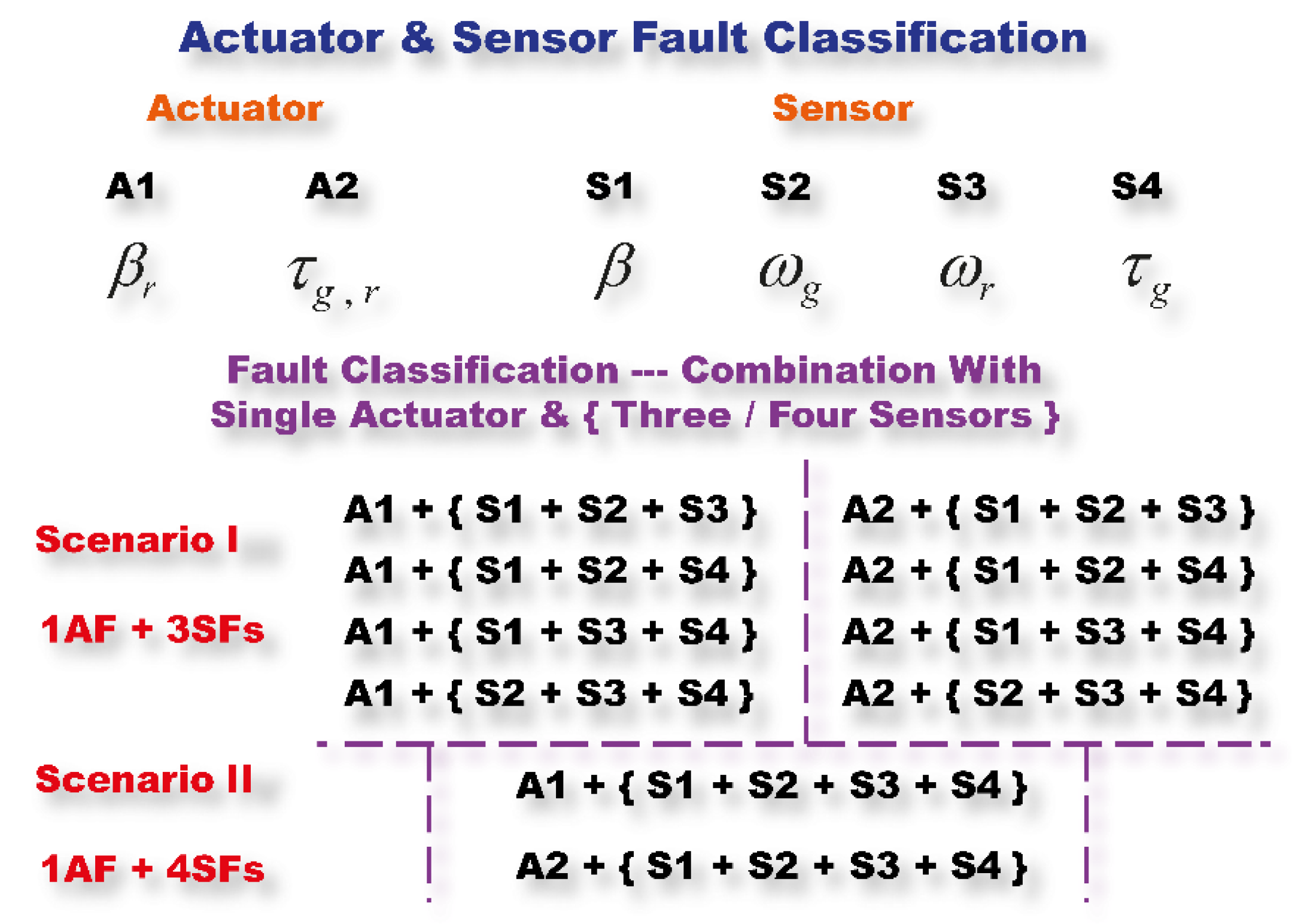
Scenario I: single actuator and three sensor faults, ‘1AF + 3SFs’; Types of fault: $C_2^1\cdot C_4^3=8$;

(ii)

Scenario II: single actuator and four sensor faults, ‘1AF + 4SFs’; Types of fault: $C_2^1\cdot C_4^4=2$;

(iii)

Scenario III: two actuators and two sensor faults, ‘2AFs + 2SFs’; Types of fault: $C_2^2\cdot C_4^2=6$;

(iv)

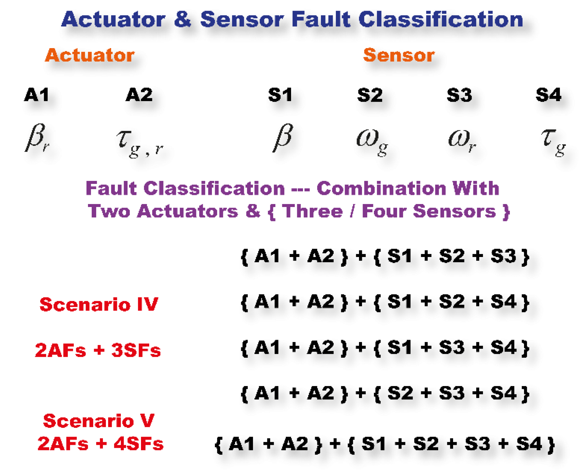
Scenario IV: two actuators and three sensor faults, ‘2AFs + 3SFs’; Types of fault: $C_2^2\cdot C_4^3=4$;

(v)

Scenario V: two actuators and four sensor faults, ‘2AFs + 4SFs’; Types of fault: $C_2^2\cdot C_4^4=1$.

These scenarios are further illustrated by Figure 6, Figure 7 and Figure 8. From Figure 6, one can see there are eight combinations of actuator and sensor faults under Scenario I, and two combinations in Scenario II. Figure 7 describes Scenario III and Figure 8 explains Scenarios IV and V, respectively.

In order to evaluate the feasibility and capability of the proposed FFT + UMPCA algorithm, the MPCA, UMPCA, and FFT + MPCA techniques are also discussed and analyzed. The datasets of the experiments using the algorithms MPCA, UMPCA, FFT + MPCA, and FFT + UMPCA, respectively, are shown in

Table 5. Datasets of experimentations with AWGN noises based on different topologies of the data-driven methodologies: MPCA and UMPCA.

Name of Experimentation	Types	Data Sets with AWGN Noises Based on Different Topologies of Data-Driven Methodologies
		MPCA	UMPCA
FF + 1AF + 3SFs	9	${\mathit{X}}_{\mathrm{I}}^{MPCA}\in R^{\left\{440,000\times 4\times 9000\right\}}$	${\mathit{X}}_{\mathrm{I}}^{UMPCA}\in R^{\left\{22,000\times 80\times 9000\right\}}$
FF + 1AF + 4SFs	3	${\mathit{X}}_{\mathrm{II}}^{MPCA}\in R^{\left\{440,000\times 4\times 3000\right\}}$	${\mathit{X}}_{\mathrm{II}}^{UMPCA}\in R^{\left\{22,000\times 80\times 3000\right\}}$
FF + 2AFs + 2SFs	7	${\mathit{X}}_{\mathrm{III}}^{MPCA}\in R^{\left\{440,000\times 4\times 7000\right\}}$	${\mathit{X}}_{\mathrm{III}}^{UMPCA}\in R^{\left\{22,000\times 80\times 7000\right\}}$
FF + 2AFs + 3SFs	5	${\mathit{X}}_{\mathrm{IV}}^{MPCA}\in R^{\left\{440,000\times 4\times 5000\right\}}$	${\mathit{X}}_{\mathrm{IV}}^{UMPCA}\in R^{\left\{22,000\times 80\times 5000\right\}}$
FF + 2AFs + 4SFs	2	${\mathit{X}}_{\mathrm{V}}^{MPCA}\in R^{\left\{440,000\times 4\times 2000\right\}}$	${\mathit{X}}_{\mathrm{V}}^{UMPCA}\in R^{\left\{22,000\times 80\times 2000\right\}}$

and

Table 6. Datasets of experimentations with AWGN noises based on different topologies of the data-driven methodologies: FFT + MPCA and FFT + UMPCA.

Name of Experimentation	Types	Data Sets with AWGN Noises Based on Different Topologies of Data-Driven Methodologies
		FFT + MPCA	FFT + UMPCA
FF + 1AF + 3SFs	9	${\mathit{X}}_{\mathrm{I}}^{FFT+MPCA}\in R^{\left\{550\times 800\times 4\times 9000\right\}}$	${\mathit{X}}_{\mathrm{I}}^{FFT+UMPCA}\in R^{\left\{100\times 220\times 80\times 9000\right\}}$
FF + 1AF + 4SFs	3	${\mathit{X}}_{\mathrm{II}}^{FFT+MPCA}\in R^{\left\{550\times 800\times 4\times 3000\right\}}$	${\mathit{X}}_{\mathrm{II}}^{FFT+UMPCA}\in R^{\left\{100\times 220\times 80\times 3000\right\}}$
FF + 2AFs + 2SFs	7	${\mathit{X}}_{\mathrm{III}}^{FFT+MPCA}\in R^{\left\{550\times 800\times 4\times 7000\right\}}$	${\mathit{X}}_{\mathrm{III}}^{FFT+UMPCA}\in R^{\left\{100\times 220\times 80\times 7000\right\}}$
FF + 2AFs + 3SFs	5	${\mathit{X}}_{\mathrm{IV}}^{FFT+MPCA}\in R^{\left\{550\times 800\times 4\times 5000\right\}}$	${\mathit{X}}_{\mathrm{IV}}^{FFT+UMPCA}\in R^{\left\{100\times 220\times 80\times 5000\right\}}$
FF + 2AFs + 4SFs	2	${\mathit{X}}_{\mathrm{V}}^{FFT+MPCA}\in R^{\left\{550\times 800\times 4\times 2000\right\}}$	${\mathit{X}}_{\mathrm{V}}^{FFT+UMPCA}\in R^{\left\{100\times 220\times 80\times 2000\right\}}$

. In Table 5, ${\mathit{X}}_{\mathrm{I}}^{MPCA}$, ${\mathit{X}}_{\mathrm{II}}^{MPCA},$ ${\mathit{X}}_{\mathrm{III}}^{MPCA},$ ${\mathit{X}}_{\mathrm{IV}}^{MPCA},$ and ${\mathit{X}}_{\mathrm{V}}^{MPCA}$ are the tensor datasets for the MPCA algorithm under scenarios I, II, III, IV and V, respectively. ${\mathit{X}}_{\mathrm{I}}^{UMPCA},$ ${\mathit{X}}_{\mathrm{II}}^{UMPCA},$ ${\mathit{X}}_{\mathrm{III}}^{UMPCA},$ ${\mathit{X}}_{\mathrm{IV}}^{UMPCA},$ ${\mathit{X}}_{\mathrm{V}}^{UMPCA}$ denote the tensor datasets for the UMPCA algorithm under scenarios I, II, III, IV, and V, respectively. In Table 6, ${\mathit{X}}_{\mathrm{I}}^{FFT+MPCA},$ ${\mathit{X}}_{\mathrm{II}}^{FFT+MPCA},$ ${\mathit{X}}_{\mathrm{III}}^{FFT+MPCA},$ ${\mathit{X}}_{\mathrm{IV}}^{FFT+MPCA},$ and ${\mathit{X}}_{\mathrm{V}}^{FFT+MPCA}$ represent the tensor datasets for the FFT + MPCA algorithm under scenarios I, II, III, IV, and V, respectively. ${\mathit{X}}_{\mathrm{I}}^{FFT+UMPCA},$ ${\mathit{X}}_{\mathrm{II}}^{FFT+UMPCA},$ ${\mathit{X}}_{\mathrm{III}}^{FFT+UMPCA},$ ${\mathit{X}}_{\mathrm{IV}}^{FFT+UMPCA},$ and ${\mathit{X}}_{\mathrm{V}}^{FFT+UMPCA}$ are the tensor datasets for the FFT + UMPCA algorithm under scenarios I, II, III, IV, and V, respectively.

Simulations were operated under the environment of Windows Server 2016 Technical Preview 5 OS and software MathWorks MATLAB R2018a, and run on a server with DELL PowerEdge C6100 4 Nodes Server Dual Intel Xeon 5670, Hex-Core, 2.93 GHz CPU, 384 GB memory, and 3 TB storage (Overall: 48-Core CPU, 1.50 TB Memory, and 36 TB Storage).

5. Simulation Results

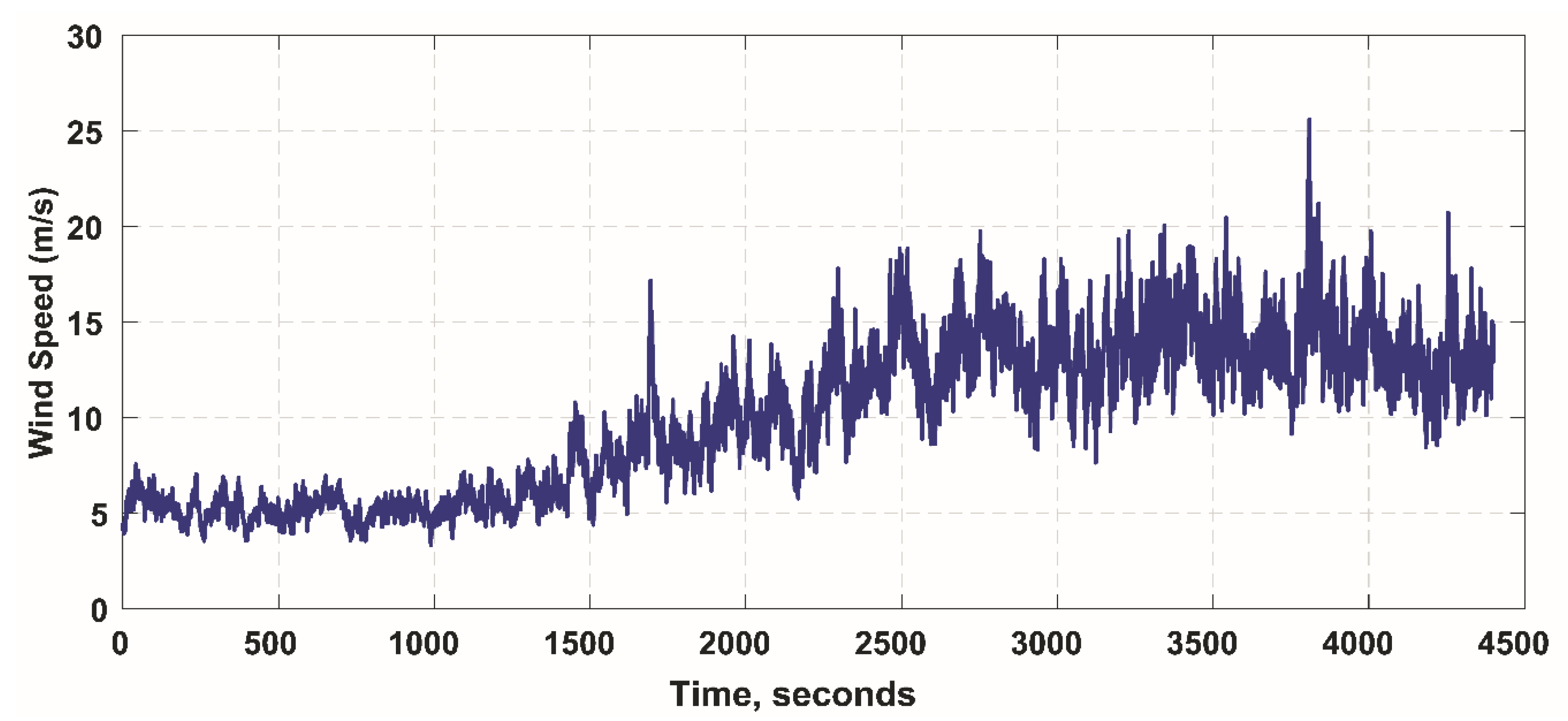
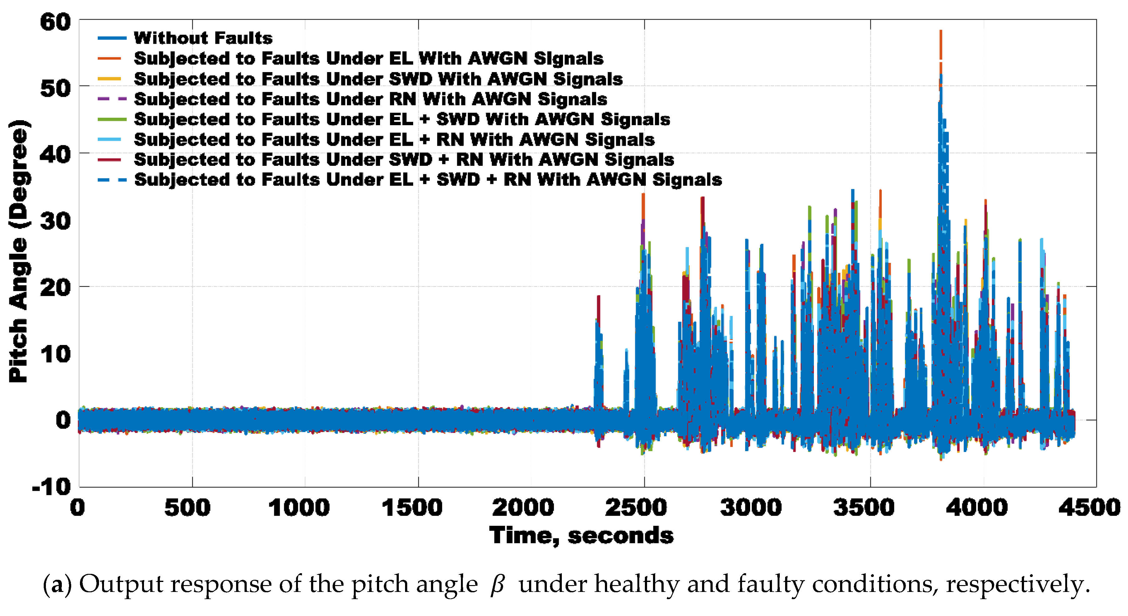
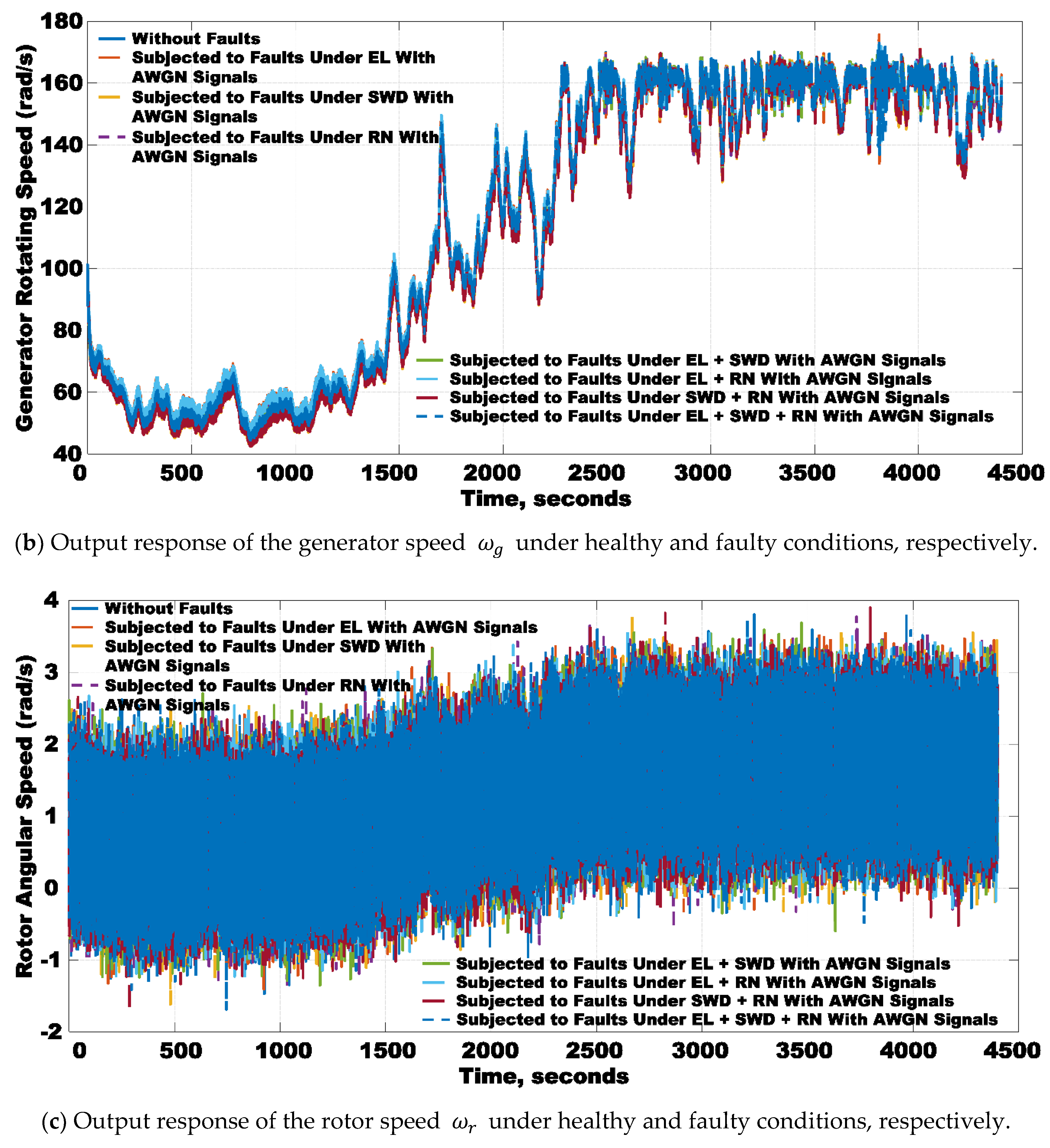
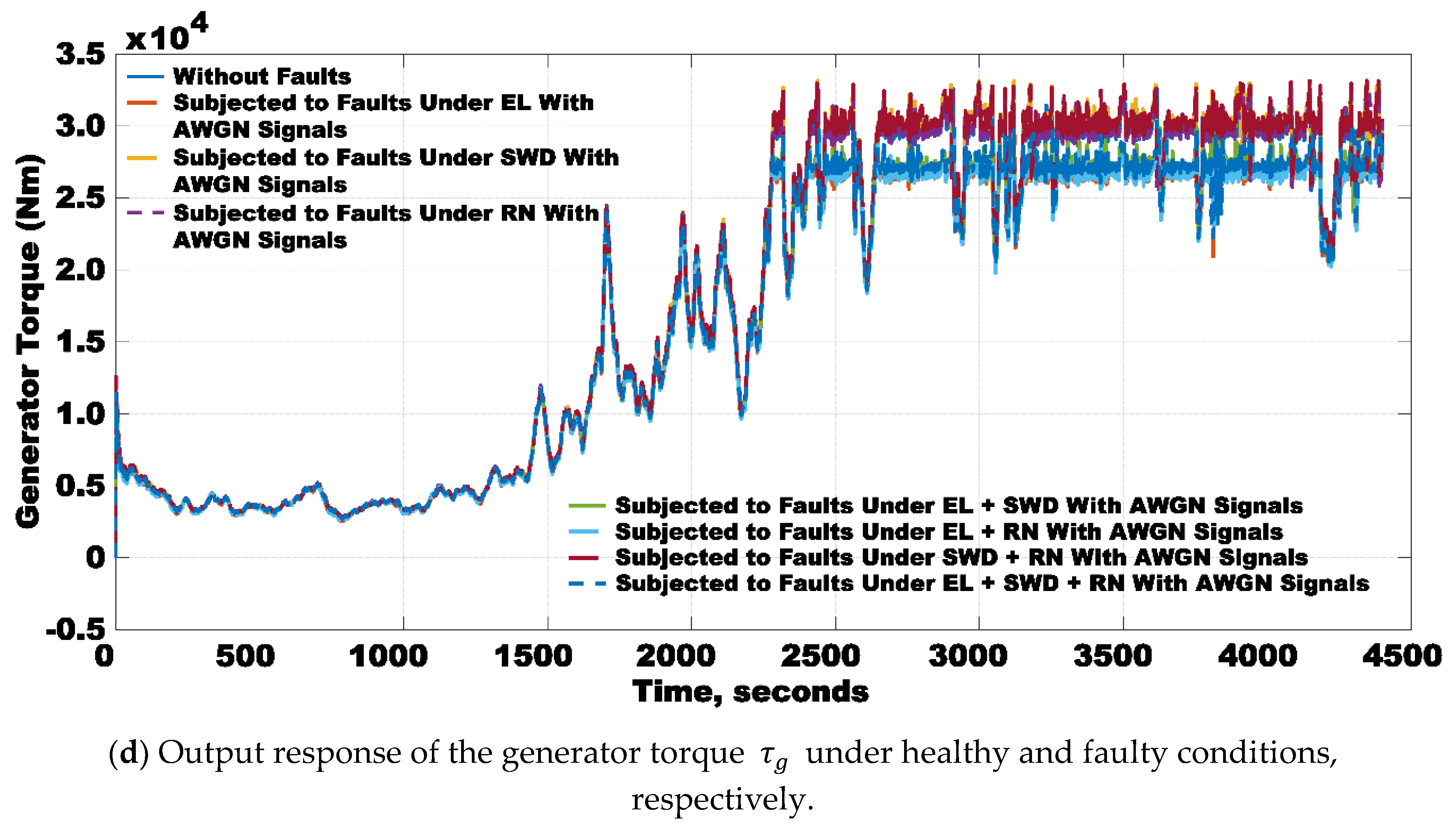
5.1. Time-Domain Space Characteristics of Wind Turbine Benchmark Systems

The curves displayed in Figure 9a–d show the time-domain responses of the four measurement outputs $\beta$, ${\omega }_g$, ${\omega }_r$, and ${\tau }_g$ under fault-free, and various faulty conditions of the actuator and sensor faults, including ‘EL’, ‘SWD’, ‘RN’, ‘EL + SWD’, ‘EL + RN’, ‘SWD + RN’, and ‘EL + SWD + RN’, respectively.

From Figure 9a–c, one can see that the curves are difficult to distinguish between fault-free and faulty situations. In Figure 9d, from 0–2300 s, it is impossible to find differences among the fault-free and faulty cases. From 2300–4400 s, one can see the fault-free curve is distinguishable from the faulty curves; however, it is hard to see the differences between the faulty curves. As a result, fault classification and diagnosis techniques are needed. It is noted that the overall simulated time of the 4.8 MW wind turbine benchmark system is 4400 s with the interval of 0.01 s. Consequently, the dimension of each experimental sample is 440,001.

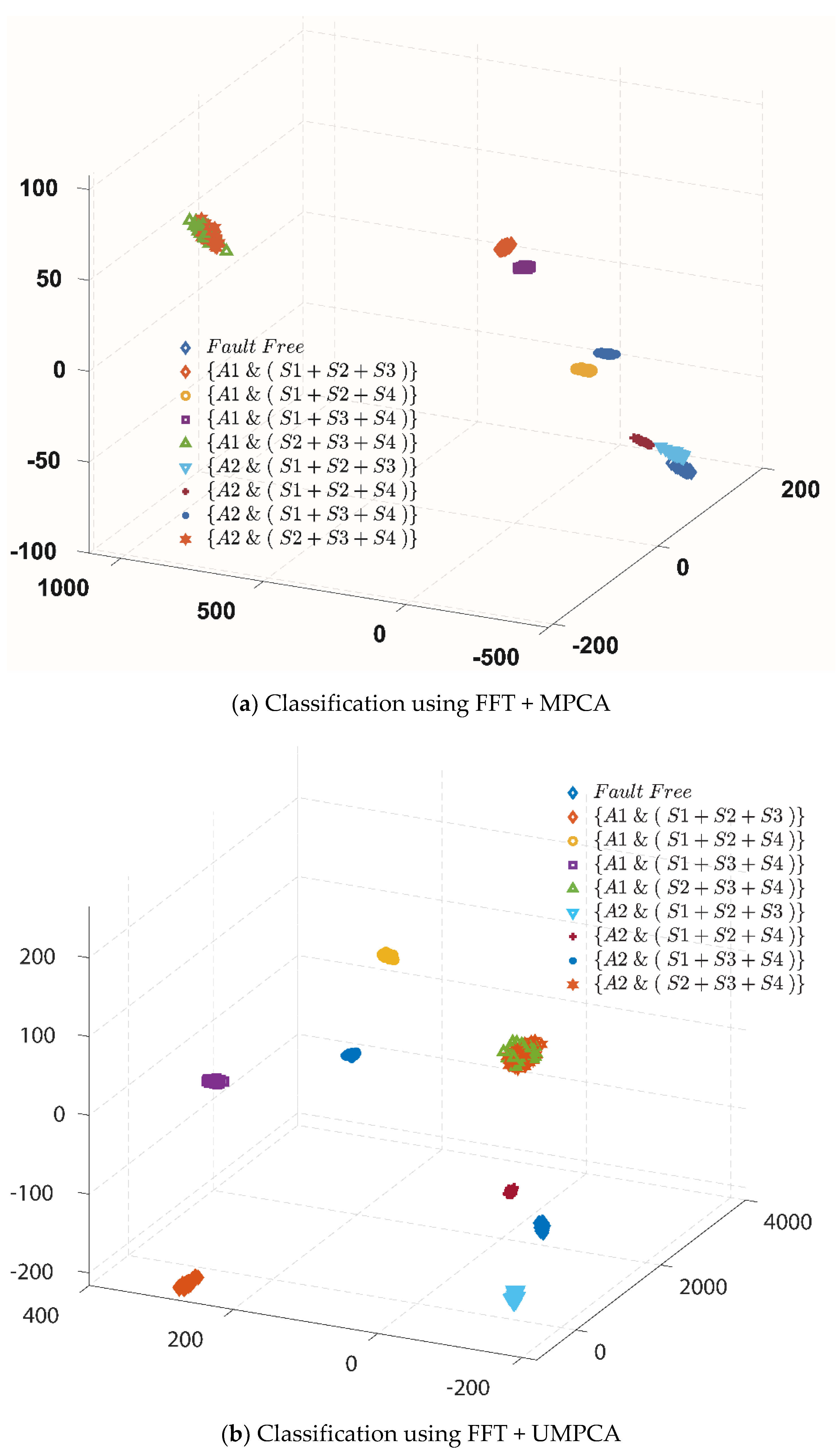
5.2. Feature Extractions and Fault Classifications for Scenario I

Data Set for Scenario I: In this data set, it includes ‘FF’ samples and eight types of ‘1AF + 3SFs’ samples. The detailed information is shown in Figure 6—Scenario I. In order to validate the effectiveness of the proposed algorithm by comparison, four types of tensor datasets are established, which are ${\mathit{X}}_{\mathrm{I}}^{MPCA}\in R^{\left\{440,000\times 4\times 9000\right\}}$, ${\mathit{X}}_{\mathrm{I}}^{UMPCA}\in R^{\left\{22,000\times 80\times 9000\right\}}$, ${\mathit{X}}_{\mathrm{I}}^{FFT+MPCA}\in R^{\left\{550\times 800\times 4\times 9000\right\}}$, and ${\mathit{X}}_{\mathrm{I}}^{FFT+UMPCA}\in R^{\left\{100\times 220\times 80\times 9000\right\}}$, respectively. The detailed information can be found in Table 5 and Table 6.

For ${\mathit{X}}_{\mathrm{I}}^{MPCA}\in R^{\left\{440,000\times 4\times 9000\right\}}$: ‘440,000’ represents the dimensionality of the feature subspace, ‘4’ stands for the dimensionality of the parameter subspace, and ‘9000’ illustrates the dimensionality of the sample subspace; for ${\mathit{X}}_{\mathrm{I}}^{UMPCA}\in R^{\left\{22,000\times 80\times 9000\right\}}$: ‘22,000’ represents the dimensionality of the feature subspace, ‘80’ stands for the dimensionality of the parameter subspace, and ‘9000’ illustrates the dimensionality of the sample subspace.

For ${\mathit{X}}_{\mathrm{I}}^{FFT+MPCA}\in R^{\left\{550\times 800\times 4\times 9000\right\}}$: The original data set ${\mathit{X}}_{\mathrm{I}}\in R^{\left\{440,000\times 36,000\right\}}$ is projected into a frequency-domain subspace and reshaped into a tensor data representation ${\mathit{X}}_{\mathrm{I}}^{FFT+MPCA}\in R^{\left\{550\times 800\times 4\times 9000\right\}}$ for the FFT + MPCA algorithm, where ‘4’ stands for the dimensionality of the parameter subspace, ‘9000’ illustrates the dimensionality of the sample subspace, and ‘500 × 800’ is the size of the reshaped feature matrix. For ${\mathit{X}}_{\mathrm{I}}^{FFT+UMPCA}\in R^{\left\{100\times 220\times 80\times 9000\right\}}$: The original data set ${\mathit{X}}_{\mathrm{I}}\in R^{\left\{440,000\times 36,000\right\}}$ is projected into a frequency-domain subspace and reshaped into a tensor dataset ${\mathit{X}}_{\mathrm{I}}^{FFT+UMPCA}\in R^{\left\{100\times 220\times 80\times 9000\right\}}$ for the FFT + UMPCA algorithm.

Fault classification under scenario I is shown by Figure 10 and Figure 11. Comparing Figure 10 with Figure 11, one can see that the three-dimensional space visualization results in Figure 11 are better than those in Figure 10. One can see, in Figure 11, that only two types of faulty condition cannot be distinguished, which are ‘{A1 & (S2 + S3 + S4)}’ and ‘{A2 & (S2 + S3 + S4)}’, respectively.

Specifically, from Figure 10a, the data generally cluster in three large groups, by using the MPCA algorithm, indicating a poor classification performance. To see the details, one can see one of the overlapping occurs between ‘Fault Free’ and ‘{A1 & (S1 + S3 + S4)}’, and the other exists between ‘{A1 & (S2 + S3 + S4)}’ and ‘{A2 & (S2 + S3 + S4)}’. Moreover, the rest of the five classes of faulty situations indistinguishably cluster together. From Figure 10b based on the UMPCA, the visualized results cluster around more groups, but are still unsatisfactory for classification.

From Figure 11a,b, one can see that both methods, that is, FFT + MPCA and FFT + UMPCA, can successfully classify seven classes of faulty/heathy conditions. It is noticed that the spatial distance amongst these generated features in Figure 11a is closer than that in Figure 11b in the corresponding three-dimensional space. In other words, there are larger distances between different faulty data in Figure 11b comparing with Figure 11a, indicating a better classification performance of the FFT + UMPCA algorithm. As a result, it is evident that the proposed FFT + UMPCA algorithm outperforms the MPCA, UMPCA, and FFT + MPCA for fault classification under scenario I.

5.3. Feature Extractions and Fault Classifications Based under Scenario II

Data Set for Scenario II: In this data set, it is composed of ‘FF’ samples and two types of ‘1AF + 4SFs’ samples. The detailed information is shown in Figure 6—Scenario II. In order to evaluate the effectiveness of the proposed algorithm by comparison, four types of datasets are constructed, which is ${\mathit{X}}_{\mathrm{II}}^{MPCA}\in R^{\left\{440,000\times 4\times 3000\right\}}$, ${\mathit{X}}_{\mathrm{II}}^{UMPCA}\in R^{\left\{22,000\times 80\times 3000\right\}}$, ${\mathit{X}}_{\mathrm{II}}^{FFT+MPCA}\in R^{\left\{550\times 800\times 4\times 3000\right\}}$, and ${\mathit{X}}_{\mathrm{II}}^{FFT+UMPCA}\in R^{\left\{100\times 220\times 80\times 3000\right\}}$, respectively. All the detailed information can be found in Table 5 and Table 6.

For ${\mathit{X}}_{\mathrm{II}}^{MPCA}\in R^{\left\{440,000\times 4\times 3000\right\}}$: ‘440,000’ represents the dimensionality of the feature subspace, ‘4’ stands for the dimensionality of parameter subspace, and ‘3000’ illustrates the dimensionality of the sample subspace. For ${\mathit{X}}_{\mathrm{II}}^{UMPCA}\in R^{\left\{22,000\times 80\times 3000\right\}}$: ‘22,000’ represents the dimensionality of the feature subspace, ‘80’ stands for the dimensionality of the parameter subspace, and ‘3000’ illustrates the dimensionality of the sample subspace.

For ${\mathit{X}}_{\mathrm{II}}^{FFT+MPCA}\in R^{\left\{550\times 800\times 4\times 3000\right\}}$: The original data set ${\mathit{X}}_{\mathrm{II}}\in R^{\left\{440,000\times 12,000\right\}}$ is projected into a frequency-domain subspace and reshaped into a tensor dataset ${\mathit{X}}_{\mathrm{II}}^{FFT+MPCA}\in R^{\left\{550\times 800\times 4\times 3000\right\}}$ for the FFT + MPCA algorithm. For ${\mathit{X}}_{\mathrm{II}}^{FFT+UMPCA}\in R^{\left\{100\times 220\times 80\times 3000\right\}}$: The original data set ${\mathit{X}}_{\mathrm{II}}\in R^{\left\{440,000\times 12,000\right\}}$ is projected into a frequency-domain subspace and reshaped into a tensor dataset ${\mathit{X}}_{\mathrm{II}}^{FFT+UMPCA}\in R^{\left\{100\times 220\times 80\times 3000\right\}}$ for the FFT + UMPCA algorithm..

In this section, Figure 12 and Figure 13 illustrate the three-dimensional space visualization performance for fault classification for wind turbine systems subjected to an actuator fault and four sensors faults simultaneously under AWGN noises, respectively using MPCA, UMPCA, FFT + MPCA, and FFT + UMPCA. From the simulated result observation, all types of faulty condition can only be successfully classified by using the FFT + MPCA and FFT + UMPCA methodologies. Therefore, FFT has a positive impact on the improvement of the performance of the dimensionality reduction and feature extraction.

Specifically, from Figure 12a,b, the data sets cluster in a distributive way, although the UMPCA performs a bit better in classification. Encouragingly, from Figure 13a,b, the data sets cluster in three clear groups, indicating a clear fault classification and diagnosis for the three faulty/healthy conditions concerned. From Figure 13b, it is interesting to observe the data in the same group shape distinguishably. It is noted that faulty data in this study includes seven types of faults, such as effectiveness loss, sinusoidal faults, and random number disturbances and so forth, and the fault-free data are subjected to stochastic noises. Therefore, the classification by using the FFT + MPCA can recognize the difference between the data in the same large group. In other words, Figure 13b can also reflect the intrinsic properties of the original samples of the 4.8 MW wind turbine benchmark system.

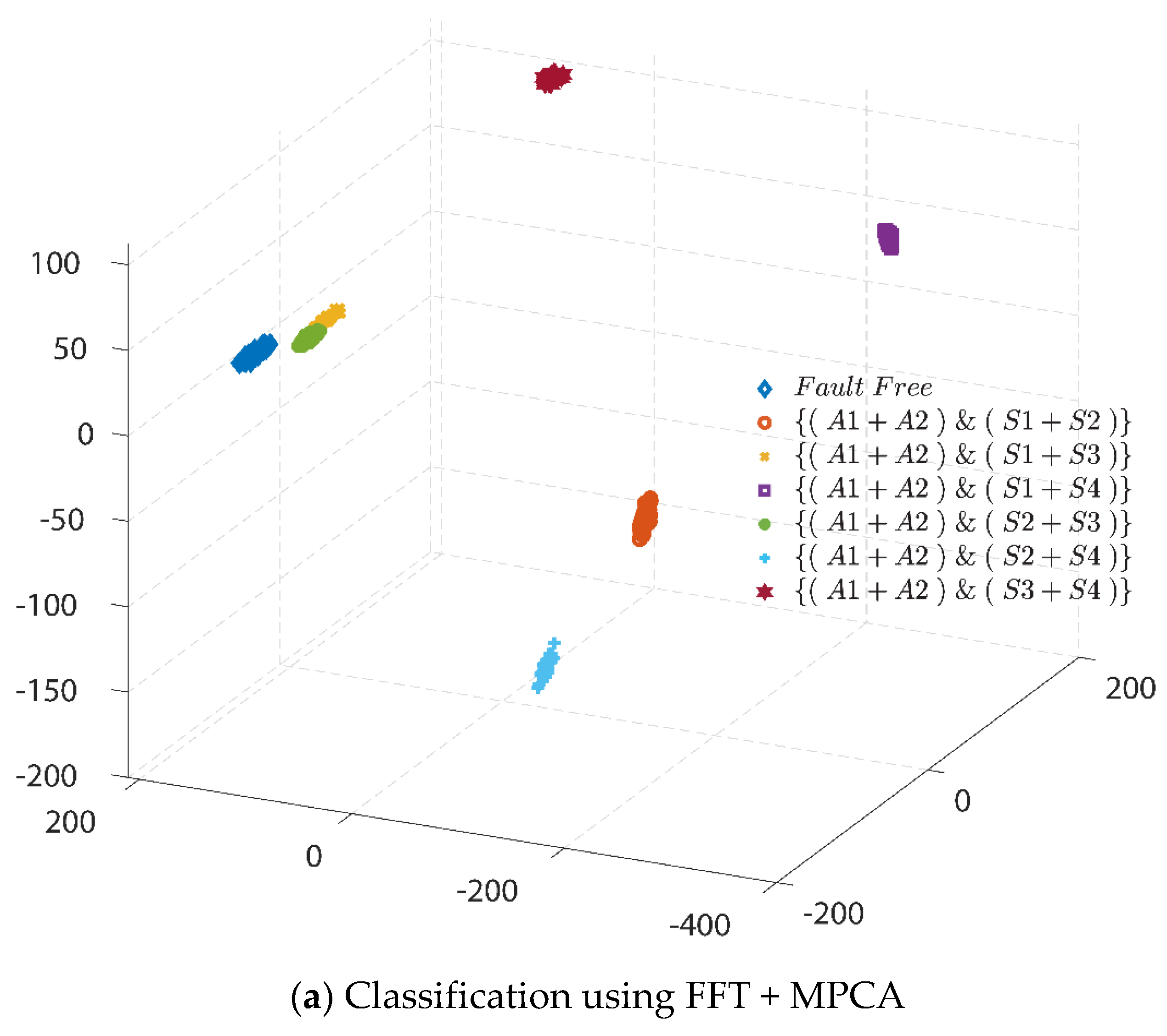
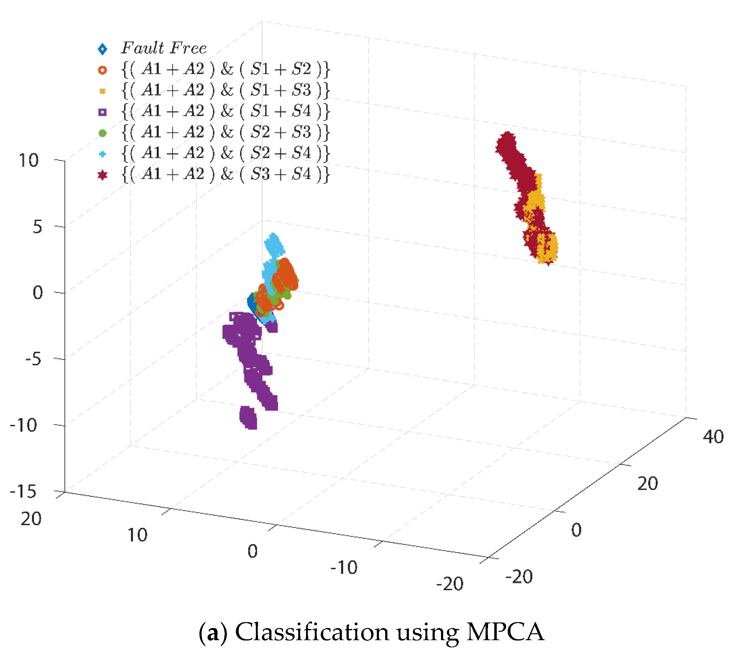
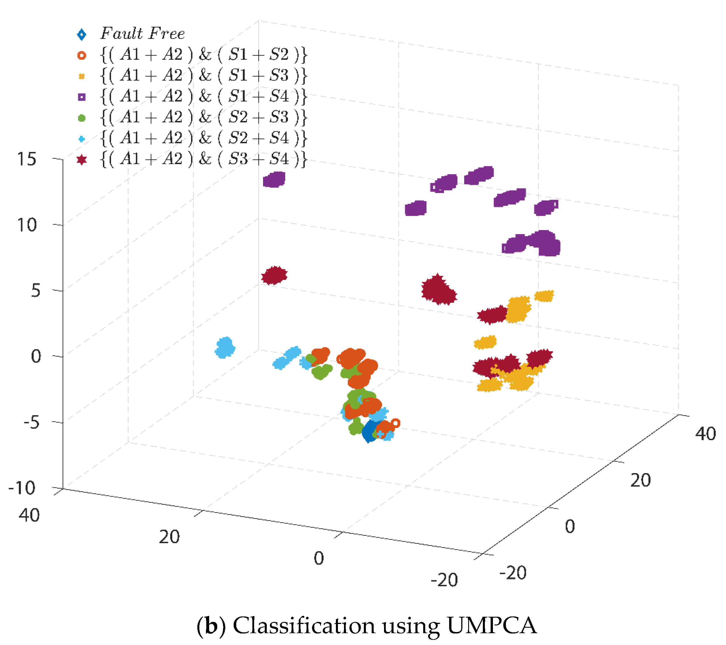
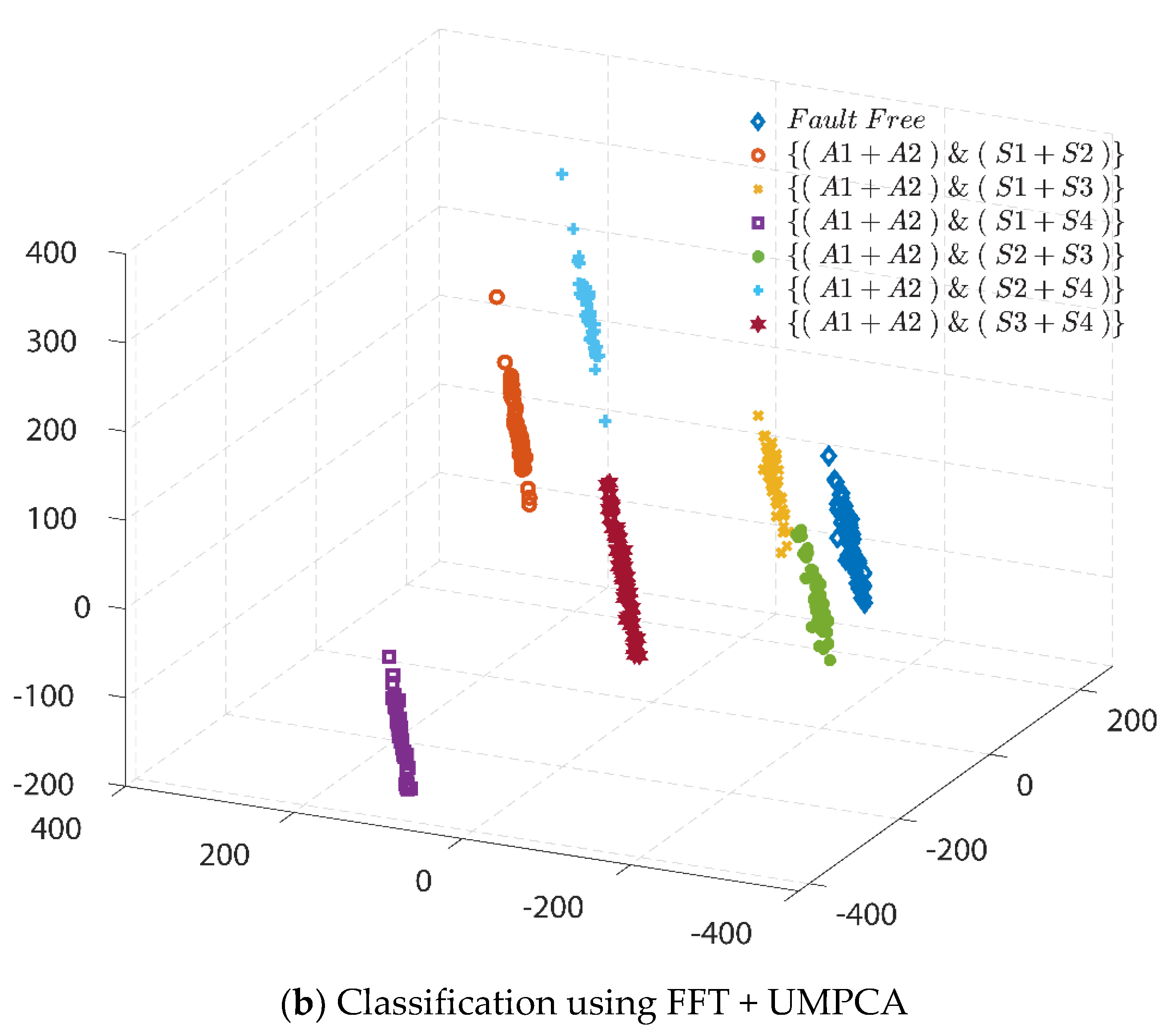
5.4. Feature Extractions and Fault Classifications under Scenario III

Data Set for Scenario III: In this data set, it includes ‘FF’ samples and six types of ‘2AFs + 2SFs’ samples. The detailed information is shown in Figure 7—Scenario III. In order to validate the effectiveness of the proposed algorithm by comparison, four types of datasets are addressed, which is ${\mathit{X}}_{\mathrm{III}}^{MPCA}\in R^{\left\{440,000\times 4\times 7000\right\}}$, ${\mathit{X}}_{\mathrm{III}}^{UMPCA}\in R^{\left\{22,000\times 80\times 7000\right\}}$, ${\mathit{X}}_{\mathrm{III}}^{FFT+MPCA}\in R^{\left\{550\times 800\times 4\times 7000\right\}}$, and ${\mathit{X}}_{\mathrm{III}}^{FFT+UMPCA}\in R^{\left\{100\times 220\times 80\times 7000\right\}}$, respectively. All the detailed information can be found in Table 5 and Table 6.

For ${\mathit{X}}_{\mathrm{III}}^{MPCA}\in R^{\left\{440,000\times 4\times 7000\right\}}$: ‘440,000’ represents the dimensionality of the feature subspace, ‘4’ stands for the dimensionality of the parameter subspace, and ‘7000’ illustrates the dimensionality of the sample subspace. For ${\mathit{X}}_{\mathrm{III}}^{UMPCA}\in R^{\left\{22,000\times 80\times 7000\right\}}$: ‘22,000’ represents the dimensionality of the feature subspace, ‘80’ stands for the dimensionality of parameter subspace, and ‘7000’ illustrates the dimensionality of the sample subspace.

For ${\mathit{X}}_{\mathrm{III}}^{FFT+MPCA}\in R^{\left\{550\times 800\times 4\times 7000\right\}}$: The original data set ${\mathit{X}}_{\mathrm{III}}\in R^{\left\{440,000\times 28,000\right\}}$ is projected into a frequency-domain subspace and reshaped into a tensor dataset ${\mathit{X}}_{\mathrm{III}}^{FFT+MPCA}\in R^{\left\{550\times 800\times 4\times 7000\right\}}$ for using the FFT + MPCA algorithm. For ${\mathit{X}}_{\mathrm{III}}^{FFT+UMPCA}\in R^{\left\{100\times 220\times 80\times 7000\right\}}$: The original data set ${\mathit{X}}_{\mathrm{III}}\in R^{\left\{440,000\times 28,000\right\}}$ is projected into a frequency-domain subspace and reshaped into a tensor dataset ${\mathit{X}}_{\mathrm{III}}^{FFT+UMPCA}\in R^{\left\{100\times 220\times 80\times 7000\right\}}$ for the FFT + UMPCA algorithm.

In this section, Figure 14 and Figure 15 exhibit the three-dimensional space visualization performance for fault classification for wind turbine systems subjected to two actuator faults and two sensor faults simultaneously under AWGN noise corruption, respectively by using MPCA, UMPCA, FFT + MPCA, and FFT + UMPCA.

From Figure 14a, it is shown that two large groups are formed in the corresponding three-dimensional space based on the MPCA method. It is observed that the overlapping occurs between ‘{(A1 + A2) & (S1 + S3)}’ and ‘{(A1 + A2) & (S3 + S4)}’, and another overlapping happens among ‘Fault Free’, ‘{(A1 + A2) & (S1 + S2)}’, ‘{(A1 + A2) & (S1 + S4)}’, ‘{(A1 + A2) & (S2 + S3)}’, and ‘{(A1 + A2) & (S2 + S4)}’. From Figure 14b based on the UMPCA technique, the visualization performance, with more formed data groups, is slightly better than that using the MPCA but is far from acceptable for classification.

Seven classes of faulty/healthy situations were successfully classified respectively by using the FFT + MPCA shown in Figure 15a and FFT + UMPCA exhibited by Figure 15b. More interesting, Figure 15b can clearly reflect the intrinsic properties of the original samples of the wind turbines, which indicates the FFT + UMPCA approach can also sense different types of faults in every single faulty situation.

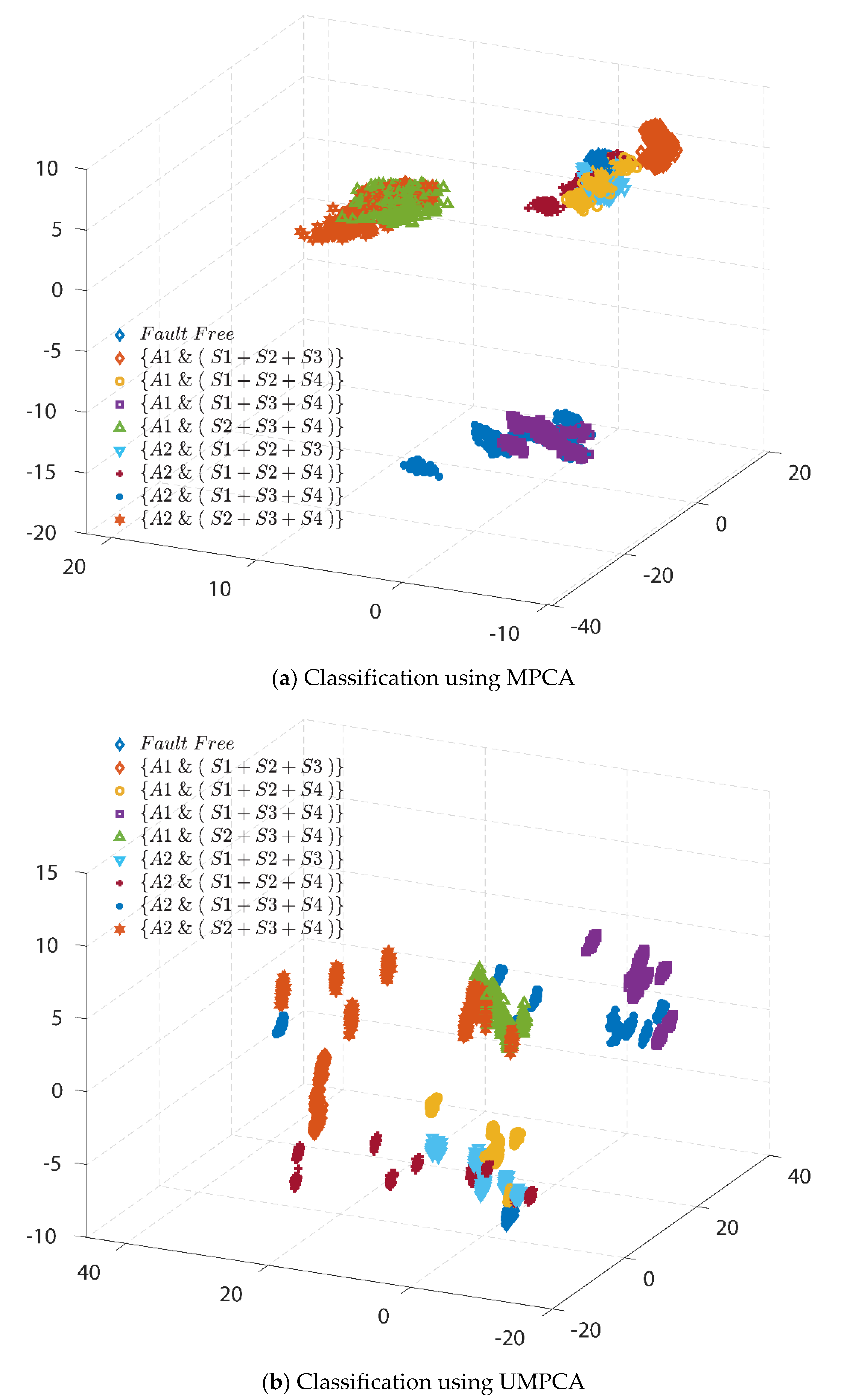
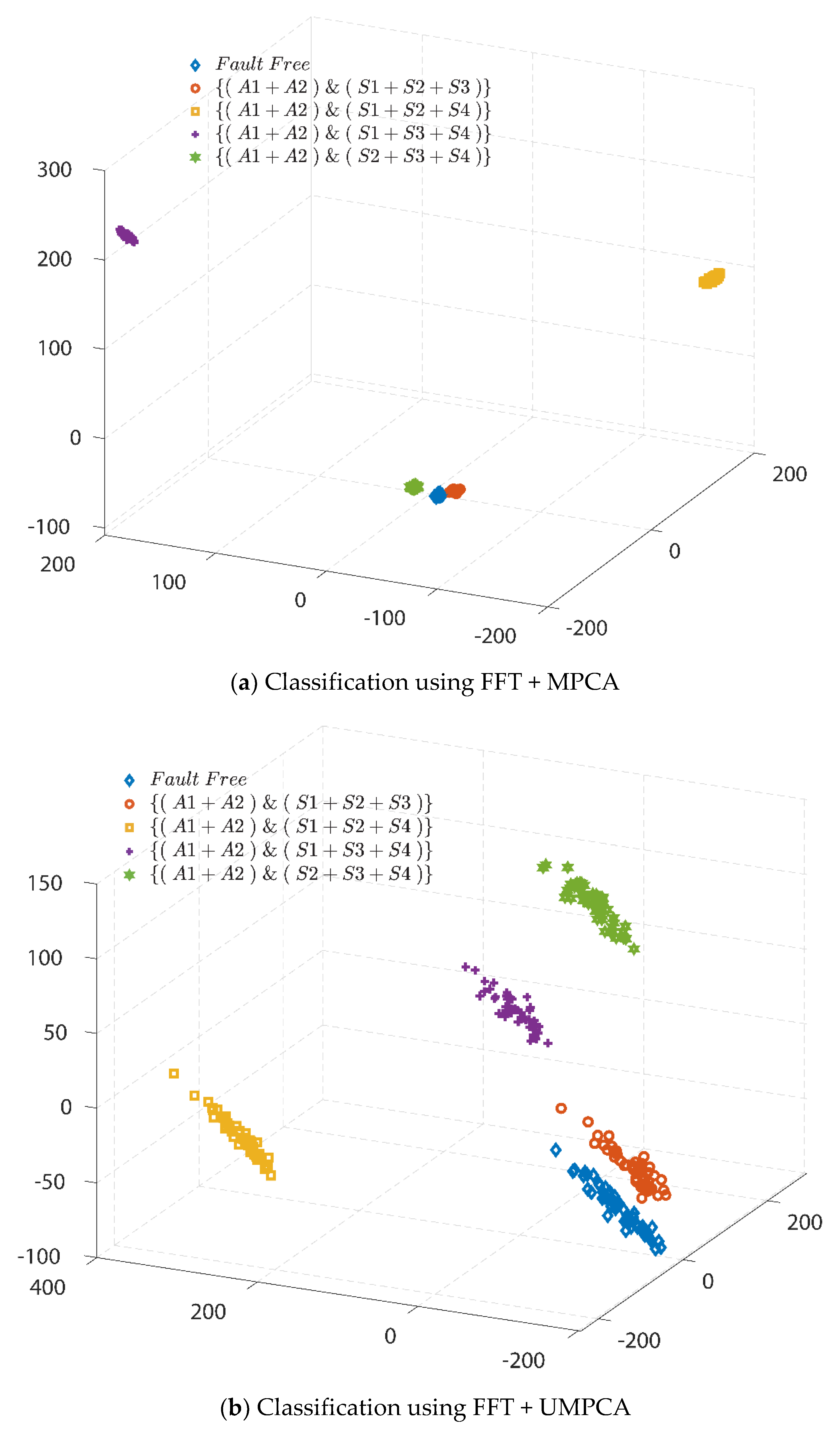
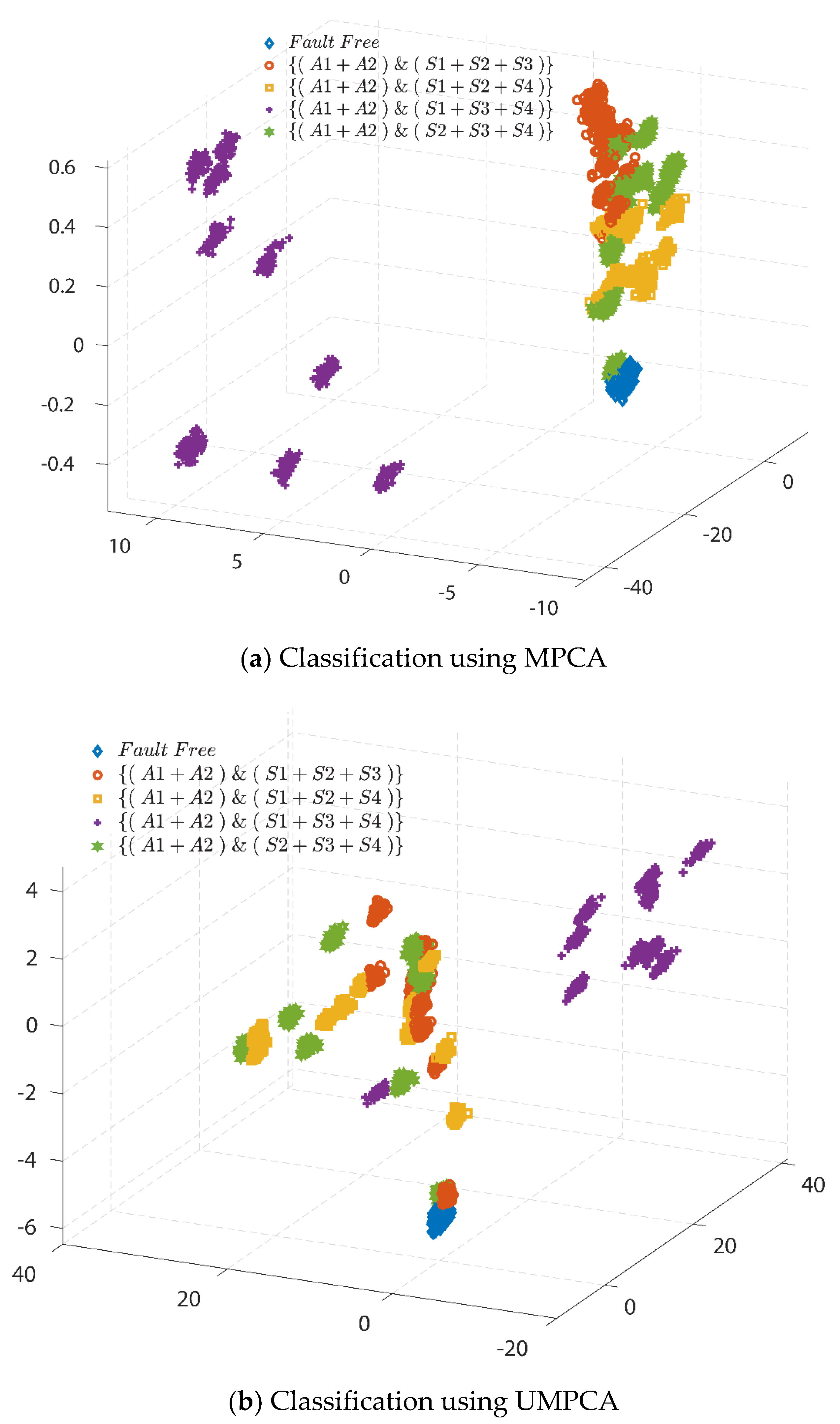
5.5. Feature Extractions and Fault Classifications Based under Scenario IV

Data Set for Scenario IV: In this data set, it consists in ‘FF’ samples and four types of ‘2AFs + 3SFs’ samples. The detailed information is shown in Figure 8—Scenario IV. In order to evaluate the effectiveness of the proposed algorithm by comparison, four types of datasets are determined: ${\mathit{X}}_{\mathrm{IV}}^{MPCA}\in R^{\left\{440,000\times 4\times 5000\right\}}$, ${\mathit{X}}_{\mathrm{IV}}^{UMPCA}\in R^{\left\{22,000\times 80\times 5000\right\}}$, ${\mathit{X}}_{\mathrm{IV}}^{FFT+MPCA}\in R^{\left\{550\times 800\times 4\times 5000\right\}}$, and ${\mathit{X}}_{\mathrm{IV}}^{FFT+UMPCA}\in R^{\left\{100\times 220\times 80\times 5000\right\}}$, respectively. All the detailed information can be found in Table 5 and Table 6.

For ${\mathit{X}}_{\mathrm{IV}}^{MPCA}\in R^{\left\{440,000\times 4\times 5000\right\}}$: ‘440,000’ represents the dimensionality of the feature subspace, ‘4’ stands for the dimensionality of the parameter subspace, and ‘5000’ illustrates the dimensionality of the sample subspace. For ${\mathit{X}}_{\mathrm{IV}}^{UMPCA}\in R^{\left\{22,000\times 80\times 5000\right\}}$: ‘22,000’ represents the dimensionality of the feature subspace, ‘80’ stands for the dimensionality of the parameter subspace, and ‘5000’ illustrates the dimensionality of the sample subspace.

For ${\mathit{X}}_{\mathrm{IV}}^{FFT+MPCA}\in R^{\left\{550\times 800\times 4\times 5000\right\}}$: The original data set ${\mathit{X}}_{\mathrm{IV}}\in R^{\left\{440,000\times 20,000\right\}}$ is projected into a frequency-domain subspace and reshaped into a tensor representation ${\mathit{X}}_{\mathrm{IV}}^{FFT+MPCA}\in R^{\left\{550\times 800\times 4\times 5000\right\}}$ for the use of the FFT + MPCA algorithm. For ${\mathit{X}}_{\mathrm{IV}}^{FFT+UMPCA}\in R^{\left\{100\times 220\times 80\times 5000\right\}}$: The original data set ${\mathit{X}}_{\mathrm{IV}}\in R^{\left\{440,000\times 20,000\right\}}$ is projected into a frequency-domain subspace and reshaped into a tensor representation ${\mathit{X}}_{\mathrm{IV}}^{FFT+UMPCA}\in R^{\left\{100\times 220\times 80\times 5000\right\}}$ for the implementation of the FFT + UMPCA technique.

In this subsection, Figure 16 and Figure 17 exhibit the three-dimensional space visualization performance for fault classification for wind turbine systems subjected to two simultaneous actuator faults and three simultaneous sensors under AWGN noise corruptions, by using the MPCA, UMPCA, FFT + MPCA, and FFT + UMPCA algorithms, respectively.

From Figure 16a based on the MPCA, the data are clustering around three large sets, while in Figure 16b using the UMPCA, the data are clustering in a more distributed way. Both of the visualized results in Figure 16a,b fail to classify and diagnose the faults.

From Figure 17a,b, faulty conditions can be successfully classified by both FFT + MPCA and FFT + UMPCA algorithms. Specifically, it is worthy to point out that the corresponding three-dimensional space visualization behaviours in Figure 17a,b shape differently in comparison with Figure 16a,b, respectively. From what is exhibited in Figure 17a, one can see that the FFT + MPCA methods outperform the MPCA. The reason behind this is that the intrinsic structures of the obtained experimental data sets were reconstructed by using Fourier transform bases. Additionally, these samples are mapped into the multi-dimensional frequency-domain subspace, which means the visualized performance/behaviour are different from the MPCA-based circumstances. Furthermore, the performance of the FFT + UMPCA in Figure 17b is much better than that based on the UMPCA in Figure 16b. Consequently, the FFT has a positive impact on the improvement of the performance of the fault classification and diagnosis. From Figure 17b, one can see that the FFT + UMPCA approach can also recognize the differences of data in the same group.

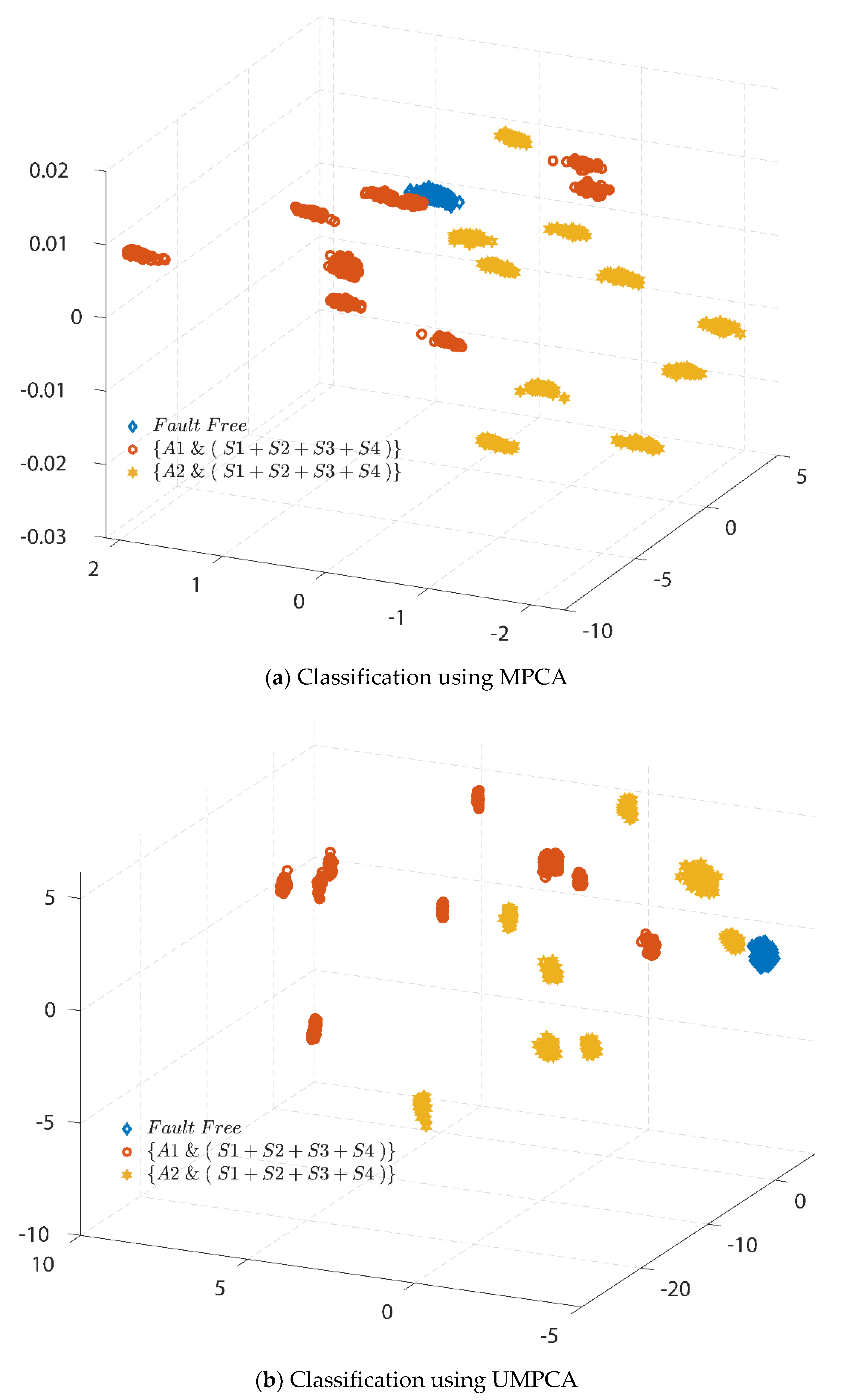
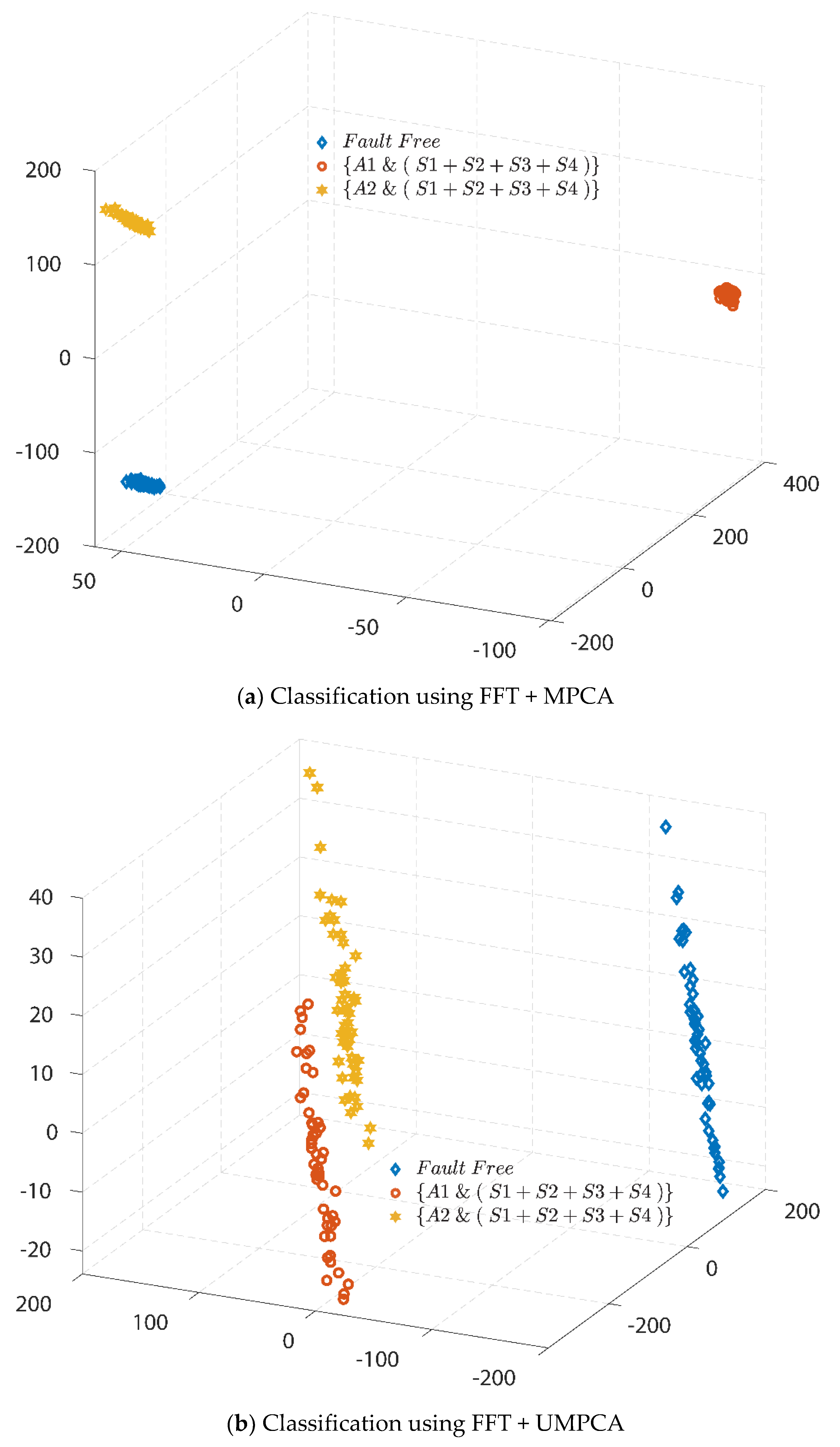
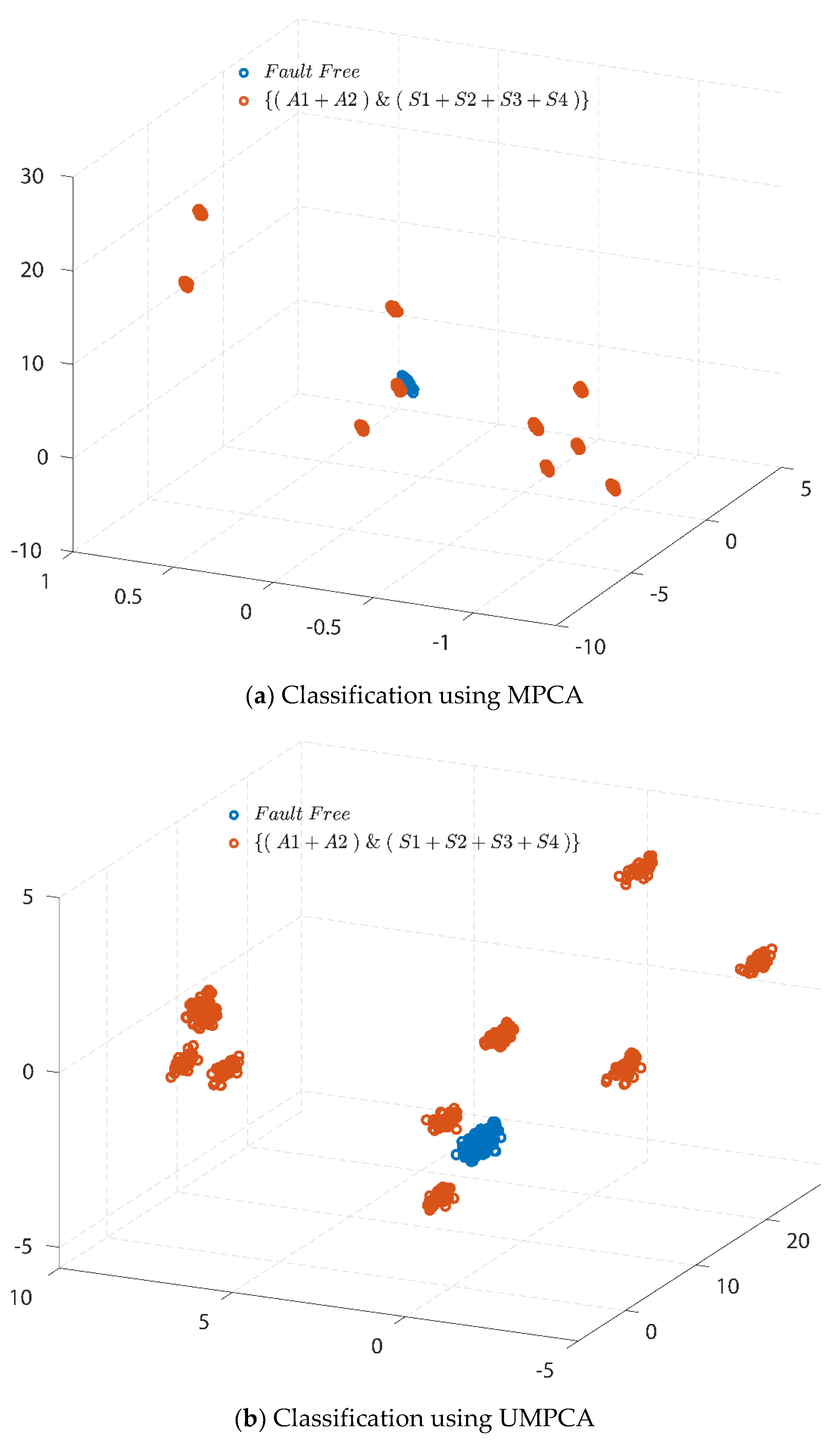
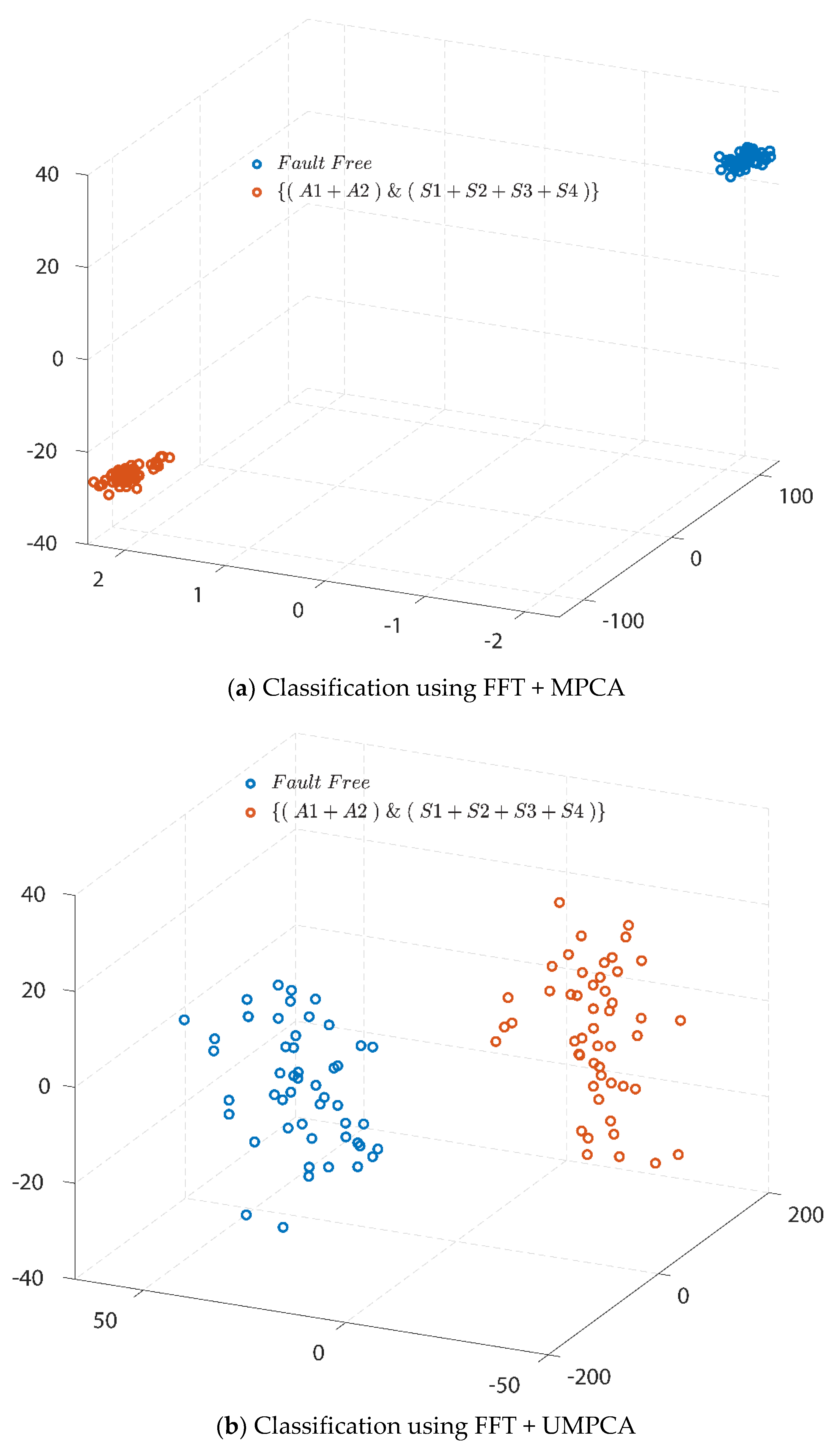
5.6. Feature Extractions and Fault Classifications Based under Scenario V

Data Set for Scenario V: In this data set, it is combined by ‘FF’ and ‘2AFs + 4SFs’ samples. The detailed information is shown in Figure 8—Scenario V. In order to validate the effectiveness of the proposed algorithm by comparison, four types of datasets are built: ${\mathit{X}}_{\mathrm{V}}^{MPCA}\in R^{\left\{440,000\times 4\times 2000\right\}}$, ${\mathit{X}}_{\mathrm{V}}^{UMPCA}\in R^{\left\{22,000\times 80\times 2000\right\}}$, ${\mathit{X}}_{\mathrm{V}}^{FFT+MPCA}\in R^{\left\{550\times 800\times 4\times 2000\right\}}$, and ${\mathit{X}}_{\mathrm{V}}^{FFT+UMPCA}\in R^{\left\{100\times 220\times 80\times 2000\right\}}$, respectively. All the detailed information can be found in Table 5 and Table 6.

For ${\mathit{X}}_{\mathrm{V}}^{MPCA}\in R^{\left\{440,000\times 4\times 2000\right\}}$: ‘440,000’ represents the dimensionality of the feature subspace, ‘4’ stands for the dimensionality of the parameter subspace, and ‘2000’ indicates the dimensionality of the sample subspace. For ${\mathit{X}}_{\mathrm{V}}^{UMPCA}\in R^{\left\{22,000\times 80\times 2000\right\}}$: ‘22,000’ represents the dimensionality of the feature subspace, ‘80’ stands for the dimensionality of the parameter subspace, and ‘2000’ represents the dimensionality of the sample subspace.

For ${\mathit{X}}_{\mathrm{V}}^{FFT+MPCA}\in R^{\left\{550\times 800\times 4\times 2000\right\}}$: The original data set ${\mathit{X}}_{\mathrm{V}}\in R^{\left\{440,000\times 8000\right\}}$ is projected into a frequency-domain subspace and reshaped into a tensor dataset ${\mathit{X}}_{\mathrm{V}}^{FFT+MPCA}\in R^{\left\{550\times 800\times 4\times 2000\right\}}$ for the use of the FFT + MPCA algorithm. The original data set ${\mathit{X}}_{\mathrm{V}}\in R^{\left\{440,000\times 8000\right\}}$ is projected into a frequency-domain subspace and reshaped into a tensor representation ${\mathit{X}}_{\mathrm{V}}^{FFT+UMPCA}\in R^{\left\{100\times 220\times 80\times 2000\right\}}$ for the FFT + UMPCA technique.

Figure 18 and Figure 19 show the three-dimensional space visualization performance for fault classification for wind turbine systems subjected to two simultaneous actuators faults and four simultaneous sensors faults corrupted by AWGN noisy signals, respectively using different algorithms, such as MPCA, UMPCA, FFT + MPCA, and FFT + UMPCA.

From Figure 18a based on the MPCA, the faulty-data cluster in 10 groups, and one of them is overlapped with the fault-free data, indicating unsuccessful fault classification. From Figure 18b based on the UMPCA technique, the visualization performance is relatively better than that using the MPCA, as there is no overlapping between the faulty-data and fault-free data. However, the performance in Figure 18b is still not satisfactory, since the distances between the faulty-data are too large and the distances between the fault-free data and some of the faulty-data are quite close.

From Figure 19a, one can see that FFT + MPCA method has a much better classification performance than the MPCA, shown in Figure 18a, as the faulty data and fault-free data are clearly classified into two separated groups by using FFT + MPCA. Comparing Figure 19b by using FFT + UMPCA to Figure 18b via the UMPCA, the faulty data and fault-free data are separated into two large groups in Figure 19b, showing a clear classification between the faulty data and fault free data. As a result, it is evident that the FFT has a positive impact on the improvement of the performance of the fault classification and diagnosis. In addition, from Figure 19b, the data in the same group are not clustered so close compared with Figure 19a. As the faulty data is a combination of the data subjected to different types, such as effectiveness loss, sinusoidal fault signal, random number disturbances, and so forth, this means the FFT + UMPCA can sense the difference between these data.

It is noted that the MPCA approach determines a tensor-to-tensor projection that captures most of the signal variation present in the original tensor representation, whereas, the UMPCA method uses the tensor-to-vector projection. For the MPCA technique, some of the correlations of the principal components among the projected directions are neglected to some extent. Compared with MPCA, UMPCA can exclude the possibilities of getting significant features with similar geometric structures, depending on the methodology of tensor-to-vector projection. The reason behind is that the UMPCA algorithm concentrates on extracting and determining the uncorrelated principal components rather than the conventional principal components in the MPCA technique. Moreover, the FFT preprocessing technique can enhance the data classification capability of the UMPCA. As a result, this is why the proposed FFT + UMPCA can effectively classify the fault under all five scenarios above.

6. Conclusions

In this paper, fast Fourier transform (FFT) and uncorrelated multi-linear principal component analysis (UMPCA) techniques were integrated for fault classification of the 4.8 MW benchmark wind turbine systems subjected to multiple actuator and sensor faults under five scenarios of actuator and sensor faults. The detailed comparison studies were carried out, and the effectiveness of the proposed algorithm was well demonstrated. It is worthy to point out, among all the used algorithms, the FFT has a positive impact on the improvement of the performance of the fault diagnosis and classification. The proposed FFT plus UMPCA algorithm can not only classify the various classes of faulty conditions but can also recognize the differences between the data within the same class.

In the future, it is of interest to investigate data-driven fault prognosis and remaining useful life prediction for wind turbine systems. It is also promising to enhance fault diagnosis and prognosis performance by using hybrid methods (by integrating various data-driven fault diagnosis/prognosis methods or even by combining model-based approaches and data-driven based methods).

References

1. Rashid, M.H. Electric Renewable Energy Systems; Elsevier, Academic Press: San Diego, CA, USA, 2016. [Google Scholar]
2. Gao, R.; Gao, Z. Pitch control for wind turbine systems using optimization, estimation and compensation. Renew. Energy 2016, 91, 501–515. [Google Scholar] [CrossRef]
3. Wind Europe. Wind Energy in Europe in 2019: Trends and Statistics. 2020. Available online: https://windeurope.org/wp-content/uploads/files/about-wind/statistics/WindEurope-Annual-Statistics-2019.pdf (accessed on 10 August 2020).
4. Gao, Z.; Sheng, S. Real-time monitoring, prognosis, and resilient control for wind turbine systems. Renew. Energy 2018, 116, 1–4. [Google Scholar] [CrossRef]
5. Hameed, Z.; Hong, Y.; Cho, Y.; Ahn, S.-H.; Song, C. Condition monitoring and fault detection of wind turbines and related algorithms: A review. Renew. Sustain. Energy Rev. 2009, 13, 1–39. [Google Scholar] [CrossRef]
6. Márquez, F.; Tobias, A.M.; Pérez, J.M.P.; Papaelias, M. Condition monitoring of wind turbines: Techniques and methods. Renew. Energy 2012, 46, 169–178. [Google Scholar] [CrossRef]
7. Liu, X.; Gao, Z.; Chen, M.Z.Q. Takagi–Sugeno Fuzzy Model Based Fault Estimation and Signal Compensation with Application to Wind Turbines. IEEE Trans. Ind. Electron. 2017, 64, 5678–5689. [Google Scholar] [CrossRef]
8. Simani, S.; Farsoni, S.; Castaldi, P. Fault Diagnosis of a Wind Turbine Benchmark via Identified Fuzzy Models. IEEE Trans. Ind. Electron. 2014, 62, 3775–3782. [Google Scholar] [CrossRef]
9. Rahimilarki, R.; Gao, Z.; Zhang, A.; Binns, R. Robust Neural Network Fault Estimation Approach for Nonlinear Dynamic Systems with Applications to Wind Turbine Systems. IEEE Trans. Ind. Inform. 2019, 15, 6302–6312. [Google Scholar] [CrossRef]
10. Chen, J.; Patton, R.J. Robust Model-Based Fault Diagnosis for Dynamic Systems; Kluwer: Boston, MA, USA, 1999. [Google Scholar]
11. Venkatasubramanian, V.; Rengaswamy, R.; Yin, K.; Kavuri, S.N. A review of process fault detection and diagnosis. Comput. Chem. Eng. 2003, 27, 293–311. [Google Scholar] [CrossRef]
12. Gao, Z.; Cecati, C.; Ding, S.X. A Survey of Fault Diagnosis and Fault-Tolerant Techniques—Part I: Fault Diagnosis with Model-Based and Signal-Based Approaches. IEEE Trans. Ind. Electron. 2015, 62, 3757–3767. [Google Scholar] [CrossRef] [Green Version]
13. Gao, Z.; Cecati, C.; Ding, S.X. A Survey of Fault Diagnosis and Fault-Tolerant Techniques Part II: Fault Diagnosis with Knowledge-Based and Hybrid/Active Approaches. IEEE Trans. Ind. Electron. 2015, 62, 3768–3774. [Google Scholar] [CrossRef] [Green Version]
14. Gao, Z.; Ding, S.X.; Cecati, C. Real-time fault diagnosis and fault-tolerant control. IEEE Trans. Ind. Electron. 2015, 62, 3752–3756. [Google Scholar] [CrossRef] [Green Version]
15. Zhang, D.; Gao, Z. Improvement of Refrigeration Efficiency by Combining Reinforcement Learning with a Coarse Model. Processes 2019, 7, 967. [Google Scholar] [CrossRef] [Green Version]
16. Bergen, K.J.; Johnson, P.A.; De Hoop, M.V.; Beroza, G.C. Machine learning for data-driven discovery in solid Earth geoscience. Science 2019, 363, eaau0323. [Google Scholar] [CrossRef] [PubMed]
17. Oh, H.; Jung, J.H.; Jeon, B.C.; Youn, B.D. Scalable and Unsupervised Feature Engineering Using Vibration-Imaging and Deep Learning for Rotor System Diagnosis. IEEE Trans. Ind. Electron. 2018, 65, 3539–3549. [Google Scholar] [CrossRef]
18. Song, W.; Wen, L.; Gao, L.; Li, X. Unsupervised fault diagnosis method based on iterative multi-manifold spectral clustering. IET Collab. Intell. Manuf. 2019, 1, 48–55. [Google Scholar] [CrossRef]
19. Holtzman, B.K.; Paté, A.; Paisley, J.; Waldhauser, F.; Repetto, D. Machine learning reveals cyclic changes in seismic source spectra in Geysers geothermal field. Sci. Adv. 2018, 4, 5. [Google Scholar] [CrossRef] [Green Version]
20. Phan, H.T.H.; Kumar, A.; Feng, D.; Fulham, M.J.; Kim, J. Unsupervised Two-Path Neural Network for Cell Event Detection and Classification Using Spatiotemporal Patterns. IEEE Trans. Med. Imaging 2018, 38, 1477–1487. [Google Scholar] [CrossRef]
21. Zhao, R.; Wang, D.; Yan, R.; Mao, K.; Shen, F.; Wang, J. Machine Health Monitoring Using Local Feature-Based Gated Recurrent Unit Networks. IEEE Trans. Ind. Electron. 2018, 65, 1539–1548. [Google Scholar] [CrossRef]
22. Elforjani, M.; Shanbr, S. Prognosis of Bearing Acoustic Emission Signals Using Supervised Machine Learning. IEEE Trans. Ind. Electron. 2018, 65, 5864–5871. [Google Scholar] [CrossRef] [Green Version]
23. Adeli, E.; Thung, K.-H.; An, L.; Wu, G.; Shi, F.; Wang, P.; Shen, D. Semi-Supervised Discriminative Classification Robust to Sample-Outliers and Feature-Noises. IEEE Trans. Pattern Anal. Mach. Intell. 2019, 41, 515–522. [Google Scholar] [CrossRef]
24. Razavi-Far, R.; Hallaji, E.; Farajzadeh-Zanjani, M.; Saif, M.; Kia, S.H.; Henao, H.; Capolino, G.-A. Information Fusion and Semi-Supervised Deep Learning Scheme for Diagnosing Gear Faults in Induction Machine Systems. IEEE Trans. Ind. Electron. 2019, 66, 6331–6342. [Google Scholar] [CrossRef]
25. Zhao, M.; Kang, M.; Tang, B.; Pecht, M. Multiple Wavelet Coefficients Fusion in Deep Residual Networks for Fault Diagnosis. IEEE Trans. Ind. Electron. 2019, 66, 4696–4706. [Google Scholar] [CrossRef]
26. Ge, Z.; Song, Z.; Ding, S.X.; Huang, B. Data Mining and Analytics in the Process Industry: The Role of Machine Learning. IEEE Access 2017, 5, 20590–20616. [Google Scholar] [CrossRef]
27. Guo, M.-F.; Yang, N.-C.; Chen, W.-F. Deep-Learning-Based Fault Classification Using Hilbert–Huang Transform and Convolutional Neural Network in Power Distribution Systems. IEEE Sens. J. 2019, 19, 6905–6913. [Google Scholar] [CrossRef]
28. Pan, T.; Chen, J.; Zhou, Z.; Wang, C.; He, S. A Novel Deep Learning Network via Multiscale Inner Product With Locally Connected Feature Extraction for Intelligent Fault Detection. IEEE Trans. Ind. Inform. 2019, 15, 5119–5128. [Google Scholar] [CrossRef]
29. Abid, A.; Khan, M.T.; Khan, M.S. Multidomain Features-Based GA Optimized Artificial Immune System for Bearing Fault Detection. IEEE Trans. Syst. Man Cybern. Syst. 2020, 50, 348–359. [Google Scholar] [CrossRef]
30. Isermann, R. Fault detection with Principal Component Analysis (PCA). In Fault-Diagnosis Systems; Springer: Berlin/Heidelberg, Germany, 2006; pp. 267–278. [Google Scholar]
31. Luu, K.; Savvides, M.; Bui, T.D.; Suen, C.Y. Compressed Submanifold Multifactor Analysis. IEEE Trans. Pattern Anal. Mach. Intell. 2016, 39, 444–456. [Google Scholar] [CrossRef]
32. He, H.; Tan, Y. Pattern Clustering of Hysteresis Time Series with Multivalued Mapping Using Tensor Decomposition. IEEE Trans. Syst. Man Cybern. Syst. 2017, 48, 993–1004. [Google Scholar] [CrossRef]
33. Yan, S.; Xu, N.; Yang, Q.; Zhang, L.; Tang, X.; Zhang, H.-J. Multilinear discriminant analysis for face recognition. IEEE Trans. Image Process. 2007, 16, 212–220. [Google Scholar] [CrossRef]
34. Liu, J.; Rao, B.D. Robust PCA via l0l1 Regularization. IEEE Trans. Signal Process. 2018, 67, 535–549. [Google Scholar] [CrossRef]
35. Lenz, M.; Mueller, F.-J.; Zenke, M.; Schuppert, A.A. Principal components analysis and the reported low intrinsic dimensionality of gene expression microarray data. Sci. Rep. 2016, 6, 1–11. [Google Scholar] [CrossRef] [PubMed] [Green Version]
36. Zhou, F.; Park, J.H.; Liu, Y. Differential feature based hierarchical PCA fault detection method for dynamic fault. Neurocomputing 2016, 202, 27–35. [Google Scholar] [CrossRef]
37. Vaswani, N.; Bouwmans, T.; Javed, S.; Narayanamurthy, P. Robust Subspace Learning: Robust PCA, Robust Subspace Tracking, and Robust Subspace Recovery. IEEE Signal Process. Mag. 2018, 35, 32–55. [Google Scholar] [CrossRef] [Green Version]
38. Shi, Q.; Cheung, Y.-M.; Zhao, Q.; Lu, H. Feature Extraction for Incomplete Data Via Low-Rank Tensor Decomposition With Feature Regularization. IEEE Trans. Neural Netw. Learn. Syst. 2018, 30, 1803–1817. [Google Scholar] [CrossRef] [PubMed]
39. Lu, H.; Plataniotis, K.N.; Venetsanopoulos, A. Multilinear Subspace Learning; Dimensionality Reduction of Multidimensional Data; Chapman and Hall/CRC: New York, NY, USA, 2013. [Google Scholar]
40. Zhou, C.; Wang, L.; Zhang, Q.; Wei, X. Face recognition based on PCA and logistic regression analysis. Optik 2014, 125, 5916–5919. [Google Scholar] [CrossRef]
41. Huang, Y.; Guan, Y. On the linear discriminant analysis for large number of classes. Eng. Appl. Artif. Intell. 2015, 43, 15–26. [Google Scholar] [CrossRef]
42. Fu, Y.; Liu, Y.; Gao, Z. Fault Classification in Wind Turbines Using Principal Component Analysis Technique. In Proceedings of the 2019 IEEE 17th International Conference on Industrial Informatics (INDIN); Institute of Electrical and Electronics Engineers (IEEE), Helsinki-Espoo, Finland, 22–25 July 2019; Volume 1, pp. 1303–1308. [Google Scholar]
43. Odgaard, P.F.; Stoustrup, J.; Kinnaert, M. Fault Tolerant Control of Wind Turbines—A benchmark model. In Proceedings of the 7th IFAC Symposium on Fault Detection, Supervision and Safety of Technical Processes, Barcelona, Spain, 30 June–3 July 2009; Volume 1, pp. 155–160. [Google Scholar]
44. Odgaard, P.; Kinnaert, M.; Stoustrup, J. Fault-Tolerant Control of Wind Turbines: A Benchmark Model. IEEE Trans. Control Syst. Technol. 2013, 21, 1168–1182. [Google Scholar] [CrossRef] [Green Version]
45. Vaibhav, V. Higher Order Convergent Fast Nonlinear Fourier Transform. IEEE Photonics Technol. Lett. 2018, 30, 700–703. [Google Scholar] [CrossRef] [Green Version]
46. Wang, S.; Patel, V.M.; Petropulu, A.P. Multidimensional Sparse Fourier Transform Based on the Fourier Projection-Slice Theorem. IEEE Trans. Signal Process. 2019, 67, 54–69. [Google Scholar] [CrossRef]
47. Fu, Y.; Liu, Y.; Zhang, A.; Gao, Z. Multiple Actuator Fault Classification for Wind Turbine Systems by Integrating Fast Fourier Transform (FFT) and Multi-linear Principal Component Analysis (MPCA). In Proceedings of the IECON 2019—45th Annual Conference of the IEEE Industrial Electronics Society, Lisbon, Portugal, 14–17 October 2019; Volume 1, pp. 3761–3766. [Google Scholar]
48. Lu, H.; Plataniotis, K.N.K.; Venetsanopoulos, A.N. Uncorrelated multilinear principal component analysis for unsupervised multilinear subspace learning. IEEE Trans. Neural Netw. 2009, 20, 1820–1836. [Google Scholar] [CrossRef] [Green Version]
Figure 1. A schematic diagram of the wind turbine system.
Processes 08 01066 g001
Figure 2. Block diagram of the 4.8 MW benchmark wind turbine model.
Processes 08 01066 g002
Figure 3. Wind speed sequence used in the benchmark wind turbine under fault-free condition.
Processes 08 01066 g003
Figure 4. Topologies of the faults in the 4.8 MW wind turbine benchmark system: (a). Actuator faults, and (b). Sensor faults, respectively.
Processes 08 01066 g004
Figure 5. Reprocessing and reshaping of the experimental data.
Processes 08 01066 g005
Figure 6. Experimentation design for actuator and sensor fault classification, under Scenario I (1AF + 3SFs) and Scenario II (1AF + 4SFs).
Processes 08 01066 g006
Figure 7. Experimentation design for actuator and sensor fault classification, under Scenario III (2AFs + 2SFs).
Processes 08 01066 g007
Figure 8. Experimentation design for actuator and sensor fault classification, under Scenario IV (2AFs + 3SFs) and Scenario V (2AFs + 4SFs).
Processes 08 01066 g008
Figure 9. Output responses of four sensor outputs β , ω g , ω r , and τ g , respectively, under healthy and multiple faults operation conditions occurring between 0 and 4400 s: (ad).
Processes 08 01066 g009aProcesses 08 01066 g009bProcesses 08 01066 g009c
Figure 10. Three-dimensional space visualization performance for fault classification for wind turbines subjected to single actuator fault and three sensor faults under AWGN noises, using (a) MPCA and (b) UMPCA, respectively.
Processes 08 01066 g010
Figure 11. Three-dimensional space visualization performance for fault classification for wind turbines subjected to single actuator fault and three sensor faults under AWGN noises, using (a) FFT + MPCA and (b) FFT + UMPCA, respectively.
Processes 08 01066 g011
Figure 12. Three-dimensional space visualization performance for fault classification for wind turbines subjected to single actuator and four sensor faults under AWGN noises, using (a) MPCA and (b) UMPCA, respectively.
Processes 08 01066 g012
Figure 13. Three-dimensional space visualization performance for fault classification for wind turbines subjected to the single actuator and four sensor faults under AWGN noises, using (a) FFT + MPCA and (b) FFT + UMPCA, respectively.
Processes 08 01066 g013
Figure 14. Three-dimensional space visualization performance for fault classification for wind turbines subjected to two actuator and two sensor faults under AWGN noises, using (a) MPCA and (b) UMPCA, respectively.
Processes 08 01066 g014aProcesses 08 01066 g014b
Figure 15. Three-dimensional space visualization performance for fault classification for wind turbines subjected to two actuator and two sensor faults under AWGN noises, using (a) FFT + MPCA and (b) FFT + UMPCA, respectively.
Processes 08 01066 g015aProcesses 08 01066 g015b
Figure 16. Three-dimensional space visualization performance for fault classification for wind turbines subjected to two actuator and three sensor faults under AWGN noises, by using (a) MPCA and (b) UMPCA, respectively.
Processes 08 01066 g016
Figure 17. Three-dimensional space visualization performance for fault classification for wind turbines subjected to two actuator and three sensor faults under AWGN noises, (a) FFT + MPCA and (b) FFT + UMPCA, respectively.
Processes 08 01066 g017
Figure 18. Three-dimensional space visualization performance for fault classification for wind turbines subjected to two actuator and four sensor faults under AWGN noises, using (a) MPCA and (b) UMPCA, respectively.
Processes 08 01066 g018
Figure 19. Three-dimensional space visualization performance for fault classification for wind turbines subjected to two actuator and four sensor faults under AWGN noises, using (a) FFT + MPCA and (b) FFT + UMPCA, respectively.
Processes 08 01066 g019