A Review on Theory and Modelling of Nanomechanical Sensors for Biological Applications

Abstract

Over the last decades, nanomechanical sensors have received significant attention from the scientific community, as they find plenty of applications in many different research fields, ranging from fundamental physics to clinical diagnosis. Regarding biological applications, nanomechanical sensors have been used for characterizing biological entities, for detecting their presence, and for characterizing the forces and motion associated with fundamental biological processes, among many others. Thanks to the continuous advancement of micro- and nano-fabrication techniques, nanomechanical sensors have rapidly evolved towards more sensitive devices. At the same time, researchers have extensively worked on the development of theoretical models that enable one to access more, and more precise, information about the biological entities and/or biological processes of interest. This paper reviews the main theoretical models applied in this field. We first focus on the static mode, and then continue on to the dynamic one. Then, we center the attention on the theoretical models used when nanomechanical sensors are applied in liquids, the natural environment of biology. Theory is essential to properly unravel the nanomechanical sensors signals, as well as to optimize their designs. It provides access to the basic principles that govern nanomechanical sensors applications, along with their intrinsic capabilities, sensitivities, and fundamental limits of detection.

1. Introduction

Advances in nanotechnology have led to the development of plenty of novel functional devices that are revolutionizing science and their applications at all levels. Nanomechanical sensors belong to this group of novel and highly promising devices and are attracting great attention from the scientific community owing the variety of applications they may find [1,2]. Just to mention some examples, nanomechanical sensors have provided access to physical quantities such as single spin [3,4] and fundamental quantum state [5,6], detected the presence of chemical and biological species at extremely low concentration [7,8], characterized the mass and mechanical properties of biological entities with extraordinary precision [9,10], and characterized the forces [11] and motion associated with biological processes [12,13,14,15].

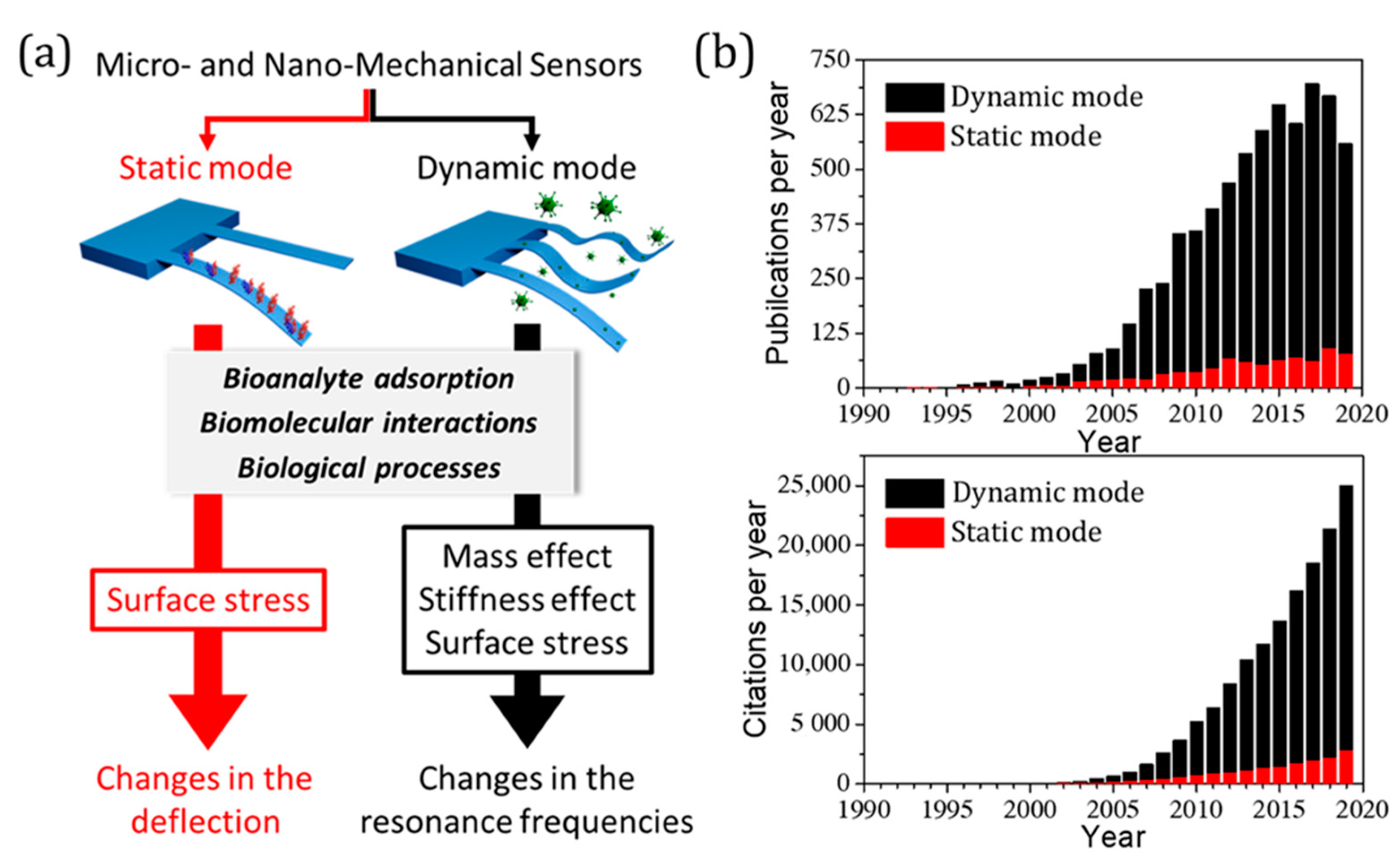
Regarding the working principle, nanomechanical sensors, which are based on the study of the deformation of flexible structures at the nanoscale, can be split into two main groups: static mode and dynamic mode sensors [16,17] (Figure 1a). While the static mode is based on detecting changes in the deformation state of the sensor, the dynamic one is based on detecting changes of the mechanical resonances of such flexible structures. Although the use of both operation modes dates from the mid 1990s, the dynamic mode spread more rapidly, and nowadays, it encompasses around 80% of the research works in this field (Figure 1b).

The physical origin of the signals may come from a wide variety of sources depending on the operation mode and the particular application. Nanomechanical sensors were first applied for the atomic force microscopy (AFM) technique [18,19,20]. AFM serves to reconstruct the topography and physicochemical composition of surfaces at the nanoscale. In this case, the physical origins of the signals that enable characterizing the surfaces deal with the existing interaction forces between the tip of a micro-cantilever and the surface. Nanomechanical sensors comprise biological applications at every scale [21], going from monitoring vital signs to proteomics. At the macroscale, they have been applied for monitoring the corporal temperature [22], the heart rate [23], the respiratory rhythm, the blood pressure, and the level of sucrose in blood. Going down to the micro- and nanoscale, nanomechanical sensors can characterize the motion and forces associated with biomolecular processes and detect and identify the presence of biological entities at extremely low concentrations based on their mass and mechanical properties. In these cases, each operation mode is based on very different detection principles [24,25]. The static mode relies on inducing differential surface stress on the sensor [26,27,28], which is commonly a thin micro-cantilever. One surface of the sensor is functionalized with molecular receptors that exhibit high affinity to targeted molecules [14,29]. As molecular recognition takes place, differential surface stress leads to the deflection of the sensor. On the other hand, the dynamic mode relies on inducing changes on the sensor mechanical properties [30,31]. In most cases, these changes are associated with the addition of mass. In this operation mode, every surface of the sensor can be functionalized. When molecular recognition occurs, mass addition modifies the sensor resonance frequencies. Although cantilever beams are also a common choice for the sensor in this case, many other forms can be frequently found in the literature, from nanowires to membranes or more complex resonant structures [32,33,34,35]. One important aspect of nanomechanical sensors when applied to biological detection is that energy dissipation hampers their capabilities, such as their sensitivity and limit of detection. When immersed in fluids, dynamic nanomechanical sensors suffer a great amount of energy dissipation caused by the density and viscosity of the surrounding fluid. Thus, for liquids, the natural environment of biology, reducing energy dissipation constitutes a very important task. In order to circumvent this problem, researchers have suggested the application of many novel devices and techniques, such as the use of channeled [36,37,38,39] or partially immersed resonators [40], monitoring higher order modes [41], modes with less dissipation [42], or implementing active feedback loops [43], among many others. To date, the ones providing better results are the channeled resonators [44]. These devices comprise internal channels through which the liquid flows. Such configuration significantly mitigates the energy dissipation caused by the presence of the fluid, keeping the sensors’ capabilities unaltered. Unfortunately, it is very difficult to miniaturize channeled devices because their associated microfluidic resistance rapidly increases, and because of limitations in the fabrication process. More recently, researchers have suggested the application of optomechanical platforms [45,46,47,48,49,50,51] as an encouraging alternative. Optomechanics provide access to mechanical modes that possess extraordinary properties, in terms of sensitivity and speed, even when immersed in the most dissipative fluids.

Since their origin, experimentalists and theorists have worked closely, aiming at the implementation of more sensitive, rapid, effective, robust, and integrable devices. In this spirit, advances in micro and nanofabrication techniques have enabled the production of continuously smaller devices, made of plenty of different materials and geometries. Together with the rapid evolution of the devices, researchers have made a huge effort in developing more accurate theoretical models, which enable accessing the basic principles that govern their applications and allow the correct interpretation of the sensors’ signals, providing access to more, and more precise, information about the particular entities or processes of interest. Moreover, theory is essential to assist the design of the devices, as it serves to predict their capabilities regarding a given application, as well as their intrinsic sensitivities and their fundamental limits of detection [52]. This article focuses on the evolution of theoretical modeling in the field of nanomechanical sensing for biological applications, particularly gathering the most popular theoretical models currently applied.

Theories and models for the static operation mode date as far back as 1909, when G.G. Stoney published his formula to relate the surface stress with the bending curvature of a free plate [53]. Although this formula was not intended for biological applications, it later became the basis for the surface stress calculation due to a biological layer adsorption on a plate [14,54,55,56]. However, this formula did not account for the clamping effect of cantilevers. Much later, Sader et al. proposed a solution for a cantilever plate in the asymptotic limits of high and low aspect ratio of the plate [57]. Some years later, Tamayo et al. obtained very simple solutions for the transversally averaged curvatures of the plate that can be used to calculate the surface stress from the experimental measurements of the cantilever deflection in a very easy way [58]. Regarding the dynamic mode, the first time that the use of the change in frequency of a resonator for bio-sensing applications was published was in 1997 in a work presented by Thundat et al. [59]. Three years later, in 2000, Ilic et al. demonstrated the detection of Escherichia coli bacteria using an array of low-stress silicon nitride resonant cantilevers [60], where they used simple formulas to relate the change in frequency to the mass of the analyte. This change was inversely proportional to the mass of the sensor and directly proportional to the mass of the analyte, and it was calculated for a homogeneous layer of material adsorbed on the cantilever surface. For small particles, the adsorption position plays a crucial role and must be known in order to calculate the mass of the analyte correctly. In 2005, Dohn et al. proposed a method to calculate the mass and position of the adsorbed particle using different modes of vibration [41] and, years later, in 2012, Hanay et al. proposed a method for the same task based on probability density functions [9]. In 2006, Ramos et al. proposed a model where, not only the mass, but also the stiffness effect of the analyte on the resonant frequency of the cantilever was accounted for [30]. This model did not account for the edge effects of the analyte, which were finally included by Ruz et al. in 2014 [61] and in a more general framework in 2020 [62]. These and other theoretical models that will be revised and explained later in the text can be considered as the basic theory for the field of nanomechanical sensing for biological applications.

As we have emphasized, nanomechanical sensors can provide very valuable information about a very broad variety of physical properties of the biological entities or processes under study. Theoretical models are essential to properly process this information, as well as to design more sensitive and effective sensors. In this review, we aim to summarize the main theoretical models applied in this field. We first address the static operation mode and then we move to show basic principles and models of the dynamic mode. We then focus on particular models applied when nanomechanical sensors operate in liquids. In each section, the theoretical models increase in complexity, in the same way as they evolve along the history.

2. Nanomechanical Sensors in Static Mode: Effect of Surface Stress

The static bending of a thin plate can be caused by an applied force perpendicular to the plate plane or by a bending moment. The latter can be produced by different means. For instance, a plate formed by two layers of different materials will suffer bending whenever it is exposed to a temperature change because of the different thermal expansion coefficients of the two layers [63,64]. Larger temperature changes will produce larger bending on the plate, thus the static bending of the plate can be directly related to the temperature change, making it a highly sensitive temperature sensor [13,65,66]. A similar phenomenon occurs when one face of the plate is covered by a layer of a biological material [25,67,68]. The interaction forces between molecules within the biological layer produce surface stress on the face of the plate [69,70,71]. If the other face of the plate is uncovered, the difference of surface stress between the upper and lower faces of the plate will produce a bending moment that is proportional to the difference of surface stress between the two faces, or in this case, to the surface stress generated by the biological layer. In order to extract the surface stress from the measurement of the bending of the plate, the relation between the bending and the surface stress must be known. The differential equation that governs the bending of a rectangular plate is the so-called biharmonic equation, which, in Cartesian coordinates, is given by [72]

$$\frac{{\partial }^{4}w\left(x,y\right)}{\partial x^4}+2\frac{{\partial }^{4}w\left(x,y\right)}{\partial x^2\partial y^2}+\frac{{\partial }^{4}w\left(x,y\right)}{\partial y^4}=0$$

(1)

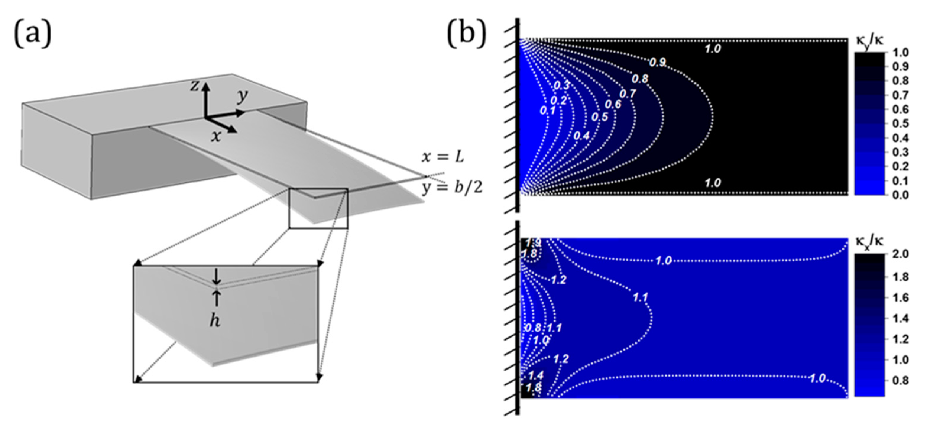
where $w\left(x,y\right)$ is the out-of-plane displacement of the plate, which is set to be along the $z$ coordinate direction. Equation (1) assumes that there are no net external forces applied to the plate. Let us consider a rectangular plate of length $L$, width $b$, and thickness $h$ (Figure 2a). The most common cases of boundary conditions are free and clamped. When there is a bending moment $M$ applied to the plate, the free boundaries satisfy the following conditions:

$$\frac{E_c{h}^3}{12\left(1-{\nu }^2\right)}\left(\frac{{\partial }^{2}w\left(x,y\right)}{\partial n^2}+\nu \frac{{\partial }^{2}w\left(x,y\right)}{\partial s^2}\right)=M$$

(2)

$$\frac{{\partial }^{3}w\left(x,y\right)}{\partial n^3}+\left(2-\nu \right)\frac{{\partial }^{3}w\left(x,y\right)}{\partial s^2\partial n}=0$$

(3)

where $n$ and $s$ refer to the components normal and parallel to the boundary, respectively, and $E_c$ and $\nu$ are the Young’s modulus and Poisson ratio of the plate, respectively. The first to obtain the solution of Equation (1) together with boundary conditions (2) and (3) and relate it to the difference of surface stress between the upper and lower faces of the plate was George Gerald Stoney in 1909 [53]. The solution is a quadratic function of $x$ and $y$ and can be expressed as

$$w\left(x,y\right)=\frac{6\left(1-\nu \right)M}{E_c{h}^3}\left(x^2+y^2\right)$$

(4)

Equation (4) states that the curvature produced by the differential surface stress is constant throughout the whole plate.

The bending moment is related to the differential surface stress $\Delta \sigma$ as $M=\frac{h}{2}\Delta \sigma$. Therefore, the curvature of the plate $\kappa$ can be expressed as

$$\kappa =\frac{6\left(1-\nu \right)}{E_c{h}^2}\Delta \sigma$$

(5)

Equation (5) is the well-known Stoney’s equation and has been used to quantify the differential surface stress on plates since it was first published in 1909. However, for biological applications, it is common to use a plate in a cantilever configuration, i.e., one of the edges is clamped so that its movement is completely restricted. Assuming the clamped edge at $x=0$, the boundary conditions for a clamped edge are

$$w\left(0,y\right)=0$$

(6)

$$\frac{\partial w\left(0,y\right)}{\partial x}=0$$

(7)

Solution (4) is not valid anymore for a cantilever plate and Stoney’s equation loses accuracy to describe the curvature, especially near the clamping region (Figure 2b). Because of the lesser influence of the clamped edge, it is obvious that Stoney’s equation will describe better the curvature for high aspect ratio cantilevers. The analytical solution of Equation (1) with cantilever boundary conditions was attempted by Zeng et al. [73]. They proposed a solution in the form of an infinite series of hyperbolic and trigonometric functions. However, the calculation of the coefficients of the series requires solving an ill-conditioned infinite system of equations with slow convergence, which suggests the clamped boundary condition and the free boundary conditions are in conflict at the common corners. John Elie Sader [57] found approximated solutions to the problem in the asymptotic limits of high and very low aspect ratios. For $L\gg b$, Sader’s solution takes the following form:

$$w\left(x,y\right)=\frac{\kappa }{2}\left(x^2+y^2\right)+g_1\left(x\right)+y^2{g}_2\left(x\right)$$

(8)

where the functions $g_1\left(x\right)$ and $g_2\left(x\right)$ are given by

$$g_1\left(x\right) =-\frac{\kappa b^2}{2}\left(\frac{1}{12}+2\nu \left(\frac{1}{{\tau }_1^2}+\frac{1}{{\tau }_2^2}+\frac{1}{{\tau }_1{\tau }_2}-\frac{x}{b}\left(\frac{1}{{\tau }_1}+\frac{1}{{\tau }_2}\right)\right)+{\displaystyle \sum }_{1=1}^2\frac{{\tau }_{3-i}}{{\tau }_{3-i}-{\tau }_i}\left(\frac{1}{12}+\frac{2\nu }{{\tau }_i^2}\right)e^{-{\tau }_i\frac{x}{b}}\right)$$

(9)

$$g_2\left(x\right)=-\frac{\kappa }{2}{\displaystyle \sum }_{1=1}^2\frac{{\tau }_{3-i}}{{\tau }_{3-i}-{\tau }_i}{e}^{-{\tau }_i\frac{x}{b}}$$

(10)

where the coefficients ${\tau }_i$ depend on the Poisson’s ratio and are given by

$${\tau }_i =2\sqrt{3}\sqrt{5\left(1-\nu \right)+{\left(-1\right)}^i\sqrt{10\left(1-\nu \right)\left(2-3\nu \right)}}$$

(11)

Equation (8) states that the curvature of the cantilever follows Stoney’s equation far from the clamped edge and then decays exponentially with a characteristic length of the order of $b$ as we approach the clamped edge.

A different approach was published by Tamayo et al. [58] for cantilevers with aspect ratio $\frac{L}{b}>1$. They obtained solutions for the averaged curvatures along the transversal coordinate $y$. In this manner, the clamped boundary conditions are relaxed and the conflict at the corners disappears. They obtained very simple formulas for the averaged transversal and longitudinal curvatures:

$${\overline{\kappa }}_x =\kappa \left(1+\nu e^{-\frac{x\alpha }{b}}\right)$$

(12)

$${\overline{\kappa }}_y=\kappa \left(1-e^{-\frac{x\alpha }{b}}\right)$$

(13)

where the coefficient $\alpha$ depends on Poisson’s ratio and is given by

$$\alpha \approx 2.28+1.01\nu -0.18{\nu }^2$$

(14)

Equations (12) and (13) are extremely simple and can be used to calculate $\kappa$ with very high precision from the experimental measurement of the cantilever deflection.

3. Nanomechanical Sensors in Dynamic Mode

Nanomechanical sensors have different modes of vibration, each one associated to its corresponding resonance frequency [74]. Although the resonator is a mechanical structure made of a continuum material and its movement should be described by the theory of elasticity, for certain applications, it is possible to model it as a harmonic oscillator with a certain effective mass ($m_{effn})$ and spring constant ($k_n)$. In this manner, the resonance frequencies can be defined as

$$f_n=\frac{1}{2\pi }\sqrt{\frac{k_n}{m_{effn}}}$$

(15)

Let us define an external perturbation, which can be of very different nature, from temperature, pressure, or humidity changes to force gradients, adsorption of individual molecules, or surface stress produced by a complete layer. This perturbation can change the elastic constant or the effective mass of the resonator, causing a shift in the resonance frequencies. These changes can be measured and carry valuable information about the external perturbation itself. This basic principle has allowed the nanomechanical sensors in dynamic mode to become an extremely useful tool for detecting biological entities and measuring its mechanical properties. In this section, we will review the theoretical models for the effect of the adsorption of analytes such as individual particles, as well as complete layers, on the resonance frequencies of the nanomechanical resonator, the two main effects used for biological applications.

3.1. Effect of a Complete Layer

There are two different effects that arise from the adsorption of a layer of biological material on the resonator surface. The first one is the surface stress produced by the interactions between the molecules that formed the adsorbed layer. The second is the result of the added mass and stiffness due to this new layer of material.

3.1.1. Effect of Surface Stress

As we have mentioned before, surface stress generated by a biological layer on one of the faces of a cantilever plate can be obtained by measuring the static deflection [75]. However, surface stress also alters the dynamics of the plate, even if both faces are covered with the biological material and there is no bending at all. When a string is under tension, it vibrates at higher frequencies because the net force increases the effective stiffness of the string. Similarly, for a doubly clamped beam with a net surface stress applied ${\sigma }^T$, the frequency of the beam increases proportionally to the surface stress and the relative frequency shift for the fundamental mode can be expressed as [76,77]

$$\begin{array}{c}\frac{\Delta f}{f_0} =\frac{1-\nu }{E_{c}h}\left(0.1475{\left(\frac{L}{h}\right)}^2+\frac{\left(1+\nu \right)\left(1+2\nu \right)}{1-\nu }\right){\sigma }^T\end{array}$$

(16)

where $f_0$ and $f$ are the resonance frequencies before and after deposition, respectively. However, cantilever plates can release the stress through the free edge, thus it is reasonable to think that the frequency will not change with surface stress. Whether or not surface stress affects the frequency of cantilever plates has generated a long debate among scientists of the field for the last decades [78,79,80,81]. Recent experimental studies have clearly shown that surface stress influences the stiffness of cantilever plates, changing the resonant frequency [76,82], and several theoretical models have been proposed to explain this phenomenon. At this point, it is important to distinguish between net surface stress, which is the sum of the surface stress on the upper and lower faces of the cantilever plate, and differential surface stress, which is the difference between the surface stresses of both faces. A net surface stress produces in-plane deformation of the cantilever, while a differential surface stress produces bending. A theoretical model to describe the effect of net surface stress on cantilevers was proposed by Lachut et al. [77,83]. In these works, they showed that there are two different effects, one coming from the geometrical changes of the structure due to the stress release and another one from the fact that the clamped edge cannot release the stress along the transversal direction, thus a residual stress is accumulated near the clamping region, affecting the resonant frequency of the cantilever plate. They proposed a formula for the relative frequency shift of the fundamental mode of cantilevers:

$$\begin{array}{c}\frac{\Delta f}{f_0} =\frac{1-\nu }{E_{c}h}\left(-0.042\nu \frac{b^3}{L{h}^3}+\frac{1+2\nu }{1-\nu }\right){\sigma }^T\end{array}$$

(17)

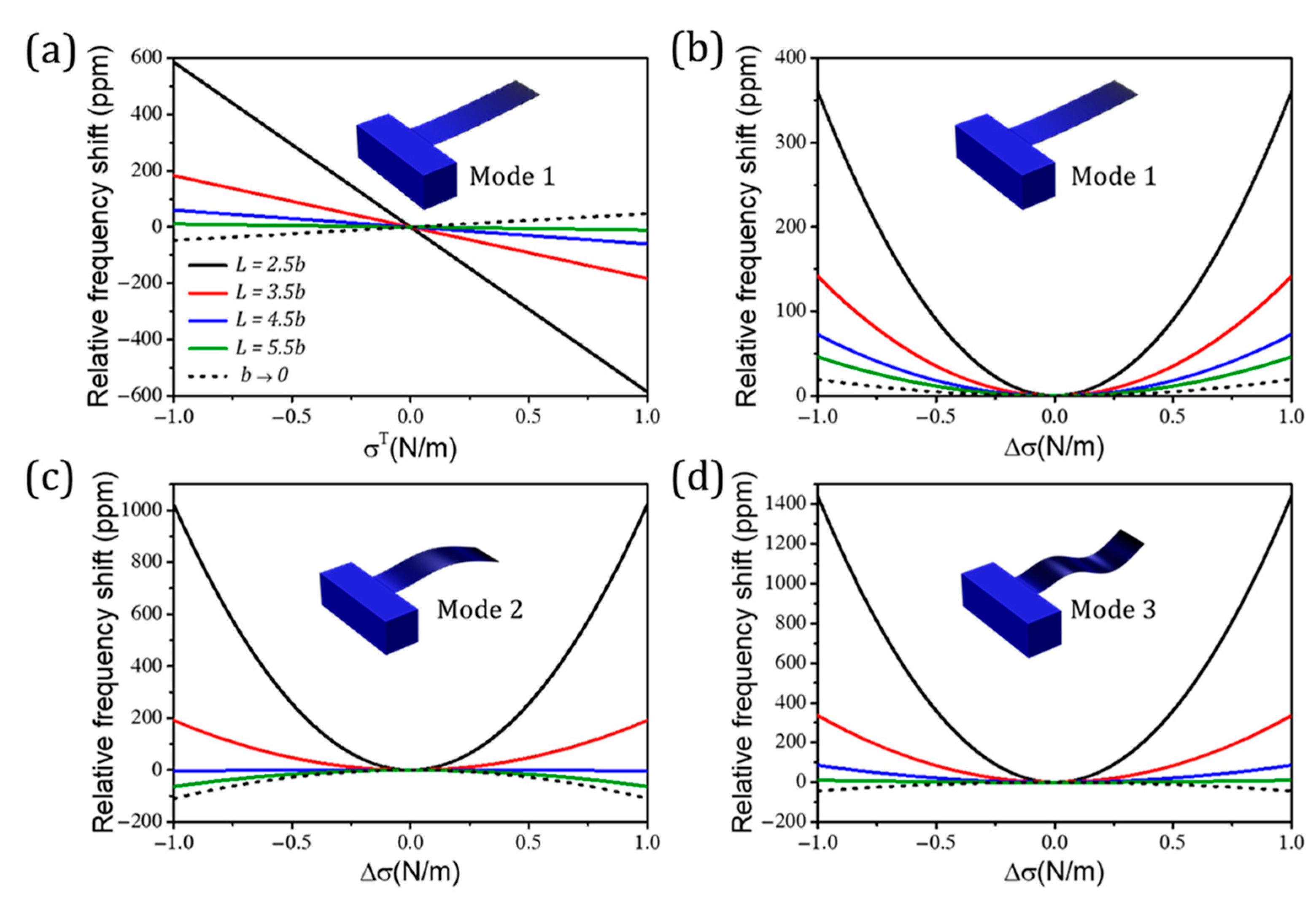
As an example, Figure 3a shows the relative frequency shift due to net surface stress for a silicon nitride cantilever with a thickness of 100 nm and length of 20 µm, for different values of the aspect ratio, and as a function of the net surface stress. Equation (17) is formed by two terms that correspond to the two different effects described above. The geometric term is inversely proportional to the thickness of the cantilever, while the residual stress term is proportional to $\frac{b^3}{L{h}^3}$. It is interesting to note that these two effects have opposite signs; therefore, a cantilever could be designed with specific characteristics in order to avoid net surface stress effects on the frequency or, on the other hand, to maximize the effect in order to have a better measurement of the surface stress.

More recently, a theoretical framework to describe the effect of differential surface stress on the stiffness of cantilever plates has been developed [84,85]. In these works, it was found that two-dimensional bending of thin plates leads to the development of in-plane stresses that highly increase the flexural stiffness of the plate. In addition, a nonlinear effect due to large static bending was also included in the theoretical model. The equation of the effect of differential surface stress on the relative frequency shift of cantilever plates for the first three flexural modes of vibration is given by

$$\begin{array}{c}\frac{\Delta f_n}{f_{n_0}} =\end{array}\frac{36{\left(1-\nu \right)}^2{L}^2}{E_c{}^2{h}^4}\left({\alpha }_n+\frac{1}{120}{\left(\frac{L}{h}\right)}^2{\left(\frac{b{e}^{-c\frac{b}{L}}}{L}\right)}^4\left({\left(1-\nu \right)}^2-2\nu +{\mathsf{\Lambda }}_n\left(\nu \right){\left(\frac{b{e}^{-c\frac{b}{L}}}{L}\right)}^2\right)\right)\Delta {\sigma }^2$$

(18)

where $c=0.7745$ is a constant, and the coefficient ${\alpha }_n$ accounts for the nonlinear effect due to large static bending and takes the values of $\approx 0.02029, -0.11553, \mathrm{and} -0.04670$ for the first, second, and third flexural modes, respectively. The function ${\mathsf{\Lambda }}_n\left(\nu \right)$ can be approximated by a second-order polynomial of Poisson’s ratio for the first three flexural modes:

$$\begin{array}{c}\left(\begin{array}{c}{\mathsf{\Lambda }}_1\\ {\mathsf{\Lambda }}_2\\ {\mathsf{\Lambda }}_3\end{array}\right) =\end{array}\left(\begin{array}{ccc}-0.33& 8.82& -29.31\\ 10.83& -26.77& -11.45\\ 8.13& -3.22& -29.80\end{array}\right)\left(\begin{array}{c}1\\ \nu \\ {\nu }^2\end{array}\right)$$

(19)

The two-dimensional bending effect is proportional to $\frac{b^4}{h^6}$; therefore, it will be the dominant effect for very thin plates. On the other hand, as the aspect ratio of the cantilever increases and the nonlinear term becomes more important until, finally, in the asymptotic limit $\frac{L}{b}\gg 1$, the two-dimensional bending term is negligible with respect to the nonlinear term. Figure 3b–d show the relative frequency shift due to differential surface stress for a silicon nitride cantilever with a thickness of 100 nm, length of 20 µm, and different values of the aspect ratio as a function of the differential surface stress for the first three flexural modes.

3.1.2. Mass and Stiffness Effects

When a homogeneous layer of a material is deposited on one of the surfaces of the sensor, the total mass of the system increases, thus the resonance frequency must decrease in order to maintain the energy balance [86]. However, the new layer deforms along with the resonator, increasing the strain energy of the system, thus the resonance frequency must increase in order to keep the mechanical energy constant. Depending on the properties of the new layer, it might even change the strain distribution inside the resonator, considerably moving the neutral axis towards the adsorbed layer. In a nutshell, the mass effect produces a decrease in the resonance frequency and the stiffness effect produces an increase in the resonance frequency. For a general layer, the relative change in frequency for any flexural mode of a cantilever sensor can be expressed as

$$\frac{f^2-f_0{}^2}{f_0{}^2}=-\frac{\eta {\rho }_a}{\eta {\rho }_a+{\rho }_c}+\frac{\eta \frac{E_a}{E_c}{\rho }_c\left(3+6\eta +4{\eta }^2+\frac{E_a}{E_c}{\eta }^3\right)}{\left(\eta {\rho }_a+{\rho }_c\right)\left(1+\eta \frac{E_a}{E_c}\right)}$$

(20)

where $\rho$ is the density; $\eta$ is the ratio between the thickness of the layer and the thickness of the cantilever; and subscripts $a$ and $c$ refer to analyte and cantilever, respectively. It must be noticed that Equation (20) is valid for both cantilever plates and doubly clamped beams. One important feature of Equation (20) is that the relative change in frequency does not depend on the mode of vibration; therefore, it is the same for any flexural mode. This is a particular characteristic of the adsorption of homogeneous layers that cover the whole surface of the resonator. For a thin layer of a biological material where $\eta \ll 1$ and $E_a\ll E_c$, Equation (20) can be simplified and the relative frequency shift can be approximated by

$$\frac{\Delta f}{f_0}\cong \eta \left(-\frac{{\rho }_a}{2{\rho }_c}+\frac{3E_a}{2E_c}\right)$$

(21)

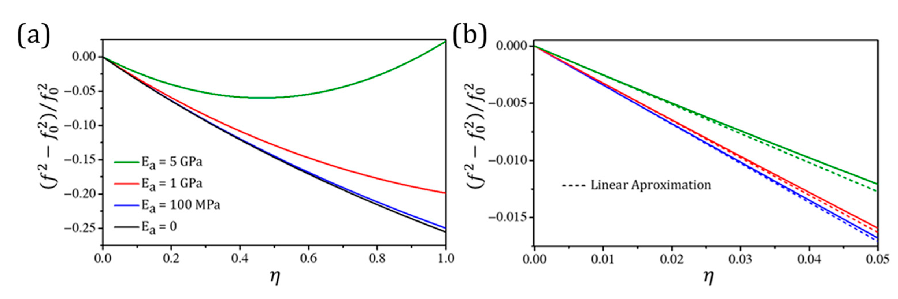
where we have considered that the change in frequency is small and, therefore, $\frac{\Delta f}{f_0}\cong \frac{1}{2}\frac{f^2-f_0{}^2}{f_0{}^2}$. Figure 4 shows the relative frequency shift as a function of $\eta$ due to the adsorption of an homogeneous layer of a biological material with density of 800 $\mathrm{kg}/{\mathrm{m}}^3$ on a silicon cantilever for different values of $E_a$.

3.2. Individual Particles

One of the most important applications of nanomechanical resonators is particle identification. Because of its extremely high sensitivity, nanomechanical resonators have allowed the birth of a new type of mass spectrometry known as nanomechanical mass spectrometry [9,10,32,87,88,89,90]. This type of mass spectrometry does not require ionization and fragmentation [90] of the sample, and thus is ideal for biological entities like viruses [32] or bacteria [10]. Like complete layers, individual particles that adsorb on the resonator surface have two opposite effects on the resonance frequency; that is, the mass effect, which decreases the frequency, and the stiffness effect, which increases the frequency. However, unlike complete layers, the frequency shift is in general different for different modes of vibration. The mass effect is associated with the kinetic energy of the adsorbed particle, thus it will be proportional to the square of the mode shape at the adsorption position [24,91]. On the other hand, the stiffness effect is associated with the strain energy of the adsorbed particle as a consequence of the bending of the resonator, thus it will be proportional to the square of the curvature of the mode shape at the adsorption point. The first formula that included the stiffness effect in the relative frequency shift due to the adsorption of a small particle type of analyte was proposed by Ramos et al. [30] and is given by

$$\frac{\Delta f_n}{f_{n_0}}=-\frac{m_a}{2m_c}{\psi }_n{\left(X_0\right)}^2+\frac{3E_a{V}_a}{2E_c{V}_c}(1+2\eta +\frac{4}{3}{\eta }^2)\frac{1}{{\lambda }_n{}^4}{\left(\frac{d^2{\psi }_n\left(X_0\right)}{d{X}^2}\right)}^2$$

(22)

where $V$ is the volume; $X=x/L$ is the longitudinal position normalized to the length of the resonator; $X_0$ is the normalized adsorption position; and ${\psi }_n$. is the nth mode of vibration, given by

$${\psi }_n=cosh\left(X{\lambda }_n\right)-cos\left(X{\lambda }_n\right)+\frac{cos{\lambda }_n\pm cosh{\lambda }_n}{sin{\lambda }_n\pm sinh{\lambda }_n}\left[sin\left(X{\lambda }_n\right)-sinh\left(X{\lambda }_n\right)\right]$$

(23)

where ${\lambda }_n$ is the eigenvalue that satisfies the following equation:

$$1\pm cosh\left({\lambda }_n\right)cos\left({\lambda }_n\right)=0$$

(24)

where the $+$ sign corresponds to cantilevers and the − sign to doubly clamped beams. In Equation (22), the mode of vibration has been normalized so that

$${{\displaystyle \int }}_0^1{\psi }_n{\left(X\right)}^{2}dX=1$$

(25)

However, Equation (22) does not account for the relaxation of the stress through the free edges of the adsorbed particle. This relaxation is very important for small particles with a small surface to volume ratio, thus the stiffness part of Equation (22) is not accurate for this kind of particle. In 2014 [61], the edge effects of the particle were carefully studied and introduced into the stiffness part of Equation (22). These effects are responsible for the dependence of the stiffness effect on the shape, the contact to the cantilever surface, or the angle of orientation of the adsorbed particle with respect to the cantilever main axis. This proposed model includes a stiffness coefficient ${\gamma }_{flex}$ that measures the strain transmission from the cantilever to the adsorbed particle, leading to the following equation for the relative frequency shift:

$$\frac{\Delta f_n}{f_{n_0}}=-\frac{m_a}{2m_c}{\psi }_n{\left(X_0\right)}^2+\frac{3E_a{V}_a}{2E_c{V}_c}{\gamma }_{flex}\frac{1}{{\lambda }_n{}^4}{\left(\frac{d^2{\psi }_n\left(X_0\right)}{d{X}^2}\right)}^2$$

(26)

${\gamma }_{flex}$ can be expressed as a function of the angle of orientation of the particle with respect to the main axis of the cantilever $\theta$, just by applying a rotation along the vertical axis:

$${\gamma }_{flex}={\gamma }_1{cos}^4\left(\theta \right)+{\gamma }_2{sin}^4\left(\theta \right)+{\gamma }_3{cos}^2\left(\theta \right){sin}^2\left(\theta \right)$$

(27)

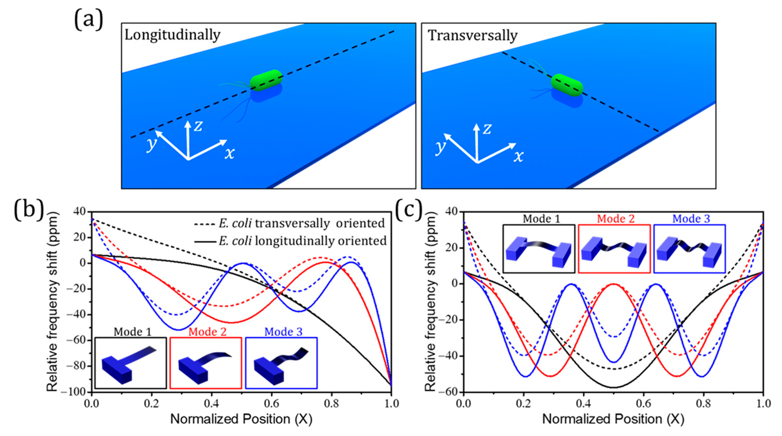
where ${\gamma }_1$, ${\gamma }_2$, and ${\gamma }_3$ are coefficients that depend on the shape of the particle, the radius of contact, and $\eta$. Figure 5 shows the relative frequency shift due to the adsorption of a typical E. coli bacterium on a cantilever and a doubly clamped beam made out of silicon nitride as a function of the adsorption position $X_0$ for the first three flexural modes. As the E. coli bacterium has a cylindrical form, the relative frequency shifts for both longitudinal and transversal orientation were represented.

Recently, a more general framework to describe the stiffness effect of an individual particle adsorbed on a resonant plate of any shape has been developed [62]. In this work, it was found that the coefficient $\gamma$ is actually a fourth-order tensor with major and minor symmetries that can be described by six independent coefficients. The framework describes the relative frequency shift due to the adsorption of a particle on a plate of any shape vibrating at any type of mode, in- or out-of-plane:

$$\frac{\Delta f_n}{f_{n_0}}=-\frac{m_a}{2m_c}\left|{\psi }_n(X_0,Y_0)\right|{ }^2+\frac{E_a{V}_a\left(1-{\nu }^2\right){\gamma }_{mqrs}}{2E_c{V}_c }\frac{{\epsilon }_{mq}\left(X_0,Y_0\right){\epsilon }_{rs}\left(X_0,Y_0\right)}{{\beta }_n^4}$$

(28)

where ${\beta }_n$ is a number related to the eigenvalue of the mode; ${\epsilon }_{mq}\left(X_0,Y_0\right)$ is the strain component $mq$ of the plate at the adsorption position $\left(X_0,Y_0\right)$; the indexes $m,q,r$, and $s$ can take the values $x$ and $y$; and Einstein’s summation of repeated indexes is used. Note that the mode shape is in bold, indicating that it is a vector that, in a general case, can have $x$, $y$, and $z$ components. For flexural modes of cantilevers or doubly clamped beams, Equation (28) reduces to Equation (26). It is interesting to note that the tensor ${\gamma }_{mqrs}$. has two linear invariants to rotations around the vertical axis:

$$I_1={\gamma }_{xxxx}+{\gamma }_{yyyy}+2{\gamma }_{xxyy}$$

(29)

$$I_2={\gamma }_{xxxx}+{\gamma }_{yyyy}+2{\gamma }_{xyxy}$$

(30)

These two quantities are very useful for particle identification applications because, as invariants, they do not depend on the angle of orientation of the particle, a variable that cannot be controlled.

3.2.1. Multimode Measuring

The fact that the relative frequency shift is different for different modes of vibration when an individual analyte is adsorbed on the resonator surface allows for the determination of the adsorption position, mass, and stiffness of the particle just by measuring the relative frequency shift of several modes simultaneously [9,10,32]. This is commonly known as solving the inverse problem. Mathematically, Equation (26) using N modes constitutes a system of N equations with three unknowns, which are ${\Delta }_m=\frac{m_a}{2m_c}$, ${\Delta }_s=\frac{3E_a{V}_a}{2E_c{V}_c}{\gamma }_{flex}$ , and $X_0$. 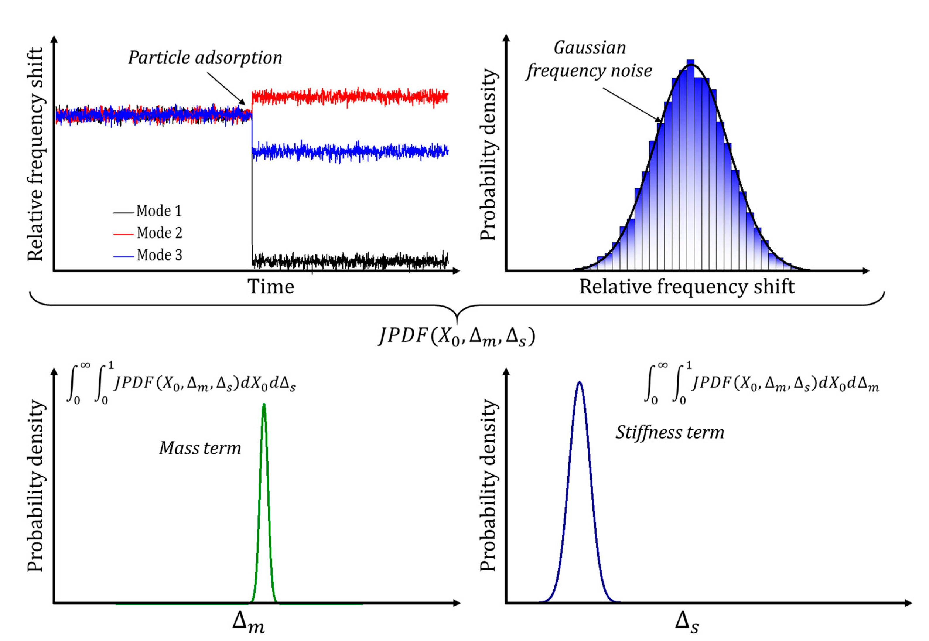In principle, three modes could be enough to solve the problem because we have three unknowns. However, the dependency on the adsorption position $X_0$ is nonlinear, thus the system might have more than one solution. Very different scenarios can occur depending on the adsorption position. For instance, for cantilever beams, ${\Delta }_m$ can never be determined for $X_0=0$ and ${\Delta }_s$ can never be determined for $X_0=1$. Another critical point is $X_0=0.5$, where ${\psi }_n{\left(X\right)}^2=\frac{1}{{{\lambda }_n}^4}{\left(\frac{d^2{\psi }_n\left(X_0\right)}{d{X}^2}\right)}^2$ for any value of $n$. In this case, we can determine ${\Delta }_m+{\Delta }_s$, but never both of them separately. In practice, for real-time applications, the relative frequency shifts can be measured with a certain level of precision that is ultimately determined by the frequency stability of the system [92]. Assuming that the frequency noise is Gaussian, we can express the probability density function (PDF) of the relative frequency shift for the nth mode as follows [9,10]:

$$PDF\left(\frac{\Delta f_n}{f_{n_0}}\right)=\frac{e^{-\frac{{\left(\frac{\Delta f_n}{f_{n0}}-{\Delta }_f^{\left(n\right)}\right)}^2}{2{\sigma }_{Allan}^2}}}{{\sigma }_{Allan}\sqrt{2\pi }}$$

(31)

where ${\Delta }_f^{\left(n\right)}$ is the relative frequency shift measured experimentally and ${\sigma }_{Allan}$ is the Allan deviation of the corresponding frequency for the integration time used in the experiment. For N modes measured simultaneously, we must use the joint probability density function ($JPDF)$ of the PDFs of all the modes. This function is a multi-normal distribution given by

$$JPDF\left(\widehat{\frac{\Delta f}{f_0}}\right)=\frac{e^{-\frac{\left(\widehat{\frac{\Delta f}{f_0}}-{\hat{\Delta }}_f\right){\mathsf{\Sigma }}^{-1}{\left(\widehat{\frac{\Delta f}{f_0}}-{\hat{\Delta }}_f\right)}^T}{2}}}{{\left(2\pi \right)}^{N/2}\sqrt{\left|\mathsf{\Sigma }\right|}}$$

(32)

where $\widehat{\frac{\Delta f}{f_0}}$ is a vector formed by all the relative frequency shift variables, ${\hat{\Delta }}_f$ is a vector formed by all the relative frequency shifts measured experimentally, and $\mathsf{\Sigma }$ is the covariance matrix of the N modes. Obviously, Equation (32) has a maximum for $\widehat{\frac{\Delta f}{f_0}}={\widehat{\Delta }}_f$, and this information is not very useful. However, if $\widehat{\frac{\Delta f}{f_0}}$ is substituted by Equation (26), the new function will depend on the three unknowns of the problem $X_0,{\Delta }_m, {\Delta }_s$. Then, maximization of Equation (32) for the new variables will lead to the solution of the problem. If the number of modes is not enough to obtain a unique solution, the $JPDF$ will display several maxima for different combinations of the variables $X_0,{\Delta }_m, {\Delta }_s$. The precision of the solution will be directly related to the width of the peak of the $JPDF$. Notice that, as a $PDF$, Equation (32) can be integrated in any of the three variables in order to eliminate the dependence on that variable. For instance, if we are interested in the mass probability density function, we can integrate in $X_0$ and ${\Delta }_s$ as follows:

$$JPDF\left({\Delta }_m\right)={{\displaystyle \int }}_0^1{{\displaystyle \int }}_0^{\infty }JPDF\left(X_0,{\Delta }_m,{\Delta }_s\right)d{\Delta }_{s}d{X}_0$$

(33)

Similarly, different probability density functions can be obtained by integrating in the variables in which we are not interested. Figure 6 shows a schematic of the multimode method for the adsorption of a particle on a cantilever beam.

3.2.2. Inertial Imaging

Multimode measuring can also be used to calculate the mass distribution of an analyte that is not considered as a point mass particle. Hanay et al. proposed a formalism based on the calculation of different moments of the mass distribution of the adsorbed particle [87]. The method neglects the stiffness effect of the adsorbed particle and is based on the fact that any polynomial function $p\left(x\right)$ can be approximated by a linear combination of the square of the mode shapes ${\psi }_n$. The relative frequency shift of the nth mode due to the adsorption of a particle that is not considered as a point can be expressed as

$$\frac{\Delta f_n}{f_0}\cong -\frac{1}{2m_c}{{\displaystyle \int }}_0^1{\mu }_a\left(X\right){\psi }_n{\left(X\right)}^{2}dX$$

(34)

where ${\mu }_a\left(X\right)$ is the longitudinal mass distribution of the particle along the beam axis. Equation (34) is reduced to the case of the point-like particle choosing ${\mu }_a\left(X\right)=m_a\delta \left(X-X_0\right)$, where $\delta \left(X-X_0\right)$ is the Dirac delta function. The different moments $m^{\left(k\right)}$ of the mass distribution of the adsorbed particle are defined as

$$m^{\left(k\right)}={{\displaystyle \int }}_0^1{\mu }_a\left(X\right)g^{\left(k\right)}\left(X\right)dX$$

(35)

where $g^{\left(0\right)}\left(X\right)=1$, $g^{\left(1\right)}\left(X\right)=X$, $g^{\left(2\right)}\left(X\right)={\left(X-\frac{m^{\left(1\right)}}{m^{\left(0\right)}}\right)}^2$, and so on. It is clear that $m^{\left(0\right)}$ corresponds to the total mass of the adsorbed particle, $m^{\left(1\right)}/m^{\left(0\right)}$ is the center of mass of the particle or $X_0$, and $m^{\left(2\right)}$/$m^{\left(0\right)}$ is related to the size of the adsorbed particle projected to the $x$ axis. Higher moments can be calculated in the same way and give information about the shape of the particle. In order to calculate these moments from the relative frequency shifts, the functions $g^{\left(k\right)}\left(X\right)$ are expressed as linear combinations of the mode shapes as

$$g^{\left(k\right)}\left(X\right)={\displaystyle \sum }_{n=1}^{\infty }{\alpha }_n^{\left(k\right)}{\psi }_n{\left(X\right)}^2$$

(36)

where ${\alpha }_n^{\left(k\right)}$ are real numbers. Using Equations (34) and (36), the moments $m^{\left(k\right)}$ can be expressed as a function of the relative frequency shift measured experimentally as

$$m^{\left(k\right)}=-2m_c{\displaystyle \sum }_{n=1}^{\infty }{\alpha }_n^{\left(k\right)}\frac{\Delta f_n}{f_0}$$

(37)

In practice, it is not possible to measure infinite modes, however, with a finite number of modes, it is possible to form a good approximation of the functions $g^{\left(k\right)}\left(X\right)$. Of course, the accuracy of the calculation will be higher as more modes are used and the approximation of the functions $g^{\left(k\right)}\left(X\right)$ is better.

4. Hydrodynamic Loading

As stated before, fundamental science and novel applications in technology still need the development of sensors with higher sensitivity and selectivity than the current state-of-the-art accomplishments. In that context, the advances in nanofabrication tools have placed the nanomechanical resonators as the crucial elements of sensing techniques, reaching unprecedented sensitivities. The application idea behind these outstanding sensitivities is the measurement of the changes induced in the mechanical parameters, resonant frequencies, and/or quality factor, of the resonators. However, in order to reach these impressive milestones in the sensing field, researchers are forced to work in highly controlled environments, i.e., ultra-high vacuum conditions and cryogenic temperatures. Hence, the application of these developments is limited to fundamental studies, leaving aside the majority of the biological and chemical reactions that take place in physiological environments. This is because the performance of nanomechanical resonators is heavily deteriorated in liquids, mainly owing to the double side effect of viscous environments [93,94,95,96]; the effective mass of the resonator is dramatically increased because of the dragged mass of the displaced fluid during the oscillation period and the viscous damping degrades the mechanical quality factor. Therefore, in recent years, there has been a great effort by the scientific community to elucidate new ways to combine the excellent dynamical properties of resonators oscillating in vacuum and the new sensing scenarios offered by the sensors operated in liquids. Here, we are going to distinguish between two different operation modes: the operation of the nanomechanical resonator immersed in liquid and the developments of suspended nano- and micro-channels, where the liquid flows inside the resonator, which is placed into a vacuum chamber.

4.1. Nanomechanical Resonators Immersed in Fluid

According to previous studies [97,98,99], the frequency dependence of the damping force for an oscillator immersed in a viscous fluid is related to the well-known hydrodynamic force, i.e., the force that the fluid exerts on the oscillator. For a cantilever beam vibrating in a fluid, the dominant geometric parameter is the width and the hydrodynamic force in the frequency domain can be expressed as

$${\widehat{F}}_{hydro}\left(x,f\right)={\pi }^3{\rho }_f{f}^2{b}^2\mathsf{\Gamma }\left(f\right)\widehat{w}\left(x,f\right)$$

(38)

where $\widehat{w}$ is the out-of-plane displacement; $f$ is the frequency; ${\rho }_f$ is the density of the fluid; and $\mathsf{\Gamma }\left(f\right)$ is the hydrodynamic function that, for a circular cross section, can be obtained analytically [100] and can be written as

$$\mathsf{\Gamma }\left(\omega \right)=1+\frac{4i{K}_1\left(-i\sqrt{ire}\right)}{\sqrt{ire}{K}_0\left(-i\sqrt{ire}\right)}$$

(39)

where $i=\sqrt{-1}$, $K_0$, and $K_1$ are the modified Bessel functions of the third kind and $re={\rho }_{f}f\pi b^2/2{\eta }_f$ is the Reynolds number, where ${\eta }_f$ is the viscosity of the fluid. However, for a rectangular cross section, the solution is not analytical. The previous function can be corrected by a geometrical factor $\mathsf{\Omega }\left(\omega \right)$ so that the new hydrodynamic function is expressed as the product of the geometrical factor and the hydrodynamic function for a circular cross section: ${\mathsf{\Gamma }}_{rec}\left(f\right)=\mathsf{\Omega }\left(f\right)\mathsf{\Gamma }\left(f\right)$. This geometrical factor $\mathsf{\Omega }\left(\omega \right)$ was calculated in [99] as a rational function of ${\log }_{10}re$ for a range $re\in \left[{10}^{-6}, {10}^4\right]$. The real and imaginary parts of $\mathsf{\Omega }\left(f\right)$ can be expressed as

$${\mathsf{\Omega }}_r\left(f\right)=\frac{0.91324-0.48274\tau +0.46842{\tau }^2+0.12886{\tau }^3+0.044055{\tau }^4-0.0035117{\tau }^5+0.00069085{\tau }^6}{1-0.56964\tau +0.48690{\tau }^2-0.13444{\tau }^3+0.045155{\tau }^4-0.0035862{\tau }^5+0.00069085{\tau }^6}$$

(40)

$${\mathsf{\Omega }}_i\left(f\right)=\frac{-0.024134-0.029256\tau +0.016294{\tau }^2+0.00010961{\tau }^3+0.000064577{\tau }^4-0.000044510{\tau }^5}{1-0.59702\tau +0.55182{\tau }^2-0.18357{\tau }^3+0.079156{\tau }^4-0.014369{\tau }^5+0.0028361{\tau }^6}$$

(41)

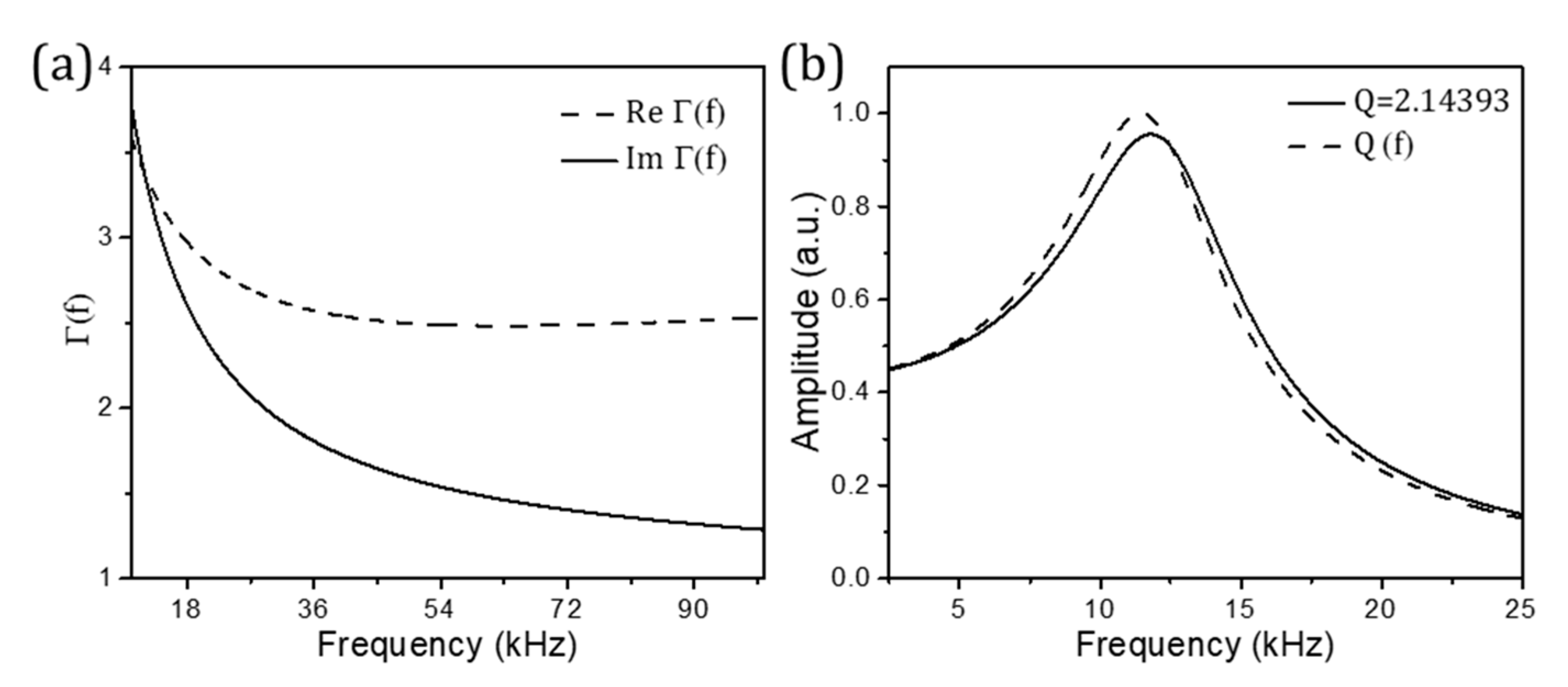
where $\mathsf{\tau }={\log }_{10}re$. Figure 7a shows the real and imaginary parts of the hydrodynamic function of a rectangular cantilever of 200 μm by 20 μm typically used in sensing applications.

The movement of the cantilever in the fluid is impeded by two different mechanisms: the added mass ($m_{ad}$) of the fluid displaced by the resonator during its oscillation cycle and the damping factor (${\gamma }_f$). By expanding the hydrodynamic force into its real and imaginary parts, it is possible to obtain both factors [98,101] in terms of the hydrodynamic function:

$${\gamma }_f=\frac{{\pi }^2}{2}{\rho }_f{b}^{2}LfIm\left[{\mathsf{\Gamma }}_{rec}\left(f\right)\right]$$

(42)

$$m_{ad}=\frac{\pi }{4}{\rho }_f{b}^{2}LRe\left[{\mathsf{\Gamma }}_{rec}\left(f\right)\right]$$

(43)

where $Re$ and $Im$ account for the real and imaginary, parts respectively, and in order to calculate Equations (42) and (43), the normalization condition (25) was applied to the mode shape of the cantilever. Considering these results, we can model the cantilever movement immersed in the fluid as a damped harmonic oscillator as follows:

$$\left[\left(m_c+m_{ad}\left(f\right)\right)\frac{d^2}{d{t}^2}+{\gamma }_f\left(f\right)\frac{d}{dt}+k_{effn}\right]w\left(t\right)=F_{th}\left(t\right)$$

(44)

where $F_{th}\left(t\right)$ is the non-correlated Langevin thermal force and $k_{effn}$ is the effective spring constant of the cantilever, given by

$$k_{effn}=\frac{1}{12}\frac{E_{c}b{h}^3}{L^3}{{\displaystyle \int }}_0^1{\left(\frac{d^2{\psi }_n\left(X\right)}{d{X}^2}\right)}^{2}dX$$

(45)

The resonance frequency and quality factor can be approximated by the following expressions [99]

$$f_{R,n}=f_{vac,n}{\left(1+\frac{\pi {\rho }_{c}b}{4{\rho }_{f}h}Re\left[{\mathsf{\Gamma }}_{rec}\left(f_{R,n}\right)\right]\right)}^{-1/2}$$

(46)

$$Q_n=\frac{\frac{4{\rho }_{c}h}{\pi {\rho }_{f}b}+Re\left[{\mathsf{\Gamma }}_{rec}\left(f_{R,n}\right)\right]}{Im\left[{\mathsf{\Gamma }}_{rec}\left(f_{R,n}\right)\right]}$$

(47)

where $f_{R,n}$ is the nth resonance frequency of the cantilever immersed in fluid, $f_{vac,n}$ is the corresponding resonance frequency in vacuum, and $Q_n$ is the quality factor. Looking at the different parameters in Equation (44), we realize that the mass and the damping factor are not constants anymore; there is a functional dependency with the frequency by means of the hydrodynamic function. Thus, the behavior of a nanomechanical resonator immersed in liquid is not the same as the one oscillating in vacuum with a lower frequency and quality factor. Figure 7b shows the resonant peak for a constant quality factor (solid line) and for the quality factor in Equation (47) (dashed line).

The hydrodynamic function ${\mathsf{\Gamma }}_{rec}\left(f\right)$ mentioned above was obtained for a cantilever with $L\gg b$. The accuracy of this function decreases as $b/L$ increases, especially for higher order modes. However, an improvement of the hydrodynamic function was proposed in order to increase the accuracy for these cases [100]. The hydrodynamic function for a finite aspect ratio and higher order modes can be calculated by solving a system of linear equations that depend on the mode order and on the aspect ratio of the cantilever:

$${\mathsf{\Gamma }}_{rec}\left(f,n\right)=8a_1$$

(48)

where the coefficient $a_1$ can be calculated solving the following system of linear equations:

$${\displaystyle \sum }_{m=1}^p\left(A_{q,m}^{{\kappa }_n}+A_{q,m}^{\mathrm{re}}\right)a_m=\{\begin{array}{cc}1,& q=1\\ 0,& q>1\end{array}$$

(49)

where ${\kappa }_n={\lambda }_n\frac{b}{L}$ and the coefficients $A_{q,m}^{\kappa }$ and $A_{q,m}^{\mathrm{Re}}$ are given by

$$A_{q,m}^{{\kappa }_n}=-\frac{4^{2q-1}}{\sqrt{\pi }}{G}_{13}^{21}\left(\begin{array}{cc}{\frac{{\kappa }_n{}^2}{16}|}_0& \begin{array}{c}3/2\\ \begin{array}{cc}q+m-1& q-m+1\end{array}\end{array}\end{array}\right)$$

(50)

$$\begin{array}{cc}{A}_{q,m}^{\mathrm{re}}=& -{\kappa }_n{}^2\frac{2^{4q-5}}{\sqrt{\pi }}{G}_{13}^{21}\left(\begin{array}{cc}{\frac{{\kappa }_n{}^2-i4\mathrm{re}}{16}|}_0& \begin{array}{c}\frac{1}{2}\\ \begin{array}{cc}q+m-2& q-m\end{array}\end{array}\end{array}\right)\\ & -\frac{2^{4q-1}}{\sqrt{\pi }}{G}_{13}^{21}\left(\begin{array}{cc}{\frac{{\kappa }_n{}^2-i4\mathrm{re}}{16}|}_0& \begin{array}{c}\frac{1}{2}\\ \begin{array}{cc}q+m-1& q-m+1\end{array}\end{array}\end{array}\right)\end{array}$$

(51)

where $G_{13}^{21}$ are Meijer functions and the integer $p$ is to be increased until convergence is achieved.

4.2. Suspended Microchannel Resonators

The current state-of-the-art nanofabrication capabilities allow the development of micro-channels, where the liquid flows inside the resonator, which is placed into a vacuum chamber [38,102]. This is the most promising technique for nanomechanical sensing in liquid environments. Using this configuration, the nanomechanical resonator retains the good mechanical properties of a resonator in vacuum (high frequency and mechanical quality factor), while allowing the sensing in physiological environments, which is crucial for most biological or chemical reactions [103]. These new accomplishments allow to decrease the minimum detectable mass to reach tens of attograms resolution in liquid [104]. However, these hollow resonators are not capable of measuring the analyte inertial mass, giving us the so-called buoyant mass. When an analyte is flowing inside a liquid passing through the hollow resonator, the measured frequency shift is the result of the difference between the mass of the displaced volume of the carrier liquid and the mass of the analyte, which could be problematic when trying to distinguish between two different analytes of different materials and/or volumes. This problem has been addressed in previous studies by measuring the analytes while changing the carrier liquid, which means that it is necessary to measure each analyte several times to unambiguously distinguish between two analyte populations. Nevertheless, this technique remains costly, slow, and not user friendly, because, far from being a universal method, for biological analysis, both carrier liquids need to be carefully selected depending on the specific sample.

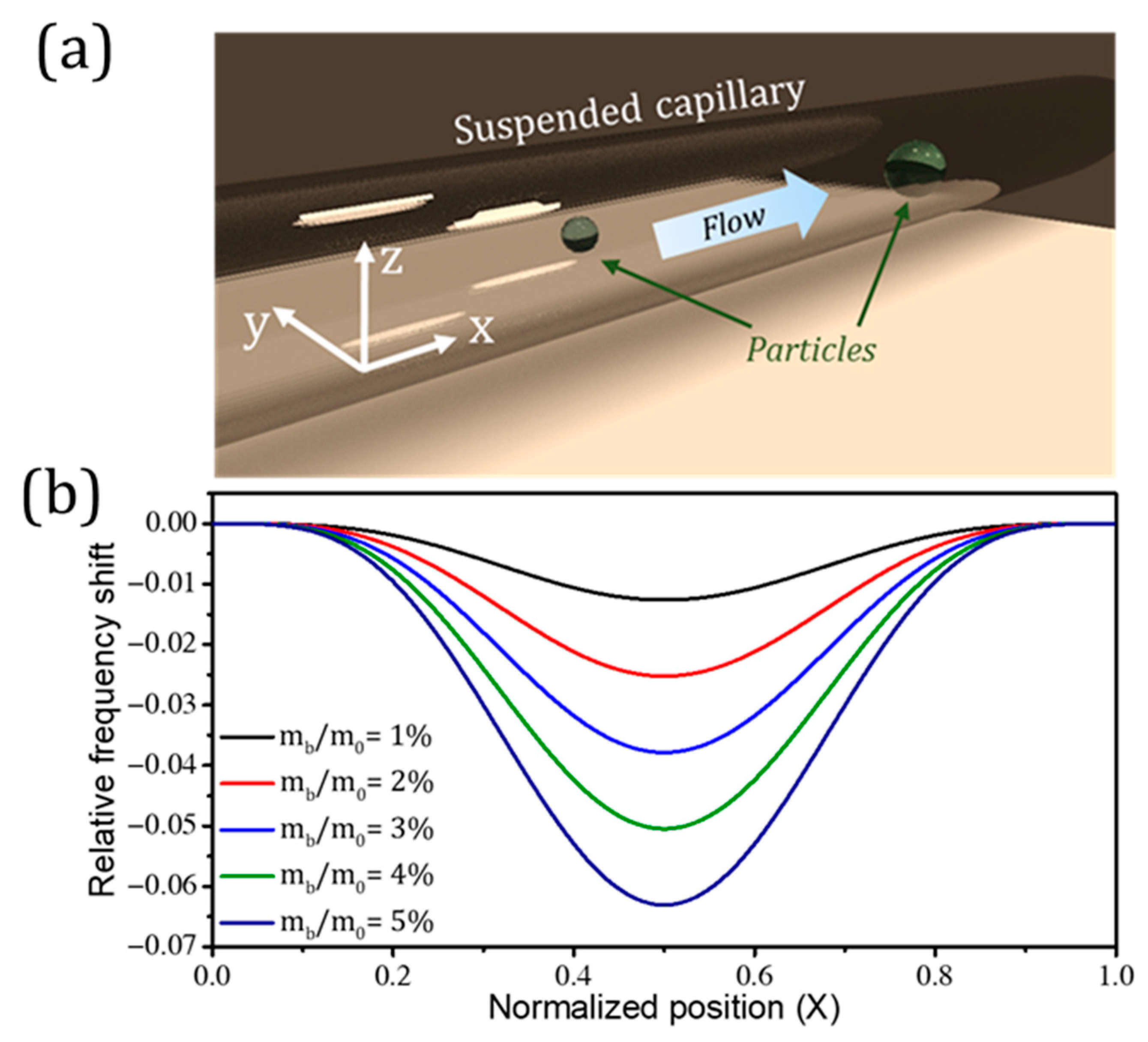
Recently, transparent hollow capillary resonators have been introduced to solve this problem by adding a new source of information: the optical properties of the flowing analytes [105]. Using a laser beam, it is possible to optically probe the analytes while measuring the mechanical displacement of the resonator [56]. In this technique, an interferometric measurement is used: light bounces between the suspended capillary and the substrate underneath, which provides an extraordinary displacement sensitivity [106]. The phase difference between the light reflected by the vibrating suspended capillary and the substrate provides the needed intensity modulation in the recombined beam reaching a photodetector. This approach uses a doubly clamped suspended resonator (Figure 8a) instead of a single clamped cantilever-like structure. The laser is focused on the center of the suspended area, where the displacement amplitude is maximal. As the phase difference between the reflected beams is not exactly π/2, the light collected by the photodetector carries double-sided information; that is, a harmonic intensity modulation given by interference caused by the mechanical displacement of the resonator (named as AC signal) over a non-modulated signal, which is proportional to the device reflectivity (named as DC signal). When a particle flows through the capillary, the mechanical resonance frequency consequently decreases owing to the added mass as well as the reflectivity when passing through the illuminated area as a result of the light scattering. From the reflectivity change (DC signal), it is possible to calculate the particle optical absorption, which depends on the material properties. However, in order to calculate intensive parameters such as the particle mass density or the refractive index, it is necessary to measure the particle size. In order to calculate it, it is necessary to know the velocity of the analytes passing through the device. From the mechanical frequency shift (AC signal) as a function of time (Figure 8b), the velocity of the particle is calculated by dividing the length of the suspended area (fixed by the device design) by the time it takes to recover the original frequency. The particle size is subsequently obtained by analyzing the optical scattering signal (DC signal) as a function of time. Whenever the flowing particle is illuminated by the laser spot, its edges scatter light, which is measured as a reflectivity signal drop. Thus, the diameter of the particle is finally calculated as the measured velocity multiplied by the elapsed time between two consecutive scattering signal drops.

The concept of buoyant mass comes from the Archimedes’ principle: an object immersed in liquid experiences a force equal to the weight of the displaced fluid. Thus, the buoyant mass of a spherical particle is defined as [107]

$$m_b=V_a\left({\rho }_a-{\rho }_f\right)$$

(52)

Hence, attending to the particle material and dimensions, it is possible to have particles of different materials and dimensions with the same buoyant mass. The problem of the buoyant mass becomes even more dramatic in the case of disperse particle populations given that two populations of different particles may be mechanically undiscernible, despite having a different average buoyant mass in the case wherein both distributions overlap. As an analyte flows through the suspended area, it produces a frequency shift given by

$$\frac{\Delta f}{f_0}=-\frac{1}{2}\frac{m_b}{m_0}{\psi }_n{\left(X\right)}^2$$

(53)

where $m_0$ is the mass of the resonator filled with fluid and ${\psi }_n\left(X\right)$ is the mode shape of a doubly clamped beam given by Equation (23). For the data analysis, the dips in the frequency signal produced by flowing analytes can be fitted to the shape of the mode by assuming that particles maintain a constant velocity while passing through the suspended region. These fits not only allow obtaining the frequency shift, but also give the transit time for each particle, which allows for directly calculating the velocity of the particle.

Suspended microchannel resonators have also been proposed to measure the compressibility of the particles that flow through them. Biological particles may have a high compressibility contrast with respect to the surrounding fluid; therefore, accessing the compressibility of the particle can add very valuable information for subsequent identification and analysis. Using an opto-mechano-fluidic resonator, Bahl et al. managed to measure the compressibility of small particles based on the change in the frequency associated with radially symmetric mechanical breathing modes of the resonator as the particle passes through it [108]. The formula that they proposed for the relative frequency shift contains the inertial term due to the mass and a new term including compression effects of the particle:

$$\frac{\Delta f}{f_0}=-\frac{{\chi }_a-{\chi }_f}{2{\chi }_f}C-\frac{{\rho }_a-{\rho }_f}{2{\rho }_a}D$$

(54)

where $\chi$ is the compressibility and subscripts $a$ and $f$ refer to analyte and fluid, respectively. The coefficients $C$ and $D$ provide the sensitivity to the compressibility and density contrasts between the liquid flowing inside the channel and the solid particle, and are given by

$$C=\frac{W_{ap}}{W_{fp}-W_{wp}}$$

(55)

$$D=\frac{W_{ak}}{W_{fk}-W_{wk}}$$

(56)

where $W_{ap}$ and $W_{ak}$ are the acoustic potential and kinetic energies, respectively, in the fluid evaluated over the volume displaced by the particle. $W_{fp}$ and $W_{fk}$ are the acoustic potential and kinetic energies, respectively, in the fluid evaluated over the entire volume of the fluid, and $W_{wp}$ and $W_{wk}$ are the strain and kinetic energies, respectively, associated with the solid part of the resonator.

Their capability to simultaneously access the analytes’ buoyant mass and compressibility, together with their extremely high speed, which enables characterizing a larger amount of analytes in a shorter time, settles optomechanical capillaries as one of the most promising devices in the field. The combination of optical and mechanical sensing methods in channeled platforms will revolutionize not only biology, biomedicine, and clinical diagnosis fields, but also the food industry and environmental analysis. However, in order to achieve success in accessing more and more precise information about the analytes, experimentalists still require more accurate theoretical models.

5. Summary

Nanomechanical sensors are rapidly gaining more and more attention from researchers and have been proven to be extraordinarily useful tools to monitor biological processes and to detect and measure the fundamental properties of biological entities. The advancements and developments of these systems are possible thanks to theories that allow the interpretation and understanding of the experimental observations. In this review, we have explored the main theories and models that are the base of nanomechanical sensors and that are used on a daily basis by researchers all over the world regarding this field. We have approached the topic by separating nanomechanical sensors into two main groups: static and dynamic. For the nanomechanical sensors in static mode, we have presented the main theories regarding the effect of differential surface stress on the bending of a rectangular cantilever plate, starting from the well-known Stoney’s equation, the improved solution proposed by Sader et al., and the simplified averaged curvatures expressions obtained by Tamayo et al. The effect of surface stress can also modify the dynamic properties of the sensor, allowing for quantifying the stress by measuring changes in the resonance frequencies of the nanomechanical resonator. This effect has been covered as well in this review, where we have mentioned both the model to explain the effect of net surface stress on cantilevers and doubly clamped beams and the model to explain the effect of differential surface stress on cantilever beams. Other features of the biological systems that can produce a shift in the natural frequencies of nanomechanical resonators are the mass and the stiffness. When the biological system is attached to the resonator surface, the resonant frequencies of the sensor change as a result of two opposite effects: the added mass decreases the frequencies, while the stiffness effect increases the frequencies. We have presented the main theoretical models for the effect of the mass and stiffness of analytes on the resonant frequencies of nanomechanical resonators, where we have emphasized the difference between the adsorption of a complete layer and the adsorption of individual particles. While the relative frequency shift is the same for all flexural modes in the case of a complete layer, for the individual particles, the relative frequency shift is different for different modes because it depends on the adsorption position. This particularity led to the multimode measuring technique that consists of measuring the relative frequency shifts of different vibration modes simultaneously in order to extract the mass, stiffness, and adsorption position of the attached particle. This process is known as the inverse problem and is the base for nanomechanical mass spectrometry. Multimode measuring can also be used to obtain the size and shape of a particle that cannot be considered as a point-like particle. The formalism to do so is called inertial imaging and has also been included in this review. Finally, in the last part of the review, we focused the attention on the effects of hydrodynamic loading when the sensor is immersed in a viscous fluid. This part is especially important when the nanomechanical sensor is used for biological applications because water is the natural environment of biology. We reviewed the main theories and models that describe the effects of hydrodynamic loading on the frequency and quality factor of cantilevers, as well as the new microchannel resonators that overcome the degradation of the quality factor as a result of viscous damping for sensing applications in liquid environments. To conclude, we would like to emphasize that theory and modeling are fundamental for the development and advancements of nanomechanical sensors, as they not only allow for the understanding of the phenomena, but also help to optimize the devices for a particular application. It is then a must that researchers can keep advancing the existing models and creating new ones in order to keep up the growth of this fascinating field.

References

- Chien, M.-H.; Brameshuber, M.; Rossboth, B.K.; Schütz, G.J.; Schmid, S. Single-molecule optical absorption imaging by nanomechanical photothermal sensing. Proc. Natl. Acad. Sci. USA 2018, 115, 11150. [Google Scholar] [CrossRef] [Green Version]
- Garcia, R. Nanomechanical mapping of soft materials with the atomic force microscope: Methods, theory and applications. Chem. Soc. Rev. 2020, 49, 5850–5884. [Google Scholar] [CrossRef] [PubMed]
- Barson, M.S.J.; Peddibhotla, P.; Ovartchaiyapong, P.; Ganesan, K.; Taylor, R.L.; Gebert, M.; Mielens, Z.; Koslowski, B.; Simpson, D.A.; McGuinness, L.P.; et al. Nanomechanical Sensing Using Spins in Diamond. Nano Lett. 2017, 17, 1496–1503. [Google Scholar] [CrossRef] [PubMed] [Green Version]
- Rugar, D.; Budakian, R.; Mamin, H.J.; Chui, B.W. Single spin detection by magnetic resonance force microscopy. Nature 2004, 430, 329–332. [Google Scholar] [CrossRef]
- Chan, J.; Alegre, T.P.M.; Safavi-Naeini, A.H.; Hill, J.T.; Krause, A.; Gröblacher, S.; Aspelmeyer, M.; Painter, O. Laser cooling of a nanomechanical oscillator into its quantum ground state. Nature 2011, 478, 89–92. [Google Scholar] [CrossRef] [PubMed] [Green Version]
- O’Connell, A.D.; Hofheinz, M.; Ansmann, M.; Bialczak, R.C.; Lenander, M.; Lucero, E.; Neeley, M.; Sank, D.; Wang, H.; Weides, M. Quantum ground state and single-phonon control of a mechanical resonator. Nature 2010, 464, 697–703. [Google Scholar] [CrossRef]
- Arlett, J.L.; Myers, E.B.; Roukes, M.L. Comparative advantages of mechanical biosensors. Nat. Nanotechnol. 2011, 6, 203–215. [Google Scholar] [CrossRef] [Green Version]
- Kosaka, P.M.; Pini, V.; Ruz, J.J.; Da Silva, R.A.; González, M.U.; Ramos, D.; Calleja, M.; Tamayo, J. Detection of cancer biomarkers in serum using a hybrid mechanical and optoplasmonic nanosensor. Nat. Nanotechnol. 2014, 9, 1047. [Google Scholar] [CrossRef]
- Hanay, M.S.; Kelber, S.; Naik, A.K.; Chi, D.; Hentz, S.; Bullard, E.C.; Colinet, E.; Duraffourg, L.; Roukes, M.L. Single-protein nanomechanical mass spectrometry in real time. Nat. Nanotechnol. 2012, 7, 602. [Google Scholar] [CrossRef] [PubMed]
- Malvar, O.; Ruz, J.J.; Kosaka, P.M.; Domínguez, C.M.; Gil-Santos, E.; Calleja, M.; Tamayo, J. Mass and stiffness spectrometry of nanoparticles and whole intact bacteria by multimode nanomechanical resonators. Nat. Commun. 2016, 7, 1–8. [Google Scholar] [CrossRef] [PubMed]
- Domínguez, C.M.; Ramos, D.; Mendieta-Moreno, J.I.; Fierro, J.L.G.; Mendieta, J.; Tamayo, J.; Calleja, M. Effect of water-DNA interactions on elastic properties of DNA self-assembled monolayers. Sci. Rep. 2017, 7, 536. [Google Scholar] [CrossRef] [PubMed] [Green Version]
- Del Rey, M.; Silva, R.A.D.; Meneses, D.; Petri, D.F.S.; Tamayo, J.; Calleja, M.; Kosaka, P.M. Monitoring swelling and deswelling of thin polymer films by microcantilever sensors. Sens. Actuators B Chem. 2014, 204, 602–610. [Google Scholar] [CrossRef] [Green Version]
- Domínguez, C.M.; Kosaka, P.M.; Mokry, G.; Pini, V.; Malvar, O.; del Rey, M.; Ramos, D.; San Paulo, Á.; Tamayo, J.; Calleja, M. Hydration Induced Stress on DNA Monolayers Grafted on Microcantilevers. Langmuir 2014, 30, 10962–10969. [Google Scholar] [CrossRef] [PubMed] [Green Version]
- Mertens, J.; Rogero, C.; Calleja, M.; Ramos, D.; Martín-Gago, J.A.; Briones, C.; Tamayo, J. Label-free detection of DNA hybridization based on hydration-induced tension in nucleic acid films. Nat. Nanotechnol. 2008, 3, 301–307. [Google Scholar] [CrossRef] [Green Version]
- Yubero, M.L.; Kosaka, P.M.; San Paulo, Á.; Malumbres, M.; Calleja, M.; Tamayo, J. Effects of energy metabolism on the mechanical properties of breast cancer cells. Commun. Biol. 2020, 3, 590. [Google Scholar] [CrossRef]
- Ligler, F.S.; Taitt, C.R. Optical Biosensors: Today and Tomorrow; Elsevier: Amsterdam, The Nethrelands, 2011. [Google Scholar]
- Waggoner, P.S.; Craighead, H.G. Micro-and nanomechanical sensors for environmental, chemical, and biological detection. Lab A Chip 2007, 7, 1238–1255. [Google Scholar] [CrossRef]
- Binnig, G.; Quate, C.F.; Gerber, C. Atomic Force Microscope. Phys. Rev. Lett. 1986, 56, 930–933. [Google Scholar] [CrossRef] [Green Version]
- Binnig, G.; Rohrer, H. Scanning tunneling microscopy. Surf. Sci. 1983, 126, 236–244. [Google Scholar] [CrossRef]
- Binnig, G.; Rohrer, H.; Salvan, F.; Gerber, C.; Baro, A. Revisiting the 7 × 7 reconstruction of Si(111). Surf. Sci. 1985, 157, L373–L378. [Google Scholar] [CrossRef]
- Eom, K.; Park, H.S.; Yoon, D.S.; Kwon, T. Nanomechanical resonators and their applications in biological/chemical detection: Nanomechanics principles. Phys. Rep. 2011, 503, 115–163. [Google Scholar] [CrossRef] [Green Version]
- Leng, H.; Lin, Y. A MEMS/NEMS sensor for human skin temperature measurement. Smart Struct. Syst. 2011, 8, 53–67. [Google Scholar] [CrossRef]
- Liu, P.S.; Tse, H.-F. Implantable sensors for heart failure monitoring. J. Arrhythmia 2013, 29, 314–319. [Google Scholar] [CrossRef] [Green Version]
- Boisen, A.; Dohn, S.; Keller, S.S.; Schmid, S.; Tenje, M. Cantilever-like micromechanical sensors. Rep. Prog. Phys. 2011, 74, 036101. [Google Scholar] [CrossRef]
- Tamayo, J.; Kosaka, P.M.; Ruz, J.J.; San Paulo, Á.; Calleja, M. Biosensors based on nanomechanical systems. Chem. Soc. Rev. 2013, 42, 1287–1311. [Google Scholar] [CrossRef] [Green Version]
- Barnes, J.R.; Stephenson, R.J.; Welland, M.E.; Gerber, C.; Gimzewski, J.K. Photothermal spectroscopy with femtojoule sensitivity using a micromechanical device. Nature 1994, 372, 79–81. [Google Scholar] [CrossRef]
- Thundat, T.; Chen, G.Y.; Warmack, R.J.; Allison, D.P.; Wachter, E.A. Vapor Detection Using Resonating Microcantilevers. Anal. Chem. 1995, 67, 519–521. [Google Scholar] [CrossRef]
- Thundat, T.; Wachter, E.A.; Sharp, S.L.; Warmack, R.J. Detection of mercury vapor using resonating microcantilevers. Appl. Phys. Lett. 1995, 66, 1695–1697. [Google Scholar] [CrossRef]
- Fritz, J.; Baller, M.K.; Lang, H.P.; Rothuizen, H.; Vettiger, P.; Meyer, E.J.; Güntherodt, H.; Gerber, C.; Gimzewski, J.K. Translating Biomolecular Recognition into Nanomechanics. Science 2000, 288, 316. [Google Scholar] [CrossRef] [Green Version]
- Ramos, D.; Tamayo, J.; Mertens, J.; Calleja, M.; Zaballos, A. Origin of the response of nanomechanical resonators to bacteria adsorption. J. Appl. Phys. 2006, 100, 106105. [Google Scholar] [CrossRef] [Green Version]
- Tamayo, J.; Ramos, D.; Mertens, J.; Calleja, M. Effect of the adsorbate stiffness on the resonance response of microcantilever sensors. Appl. Phys. Lett. 2006, 89, 224104. [Google Scholar] [CrossRef]
- Dominguez-Medina, S.; Fostner, S.; Defoort, M.; Sansa, M.; Stark, A.-K.; Halim, M.A.; Vernhes, E.; Gely, M.; Jourdan, G.; Alava, T.; et al. Neutral mass spectrometry of virus capsids above 100 megadaltons with nanomechanical resonators. Science 2018, 362, 918. [Google Scholar] [CrossRef] [PubMed] [Green Version]
- Gil-Santos, E.; Ramos, D.; Martínez, J.; Fernández-Regúlez, M.; García, R.; San Paulo, Á.; Calleja, M.; Tamayo, J. Nanomechanical mass sensing and stiffness spectrometry based on two-dimensional vibrations of resonant nanowires. Nat. Nanotechnol. 2010, 5, 641. [Google Scholar] [CrossRef] [PubMed] [Green Version]
- Malvar, O.; Gil-Santos, E.; Ruz, J.; Ramos, D.; Pini, V.; Fernández-Regúlez, M.; Calleja, M.; Tamayo, J.; Paulo, A. Tapered silicon nanowires for enhanced nanomechanical sensing. Appl. Phys. Lett. 2013, 103. [Google Scholar] [CrossRef] [Green Version]
- Yen, Y.-K.; Chiu, C.-Y. A CMOS MEMS-based Membrane-Bridge Nanomechanical Sensor for Small Molecule Detection. Sci. Rep. 2020, 10, 2931. [Google Scholar] [CrossRef] [PubMed]
- Burg, T.P.; Manalis, S.R. Suspended microchannel resonators for biomolecular detection. Appl. Phys. Lett. 2003, 83, 2698–2700. [Google Scholar] [CrossRef] [Green Version]
- Godin, M.; Bryan, A.K.; Burg, T.P.; Babcock, K.; Manalis, S.R. Measuring the mass, density, and size of particles and cells using a suspended microchannel resonator. Appl. Phys. Lett. 2007, 91, 123121. [Google Scholar] [CrossRef] [Green Version]
- Malvar, O.; Ramos, D.; Martínez, C.; Kosaka, P.; Tamayo, J.; Calleja, M. Highly sensitive measurement of liquid density in air using suspended microcapillary resonators. Sensors 2015, 15, 7650–7657. [Google Scholar] [CrossRef]
- Lee, I.; Park, K.; Lee, J. Note: Precision viscosity measurement using suspended microchannel resonators. Rev. Sci. Instrum. 2012, 83, 116106. [Google Scholar] [CrossRef]
- Linden, J.; Thyssen, A.; Oesterschulze, E. Suspended plate microresonators with high quality factor for the operation in liquids. Appl. Phys. Lett. 2014, 104, 191906. [Google Scholar] [CrossRef]
- Dohn, S.; Sandberg, R.; Svendsen, W.; Boisen, A. Enhanced functionality of cantilever based mass sensors using higher modes. Appl. Phys. Lett. 2005, 86, 233501. [Google Scholar] [CrossRef] [Green Version]
- Xu, W.; Choi, S.; Chae, J. A contour-mode film bulk acoustic resonator of high quality factor in a liquid environment for biosensing applications. Appl. Phys. Lett. 2010, 96, 053703. [Google Scholar] [CrossRef] [Green Version]
- Ramos, D.; Mertens, J.; Calleja, M.; Tamayo, J. Phototermal self-excitation of nanomechanical resonators in liquids. Appl. Phys. Lett. 2008, 92, 173108. [Google Scholar] [CrossRef]
- Burg, T.P.; Godin, M.; Knudsen, S.M.; Shen, W.; Carlson, G.; Foster, J.S.; Babcock, K.; Manalis, S.R. Weighing of biomolecules, single cells and single nanoparticles in fluid. Nature 2007, 446, 1066–1069. [Google Scholar] [CrossRef] [PubMed] [Green Version]
- Favero, I.; Karrai, K. Optomechanics of deformable optical cavities. Nat. Photonics 2009, 3, 201–205. [Google Scholar] [CrossRef]
- Fong, K.Y.; Poot, M.; Tang, H.X. Nano-Optomechanical Resonators in Microfluidics. Nano Lett. 2015, 15, 6116–6120. [Google Scholar] [CrossRef] [Green Version]
- Gil-Santos, E.; Baker, C.; Nguyen, D.T.; Hease, W.; Gomez, C.; Lemaître, A.; Ducci, S.; Leo, G.; Favero, I. High-frequency nano-optomechanical disk resonators in liquids. Nat. Nanotechnol. 2015, 10, 810. [Google Scholar] [CrossRef]
- Gil-Santos, E.; Ramos, D.; Pini, V.; Llorens, J.; Fernandez-Regulez, M.; Calleja, M.; Tamayo, J.; San Paulo, A. Optical back-action in silicon nanowire resonators: Bolometric versus radiation pressure effects. New J. Phys. 2013, 15. [Google Scholar] [CrossRef] [Green Version]
- Gil-Santos, E.; Ruz, J.J.; Malvar, O.; Favero, I.; Lemaître, A.; Kosaka, P.M.; García-López, S.; Calleja, M.; Tamayo, J. Optomechanical detection of vibration modes of a single bacterium. Nat. Nanotechnol. 2020, 15, 469–474. [Google Scholar] [CrossRef]
- Kosaka, P.M.; Calleja, M.; Tamayo, J. Optomechanical devices for deep plasma cancer proteomics. Semin. Cancer Biol. 2018, 52, 26–38. [Google Scholar] [CrossRef]
- Zhang, H.; Xj, Z.; Wang, Y.; Huang, Q.; Xia, J. Femtogram scale high frequency nano-optomechanical resonators in water. Opt. Express 2017, 25, 821. [Google Scholar] [CrossRef]
- Cleland, A.N.; Roukes, M.L. Noise processes in nanomechanical resonators. J. Appl. Phys. 2002, 92, 2758–2769. [Google Scholar] [CrossRef] [Green Version]
- Stoney, G.G. The tension of metallic films deposited by electrolysis. Proc. R. Soc. Lond. Ser. A Contain. Pap. A Math. Phys. Character 1909, 82, 172–175. [Google Scholar]
- Gruber, K.; Horlacher, T.; Castelli, R.; Mader, A.; Seeberger, P.H.; Hermann, B.A. Cantilever Array Sensors Detect Specific Carbohydrate−Protein Interactions with Picomolar Sensitivity. ACS Nano 2011, 5, 3670–3678. [Google Scholar] [CrossRef] [PubMed]
- Mader, A.; Gruber, K.; Castelli, R.; Hermann, B.A.; Seeberger, P.H.; Rädler, J.O.; Leisner, M. Discrimination of Escherichia coli Strains using Glycan Cantilever Array Sensors. Nano Lett. 2012, 12, 420–423. [Google Scholar] [CrossRef]
- McKendry, R.; Zhang, J.; Arntz, Y.; Strunz, T.; Hegner, M.; Lang, H.P.; Baller, M.K.; Certa, U.; Meyer, E.; Güntherodt, H.-J.; et al. Multiple label-free biodetection and quantitative DNA-binding assays on a nanomechanical cantilever array. Proc. Natl. Acad. Sci. USA 2002, 99, 9783. [Google Scholar] [CrossRef] [Green Version]
- Sader, J.E. Surface stress induced deflections of cantilever plates with applications to the atomic force microscope: Rectangular plates. J. Appl. Phys. 2001, 89, 2911–2921. [Google Scholar] [CrossRef] [Green Version]
- Tamayo, J.; Ruz, J.J.; Pini, V.; Kosaka, P.; Calleja, M. Quantification of the surface stress in microcantilever biosensors: Revisiting Stoney’s equation. Nanotechnology 2012, 23, 475702. [Google Scholar] [CrossRef] [Green Version]
- Thundat, P.I.O.; Warmack, R.J. MICROCANTILEVER SENSORS. Microscale Eng. 1997, 1, 185–199. [Google Scholar] [CrossRef]
- Ilic, B.; Czaplewski, D.; Craighead, H.G.; Neuzil, P.; Campagnolo, C.; Batt, C. Mechanical resonant immunospecific biological detector. Appl. Phys. Lett. 2000, 77, 450–452. [Google Scholar] [CrossRef]
- Ruz, J.J.; Tamayo, J.; Pini, V.; Kosaka, P.M.; Calleja, M. Physics of nanomechanical spectrometry of viruses. Sci. Rep. 2014, 4, 1–11. [Google Scholar] [CrossRef] [Green Version]
- Ruz, J.J.; Malvar, O.; Gil-Santos, E.; Calleja, M.; Tamayo, J. Effect of particle adsorption on the eigenfrequencies of nano-mechanical resonators. J. Appl. Phys. 2020, 128, 104503. [Google Scholar] [CrossRef]
- Ramos, D.; Mertens, J.; Calleja, M.; Tamayo, J. Study of the origin of bending induced by bimetallic effect on microcantilever. Sensors 2007, 7, 1757. [Google Scholar] [CrossRef] [PubMed] [Green Version]
- Ramos, D.; Tamayo, J.; Mertens, J.; Calleja, M. Photothermal excitation of microcantilevers in liquids. J. Appl. Phys. 2006, 99, 124904. [Google Scholar] [CrossRef] [Green Version]
- Toda, M.; Inomata, N.; Ono, T.; Voiculescu, I. Cantilever beam temperature sensors for biological applications. IEEJ Trans. Electr. Electron. Eng. 2017, 12, 153–160. [Google Scholar] [CrossRef] [Green Version]
- Wu, L.; Cheng, T.; Zhang, Q.-C. A bi-material microcantilever temperature sensor based on optical readout. Measurement 2012, 45, 1801–1806. [Google Scholar] [CrossRef]
- Kang, K.; Nilsen-Hamilton, M.; Shrotriya, P. Differential surface stress sensor for detection of chemical and biological species. Appl. Phys. Lett. 2008, 93, 143107. [Google Scholar] [CrossRef] [Green Version]
- Sang, S.; Zhao, Y.; Zhang, W.; Li, P.; Hu, J.; Li, G. Surface stress-based biosensors. Biosens. Bioelectron. 2014, 51, 124–135. [Google Scholar] [CrossRef]
- Godin, M.; Tabard-Cossa, V.; Miyahara, Y.; Monga, T.; Williams, P.J.; Beaulieu, L.Y.; Lennox, R.B.; Grutter, P. Cantilever-based sensing: The origin of surface stress and optimization strategies. Nanotechnology 2010, 21, 075501. [Google Scholar] [CrossRef]
- Haiss, W. Surface stress of clean and adsorbate-covered solids. Rep. Prog. Phys. 2001, 64, 591–648. [Google Scholar] [CrossRef]
- Ibach, H. Adsorbate-induced surface stress. J. Vac. Sci. Technol. A Vac. Surf. Film. 1994, 12, 2240–2245. [Google Scholar] [CrossRef]
- Timoshenko, S.; Woinowsky-Krieger, S. Theory of Plates and Shells; McGraw-Hill: New York, NY, USA, 1959. [Google Scholar]
- Zeng, X.; Deng, J.; Luo, X. Deflection of a cantilever rectangular plate induced by surface stress with applications to surface stress measurement. J. Appl. Phys. 2012, 111, 083531. [Google Scholar] [CrossRef]
- Timoshenko, S.P. Theory of Elasticity; McGraw-Hill Education (India) Pvt Limited: Noida, India, 2010. [Google Scholar]
- Ziegler, C. Cantilever-based biosensors. Anal. Bioanal. Chem. 2004, 379, 946–959. [Google Scholar] [CrossRef] [PubMed]
- Karabalin, R.B.; Villanueva, L.G.; Matheny, M.H.; Sader, J.E.; Roukes, M.L. Stress-induced variations in the stiffness of micro-and nanocantilever beams. Phys. Rev. Lett. 2012, 108, 236101. [Google Scholar] [CrossRef] [PubMed] [Green Version]
- Lachut, M.J.; Sader, J.E. Effect of surface stress on the stiffness of thin elastic plates and beams. Phys. Rev. B 2012, 85, 085440. [Google Scholar] [CrossRef] [Green Version]
- Chen, G.Y.; Thundat, T.; Wachter, E.A.; Warmack, R.J. Adsorption-induced surface stress and its effects on resonance frequency of microcantilevers. J. Appl. Phys. 1995, 77, 3618–3622. [Google Scholar] [CrossRef]
- Gurtin, M.E.; Markenscoff, X.; Thurston, R.N. Effect of surface stress on the natural frequency of thin crystals. Appl. Phys. Lett. 1976, 29, 529–530. [Google Scholar] [CrossRef]
- Lagowski, J.; Gatos, H.C.; Sproles, E.S. Surface stress and the normal mode of vibration of thin crystals:GaAs. Appl. Phys. Lett. 1975, 26, 493–495. [Google Scholar] [CrossRef]
- Lu, P.; Lee, H.P.; Lu, C.; O’shea, S.J. Surface stress effects on the resonance properties of cantilever sensors. Phys. Rev. B 2005, 72, 085405. [Google Scholar] [CrossRef]
- Pini, V.; Tamayo, J.; Gil-Santos, E.; Ramos, D.; Kosaka, P.; Tong, H.-D.; van Rijn, C.; Calleja, M. Shedding Light on Axial Stress Effect on Resonance Frequencies of Nanocantilevers. ACS Nano 2011, 5, 4269–4275. [Google Scholar] [CrossRef] [Green Version]
- Lachut, M.J.; Sader, J.E. Effect of surface stress on the stiffness of cantilever plates. Phys. Rev. Lett. 2007, 99, 206102. [Google Scholar] [CrossRef]
- Pini, V.; Ruz, J.; Kosaka, P.; Malvar, O.; Calleja, M.; Tamayo, J. How two-dimensional bending can extraordinarily stiffen thin sheets. Sci. Rep. 2016, 6. [Google Scholar] [CrossRef] [PubMed] [Green Version]
- Ruz, J.J.; Pini, V.; Malvar, O.; Kosaka, P.M.; Calleja, M.; Tamayo, J. Effect of surface stress induced curvature on the eigenfrequencies of microcantilever plates. AIP Adv. 2018, 8, 105213. [Google Scholar] [CrossRef]
- Ramos, D.; Tamayo, J.; Mertens, J.; Calleja, M.; Villanueva, L.G.; Zaballos, A. Detection of bacteria based on the thermomechanical noise of a nanomechanical resonator: Origin of the response and detection limits. Nanotechnology 2007, 19, 035503. [Google Scholar] [CrossRef] [PubMed]
- Hanay, M.S.; Kelber, S.I.; O’Connell, C.D.; Mulvaney, P.; Sader, J.E.; Roukes, M.L. Inertial imaging with nanomechanical systems. Nat. Nanotechnol. 2015, 10, 339–344. [Google Scholar] [CrossRef] [PubMed]
- Naik, A.K.; Hanay, M.S.; Hiebert, W.K.; Feng, X.L.; Roukes, M.L. Towards single-molecule nanomechanical mass spectrometry. Nat. Nanotechnol. 2009, 4, 445–450. [Google Scholar] [CrossRef] [PubMed]
- Ramos, D.; Malvar, O.; Davis, Z.J.; Tamayo, J.; Calleja, M. Nanomechanical Plasmon Spectroscopy of Single Gold Nanoparticles. Nano Lett. 2018, 18, 7165–7170. [Google Scholar] [CrossRef]
- Sage, E.; Brenac, A.; Alava, T.; Morel, R.; Dupré, C.; Hanay, M.S.; Roukes, M.L.; Duraffourg, L.; Masselon, C.; Hentz, S. Neutral particle mass spectrometry with nanomechanical systems. Nat. Commun. 2015, 6, 1–5. [Google Scholar] [CrossRef] [Green Version]
- Ekinci, K.L.; Roukes, M.L. Nanoelectromechanical systems. Rev. Sci. Instrum. 2005, 76, 061101. [Google Scholar] [CrossRef] [Green Version]
- Sansa, M.; Sage, E.; Bullard, E.C.; Gély, M.; Alava, T.; Colinet, E.; Naik, A.K.; Villanueva, L.G.; Duraffourg, L.; Roukes, M.L.; et al. Frequency fluctuations in silicon nanoresonators. Nat. Nanotechnol. 2016, 11, 552–558. [Google Scholar] [CrossRef] [Green Version]
- Kiracofe, D.; Raman, A. On eigenmodes, stiffness, and sensitivity of atomic force microscope cantilevers in air versus liquids. J. Appl. Phys. 2010, 107, 033506. [Google Scholar] [CrossRef] [Green Version]
- Lee, J.W.; Tung, R.; Raman, A.; Sumali, H.; Sullivan, J.P. Squeeze-film damping of flexible microcantilevers at low ambient pressures: Theory and experiment. J. Micromech. Microeng. 2009, 19, 105029. [Google Scholar] [CrossRef]
- Ricci, A.; Canavese, G.; Ferrante, I.; Marasso, S.L.; Ricciardi, C. A finite element model for the frequency spectrum estimation of a resonating microplate in a microfluidic chamber. Microfluid. Nanofluid. 2013, 15, 275–284. [Google Scholar] [CrossRef]
- Ricciardi, C.; Canavese, G.; Castagna, R.; Ferrante, I.; Ricci, A.; Marasso, S.L.; Napione, L.; Bussolino, F. Integration of microfluidic and cantilever technology for biosensing application in liquid environment. Biosens. Bioelectron. 2010, 26, 1565–1570. [Google Scholar] [CrossRef] [PubMed]
- Papi, M.; Arcovito, G.; De Spirito, M.; Vassalli, M.; Tiribilli, B. Fluid viscosity determination by means of uncalibrated atomic force microscopy cantilevers. Appl. Phys. Lett. 2006, 88, 194102. [Google Scholar] [CrossRef] [Green Version]
- Paul, M.R.; Clark, M.T.; Cross, M.C. The stochastic dynamics of micron and nanoscale elastic cantilevers in fluid: Fluctuations from dissipation. Nanotechnology 2006, 17, 4502–4513. [Google Scholar] [CrossRef]
- Sader, J.E. Frequency response of cantilever beams immersed in viscous fluids with applications to the atomic force microscope. J. Appl. Phys. 1998, 84, 64–76. [Google Scholar] [CrossRef] [Green Version]
- Van Eysden, C.A.; Sader, J.E. Frequency response of cantilever beams immersed in viscous fluids with applications to the atomic force microscope: Arbitrary mode order. J. Appl. Phys. 2007, 101, 044908. [Google Scholar] [CrossRef]
- Maali, A.; Hurth, C.; Boisgard, R.; Jai, C.; Cohen-Bouhacina, T.; Aimé, J.-P. Hydrodynamics of oscillating atomic force microscopy cantilevers in viscous fluids. J. Appl. Phys. 2005, 97, 074907. [Google Scholar] [CrossRef]
- Son, S.; Tzur, A.; Weng, Y.; Jorgensen, P.; Kim, J.; Kirschner, M.W.; Manalis, S.R. Direct observation of mammalian cell growth and size regulation. Nat. Methods 2012, 9, 910–912. [Google Scholar] [CrossRef] [Green Version]
- Martín-Pérez, A.; Ramos, D.; Tamayo, J.; Calleja, M. Real-Time Particle Spectrometry in Liquid Environment Using Microfluidic-Nanomechanical Resonators. In Proceedings of the 2019 20th International Conference on Solid-State Sensors, Actuators and Microsystems & Eurosensors XXXIII (TRANSDUCERS & EUROSENSORS XXXIII), Berlin, Germany, 23–27 June 2019; pp. 2146–2149. [Google Scholar]
- Olcum, S.; Cermak, N.; Wasserman, S.C.; Christine, K.S.; Atsumi, H.; Payer, K.R.; Shen, W.; Lee, J.; Belcher, A.M.; Bhatia, S.N.; et al. Weighing nanoparticles in solution at the attogram scale. Proc. Natl. Acad. Sci. USA 2014, 111, 1310. [Google Scholar] [CrossRef] [Green Version]
- Martín-Pérez, A.; Ramos, D.; Tamayo, J.; Calleja, M. Coherent Optical Transduction of Suspended Microcapillary Resonators for Multi-Parameter Sensing Applications. Sensors 2019, 19, 5069. [Google Scholar] [CrossRef] [PubMed] [Green Version]
- Pini, V.; Ramos, D.; Domínguez, C.M.; Ruz, J.; Malvar, O.; Kosaka, P.; Davis, Z.; Tamayo, J.; Calleja, M. Optimization of the readout of microdrum optomechanical resonators. Microelectron. Eng. 2017, 183, 37–41. [Google Scholar] [CrossRef]
- Martín-Pérez, A.; Ramos, D.; Gil-Santos, E.; García-López, S.; Yubero, M.L.; Kosaka, P.M.; San Paulo, Á.; Tamayo, J.; Calleja, M. Mechano-Optical Analysis of Single Cells with Transparent Microcapillary Resonators. ACS Sens. 2019, 4, 3325–3332. [Google Scholar] [CrossRef] [PubMed]
- Han, K.; Suh, J.; Bahl, G. Optomechanical non-contact measurement of microparticle compressibility in liquids. Opt. Express 2018, 26, 31908–31916. [Google Scholar] [CrossRef]
Figure 1.
(a) Schematic depiction of the two different operation modes, static and dynamic, in which a nanomechanical sensor can function, showing their basic principle of operation when used for biological applications. (b) Chronogram of the publication and citation rate in the nanomechanical sensing field, focused on biological applications, and splitting them into static (red) and dynamic (black) operation modes.
Figure 2.
(a) Schematic of a cantilever plate that has been bent by the action of differential surface stress between the upper and lower faces. (b) Contour lines of the longitudinal and transversal curvatures normalized to Stoney’s curvature for a cantilever plate. It can be seen that, far from the clamped region, both curvatures follow Stoney’s equation, which is not the case for the region close to the clamping.
Figure 3.
(a) Theoretical prediction of the relative frequency shift due to net surface stress for the fundamental mode of a silicon nitride cantilever of 100 nm in thickness and 20 µm in length for different values of the width. (b–d) The theoretical prediction of the relative frequency shift due to the differential surface stress for the same cantilever and for the first, second, and third flexural modes, respectively, as well as for different values of the width. Insets show a representation of the mode shape.
Figure 4.
(a) Influence of the adsorbed layer on the flexural modes of a silicon beam as a function of the ratio between thicknesses and for different values of the Young’s modulus of the adsorbed material. (b) Same graph, but at the range of values of where the linear approximation (21) can be applied.
Figure 5.
(a) Schematic depiction of a bacterium adsorbed longitudinally and transversally oriented on a resonator. (b,c) Relative frequency shift produced by the adsorption of a typical E. coli bacterium on a silicon nitride cantilever and a doubly clamped beam of 200 × 20 × 0.6 µm for the first three flexural modes. It can be seen that, because of the edge effects of the bacterium, the stiffness effect is considerably smaller when the bacterium is transversally oriented.
Figure 6.
Schematic of the particle’s mass and stiffness determination using multimode measuring. In a first step, the frequencies of the resonator are tracked and the relative frequency shifts produced by the particle adsorption are recorded. In a second step, the joint probability density function () is formed using the frequency noise for each of the modes being tracked. Finally, the can be integrated in the normalized position and either in or to obtain the mass or the stiffness , respectively.
Figure 7.
(a) Real (solid line) and imaginary (dashed line) parts of the hydrodynamic function as a function of the oscillation frequency for a rectangular cantilever of 200 μm in length and 20 μm in width immersed in water. (b) Theoretical simulation of amplitude spectra of two equivalent nanomechanical resonators: one oscillating in vacuum (solid line) and one oscillating in liquid (dashed line). The effective mass and damping constant of the resonator in vacuum were consequently changed to obtain an equivalent liquid immersed resonator.
Figure 8.
(a) Schematic depiction of a hollow transparent suspended capillary with flowing particles inside. (b) Theoretical prediction of the relative frequency shift for the first mode of the capillary for different masses as a function of the position.
Publisher’s Note: MDPI stays neutral with regard to jurisdictional claims in published maps and institutional affiliations. |
© 2021 by the authors. Licensee MDPI, Basel, Switzerland. This article is an open access article distributed under the terms and conditions of the Creative Commons Attribution (CC BY) license (http://creativecommons.org/licenses/by/4.0/).
Share and Cite
MDPI and ACS Style
Ruz, J.J.; Malvar, O.; Gil-Santos, E.; Ramos, D.; Calleja, M.; Tamayo, J. A Review on Theory and Modelling of Nanomechanical Sensors for Biological Applications. Processes 2021, 9, 164. https://0-doi-org.brum.beds.ac.uk/10.3390/pr9010164
AMA Style
Ruz JJ, Malvar O, Gil-Santos E, Ramos D, Calleja M, Tamayo J. A Review on Theory and Modelling of Nanomechanical Sensors for Biological Applications. Processes. 2021; 9(1):164. https://0-doi-org.brum.beds.ac.uk/10.3390/pr9010164
Chicago/Turabian StyleRuz, Jose Jaime, Oscar Malvar, Eduardo Gil-Santos, Daniel Ramos, Montserrat Calleja, and Javier Tamayo. 2021. "A Review on Theory and Modelling of Nanomechanical Sensors for Biological Applications" Processes 9, no. 1: 164. https://0-doi-org.brum.beds.ac.uk/10.3390/pr9010164
Note that from the first issue of 2016, this journal uses article numbers instead of page numbers. See further details here.