Numerical Study on Unsteady Pressure Distribution on Bulk Carrier in Head Waves with Forward Speed

Abstract

This study deals with wave-induced unsteady pressure on a ship moving with a constant forward speed in regular head waves. Two different numerical methods are applied to solve wave–ship interaction problems: a Rankine panel method which adopts velocity potential, and a Cartesian-grid method which solves the momentum and mass conservation equations under the assumption of inviscid and incompressible fluids. Before comparing l1ocal pressure distributions, the computational methods are validated for global quantities, such as ship motion responses and added resistance, by comparison with available experimental data. Then, the computational results and experimental data are compared for hydrodynamic pressure, particularly focusing on the magnitude of the first-harmonic component in different sections and vertical locations. Furthermore, the Cartesian-grid method is used to simulate the various wave-amplitude conditions, and the characteristics of the zeroth-, first-, and second-harmonic components of wave-induced pressure are investigated. The nonlinearity of pressure distribution is observed mostly from the pressure near the still-water-level of the ship bow and the normalized first-harmonic component of wave-induced pressure decreases as the wave steepness increases. Lastly, to understand the local characteristics of wave-induced unsteady pressure, the time-averaged added pressure and added local force are analyzed. It is found that the major contribution of the time-averaged added local force that occurs around the ship stem above the design waterline.

1. Introduction

An estimation of seakeeping performances is one of the important procedures in safe ship design. Thanks to rapid progress in computing power, many numerical methods, such as potential flow solvers and computational fluid dynamics (CFD), have been applied to estimate a ship’s behavior in various environmental conditions [1,2,3]. In addition to motion responses, the added resistance of a ship due to waves also becomes an important topic to estimate a ship’s performance in waves [4,5,6,7,8]. However, those quantities are global or integrated values, rather than local or primitive physical values. Thus, the validation of local physical variables is essential to establish reliable numerical methods for the prediction of ship performance in waves. Furthermore, based on the observation of local flows, physical understanding of the flow around a ship in waves can be deepened, and numerical methods can be improved.

In an experiment, it is relatively easy to measure hydrodynamic forces acting on a ship by a dynamometer, whereas the measurement of local variables, such as hydrodynamic pressure and velocity distribution around a ship, requires laborious work. Tanizawa et al. [9] conducted an experimental study of a very large crude carrier (VLCC) model ship in various wave headings and wavelengths with 15 strain-gage type pressure sensors, and Kashiwagi et al. [10] compared the experimental data of pressure with the enhanced unified theory (EUT). Chiu et al. [11] carried out a series of experiments for a high-speed vessel in regular head waves with 25 strain-gage type pressure sensors, and proposed an algorithm for finding frequency response functions in third-order Volterra models, to simulate the variation of pressure responses in regular waves. Tiao [12] conducted further investigations for irregular waves.

Recently, Iwashita et al. [13] compared the unsteady pressure distribution on the Research Initiative on Oceangoing Ships (RIOS) bulk carrier in head sea condition between Rankine panel method (RPM) and experiment, and Iwashita and Kashiwagi [14] conducted further systematic experimental studies. In the experiment, more than 230 Fiber Bragg Gratings (FBG) sensors were attached on the starboard side of the ship hull and ordinary pressure sensors of strain-gage type were installed in the port side of the ship. The corresponding results were also computed by RPM and EUT, and the distribution of added pressure was extracted from the measured data to investigate the added resistance due to waves in more detail.

Orihara et al. [15] conducted a numerical study about the added resistance in waves and studied the characteristics of time-averaged pressure on the ship surface for different bow shapes using a CFD code Wave vIScous flow Difference Accurate Method-X (WISDAM-X). Sadat-Hosseini et al. [16] also studied the added resistance in waves, experimentally and numerically, and they showed the distribution of harmonic force components on the ship for different wavelengths. They concluded that high pressure acting on the upper bow is a major contribution to the added resistance, and the size of the high-pressure region correlates with the bow relative motion. Recently, Yang and Kim [17] investigated the distribution pattern of time-averaged added pressure in short waves using a Cartesian-grid method. The effects of wave steepness were also investigated and one of the findings in that study is that the time-averaged added pressure shows a similar distribution shape even for different wave steepness.

Many studies compared unsteady pressure at a few points on the ship surface or only provided numerical results of pressure distribution. In the present work, the characteristics of wave-induced unsteady pressure, which is one of the primitive physical values in hydrodynamics, on whole ship surface is studied by experimentally and numerically including fully nonlinear computations. To solve wave–ship interaction problems, two different numerical methods are applied. The first one is a Rankine panel method, which is based on potential flows and linearized free-surface boundary value problems. The other one is a Cartesian-grid method that can simulate highly nonlinear free-surface flows. Before comparing local pressure distribution, global quantities—ship motion responses and added resistance due to waves—are validated with experimental data. Then, comparisons between computational results and experimental data have been made for the magnitude of the first-harmonic component of wave-induced pressure on different sections and various vertical locations. In addition to the small steepness wave case, different amplitudes of incident wave are studied using the Cartesian-grid method, and the characteristics of the zeroth-, first-, and second-harmonic components of wave-induced pressure have been examined. Finally, the time-averaged added pressure and added local force have been investigated, to understand the physical characteristics of added resistance of a ship in head waves.

2. Mathematical Backgrounds

2.1. Cartesian-Grid Method

Air, water, and solid phases are considered to solve ship motion problems in the present Cartesian-grid method, called Seoul National University-Marine Hydrodynamics Laboratory-Computational Fluid Dynamics, or SNU-MHL-CFD, ver. 2.0. The details of the Cartesian-grid method can be found in Yang and Kim [17], and the numerical procedure is briefly summarized here.

The right-handed coordinate system which is moving with the constant forward speed U of the ship is introduced and the origin is located at the center of gravity of the ship. The x-axis is parallel to the ship’s longitudinal direction pointing to the ship stern and the starboard side of the ship is the positive y-axis. The z-axis is normal to the other two axes, that means positive upward. Many wave–ship interaction problems are dominated by the inertia effect. Thus, the fluid viscosity can be ignored, and the following continuity and Euler equations are solved:

$$\nabla \cdot \overrightarrow{u}=0,$$

(1)

$$\frac{\partial \overrightarrow{u}}{\partial t}+\overrightarrow{u}\cdot \nabla \overrightarrow{u}=-\frac{1}{\rho }\nabla p+\overrightarrow{b}$$

(2)

where $\overrightarrow{u}$ is the velocity vector, ρ means the fluid density, p is the pressure, and b is the body-force vector. A fractional-step method is applied for velocity and pressure coupling and the finite-volume method with staggered variable allocation is used for the spatial discretization. The pressure Poisson equation is solved using a multi-grid algorithm to update the pressure in the fluid domain:

$$\nabla \cdot \left(\frac{1}{\rho }\nabla p\right)=\frac{1}{\Delta t}\nabla \cdot \overrightarrow{u}$$

(3)

where ∆t means the time step. The hydrostatic pressure was eliminated for the ship part that was initially submerged in the water, when calculating the time history of pressure. Thus, the pressure in the subsequent section includes both linear and nonlinear hydrodynamic pressure, and hydrostatic pressure above the still water level.

An immersed boundary method is used and the volume fraction of each phase in each cell is calculated [18]. The tangent of hyperbola for interface capturing (THINC) and weighted line interface calculation (WLIC) methods [19,20] are applied to update the volume-fraction function of the water phase. In this formulation, incompressible fluid is assumed for both air and water phases and the free surface boundary conditions are implicitly satisfied. The volume fraction of a solid body is calculated by the transformation of a signed distance field between the ship surface and a grid point. The slip boundary condition is satisfied by a volume-weighted formula [17,21]:

$$\widehat{\overrightarrow{u}}=\{\begin{array}{l}\left(1-{\alpha }_3^{\overrightarrow{u}}\right)\overrightarrow{u}+{\alpha }_3^{\overrightarrow{u}}{\overrightarrow{U}}_{body} \hspace{1em}\hspace{1em}\hspace{1em}\hspace{1em}\hspace{1em}\hspace{0.17em}\hspace{0.17em}\hspace{0.17em}\hspace{0.17em}\hspace{0.17em}\hspace{0.17em}\hspace{0.17em}\hspace{0.17em}\hspace{0.17em}\hspace{0.17em}\mathrm{if}\hspace{0.17em}\hspace{0.17em}{\alpha }_3^{\overrightarrow{u}}\ge 0.5\\ \left[\left(1-{\alpha }_3^{\overrightarrow{u}}\right)N\overrightarrow{u}+{\alpha }_3^{\overrightarrow{u}}N{\overrightarrow{U}}_{body}\right]+\left(I-N\right)\overrightarrow{u}\hspace{0.17em}\hspace{0.17em}\hspace{0.17em}\hspace{0.17em}\mathrm{if}\hspace{0.17em}\hspace{0.17em}{\alpha }_3^{\overrightarrow{u}}<0.5\end{array}$$

(4)

where $\widehat{\overrightarrow{u}}$ indicates the updated fluid velocity, ${\overrightarrow{U}}_{body}$ is the velocity of ship surface closest to the center of velocity-control volume, ${\alpha }_3^{\overrightarrow{u}}$ is the volume fraction of the ship in the corresponding velocity-control volume, I is the identity matrix, and N is the normal dyad.

To generate the incident waves and eliminate reflecting waves from the ship, forcing terms are added in the momentum conservation equations. The forcing term is calculated using the difference between numerical solutions and Stokes analytic solutions of fluid velocities and wave elevation. Besides forcing terms, the boundary values for the velocity and the volume-fraction function of the liquid phase are fixed as Stokes analytic solutions. To reduce the transient time, the velocity field, that is a sum of uniform velocity and Stokes solution, is assumed as an initial condition.

The verification and validation of the present Cartesian-grid method for wave–body interaction problems have been made in Yang and Kim [17] and Yang et al. [21]. The sensitivity of time steps is less than the grid sensitivity and almost ignorable if the Courant-Friedrichs-Lewy (CFL) condition is satisfied. For the ship motion problems, the initial time step Δt₀ = T_e/400 and the CFL value 0.4 are recommended, where T_e means the encounter wave period. Unlike implicit pressure-correction methods, the present Cartesian-grid method does not require so-called ‘outer’ iteration because the continuity equation is satisfied by solving the pressure Poisson equation at the projection step. In general, the residual of pressure is less than order of 10⁻⁶ after three or five iterations using a multigrid method, while the velocity field is updated using explicit method and thus an iteration scheme is not necessary. A typical calculation using a single processor required about 3.5 h per one encounter period and the simulation was conducted during 20 encounter periods. Grid resolution is the most critical factor to ensure the convergence of the present numerical solutions. Thus, a grid convergence test was conducted and is summarized in the next section based on the ‘grid convergence index’ concept [22].

2.2. Rankine Panel Method

A numerical program based on a time-domain Rankine panel method, called the computer program for linear and nonlinear Wave-Induced loads and SHip motion (WISH), was developed by Seoul National University under the support of several large shipbuilding companies. This program is used for the simulation of nonlinear ship motions in waves, and it has been extended and applied to the seakeeping problems for cruise ships and offshore structures, hydro-elasticity analysis such as springing, ship maneuvering, and so forth [2].

The body-fixed coordinate system is introduced for a ship advancing with a constant forward speed U. Assuming the ideal fluid and irrotational flow, a velocity potential ϕ can be introduced. To linearize the boundary value problem, the velocity potential and the wave elevation are decomposed as follows:

$$\varphi \left(\overrightarrow{x},t\right)=\mathsf{\Phi }\left(\overrightarrow{x}\right)+{\varphi }_I\left(\overrightarrow{x},t\right)+{\varphi }_d\left(\overrightarrow{x},t\right)$$

(5)

$$\zeta \left(\overrightarrow{x},t\right)={\zeta }_I\left(\overrightarrow{x},t\right)+{\zeta }_d\left(\overrightarrow{x},t\right)$$

(6)

where Φ is the double-body basis potential, subscript I is the component associated with the incident wave, and subscript d is the component associated with the disturbed wave. Then, by assuming that Φ is the order of O(1) and the others: ϕ_I, ϕ_d, ζ_I, and ζ_d, are the order of O(ε), the linearized boundary value problem can be summarized as follows:

$${\nabla }^2\varphi =0 \mathrm{in} \mathrm{fluid} \mathrm{domain},$$

(7)

$$\frac{\partial {\zeta }_d}{\partial t}-\left(\overrightarrow{U}-\nabla \mathsf{\Phi }\right)\cdot \nabla {\zeta }_d=\frac{{\partial }^2\mathsf{\Phi }}{\partial z^2}{\zeta }_d+\frac{\partial {\varphi }_d}{\partial z}+\left(\overrightarrow{U}-\nabla \mathsf{\Phi }\right)\cdot \nabla {\zeta }_I \mathrm{on} z=0,$$

(8)

$$\frac{\partial {\varphi }_d}{\partial t}-\left(\overrightarrow{U}-\nabla \mathsf{\Phi }\right)\cdot \nabla {\varphi }_d=-\frac{\partial \mathsf{\Phi }}{\partial t}-g{\zeta }_d+\left[\overrightarrow{U}\cdot \nabla \mathsf{\Phi }-\frac{1}{2}\nabla \mathsf{\Phi }\cdot \nabla \mathsf{\Phi }\right]+\left(\overrightarrow{U}-\nabla \mathsf{\Phi }\right)\cdot \nabla {\varphi }_I \mathrm{on} z=0,$$

(9)

$$\frac{\partial {\varphi }_d}{\partial n}={\displaystyle \sum _{j=1}^6\left(\frac{\partial {\xi }_j}{\partial t}{n}_j+{\xi }_j{m}_j\right)}-\frac{\partial {\varphi }_I}{\partial n} \mathrm{on} {\overline{S}}_B.$$

(10)

Here, $\left(m_1,m_2,m_3\right)=\left(\overrightarrow{n}\cdot \nabla \right)\left(\overrightarrow{U}-\nabla \mathsf{\Phi }\right)$ and $\left(m_4,m_5,m_6\right)=\left(\overrightarrow{n}\cdot \nabla \right)\left(\overrightarrow{x}\times \left(\overrightarrow{U}-\nabla \mathsf{\Phi }\right)\right)$, ∂n means the spatial derivative in the normal direction to the ship surface, ${\overline{S}}_B$ is the mean body surface, and g is the gravitational acceleration. Green’s second identity is applied to solve the above linearized boundary value problem. In the Rankine panel method, the boundary surfaces are discretized into a grid of quadrilateral panels, and Rankine sources are distributed on each panel. Furthermore, the variables, such as the velocity potentials on the boundary surfaces, are represented by the bi-quadratic B-spline basis function, using the values in the neighboring panels.

The first-order pressure about the mean body position can be obtained by Bernoulli’s equation and the perturbations of variables with respect to the mean body position, as follows:

$$p^{\left(1\right)}=-\rho \left[\left(\frac{\partial }{\partial t}-\overrightarrow{U}\cdot \nabla \right)\left({\varphi }_I+{\varphi }_d\right)+\nabla \mathsf{\Phi }\cdot \nabla \left({\varphi }_I+{\varphi }_d\right)+\overrightarrow{\delta }\cdot \nabla \left(-\overrightarrow{U}\cdot \nabla \mathsf{\Phi }+\frac{1}{2}\nabla \mathsf{\Phi }\cdot \nabla \mathsf{\Phi }+gz\right)\right]$$

(11)

where, the linear displacement $\overrightarrow{\delta }$ is defined as $\overrightarrow{\delta }\left(\overrightarrow{x},t\right)={\overrightarrow{\xi }}_T\left(t\right)+{\overrightarrow{\xi }}_R\left(t\right)\times \overrightarrow{x}$, and ${\overrightarrow{\xi }}_T$ and ${\overrightarrow{\xi }}_R$ indicate linear translational and rotational displacement vectors. An artificial wave absorbing area is set near the truncated far-field boundary to satisfy the radiation condition. In the absorbing area, the damping term is added in the kinematic free-surface boundary condition and the damping strength gradually increases toward the far-field.

The first-order pressure acting on the ship hull is integrated to calculate the resultant forces and moments. The added resistance in waves is calculated by integrating the second-order pressure, which is obtained by perturbations of physical variables, such as the displacement, pressure, wave elevation, and normal vector with respect to the mean body position. The detailed derivation of the added resistance formula in the Rankine panel method can be found in Joncquez [23] and Kim and Kim [6].

3. Results and Discussion

3.1. Ship Model and Test Case

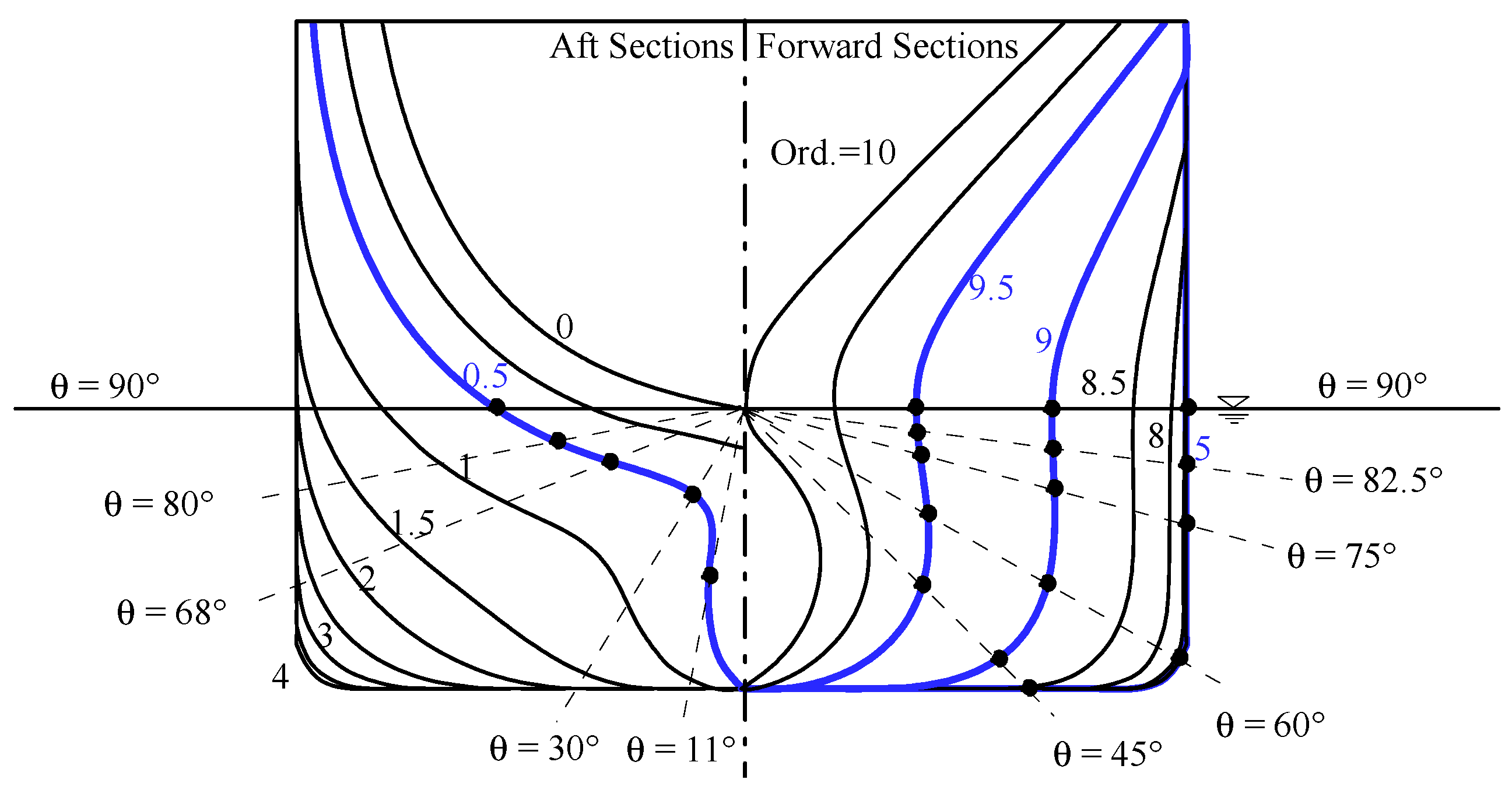
The RIOS bulk carrier, which was the target ship in an innovative experiment [14] to measure the unsteady pressure distribution on the whole ship surface, is considered in this study, and

Table 1. Main particulars of the RIOS (Research Initiative on Oceangoing Ships) bulk carrier.

Particulars	Values
L (m)	2.400
B (m)	0.400
T (m)	0.128
∇ (m3)	0.098
CB	0.800

gives its main particulars. The Froude number, Fn = U/(gL)^1/2, is equal to 0.18. In the experiment [14], a total of 234 pressure sensors were attached on the RIOS bulk carrier. The Fiber Bragg Gratings (FBG) sensor was adapted, which is based on optical-fiber sensing technology. In this study, the wave-induced pressure for some representative positions of the ship surface is compared with the experimental data. The distance between aft perpendicular (AP) and forward perpendicular (FP) is divided into evenly spaced ordinates, which are equal to 0.0 and 10.0 for AP and FP, respectively. In the present comparison, four sections—ordinate (Ord.) = 9.5, 9.0 (near bow), 5.0 (mid-ship), and 0.5 (near stern)—are selected, and the position of pressure measurement in each section is represented as the angle θ from the keel line. That means 0° indicates the keel-line, and 90° indicates the still-water-level, as shown in Figure 1.

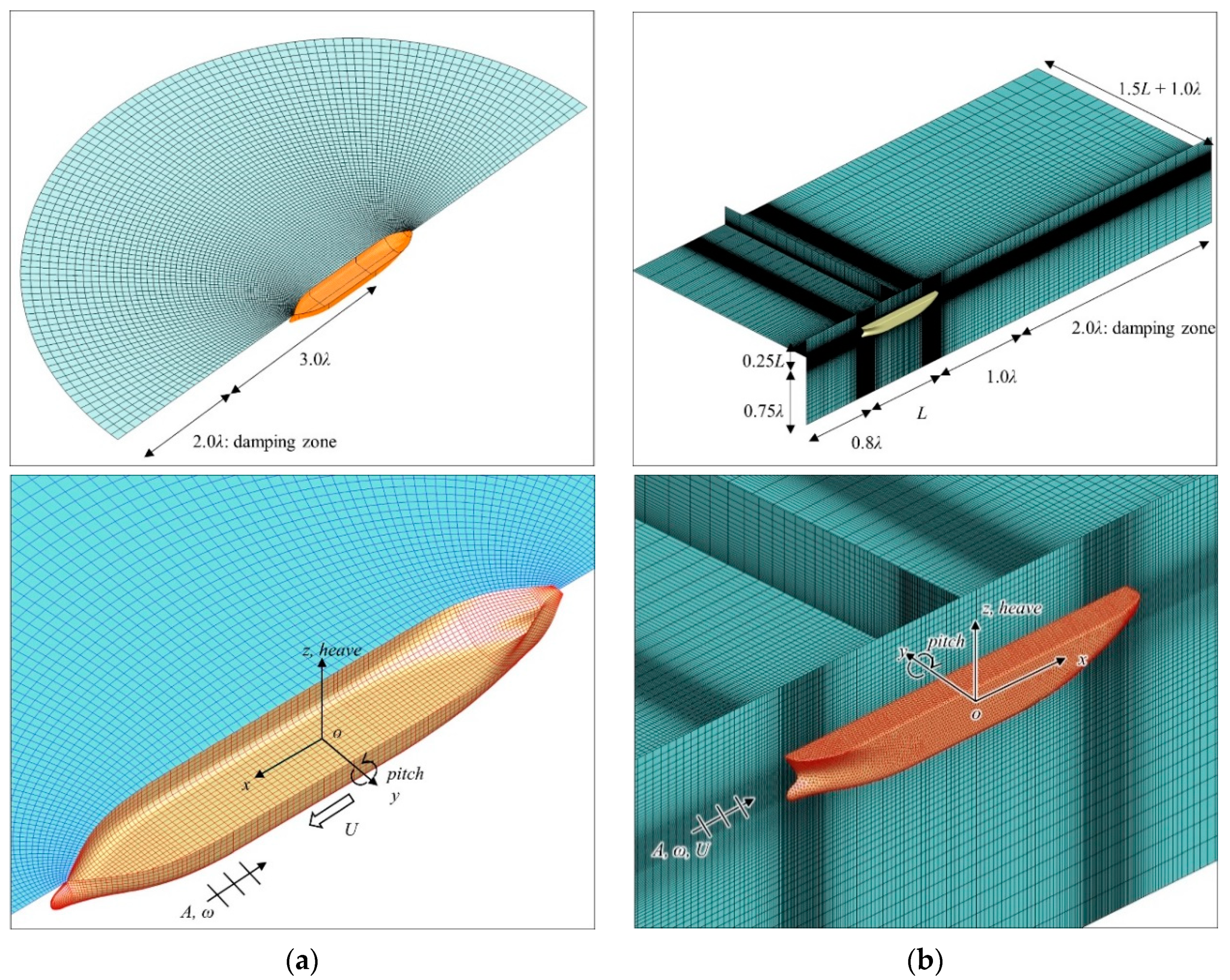
Figure 2 shows domain size and a sample of the triangular surface mesh for the Cartesian-grid method and panel model for the Rankine panel method. Because only head wave cases are considered in this study, half domain is used in both numerical calculations. It should be noted that the present Rankine panel method is based on the linear assumption, and thus the ship below the still-water-level is considered, while the full ship up to ship freeboard is modeled in the Cartesian-grid method.

3.2. Motion Responses and Added Resistance

To check the grid convergence in the Cartesian-grid method, the calculating procedure of grid convergence index (GCI) suggested by Celik et al. [22] was applied for three different grids. The subscripts 1, 2, and 3 indicate the finest grid, medium grid, and coarsest grid, respectively. The average grid spacing $\overline{h}$ for each grid is defined as follows:

$$\overline{h}=\frac{1}{N}{\displaystyle \sum _{\left(i,j,k\right)\in I_C}^N\Delta x_i\Delta y_j\Delta z_k},$$

(12)

$$I_c=\left\{\left(i,j,k\right)|-L/2\le x{c}_i\le L/2,\hspace{0.17em}0\le y{c}_j\le B,\hspace{0.17em}-T\le z{c}_k\le A\right\}.$$

(13)

where N indicates the number of elements in the index set I_c. (i, j, k) is the index pair of the i-th, j-th, and k-th grid point in the x-, y-, and z-direction, respectively. L is the ship length, B is the ship beam, T is the ship draught, A is the amplitude of incident wave, xc_i, yc_j, and zc_k are the center positions, and ∆x_i, ∆y_j, and ∆z_k are the size of the i-th, j-th, and k-th cell, respectively. The grid spacing outside of the range in Equation (13) remains the same to generate the incident wave with the same grid resolution, while the inside grid is systematically refined, which has the ratio of the average grid spacing larger than the square root of two. The total number of grids varied from about two million to five million and the GCI can be obtained using the following procedure:

$$s=1\times \mathrm{sgn}\left({\epsilon }_{32}/{\epsilon }_{21}\right)$$

(14)

$$q=\frac{1}{\ln \left(h_{21}\right)}\left|\ln \left|{\epsilon }_{32}/{\epsilon }_{21}\right|+\ln \left[\left(h_{21}^q-s\right)/\left(h_{32}^q-s\right)\right]\right|$$

(15)

$$GCI=\frac{1.25}{h_{21}^q-1}\left|\frac{V_1-V_2}{V_1}\right|$$

(16)

Here, sgn means sign function,$h_{ij}={\overline{h}}_i/{\overline{h}}_j$,${\epsilon }_{ij}=V_i-V_j$, and V_i indicates a physical variable in the i-th grid.

Table 2. Ratio of average grid spacing and grid convergence index (GCI) of amplitude of vertical motions and added resistance.

λ/L	H/λ	h32	h21	GCI of Heave Amplitude (%)	GCI of Pitch Amplitude (%)	GCI of Added Resistance (%)
0.50	1/80	1.4642	1.5132	-	-	37.7
0.50	1/40	1.4642	1.5132	-	-	26.0
1.25	1/125	1.4967	1.4828	0.0001	0.4632	17.5
1.25	1/80	1.5100	1.4828	0.0120	0.0359	16.5
1.25	1/40	1.4967	1.6438	0.6311	0.0134	12.4

summarizes the ratio of average grid spacing and the resultant GCI values for the magnitudes of heave and pitch motions and added resistance in waves. The heave and pitch motion amplitudes are almost identical, even for different grid spacing, whereas the added resistance is quite sensitive to the grid. The uncertainty of the grid in the added resistance using the Cartesian-grid method is about 10–20% for the resonance case, and about 26% and 38% for the short-wave case. The uncertainty of the grid in the smaller wave amplitude case is larger than that in the large-wave amplitude case. To generate an accurate incident wave in the Cartesian-grid method, the aspect ratio of the grid is important, as well as the number of grids in wave height and wavelength. Thus, it becomes difficult to generate an accurate incident wave for small-wave steepness and short wavelength cases, and the inaccuracy of the incident wave is reflected in the grid uncertainty. However, the maximum difference between the computed added resistance and experimental result is 18% for the resonance case (λ/L = 1.25), with H/λ = 1/125, and the corresponding grid uncertainty is 17%, which is an acceptable range of uncertainty.

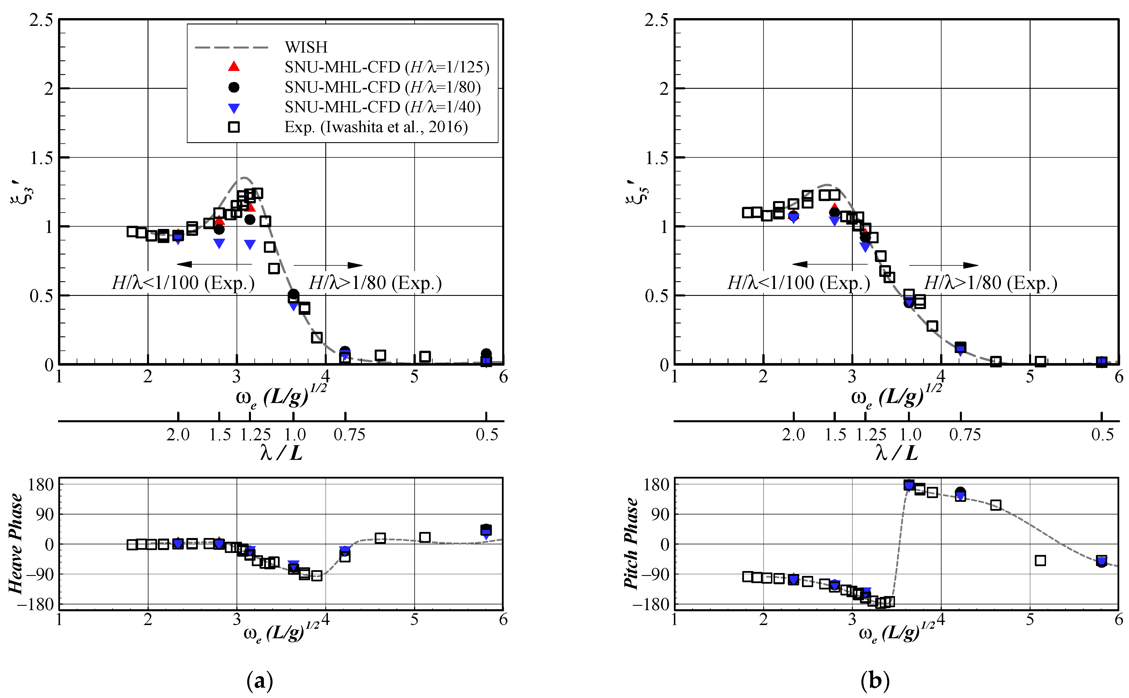
Figure 3 shows the magnitude of the wave-induced heave and pitch motions of the RIOS bulk carrier. The normalized motion magnitudes are defined as follows:

$${\xi }_3^{\prime }=\left|{\xi }_3\right|/A\hspace{0.17em}\hspace{0.17em}\mathrm{and}\hspace{0.17em}\hspace{0.17em}{\xi }_5^{\prime }=\left|{\xi }_5\right|/kA.$$

(17)

Here, k means the wave number of the incident wave and the horizontal axis in the figure represents the normalized encounter frequency ω_e(L/g)^1/2 as well as the normalized wavelength λ/L. The numerical computations using the Cartesian-grid method were conducted with H/λ = 1/80 and 1/40, where H and λ are the wave height and wavelength of the incident wave. In addition, the smaller wave steepness condition (H/λ = 1/125) was simulated for the cases where the wavelength is 1.25 times longer than the ship length. In References [13,14], the wave steepness was varied from H/λ = (1/200 to 1/56). It is difficult using the Cartesian-grid method to generate the incident wave accurately with small-wave steepness in short-wave cases for both experiment and numerical simulation, while in the Rankine panel method, the linearized free-surface and body boundary conditions were applied. The overall magnitude of heave and pitch motions are similar to each other, whereas for the Cartesian-grid method, smaller heave response can be found near the resonance region (λ/L = 1.25). However, if the amplitude of the incident wave decreases, the magnitude of heave motion becomes close to the others. This nonlinearity is known to be responsible for the cross-coupling damping of heave and pitch if the ship has a large flare angle.

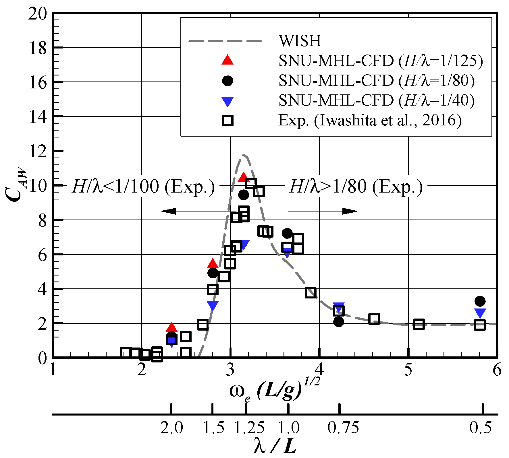
Figure 4 shows the added resistance of the RIOS bulk carrier. The normalized added resistance is defined as follows:

$$C_{AW}=\frac{R_{AW}}{\rho g{A}^2\left(B^2/L\right)}$$

(18)

where R_AW means the dimensional added resistance. Both numerical codes provide similar results to the experiment in the overall wavelength range. Likewise, in the motion responses, the normalized added resistance decreases as the wave steepness increases in the computational results of the Cartesian-grid method. It should be noted that the present Cartesian-grid method solves Euler equations, which means the fluid viscosity is ignored. The ship motion and added resistance in waves are known as inertia-dominant problems and the viscous effects are secondary. But, the viscosity cannot be ignorable depending on the local Keulegan-Carpenter number. This is beyond the scope of the present study and further studies are required using a flow solver of Navier-Stokes equations with a suitable turbulence model.

The difference between experimental data (D) and numerical results (S) is defined as follows:

$$\left(\%D\right)=\frac{\left(D-S\right)}{D}\times 100.$$

(19)

Thus, if the value of numerical results is larger than that of experimental data, the difference becomes negative. The difference values for the amplitude of heave and pitch motions and added resistance are summarized in

Table 3. Difference between experiment and numerical results for amplitude of heave and pitch motion and added resistance.

λ/L	WISH (Wave-Induced loads and SHip Motion)			SNU-MHL-CFD
	ξ3 (%D)	ξ5 (%D)	CAW (%D)	ξ3 (%D)	ξ5 (%D)	CAW (%D)
0.50	-	-	−1.96	-	-	−39.39
1.00	−6.24	14.84	13.62	10.25	7.71	3.96
1.25	−10.25	2.99	−43.55	6.40	4.06	−29.97
1.50	−3.92	−4.81	25.80	5.55	8.35	−24.07
2.00	−0.30	0.05	-	−0.21	7.03	-

. The difference of motion amplitude is smaller than that of added resistance in waves. In general, added resistance in waves is a small quantity to measure from the model tests and thus the uncertainty is also higher than that of motion amplitude.

To investigate the dependency of wave steepness more clearly, Figure 5 plots the magnitude of heave and pitch motions and the added resistance in waves using the Cartesian-grid method for different wave steepness. Figure 5 also represents the corresponding uncertainty of grid spacing as an error bar. As discussed before, the vertical motions and the added resistance decrease as the wave steepness increases, especially for the resonance case (λ/L = 1.25). If the steepness of incident wave increases, the bow wave becomes easily broken, and thus the variation of wetted area is not proportional to the wave amplitude. Moreover, the nonlinearity of bow geometry is one of the reasons that the added resistance in waves is not proportional to the square of the wave amplitude.

3.3. Distribution of Unsteady Pressure

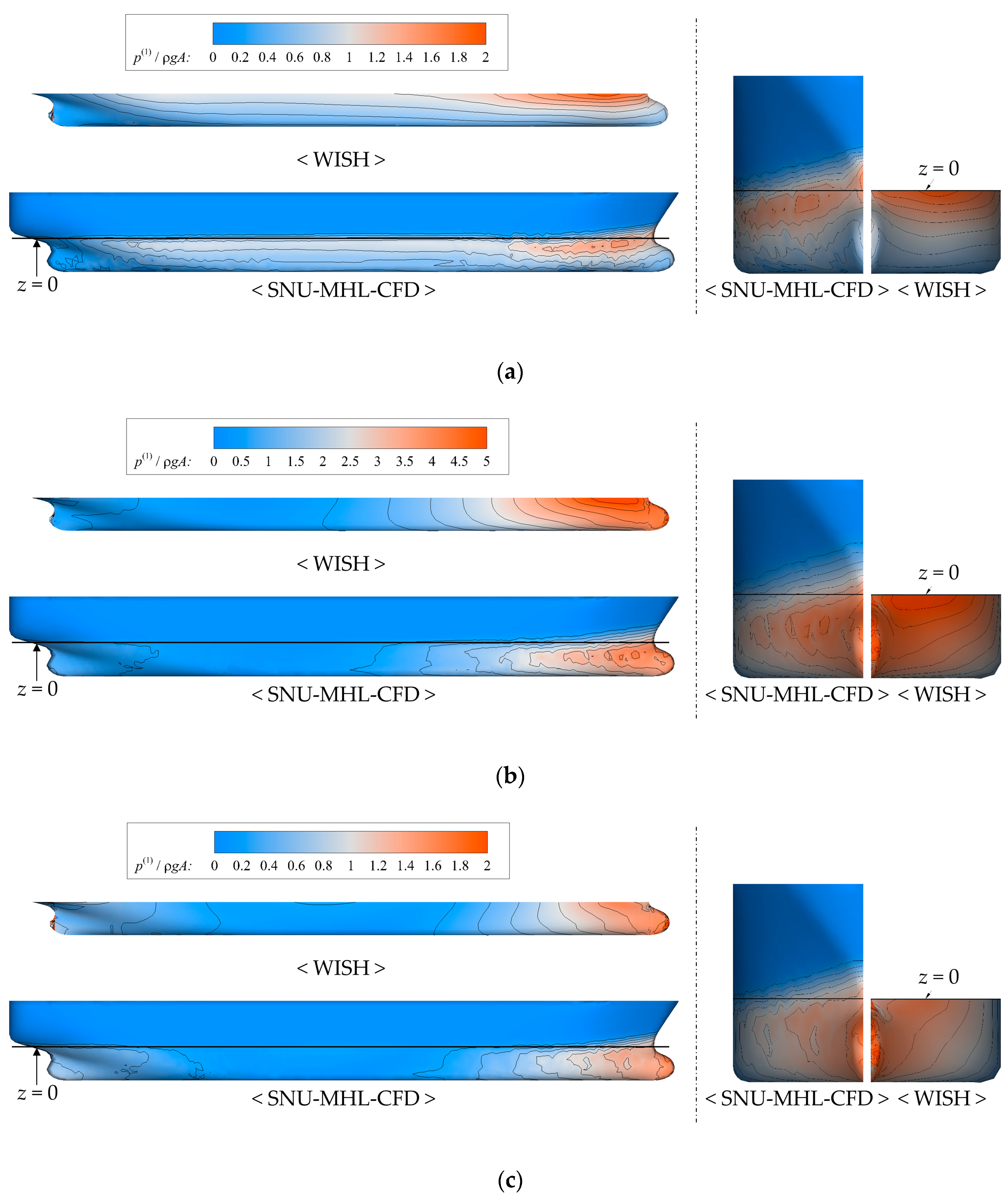
The first harmonic amplitudes of the wave-induced pressure distribution over the whole ship surface for three different wavelengths are compared in Figure 6. The first harmonic amplitude of unsteady pressure is normalized with the maximum value of linear dynamic pressure of the incident wave ρgA. In each figure set, the left column is the side view and the right column is the front view. The upper figure in the left column is the result of the Rankine panel method (WISH), while the lower figure is the result of the Cartesian-grid method (SNU-MHL-CFD). For the short-wave case (λ/L = 0.5), the ship motions can be ignored, and the incident wave is passing through the mid-ship section. Thus, the magnitude of first harmonic pressure is similar to that of the incident wave. On the other hand, the first harmonic amplitude of unsteady pressure is almost zero at the mid-ship for the long-wave condition (λ/L = 2.0) because the ship is surf-riding on the incident wave. The amplitude of the first harmonic from the Rankine panel method near the still-water-level is larger than that from the Cartesian-grid method, especially in the ship bow region, because of the linear assumption. Near the bulbous bow and the ship stern, a slight difference can be observed, whereas the overall patterns below the still-water-level are similar to each other. In the bulbous bow and the ship tern, the aspect ratio of the panel is higher than that in the other parts, and this gives an inaccurate solution.

Figure 7 shows the time history of unsteady pressure for Ord. = 9.5. The left column is the resonance case (λ/L = 1.25), while the right column is the short-wave condition (λ/L = 0.5). The pressure is again normalized with the maximum value of linear dynamic pressure of the incident wave ρgA. The magnitude of normalized pressure is more than three for the resonance case, while it is approximately 1.5 for the short-wave condition. The Rankine panel method provides harmonic time series, while the results of the Cartesian-grid method show the half-sine shape for θ = 90, 82.5, and 75° in the resonance case. Those positions are near the still-water-level, and thus the measuring positions are regularly exposed to the air, because of large ship motion. On the other hand, the exposed time to the air becomes shorter in the short-wave condition, because in this condition, the ship motion can be ignored. The pressure time histories at the other positions show similar magnitude and oscillation period between the two numerical computations.

In the case of stern flow (Ord. = 0.5), the two numerical computations show different magnitudes of wave-induced pressure for the resonance case, even for deeply submerged positions, as shown in Figure 8. In particular, the pressure magnitudes around the crest are different, whereas those around the trough region show similar values to each other. This implies that there are higher harmonic components in the results of the Cartesian-grid method. The magnitude of the unsteady pressure is very small in the stern region for the short-wave condition because of shadowing effects. It should be noted that the time histories of pressure in the Cartesian-grid method show slightly oscillatory behavior. It is known that an immersed boundary method suffers spurious oscillation in pressure fields, especially when a solid body moves, and a grid point is abruptly changed from one phase to another [24].

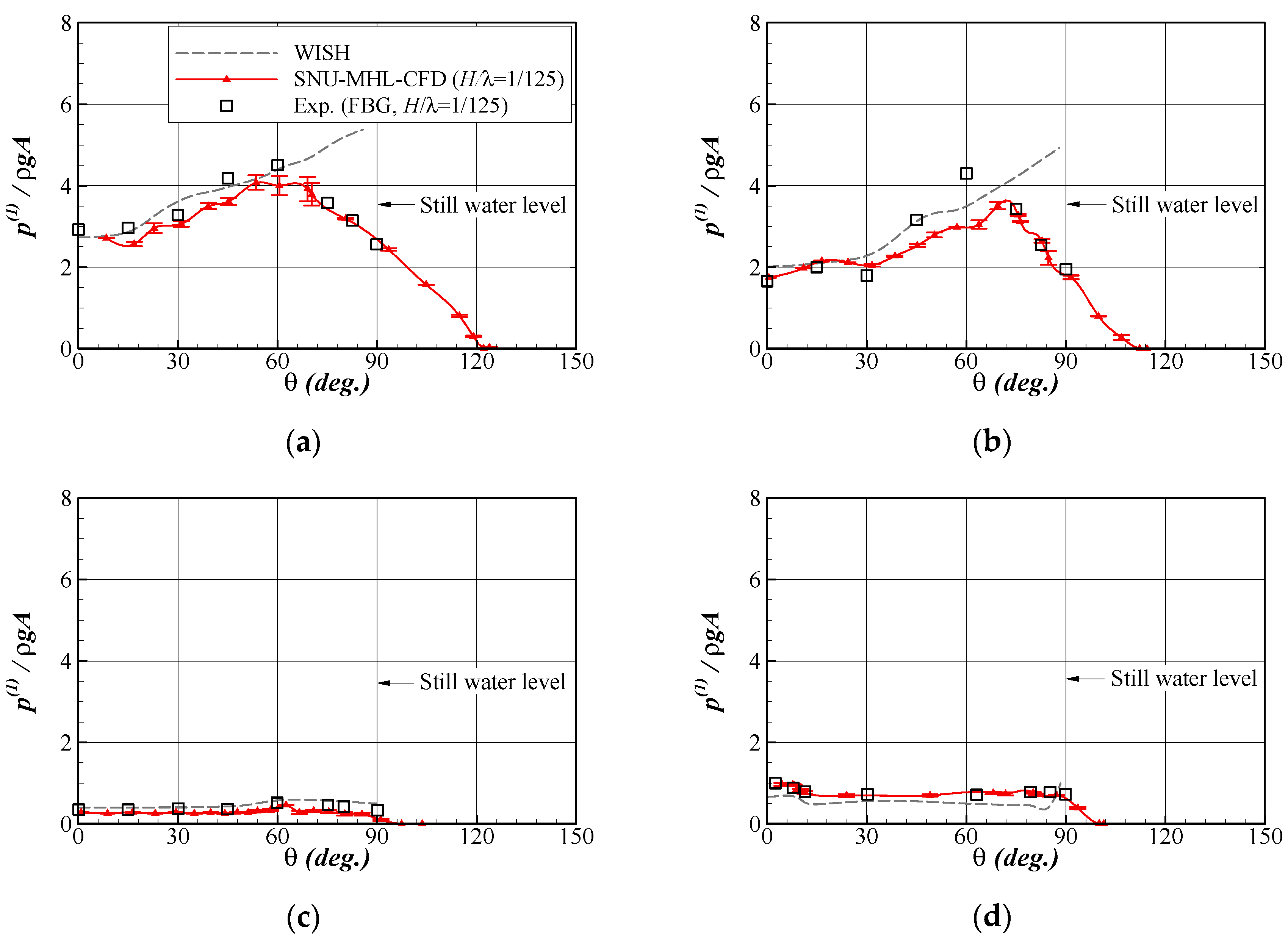
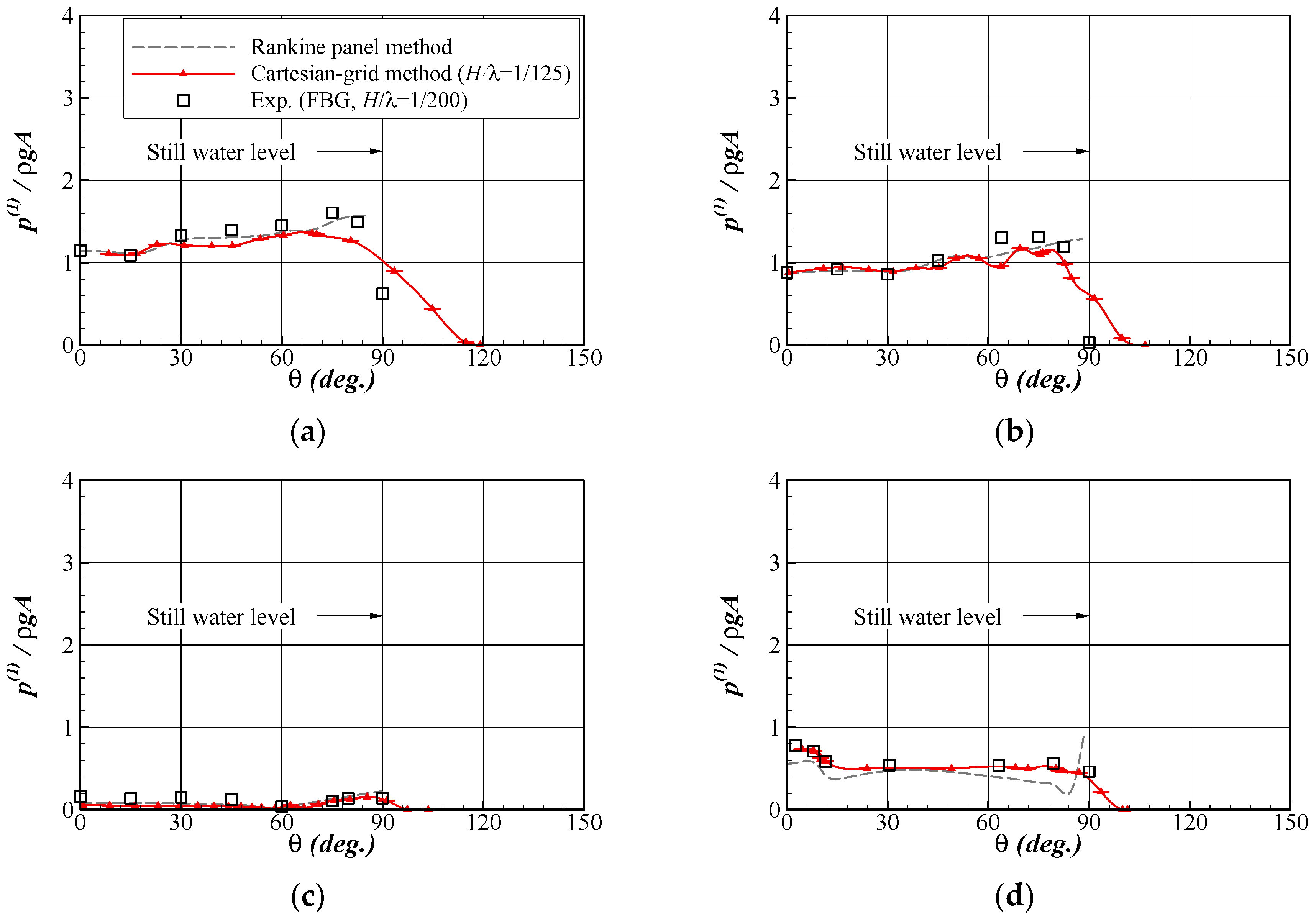
The wave-induced pressure of the Cartesian-grid method and experiment can be decomposed into the Fourier components. Figure 9, Figure 10 and Figure 11 show the magnitude of the first-harmonic component p⁽¹⁾ for different wavelengths. The incident wave steepness is different in the experiment, and it varies from H/λ = (1/200 to 1/56) (λ/L = 2.0 to 0.5), while H/λ = (1/125 and 1/40) cases are simulated using the Cartesian-grid method. The uncertainty of the grid in the Cartesian-grid method is represented as an error bar. The maximum grid uncertainty is 15% near the still-water-level of the bow region in the short-wave condition. Other positions and conditions show less than 5% grid uncertainty.

The magnitude of the first-harmonic component of wave-induced pressure is higher near the ship bow than for the other parts of the ship, and the maximum value is about 1.5 times the maximum value of linear dynamic pressure of the incident wave ρgA for the short-wave (λ/L = 0.5) and long-wave (λ/L = 2.0) cases. In the resonance condition (λ/L = 1.25), the maximum of the first-harmonic pressure is about four times larger than the linear dynamic pressure, because of bow submergence. Near the still-water-level, pressure sensors are regularly exposed to the air, because of the relative motion between ship and water surface, and at those positions, the pressure becomes zero. Thus, the first-harmonic component of pressure near the still-water-level from the Cartesian-grid method and experiment is smaller than that of the Rankine panel method, in which the pressure was calculated for the mean body position. The magnitude of the first-harmonic components of the wave-induced pressure gradually decreases to zero above the still-water-level in the results of the Cartesian-grid method.

A similar tendency can be found in the results at the mid-ship section for the short-wave case (λ/L = 0.5), whereas the value is very small for the resonance condition (λ/L = 1.25) and the long-wave case (λ/L = 2.0). All those results are different from the linear wave theory that the linear dynamic pressure is exponentially decaying in the vertical direction with the factor of kz, where k is the wave number. The discrepancy implies that in these cases, the scattered waves—radiation and/or diffraction waves—are equally important to the incident wave. The first-harmonic component of wave-induced pressure is distributed almost uniformly along the vertical direction in the stern region, and its magnitude is less than or equal to half of the linear dynamic pressure.

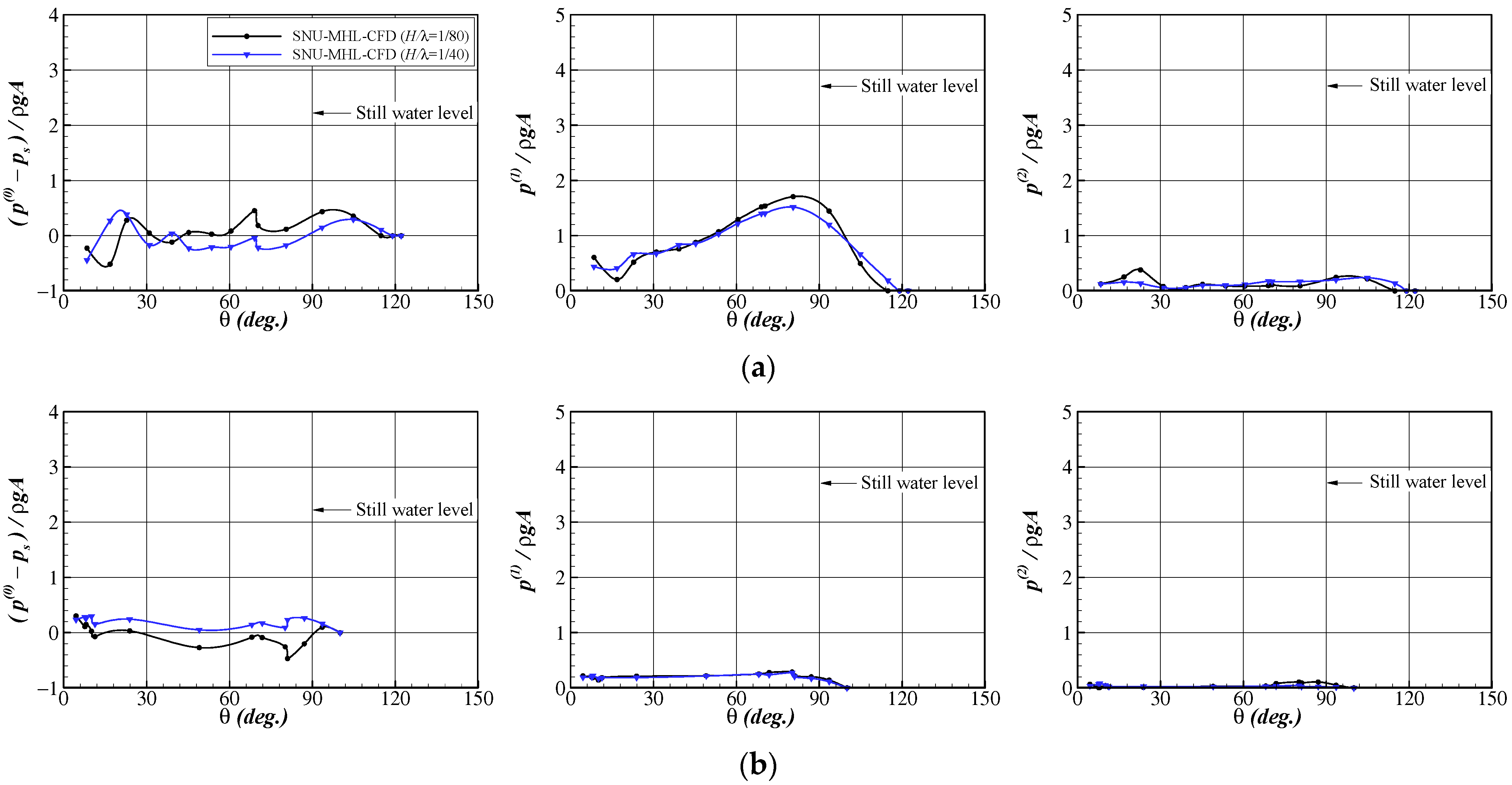
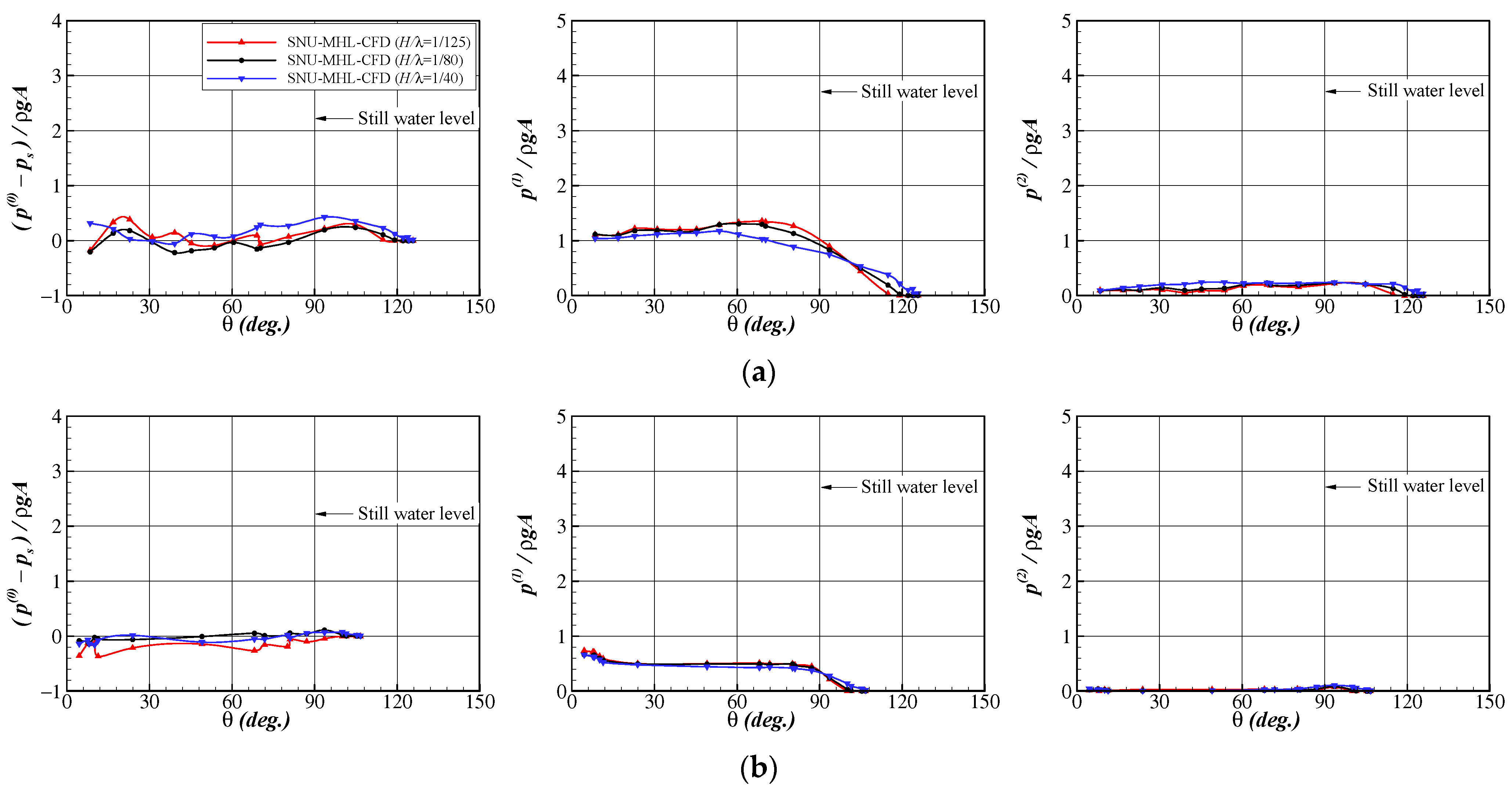
Figure 12, Figure 13 and Figure 14 compare the magnitude of the zeroth-, first-, and second-harmonic components of wave-induced pressure for λ/L = (0.5, 1.25, and 2.0), based on the results of the Cartesian-grid method. The steady pressure p_s in calm water condition is subtracted from the zeroth-harmonic component. This quantity is closely related to the added resistance in waves and has been defined as the time-averaged added pressure. In the case of ship bow (Ord. = 9.5), it is a positive value near the still-water-level because of wave inertia and this effect is exponentially decaying in the vertical direction. There exists negative added pressure due to suction pressure, which is corresponding to the velocity square term in Bernoulli’s equation. However, if the relative ship motion becomes negligible (λ/L = 0.5 and 2.0), the difference of inertia and suction effects is small, which means the added resistance becomes small. In contrast, the added pressure shows relatively large magnitude in the resonance condition, as shown in Figure 13a, and this implies that the added resistance is larger than that in the short-wave or long-wave conditions. It is also clearly observed that the positive added pressure occurs near the still-water-level, while the negative value exists below the still-water-level. Moreover, the vertical distribution range of positive added pressure increases with increasing wave amplitude.

The normalized values of first-harmonic component for the short-wave condition are less sensitive to wave steepness than that for the resonance condition. In other words, the first-harmonic component is proportional to the wave amplitude for the short-wave condition. On the contrary, if the wave amplitude increases, the first-harmonic component decreases for the resonance condition, as shown in Figure 13b. It implies that the first-harmonic component is proportional to the lower order, rather than to the first order of the wave amplitude for this condition. The nonlinear effect of the incoming wave amplitude can be clearly seen in the bow region, whereas this effect is diminished near the stern section. In the stern section, the nonlinear effects of the hull geometry and viscosity are more important than the incoming wave itself. The magnitudes of the second-harmonic components in both the bow and stern regions are very small, compared with that of the first-harmonic component in the bow region. In the long-wave condition, the zeroth- and second-harmonic components are close to zero, and the first-harmonic component is slightly reduced as the incident wave steepness increases. However, the degree of change according to the amplitudes of incident wave is smaller than that in the resonance condition because the relative wave height is different.

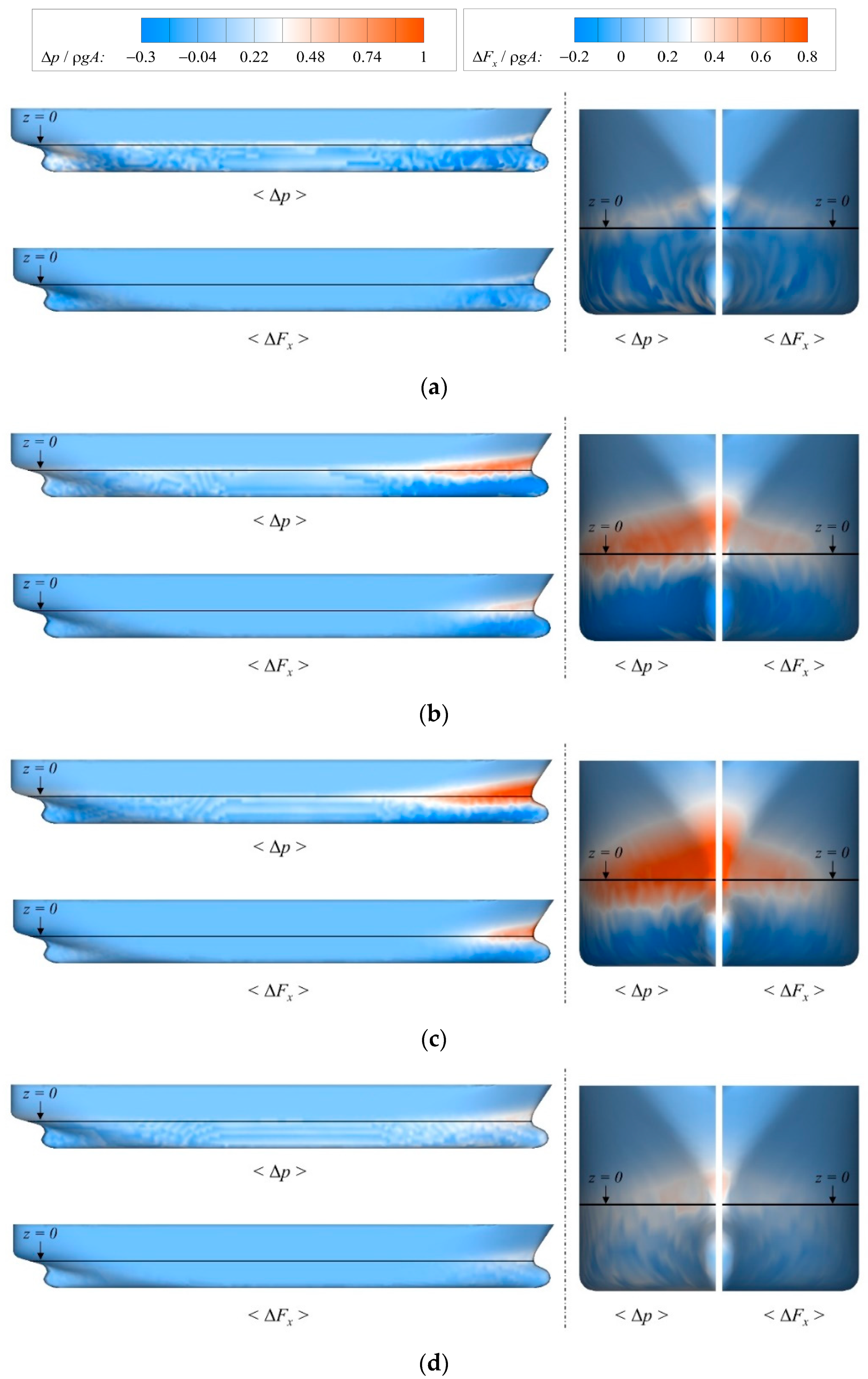
To investigate the characteristic of added resistance in head waves more clearly, Figure 15 plots the time-averaged added pressure and the added local force in the longitudinal direction obtained using the Cartesian-grid method. In the previous study [17], the added pressure Δp_k was defined as follows:

$$\Delta p_k\left(t\right)=p_k\left(t\right)-p_k^0;\hspace{0.17em}\hspace{0.17em}\hspace{0.17em}\hspace{0.17em}\hspace{0.17em}\hspace{0.17em}\hspace{0.17em}\hspace{0.17em}\hspace{0.17em}\hspace{0.17em}\hspace{0.17em}\hspace{0.17em}\hspace{0.17em}\hspace{0.17em}\hspace{0.17em}\hspace{0.17em}\hspace{0.17em}\hspace{0.17em}k=1,2,\cdots ,N_{face}$$

(20)

where p_k(t) is the unsteady pressure at the k-th triangular surface mesh and superscript ‘0′ indicates the steady pressure for the calm-water condition, and N_face is the total number of triangular surface mesh.

The added pressure is a meaningful quantity only for a fixed ship or a ship in short waves, where the ship motion can be neglected. In the present study, the added local force $\Delta {\overrightarrow{F}}_k$ is defined by considering the variation of surface normal vector in time, as follows:

$$\Delta {\overrightarrow{F}}_k\left(t\right)=p_k\left(t\right){\overrightarrow{n}}_k\left(t\right)-p_k^0{\overrightarrow{n}}_k^0;\hspace{0.17em}\hspace{0.17em}\hspace{0.17em}k=1,2,\cdots ,N_{face}$$

(21)

where ${\overrightarrow{n}}_k\left(t\right)$ is the surface normal vector of the k-th triangular surface mesh and superscript ‘0′ indicates the mean value of surface normal vector for the calm-water condition. It should be noted that the surface area is assumed to be unity, because in the present Cartesian-grid method, the change of wetted area is automatically reflected in the pressure value. In this study, only the x-component of added local force is considered, because it is directly related to the added resistance in waves.

As the wavelength increases, the ship motion becomes large, and thus the time-averaged added pressure increases and the considerable added pressure is occurred in the wide range of the bow. If the wavelength is longer than that for the resonance condition (λ/L = 1.25), the ship tends to move up and down following the incoming waves. Thus, the relative wave elevation would decrease and consequently, the added pressure becomes smaller. The added local force shows much more clearly the contribution of the ship bow to the added resistance in waves. Because the variation of the surface normal vector in time is also reflected in the added local force, the contribution from the ship shoulder becomes less significant, whereas the ‘hot spot’ is observed around the ship stem above the design waterline. This result also indicates why the sharp bow, such as the Ax-bow type, reduces the added resistance even in the resonance condition, compared with the conventional bow shape.

4. Conclusions

This study compared the computational and experimental results of heave motion, pitch motion, and added resistance of the RIOS bulk carrier in head waves. Moreover, it investigated the distribution of unsteady, wave-induced pressure on the ship surface. The results show that the overall accuracy of both numerical methods is acceptable, and the following conclusions can be drawn:

• The nonlinearity of pressure distribution was observed mostly from the pressure near the still-water-level of the ship bow, where the measurement position was regularly exposed to the air. Consequently, the pressure time history near the still-water-level showed half-sine shape, and the first-harmonic component was smaller than that from the Rankine panel method, in which the linearized boundary value problem is solved.
• The time-averaged added pressure, which is defined as the difference between the zeroth-harmonic component of the wave-induced pressure and the steady pressure in calm-water condition, tended to show positive value near the still-water-level of the bow, whereas negative value was observed below the still-water-level. This tendency can be clearly seen for the resonance wave condition in this study, and the vertical distribution range of positive added pressure became wider as the amplitude of incident wave increased.
• The normalized first-harmonic component of wave-induced pressure decreased as the wave steepness increased, especially in the ship bow section for the resonance wave condition. This nonlinearity indicates that the variation of wetted surface is not proportional to the amplitude of the incident waves, and it also affects the added resistance due to waves for different wave steepness.
• The added local force, which includes the variation of pressure and surface normal vector in time due to the ship motion, was introduced. The major contribution of the time-averaged added local force that occurs around the ship stem above the design waterline and the distribution of the added local force in the longitudinal direction will provide useful information to understand the added resistance in waves in more detail.

References

- Bunnik, T.; Van Daalen, E.; Kapsenberg, G.; Shin, Y.; Huijsmans, R.; Deng, G.; Delhommeau, G.; Kashiwagi, M.; Beck, B. A comparative study on state-of-the-art prediction tools for seakeeping. In Proceedings of the 28th Symposium on Naval Hydrodynamics, Pasadena, CA, USA, 12–17 September 2010; pp. 1–13. [Google Scholar]
- Kim, Y.; Kim, K.H.; Kim, J.H.; Kim, T.; Seo, M.G.; Kim, Y. Time-domain analysis of nonlinear motion responses and structural loads on ships and offshore structures: Development of WISH programs. Int. J. Nav. Arch. Ocean 2010, 3, 37–52. [Google Scholar] [CrossRef] [Green Version]
- Larsson, L.; Stern, F.; Visonneau, M. Numerical Ship Hydrodynamics—An Assessment of the Gothenburg 2010 Workshop, 1st ed.; Springer: Amsterdam, The Netherlands, 2014. [Google Scholar]
- Faltinsen, O.M.; Minsaas, K.J.; Liapis, N.; Skjørdal, S.O. Prediction of resistance and propulsion of a ship in a seaway. In Proceedings of the 13th Symposium on Naval Hydrodynamics, Tokyo, Japan, 6–10 October 1980; pp. 505–529. [Google Scholar]
- Orihara, H.; Miyata, H. Evaluation of added resistance in regular incident waves by computational fluid dynamics motion simulation using an overlapping grid system. J. Mar. Sci. Technol. 2003, 8, 47–60. [Google Scholar] [CrossRef]
- Kim, K.H.; Kim, Y. Numerical study on added resistance of ships by using a time-domain Rankine panel method. Ocean Eng. 2011, 38, 1357–1367. [Google Scholar] [CrossRef]
- Kashiwagi, M. Hydrodynamic study on added resistance using unsteady wave analysis. J. Ship. Res. 2013, 57, 1–21. [Google Scholar] [CrossRef]
- Seo, M.G.; Park, D.M.; Yang, K.K.; Kim, Y. Comparative study on computation of ship added resistance in waves. Ocean Eng. 2013, 73, 1–15. [Google Scholar] [CrossRef]
- Tanizawa, K.; Taguchi, H.; Saruta, T.; Watanabe, I. Experimental study of wave pressure on VLCC running in short waves. J. Soc. Nav. Archit. Jpn. 1993, 174, 233–242. (In Japanese) [Google Scholar] [CrossRef]
- Kashwagi, M.; Mizokami, S.; Yasukawa, H.; Fukushima, Y. Prediction of wave pressure and loads on actual ships by the enhanced unified theory. In Proceedings of the 23rd Symposium on Naval Hydrodynamics, Val de Reuli, France, 17–22 September 2000. [Google Scholar]
- Chiu, F.-C.; Tiao, W.-C.; Guo, J. Experimental study on the nonlinear pressure acting on a high-speed vessel in regular waves. J Mar. Sci. Technol. 2007, 12, 203–217. [Google Scholar] [CrossRef]
- Tiao, W.-C. Practical approach to investigate the statistics of nonlinear pressure on a high-speed ship by using the Volterra model. Ocean Eng. 2010, 37, 847–857. [Google Scholar] [CrossRef]
- Iwashita, H.; Kashiwagi, M.; Ito, Y.; Seki, Y.; Yoshida, J.; Wakahara, M. Measurement of unsteady pressure distributions of a ship advancing in waves. In Proceedings of the Japan Society of Naval Architects and Ocean Engineers, Fukuoka, Japan, 26–27 May 2016; Volume 22, pp. 235–238. (In Japanese). [Google Scholar]
- Iwashita, H.; Kashiwagi, M. An innovative EFD for studying ship seakeeping. In Proceedings of the 33rd International WorkShop on Water Waves and Floating Bodies, Guidel-Plages, France, 4–7 April 2018. [Google Scholar]
- Orihara, H.; Matsumoto, K.; Yamasaki, K.; Takagishi, K. CFD simulations for development of high-performance hull forms in a seaway. In Proceedings of the 6th Osaka Colloquium on Seakeeping and Stability of Ships, Osaka, Japan, 26–29 March 2008; pp. 58–65. [Google Scholar]
- Sadat-Hosseini, H.; Wu, P.; Carrica, P.M.; Kim, H.; Toda, Y.; Stern, F. CFD verification and validation of added resistance and motions of KVLCC2 with fixed and free surge in short and long head waves. Ocean Eng. 2013, 59, 240–273. [Google Scholar] [CrossRef]
- Yang, K.K.; Kim, Y. Numerical analysis of added resistance on KVLCC2 in short waves with different bow shapes and wave amplitudes. J. Mar. Sci. Tech. 2017, 22, 245–258. [Google Scholar] [CrossRef] [Green Version]
- Hu, C.; Kashiwagi, M. Two-dimensional numerical simulation and experiment on strongly nonlinear wave–body interactions. J. Mar. Sci. Technol. 2009, 14, 200–213. [Google Scholar] [CrossRef]
- Xiao, F.; Honma, Y.; Kono, T. A simple algebraic interface capturing scheme using hyperbolic tangent function. Int. J. Numer. Methods Fluids 2005, 48, 1023–1040. [Google Scholar] [CrossRef]
- Yokoi, K. Efficient implementation of THINC scheme: A simple and practical smoothed VOF algorithm. J. Comput. Phys. 2007, 226, 1985–2002. [Google Scholar] [CrossRef]
- Yang, K.K.; Kim, Y.; Nam, B.W. Cartesian-grid-based computational analysis for added resistance in waves. J. Mar. Sci. Tech. 2015, 20, 155–170. [Google Scholar] [CrossRef]
- Celik, I.B.; Ghia, U.; Roache, P.; Freitas, C. Procedure for estimation and reporting of uncertainty due to discretization in CFD applications. J. Fluids Eng. 2008, 130, 078001–078004. [Google Scholar]
- Joncquez, S.A.G. Second-Order Forces and Moments Acting on Ships in Waves. Ph.D. Thesis, Technical University of Denmark, Lyngby, Denmark, 2009. [Google Scholar]
- Lee, J.; Kim, J.; Choi, H.; Yang, K.S. Sources of spurious force oscillations from an immersed boundary method for moving-body problems. J. Comp. Phys. 2011, 230, 2677–2695. [Google Scholar] [CrossRef]
Figure 1.
Body plan and location of pressure measurement.
Figure 2.
Domain size (upper) and body surface mesh (lower): (a) Rankine panel method, and (b) Cartesian-grid method.
Figure 3.
Motion amplitude (upper) and phase angle (lower) of the RIOS bulk carrier: (a) heave, (b) pitch.
Figure 4.
Added resistance of the RIOS bulk carrier in waves.
Figure 5.
Dependency of wave steepness and grid uncertainty in the Cartesian-grid method: (a) Magnitude of heave motion (λ/L = 1.25), (b) magnitude of pitch motion (λ/L = 1.25), (c) added resistance in waves (λ/L = 1.25), and (d) added resistance in waves (λ/L = 0.5).
Figure 6.
Distribution of the first-harmonic component of wave-induced pressure, side view (left) and front view (right): (a) λ/L = 0.5, (b) λ/L = 1.25, (c) λ/L = 2.0.
Figure 7.
Time histories of wave-induced pressure distribution on the RIOS bulk carrier, ordinate (Ord.) = 9.5, λ/L = 1.25 (left) and λ/L = 0.5 (right): (a) θ = 90°, (b) θ = 82.5°, (c) θ = 75°, (d) θ = 60°, (e) θ = 45°.
Figure 8.
Time histories of wave-induced pressure distribution on the RIOS bulk carrier, ordinate (Ord.) = 0.5, λ/L = 1.25 (left) and λ/L = 0.5 (right): (a) θ = 90°, (b) θ = 80°, (c) θ = 68°, (d) θ = 30°, (e) θ = 11°.
Figure 9.
Magnitude of the first-harmonic pressure component for the RIOS bulk carrier in waves, λ/L = 0.5.: (a) Ord. = 9.5 (bow region), (b) Ord. = 9.0 (bow region), (c) Ord. = 5.0 (mid-ship), (d) Ord. = 0.5 (stern region).
Figure 10.
Magnitude of the first-harmonic pressure component for the RIOS bulk carrier in waves, λ/L = 1.25.: (a) Ord. = 9.5 (bow region), (b) Ord. = 9.0 (bow region), (c) Ord. = 5.0 (mid-ship), (d) Ord. = 0.5 (stern region).
Figure 11.
Magnitude of the first-harmonic pressure component for the RIOS bulk carrier in waves, λ/L = 2.0.: (a) Ord. = 9.5 (bow region), (b) Ord. = 9.0 (bow region), (c) Ord. = 5.0 (mid-ship), (d) Ord. = 0.5 (stern region).
Figure 12.
Magnitude of the harmonic components of wave-induced pressure for the RIOS bulk carrier in waves, λ/L = 0.5, 0th harmonic (left), 1st harmonic (middle), and 2nd harmonic (right): (a) Ord. = 9.5, (b) Ord. = 0.5.
Figure 13.
Magnitude of the harmonic components of wave-induced pressure for the RIOS bulk carrier in waves, λ/L = 1.25, 0th harmonic (left), 1st harmonic (middle), and 2nd harmonic (right): (a) Ord. = 9.5, (b) Ord. = 0.5.
Figure 14.
Magnitude of the harmonic components of wave-induced pressure for the RIOS bulk carrier in waves, λ/L = 2.0, 0th harmonic (left), 1st harmonic (middle), and 2nd harmonic (right): (a) Ord. = 9.5, (b) Ord. = 0.5.
Figure 15.
Distribution of the time-averaged added pressure and added local force in the x-direction for the RIOS bulk carrier, H/λ = 1/40: side view (left) and front view (right): (a) λ/L = 0.5, (b) λ/L = 1.0, (c) λ/L = 1.25, (d) λ/L = 2.0.