Article

Evolutionary Algorithm to Support Field Architecture Scenario Screening Automation and Optimization Using Decentralized Subsea Processing Modules

by
Mariana J. C. Díaz Arias
1,*,
Allyne M. dos Santos
2 and
Edmary Altamiranda
3,*
1
Department of Geoscience and Petroleum, Norwegian University of Science and Technology, 7031 Trondheim, Norway
2
Department of Chemical Engineering, Norwegian University of Science and Technology, 7491 Trondheim, Norway
3
Technology Department, Operations & Asset Development, Aker BP ASA, 4020 Stavanger, Norway
*
Authors to whom correspondence should be addressed.
Submission received: 16 December 2020 / Revised: 11 January 2021 / Accepted: 15 January 2021 / Published: 19 January 2021
(This article belongs to the Section Advanced Digital and Other Processes)

Abstract

:
Manual generation of test cases and scenario screening processes, during field architecture concept development, may produce a limited number of solutions that do not necessarily lead to an optimal concept selection. For more complex subsea field architectures, which might include processing modules for enhancing pressure and thermal management for the production network, the number of configuration cases and scenarios to evaluate can be extremely large and time and resource-consuming to handle through conventional manual design processes. This paper explores the use of evolutionary algorithms (EA) to automate case generation, scenario screening, and optimization of decentralized subsea processing modules during field development. An evaluation of various genetic operators and evolution strategies was performed to compare their performance and suitability to the application. Based on the evaluation results, an EA using structural uniform crossover and a gradient plus boundary mutation as the main variation operators was developed. The methodology combines EA and an integrated modeling approach to automate and optimize the concept selection and field architecture design when considering decentralized subsea processing modules.

1. Introduction

Typical field architecture concepts, where wells from different reservoir and production regions are connected to the same production network, may offer a suboptimal solution when it comes to pressure and thermal management of the production fluids. Thus, for fields with large heterogeneity among the wells, the common cluster solution may create a strong interdependence between the production rates and wellhead pressures. For such cases, the full performance of the field is compromised by any change in the operating conditions of a given region or wells within the production network. A different approach is being proposed by [1,2], where a well or a region with a large heterogeneous performance is decoupled from the main network by installing decentralized subsea processing modules in the field architecture. This approach, called the Subsea Gate Box (SGB) [3], is addressed to increase production management flexibility by expanding the possible production strategies, considering both production constraints and reservoir dynamics, and increasing the energy efficiency to improve resource utilization.
The process modules within the gate box (or processing station) depend on the field constraints and flowing characteristics. On the other hand, reservoir strategies may require reducing the production rates of wells with given characteristics (sand production, erosion problems, water cut, etc.) or increasing production from other regions. Therefore, the number of constraints and variables to consider during the design phase can escalate considerably, making it difficult to select the best fit-for-purpose solution.
There exists a variety of commercial software to create what is called an integrated production model (IPM) of the asset. These tools are useful to integrate and evaluate the performance of different stages of the production systems, from the reservoir to the topside facility, including the wells and network performance. The integrated models facilitate the evaluation of the interactions along the system and the effects of given variables on given objectives. Works like [4,5,6,7,8,9,10,11,12] demonstrated the value of conducting integrated modeling, from the conceptual and front-end design up to the lifetime field operations, especially for conducting production optimization studies and uncertainty analyses.
The work in [4] presented an early phase conceptual design method using integrated modeling for a full production system from reservoir to the receiving facility, including a subsea gas compression station. The authors concluded that, following this integrated modeling approach, it is possible to ensure robust and optimized field design and operability through the production period. Nevertheless, they emphasized the necessity of simulating all operational scenarios. Likewise, [5] presented a study for a concept screening of the greenfield development, where they employ integrated simulations to enable a holistic investigation of the possible solutions. For their study cases, they nominated four options: natural flow, boosting with multiphase pump, separation with single phase boosting, and separation with boosting and water injection. They concluded that the strong interdependence among the different components across the hydrocarbon production system, especially when including subsea processing, might lead to unrealistic system behavior if one or more components are isolated from the design investigation. The authors of [6] presented a very interesting tool that combined the integrated modeling approach of the full production system with a direct connection between the hardware definition (equipment/technology selection) and cost estimation within the field layout and the production analysis. In this way, the tool allows creating multiple scenarios that can be ranked and evaluated in term of economics and technical aspects for a final concept selection.
The above referred works present a robust and practical methodology for evaluating different scenarios at an early stage of the concept selection process. Nevertheless, they do not offer a clear solution on how to generate all possible scenarios and how to reduce the entire domain of possibilities, which may be very large, to a handful of cases that should be considered further within the integrated models. Such a screening process could be part of a field design optimization, which should consider field architecture key elements (placement of wellheads and manifolds, type and location of production facilities, well scheduling, subsea processing elements, line routing, etc.). Works like [7,13,14,15] have presented different proposals for optimizing field designs. Most of them have used conventional optimization methods that require explicit analytic models to be available. However, in practice, relevant domain engineering software and simulation tools are used to support the field development process. Therefore, it is desirable to utilize data and information generated by different engineering sources during the optimization process. Hence, the availability of explicit analytic models from commercial engineering tools may not be possible.
Evolutionary algorithms (EA) have been successfully used to provide metaheuristic optimization solutions to complex problems, where model-based optimization methods are not suitable, due to the nonavailability of explicit analytic models. EA have also been used for large-scale optimization problems where traditional mathematical methods may have challenges. The purpose of EA is to guide the search, evolving a set of solutions to satisfy the optimization problem objectives. There have been several contributions in the literature addressing the automatic generation of test cases and optimization using EA within software development, such as [16,17,18,19,20,21,22,23,24]. In [21], an EA for linear systems identification was proposed for the screening of different model structures, as well as the models’ parameter estimations. A multi-objective EA for the selection of equipment modules of discrete numbers and sizes, for a flexible production plant, was documented in [22]. An application of EA to optimize an industrial gas turbine blade cooling passage design configuration was presented in [23]. In [24], an EA to optimize a subsea design from a flow assurance point of view was proposed, where the key challenge was the temperature maintenance across the network. Similar approaches were proposed in [25,26,27,28,29], using artificial intelligence-based algorithms to optimize the field design. Nevertheless, the mentioned works optimized only the system portion of interest and did not consider integrated modeling for evaluating the effects of the optimized parameters in the entire system.
Based on the above documented challenges and inspired by the solutions that EA has provided to similar problems, a methodology for automated case generation, scenario screening, and the optimization of subsea processing systems to support field architecture concept development is proposed. The methodology combines evolutionary algorithms (EA) and the integrated modeling approach for screening and selecting the cases. The strategy offers the possibility of different levels of optimization: a level dedicated to optimizing the field architecture (in terms of process module configurations and locations) and a level to optimize the performance of the combined reservoir–network model. The first level is carried out by applying EA, while the latter is achieved by a nonlinear optimizer and a sequential linear programming given by the integrated model.
The development of the EA was performed based on an evaluation over various genetic operators and evolution strategies to compare their performance and suitability to the application. The proposed EA uses structural uniform crossover and gradient plus boundary mutation as the main variation operators. Although the main optimization problem is based on decentralized subsea processing modules, the methodology here presented could also be applied to a central processing station design, as well as adapted to include other field architecture variables. The methodology addressed three main aspects: development of the case generation algorithm, definition of the fitness function (using production integrated modeling), and the design and development of the evolutionary algorithm applied to this optimization problem.
The EA algorithm developed at this stage does not guarantee a global optimal solution, but it supports a methodology to automate and optimize decentralized subsea processing module configurations and locations within a field, avoiding manual case generation and screening processes. The solution obtained for the SGB configuration and location is assumed fixed during the field life at this stage. Future works will focus on the further development of this algorithm to improve the global search and optimization capabilities, include an uncertainty analysis, and consider SGB configuration changes that may be needed throughout the field life.

2. Methods

2.1. Problem Statement: The Subsea Gate Box Concept

The subsea gate box (SGB) is a multifunctional assembly that enables decoupling the well performance from the flow constraints imposed by the common network. The assembly aims to prepare the wells stream to be introduced into the production system by incorporating different process modules, such as separation, boosting, chemical injection, metering, or any other process that might contribute to improving the performance of the production stream. Those process units are conceived as the primary processing stages, since the ultimate objective of the SGB is to enhance the available reservoir energy while avoiding reducing production due to the limitations of the network [2].
The SGB concept targets different field architecture arrangements, and it is not limited to a single wells stream but might also handle regions or production wells with similar characteristics. The SGB modular principle opens up the opportunity to adapt the processing train to specific operating conditions of the treated stream over the lifetime of the field. Figure 1 presents a schematic representation of the SGB, where it is considered an example that assumes a field development with different formations and reservoirs.
The subsea field architecture for such a case depends on four main variables:
  • location of the SGB within the field
  • number of simultaneous SGB within the field
  • number of process modules in a SGB
  • process train sequence in a SGB
Where (1) and (2) are the key parameters for enabling flexibility in the system to allow creating different strategies for production regions with very different performances. They are a function of the process modules available at each SGB. On the other hand, (3) and (4) constitute the internal configuration of a SGB. They are a function of the operating stream: multiphase, gas, oil, or water line. For this work, the internal configuration of the SGB can be a combination of the process shown in Figure 2. The selection of the process depends on the location (input stream) and the global and local constraints within the network.
The combination of all possible options of these four variables creates a considerably large domain of alternatives. Manual selection of the most suitable solutions threatens the possibility for innovation, and it might limit the real purpose of the subsea gate box: increasing the production management flexibility. Therefore, the SGB design requires a systematic and automated screening process that allows exploring the entire domain, ranking the alternatives, and supporting the identification of the best suitable solutions in a consistent manner.

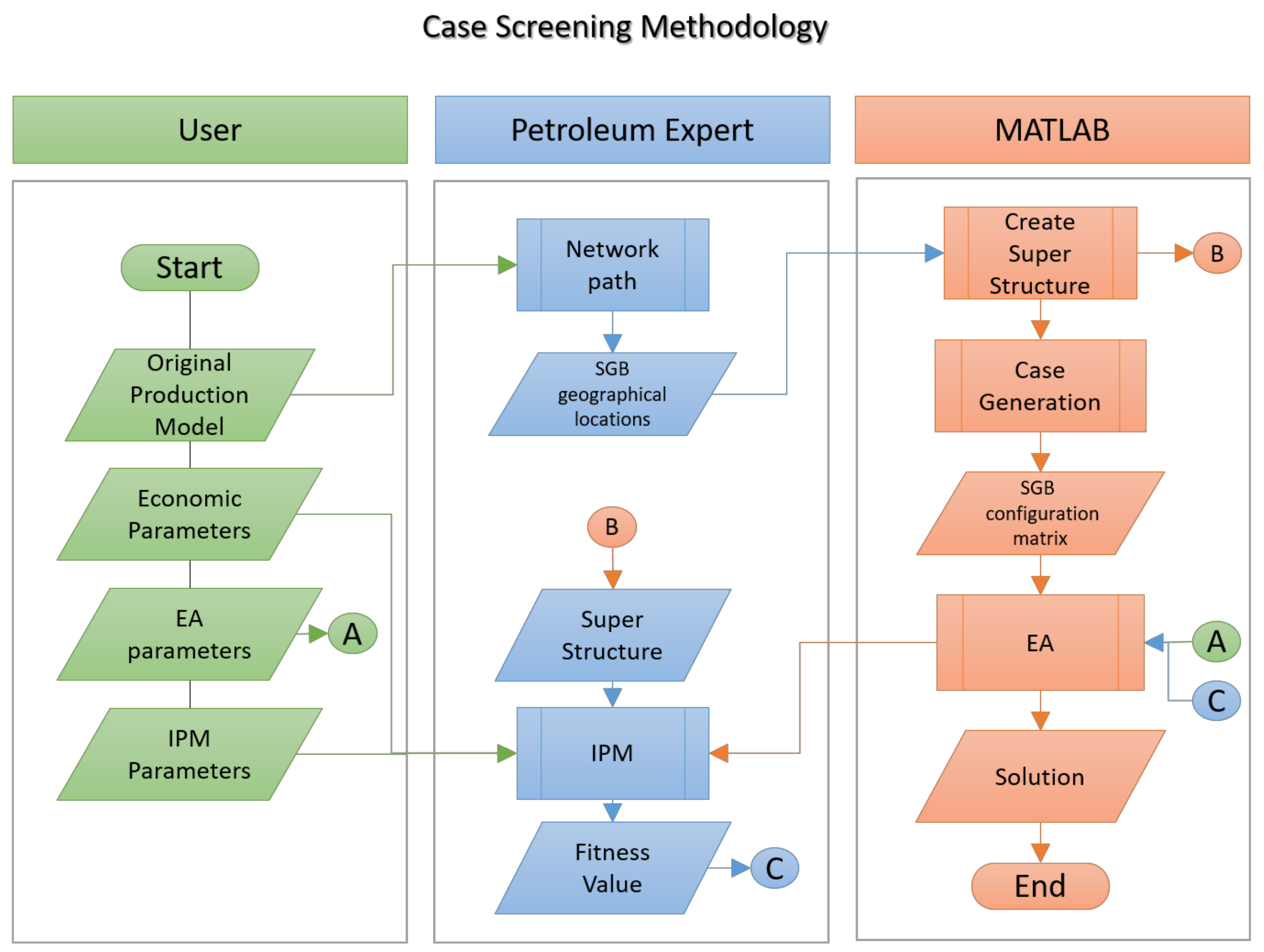
2.2. Case Screening Methodology

The methodology consists of integrating well-known production models used within project development and operation activities with an optimization algorithm. The industry normally relies on commercial software for production models that include multidisciplinary packages covering from the reservoir, wells, flow network, and up to the process facilities. Those packages are normally built as a black box-type software, with limited possibility for accessing the explicit analytic model. This makes difficult the application of traditional optimization methods. In order to keep the possibility of using the production models provided by the commercial software for the screening and optimization process, it is then necessary to use a metaheuristic approach for the optimization of the problem.
The optimization problem of the SGB is based on finding the best combination of the four variables mentioned in Section 2.1 that enables the maximum production rate with the minimum investment. Therefore, the methodology is addressed to find the best geographical locations and configurations of SGBs within a given production system. Thus, the field architecture and the production model for a given field development should be provided by the user.
In this work, the production system is fixed. Thus, the field layout, wells and manifold placements, and production constraints remain constant throughout the field life. The only modifications to the field architecture are the placement of the SGBs and their connection elements, such as additional umbilical lines, pipelines, risers, and connectors.
At this initial stage of the study, some simplifications are included:
  • The diameter of the lines remains from the original design, even when the flow rates of the original lines change due to the SGB operation. Likewise, additional lines downstream of separation processes are taken as a copy of the original.
  • SGBs are installed at the beginning of the project, and their location, configuration, and the settings of the process modules do not change over time.
  • All the optimization settings within the production model are disabled.
  • The production model is set to produce to maximum potential.
  • The process equipment within the SGB are not fully modeled. The process performances are defined as “nodes” in the network that increase the pressure, split phases, or change the temperature. Therefore, the typical values of efficiency from the literature are used for calculating the power demand and estimating the umbilical requirements.
  • The economic model is simplified, as documented in Section 2.5.1.
The methodology requires an integrated production modeling software (IPM), Excel, MATLAB, and a utility software that allows other programs (such as Excel and MATLAB) access to public functions in the IPM.
An IPM is a common approach in the oil and gas industry to evaluate the performance of the production system and the interconnection among its subsystems. The IPM is a digital representation of the hydrodynamics and state conditions of the production fluids at different levels of the system. The model includes system interactions and defines the boundary conditions for each individual system. The reservoir, the distribution network, the processing facilities, and even the economic framework could be defined as a subsystem within an IPM approach.
For this work, the IPM tool from Petroleum Expert, together with their OpenServer utility tool, was used to test the methodology. Figure 3 summarizes the proposed methodology and shows the interconnections among the different tools and their expected inputs and outputs. The following sections explain the parts and functions of the method.

2.3. Data Collection

The first step of the methodology is the data collection and definition of the relevant parameters by the user. The method needs as an input the original production model of the field developed in the IPM tool; the economic parameters (such as oil and gas prices, discount rates, equipment costs, material costs, etc.); the additional model parameters (such as operating constraints, equipment performance limits, production schedule, etc.); and the setting parameters for the EA.

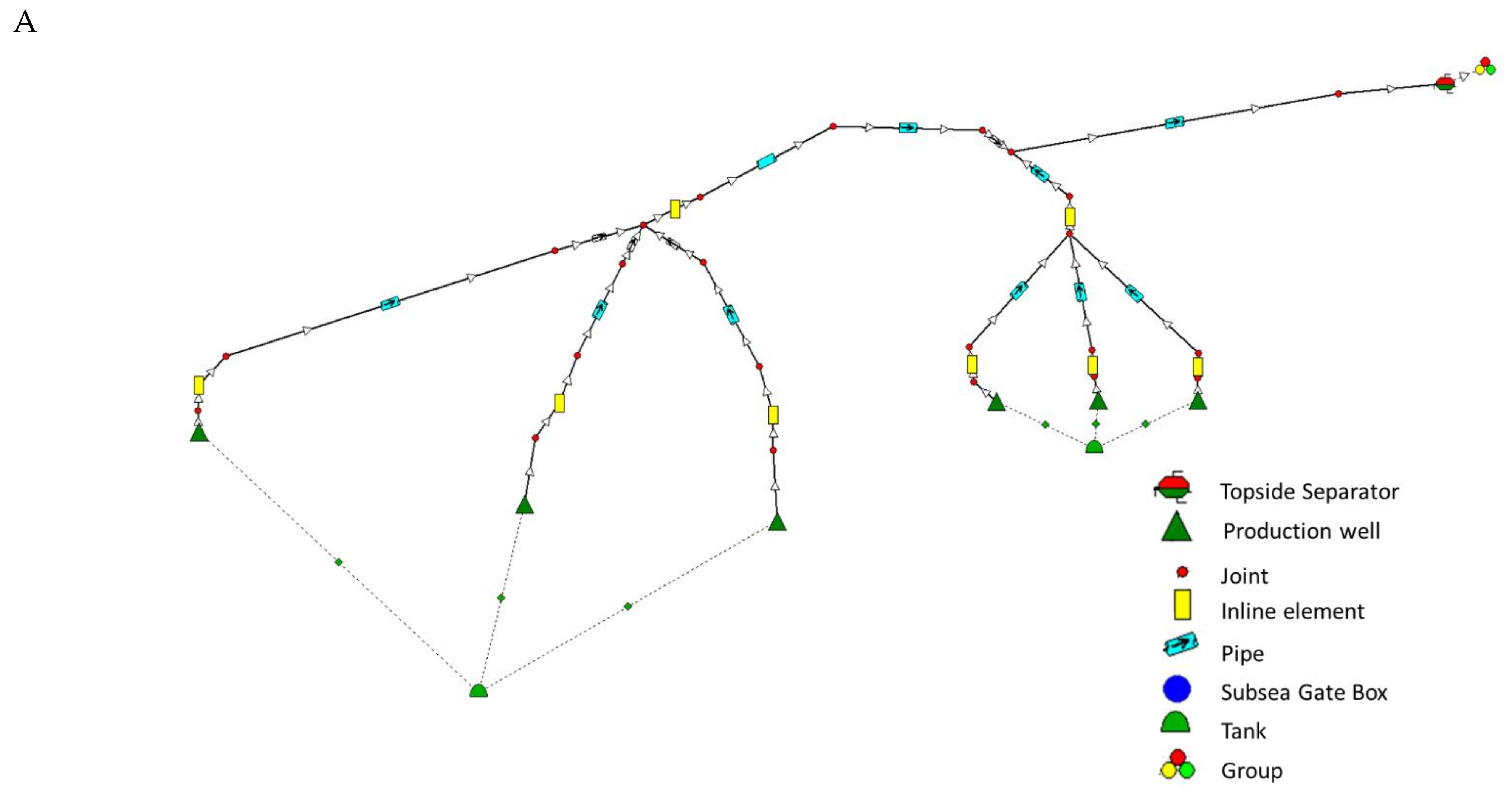
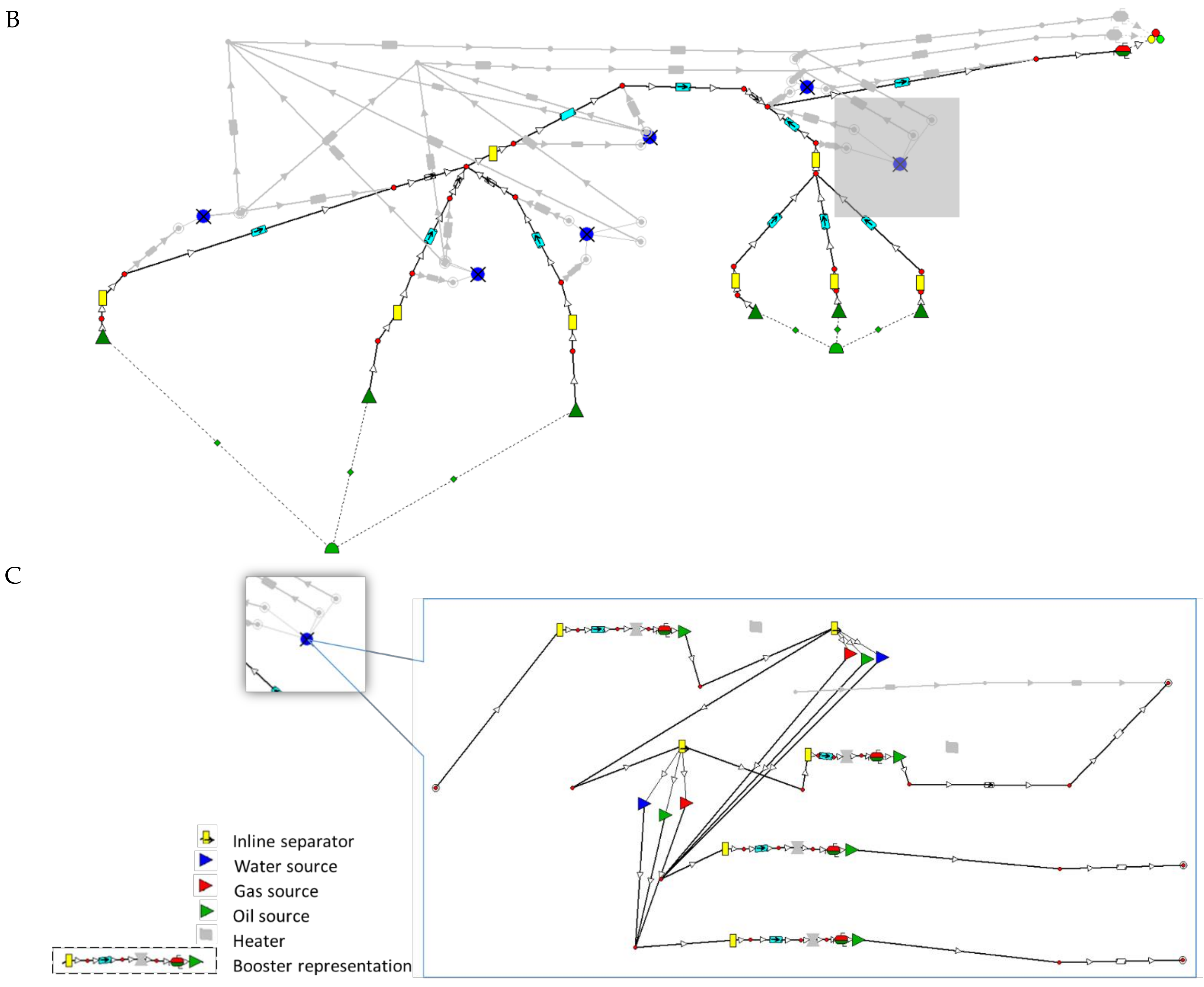
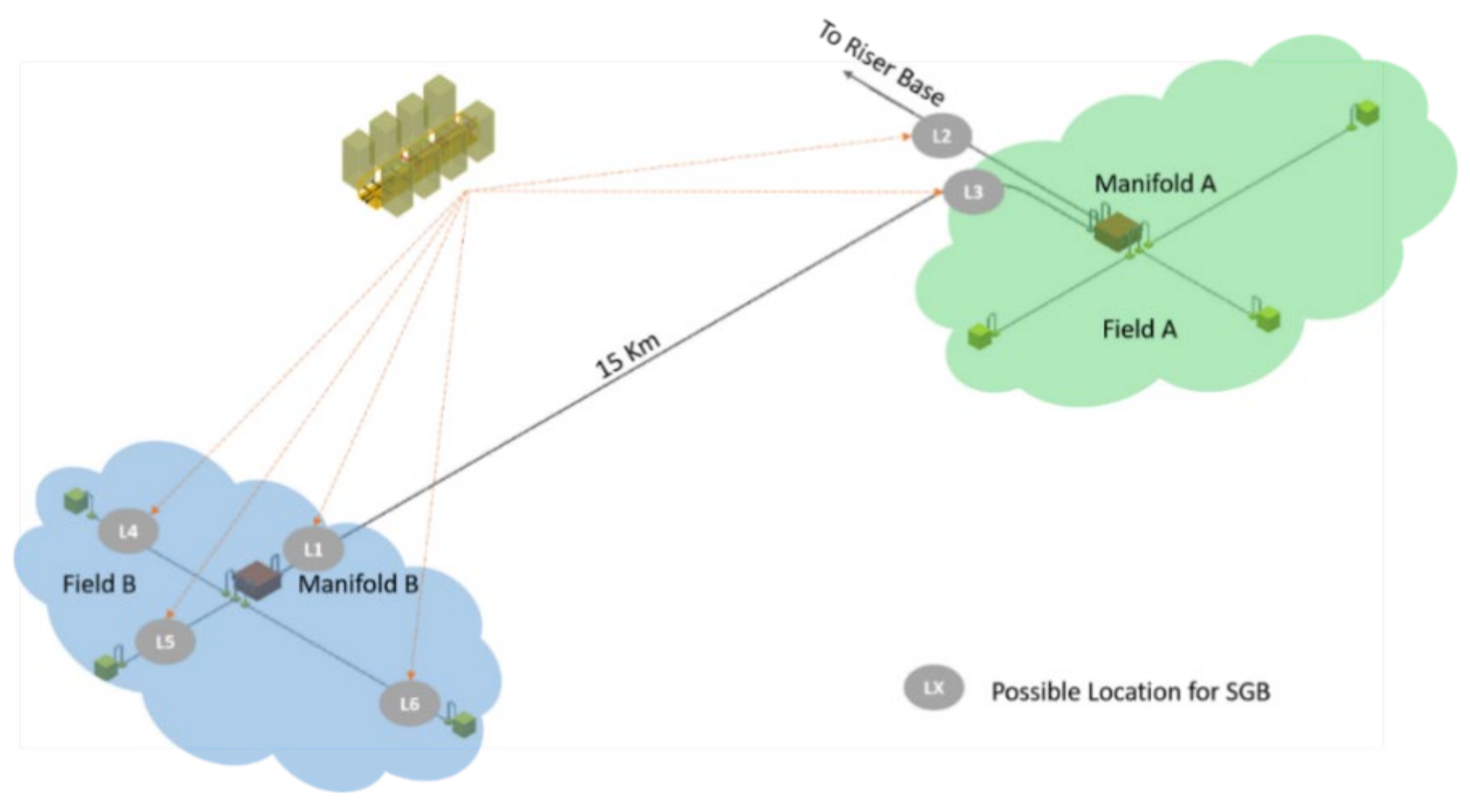
2.4. Identifying Locations and Creating a Superstructure

The second step is the mapping of the original model to identify all possible locations for installing a subsea gate box. Thus, the “Network Path” routine reads the original file and identifies the network path from each of the production wells to the receiving separator. It saves the identification number of the different elements (pipes, joints, wells, and equipment) and lists all production wells and commingling points in the network that can be a potential location for an SGB. The routine is implemented using Visual Workflow of the Petroleum Expert IPM package, and the output of this function is an array with the ID of the different locations within the field to be considered for an SGB.
Subsequently, a copy of the original file is transformed in a superstructure that represents all possible scenarios. A superstructure representation is a highly redundant process diagram that includes all potentially useful processing units and all relevant interconnections. This technique is used in the optimization of process synthesis problems [30,31,32,33,34]. The optimization model is formulated based on this superstructure and includes not only the optimization variables of the synthesis problem but, also, the discrete variables used to select a subset of process units within the superstructure [30].
The superstructure is created by including in the network all possible SGB identified in the “Network Path” function and including all the processes considered in Figure 2 for each SGB. The SGB is represented in the network model as “flowsheet” elements and contains a representation of all the process units and their respective connections, as is shown in Figure 4.
Each geographical location of the SGB in the field network is identified with a correlative number. Likewise, all relevant elements inside the SGB are identified with an integer number and a level name related to the SGB location number. The EA uses this identification system to generate the control variables to activate a given SGB with a given configuration. The superstructure in Figure 4 is then modified by activating or deactivating the SGB elements and by connecting different fluid routes inside the SGB according to the configuration defined for each evaluation case (or individual), as shown in Figure 5.

2.5. The Integrated Model (IPM)

The scope of the present research focuses on subsea processing systems; therefore, the IPM is defined from the reservoir up to the receiving separator topside. The receiving separator is the starting point for the topside process facilities, and it defines the connection point between the subsea production system and the process systems of the production fluids. Thus, the pressure at the receiving separator represents a boundary condition for the subsea production system. Likewise, the flow rate and pressure from the reservoir define another boundary condition of the subsea network.
In this work, the IPM is divided into two sections: the production model and the fitness function. The production model includes the reservoir, the wells, and the subsea network up to the receiving separator. The model uses black oil for the production fluids and a material balance approach to represent the reservoir behavior. The fitness function, on the other hand, is defined by a simplified economic model that includes Capital Expenditure (CAPEX), Operational Expenditures (OPEX), and income calculation generated by the implementation of the subsea gate box. Figure 6 shows a diagram of the model sections and the relations among them. The model is run by RESOLVE, a software that links all applications of the production model with the fitness function. The latest is programmed in a datasheet in Excel that contains the simplified economic model.

2.5.1. The Fitness Function

The fitness function contains the relation between the gain and drawback of the SGB concept, and it gives a measurement of the quality of the different cases evaluated. The gain is calculated in terms of the incomes from selling the extra oil and gas. The drawback is evaluated based on a penalization function that considers the complexity of each SGB configuration and the number and location of the SGBs.
The complexity of an SGB is determined as a function of the number and type of process. Some units, like compressors and multiphase boosters, require more components and complex equipment than others. On the other hand, the complexity increases as the number of connections inside the SGB increase and according to the additional items required within the network. For instance, separation modules add three internal connections to the SGB and require one extra flowline for the separated phase, while pump modules add two internal connections and require power cables and hydraulic lines for barrier fluids.
The location of the SGB affects the penalization function in terms of the distance to the receiving facilities and the production flow rate associated with the wells connected to the SGB. These two variables define the size of the process equipment and the length of the flowlines and umbilical connected to the SGB.
Since the gain is evaluated in terms of economic benefit, the complexity should also be translated in terms of an economic value; therefore, the penalization function is calculated based on some parameters of the CAPEX and OPEX related to the SGB system. The CAPEX considered are the equipment costs (pump, separator, compressor, or heater); the SGB costs (structure, number of connections, and manifold system); and external items or facilities (flowlines, riser, umbilical, and power generation). The OPEX considered are the vessel time costs for inspection and repair and the spare and reconditioning costs.
The relationship between the gain and the penalization function is defined in a similar way as the calculation of the net present value (NPV). A similar strategy was used by [35], who presented an integrated field operation and optimization model using the NPV as the target function, where all major control variables were defined as a function of the costs. Furthermore, the standard ISO 15663 [36] recommends using the NPV as a method for ranking the options evaluated for a given project and defining the costs driver associated with each option. Therefore, the fitness function is calculated using Equation (1).
F F = t = 1 n S t 1 + k t I o
where:
  • S t : Net balance at the end of time step t
  • k : Discount rate
  • t : Time step into the future
  • n : Lifetime (project duration) (time step unit)
  • I o : Initial investment outlay
The method proposed by the ISO 15663 [36] requires including in the NPV only the differences between the options evaluated by estimating the most relevant costs related with the CAPEX, OPEX, revenue impact, and decommissioning (see Table 1). Nevertheless, the uncertainty of the method depends on the availability and quality of the information for a given project stage. The methodology proposed in this study aims to contribute during the phase of Concept Selection and the Outline design/Front End Engineering Design (FEED), although it could be extended to the Detailed Design phase.
During the concept selection, the analysis focuses on the major costs and revenue trade-off with minimum details. While, for the FEED phase, the goal is to identify a preferred technical solution among a group of different options, which includes the sizing and scoping of the required utilities and cost trade-offs between the alternatives [36].
For testing the methodology presented in this work, the fitness function was simplified by neglecting the costs for revenue impact and decommissioning and simplifying the number of items in the CAPEX and OPEX estimations. The quality of the fitness function will not impact the methodology performance, but it will affect the final results and ranking of the alternatives. Therefore, for future implementations of the algorithm, it is recommended to follow the guidelines of [36] and use the full definition of the NPV as the fitness function.
The fitness function was calculated by a dedicated macro in Excel and integrated with the production model, as shown in Figure 6. The Excel spreadsheet collects the information from the production model and contains the costs structure for each SGB. A routine written within the VisualWorkflows in Resolve allows allocating the number of connections, pipes, risers, PLETs (Pipeline End Termination), flow rate, equipment, etc. for each SGB according to their internal configuration and network requirements as a function of the geographical location. Table 2 shows the headings of the Excel spreadsheet to calculate Equation (1), while Table 3 and Table 4 present the cost items considered for CAPEX and OPEX, respectively.
The costs for the different items in Table 3 and Table 4 were estimated using a commercial database and cost estimation software (QUE$TOR 2019 Q3). This tool provided information on the unit price and quantities of the regular components and items within the cost structure. The cost figures present an accuracy level in the range of ±25% to 40%, which corresponds to American Association of Cost Engineering (AACE) International Class 5/4. Nevertheless, any of the costs include allowances for the inflation or deflation over the project life [37]. For this work, a larger variation of the estimated accuracy could be expected, due to the maturity of the technology considered and the high uncertainty of the assumptions used for the estimation of the quantities and field design.

CAPEX Estimation of the SGB (WBS ID: 10101)

For the fitness function calculations, it is important to establish a relation between the relevant production variables (e.g., flow rates and pressures) and design parameters of the SGB (e.g., equipment capacity and manifold system). At the conceptual stage, the information available regarding the engineering and technical parameters of the SGB is very limited; therefore, the cost estimation of each SGB is based on several assumptions that should weigh its different components properly. The quality of the assumptions will depend on the experience and the strategy of the designers, and they might require a sensitivity analysis to establish the design ranges.
The assumptions for this work included:
  • The costs of the pumps and compressors in Table 5 as a function of the mechanical power required at the equipment location and in actual conditions. For this example, it was considered the maximum power demand over the production period as a simplification of the problem (Equation (2)).
    P m = max P h η
    where:
    • Pm: mechanical power
    • Ph: hydraulic power
    • η : pump efficiency
  • The hydraulic power for the liquid and multiphase pumps was calculated according to Equation (3) and, for the compressors, according to Equation (4) with 100% polytropic efficiency.
    P h i s o t h e r m a l = Q l i q P d i s P s u c + Q g a s P s u c ln P d i s c P s u c
    P h p o l y t r o p i c = Q l i q P d i s P s u c + n n 1 Q g a s P s u c P d i s c P s u c n 1 n 1
    where:
    • Q l i q : actual liquid flow rate
    • Q g a s actual gas flow rate
    • P d i s : discharge pressure
    • P s u c : suction pressure
    • n : compression coefficient
  • It is assumed that pumps for individual wells achieve higher efficiency than pumps operating at the commingling points. Furthermore, the pumps do not operate at the best efficiency point during the whole production period; therefore, the average efficiency of 55% for the individual streams and 50% for the comingled points are considered in the case of multiphase pumps and 75% and 70% in the case of liquid pumps and compressors, respectively.
  • The costs database only included subsea multiphase pumps. Therefore, the costs of the liquid pumps and the compressors are calculated using the multiphase pump price multiplied by a design factor (Equations (5)–(7)). This design factor aims to differentiate among the complexity of the three types of boosters. Thus, the liquid pumps are assumed to be less complex (less expensive) than the multiphase pumps, while the compressors are assumed to be more complex (more expensive) than the multiphase pumps.
    M u l t i p h a s e   P u m p = 1 p u m p   p r i c e
    L i q u i d   P u m p = 0.8 p u m p   p r i c e
    C o m p r e s s o r = 1.2 p u m p   p r i c e
    where the pump price is the “Pump and motor” item in Table 5. The largest motor is assumed to be 3000 kw. For higher power requirements, several pumps in a series or parallel are considered.
  • For each booster system (single or parallel/series boosters), one extra spare equipment is considered.
  • The costs for separators and heaters units are estimated based on Equation (8)
    C 2 = C 1 Q 2 Q 1 x
    where
    • C 2 : estimated cost of capacity required
    • C 1 : the known cost of a given capacity
    • x: cost-capacity factor (x = 0.6 for this work)
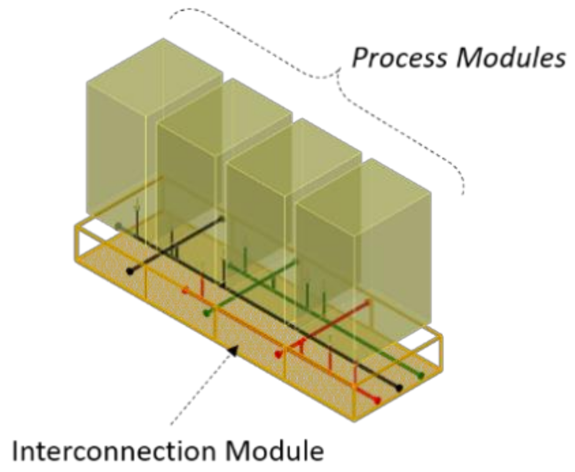
  • Interconnection module.
Figure 7 shows a 3D sketch of a possible SGB with four modules connected through a common interconnection module that contains the proper arrangement of pipes and valves to enable the interactions among the process modules installed.
The cost of the interconnection module is considered similar to a manifold system in the QUE$TOR database. Manifold costs include the structure, piles, and the pipes and valves system that are a function of the number of connections. Additionally, a subsea control unit is included for each SGB to support the functionalities of the manifold.
  • Flowlines and umbilical
Additional static and dynamic umbilical are considered when installing the first pump or compressor module. The power cable is calculated based on the power requirements, while the hydraulic line is considered proportional to the flowline dimensions and the amount of equipment connected.
The additional flow lines and risers for the second or/third phase are included when installing the first separator of each type (gas–liquid or oil–water). The characteristics and dimensions (length and inner diameter) of the lines are a copy of the original line for the multiphase fluids according to the specific location of each separator. As a simplification, the single-phase lines were not recalculated; nevertheless, futures works should include the proper pipeline designs for the single-phase streams according to the relevant standards.

2.6. Case Generation

The configuration of the SGB depends on a variable number of process modules and process train sequences or process steps. The process steps contain the order of the process modules used for a given configuration. Thus, the generation of cases is based on the permutation of all possible combinations of the process modules that satisfy a group of logical constraints. Therefore, it is possible to create a case matrix, as shown Figure 8. The matrix dimensions (N and P) are given by the N possible configurations and P process steps. Both the process modules and the process steps are divided into four branches, according to the fluid type: multiphase, oil, gas, and water. The formulation of all possibilities per branch is a function of the permutation of the process module and their operational state (on or off), as shown by Equation (9).
For example, for the multiphase flow line, there are three process modules that could be ordered in n ! possible ways, but each of these process modules could be operating or not. From Equation (9), the C a s e m u l t i p h a s e = 48 . These 48 cases represent all the possibilities, but they include impossible arrangements or cases with equivalent performances that should be removed from the final case matrix, as shown in Figure 9.
C a s e b r a n c h = n ! 2 n
The final cases matrix is built after applying the logical constraints and grouping the process steps of all the branches. These constraints should be designed only to avoid physically impossible solutions but not to discharge unusual possibilities. The objective at this point is to generate all possible solutions. Some of the constraints considered in this work include:
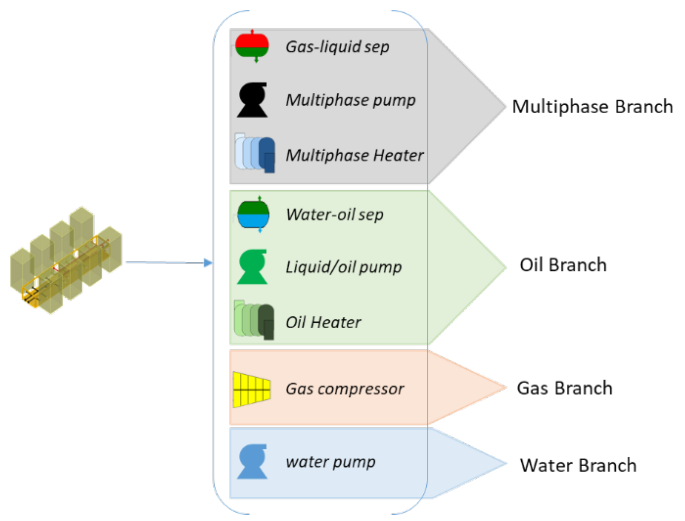
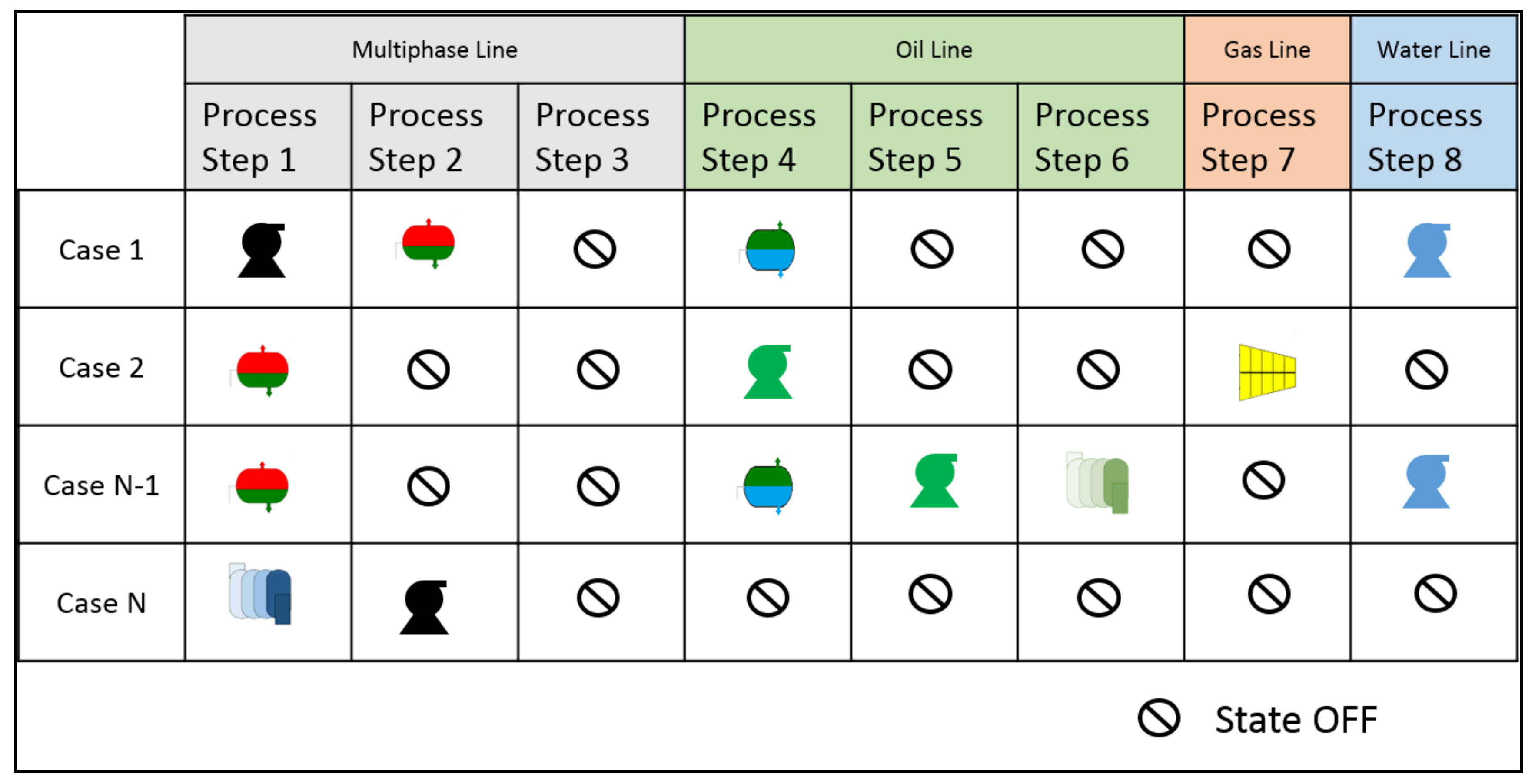
  • The oil and gas branches are enabled after a gas–liquid separator.
  • The water branch is enabled after an oil–water separator.
  • The multiphase branch becomes disabled after a separator module.
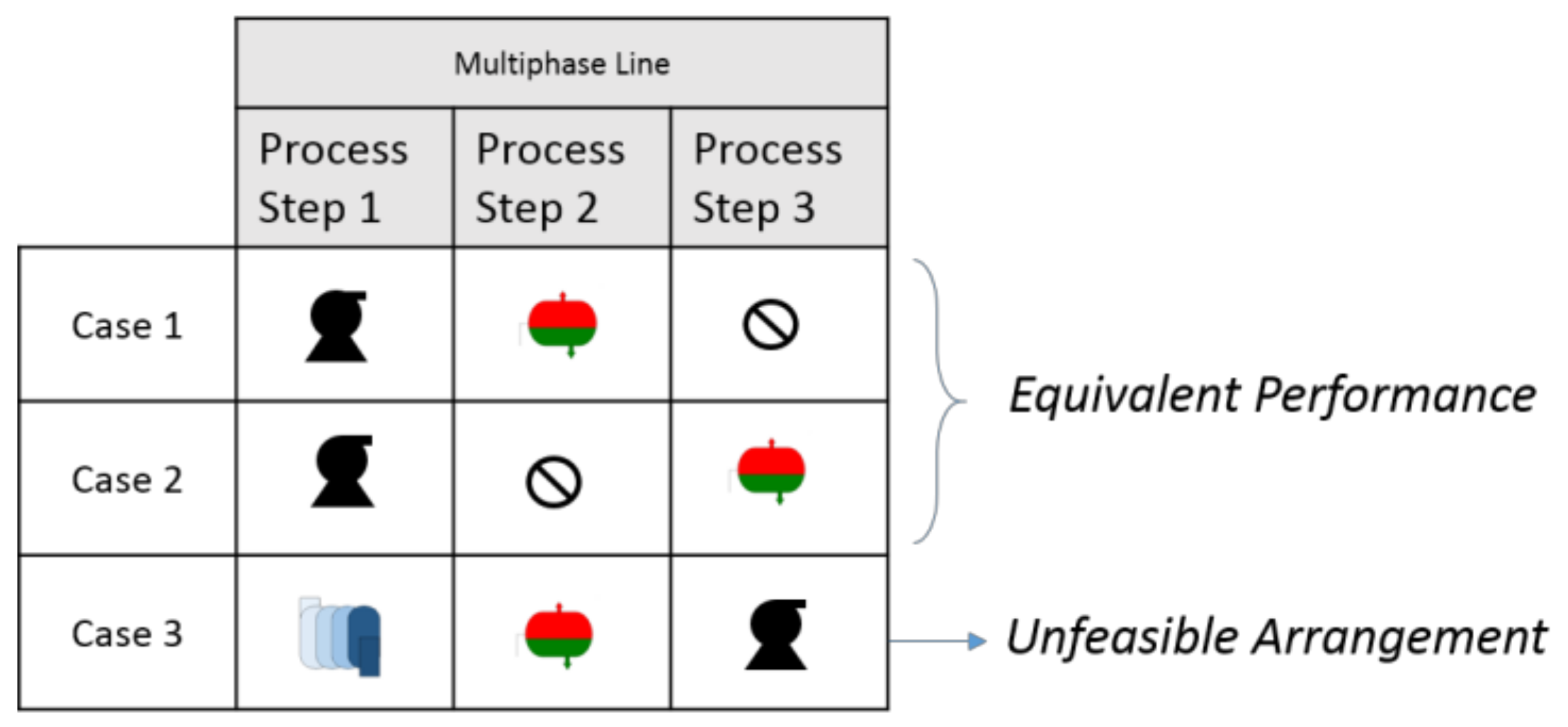
  • The removal of duplicate cases (equivalent performance).
For the process modules given in Figure 2, the configuration matrix would contain N = 275 cases. The number of boxes to install and their geographical locations would define the final architecture of the field. There is no special restriction on the locations of the SGB; they can be installed at the individual wellhead, at a given manifold or commingling point, or the riser base. Likewise, to maximize the flexibility of the solution, there is no restriction on the number of simultaneous boxes that can be installed. Since the SGB could be configured in N possible ways, the total number of possible designs of the field is given by Equation (10).
k = 1 L N k L ! k ! L k !
where k is the simultaneous number of the SGB, L is the total number of possible locations within the field, and N is the number of possible SGB configurations; this is the size of the configuration matrix in Figure 8.

2.7. Evolutionary Algorithms

Evolutionary algorithms (EA) are a subset of evolutionary computation within the artificial intelligence field. EA uses mechanisms inspired by the biological evolution theory, such as reproduction, recombination, mutation, and selection. EA have been successfully used in a variety of systems and applications, but the most important contribution to problem solving has been within the meta-heuristic optimization for large-scale problems or where analytic model-based solutions may not be suitable, including the automatic generation of test cases within software development, such as the problems presented in the contributions of [16,17,18,19,20,21,22,23,24]. The purpose of EA is to guide the search, evolving a set of solutions to satisfy the optimization problem objectives.
Six main paradigms can be considered within EA [21,38,39]:
  • Genetic Algorithms: A population of binary numbers or character strings evolve using a set of unitary and binary transformations and a selection process.
  • Evolutionary Programs: A population of data structures evolve through a set of specific transformations and a selection process.
  • Evolutionary Strategies: A population of real numbers is evolved to find the possible solutions of a numerical problem.
  • Evolutionary Programming: The population is constituted by finite state machines that are subjected to unitary transformations.
  • Differential Evolution: A direction-based search algorithm. It could be considered a real parameter-coded version of genetic algorithms, but the application and sequence of the variation operators differ with respect to the genetic algorithms and evolution strategies. The decision space is multidimensional [39].
  • Genetic Programming: The population consists of programs that solve a specific problem. The objective is to evolve the population in order to find the best program that solves the problem under study.
For the problem statement considered in this work, screening and optimization need to be performed based on the data generated by the IPM rather than the availability of explicit analytic models. The full combination of possible cases, given by Equation (10), may be very large to be able to screen completely the whole domain of scenarios in a reasonable time frame. It is therefore desirable to automate the generation of test cases and evolve a set of solutions to an optimal or near-optimal solution without the need for screening the full scenario domain. Considering the above-mentioned challenges and needs, as well as inspired by the solutions EA has provided to similar problems, the focus of this work centered on the evaluation of the suitability of EA for this application. The key features making EA a suitable candidate for this research work are the capabilities to evolve and handle large-scale optimization problems, support multiple scenario generation without the need for explicit analytic models, and the flexibility provided by the different paradigms in terms of data structures that can be used for solution encoding.
Section 2.6 and Section 2.4 describe the processes to generate a configuration matrix of the possible cases for each subsea gate box, as well as a superstructure creation. This configuration matrix will be used by the EA as the input to generate a subspace of field configuration cases, using subsea gate boxes or decentralized subsea processing modules, making them evolve to satisfy defined optimization goals, considering the relevant problem constraints. For this work, the optimization function is represented by the fitness function introduced in Section 2.5.1, and the problem constraints are mainly related to avoid solutions outside the valid domain. Additional constraints and details about constraint handling are presented in Section 2.7.3Mutation” and Section 2.7.4.

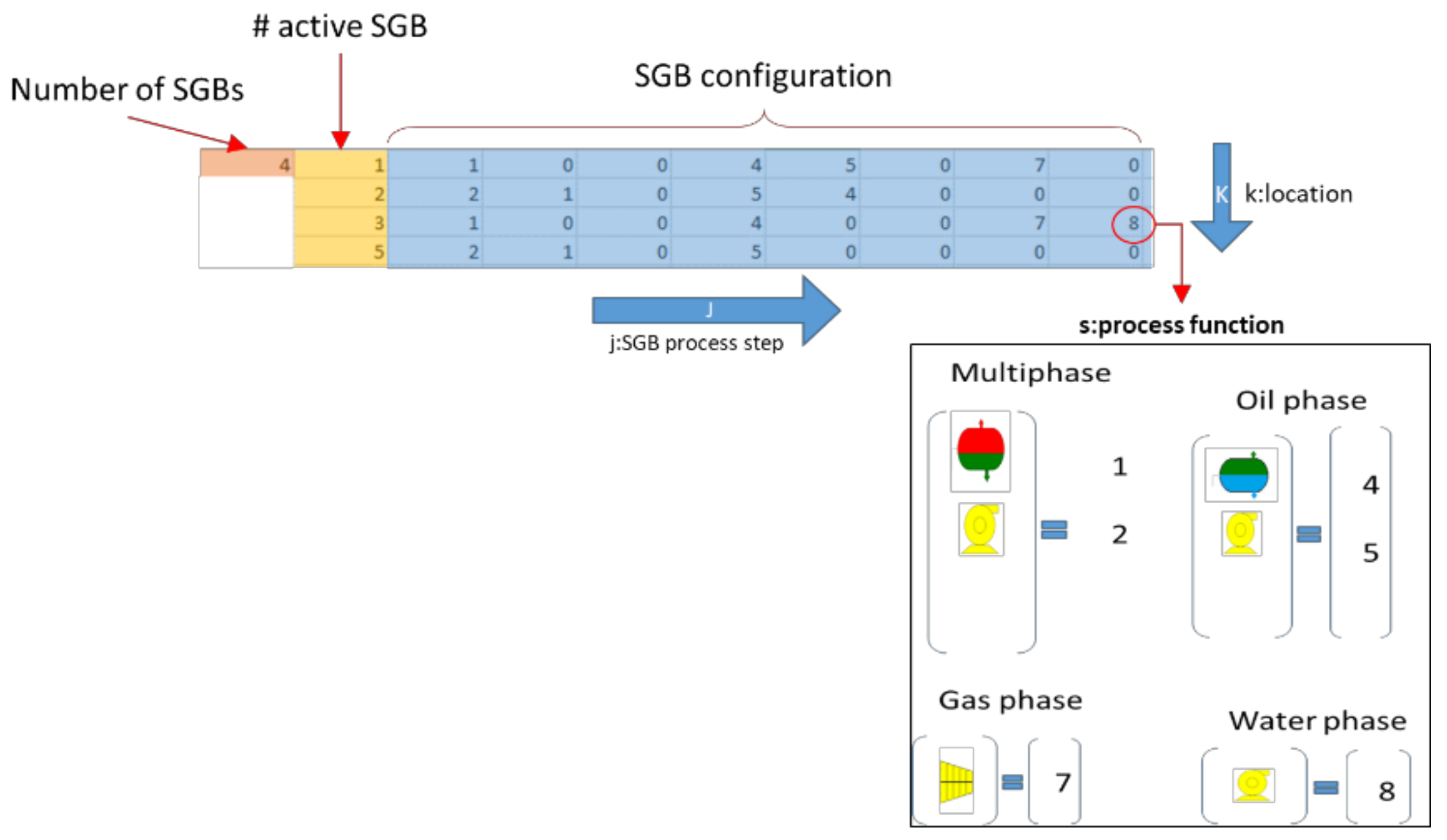
2.7.1. Individuals Encoding and Initialization

Field configuration cases/solutions, called EA individuals, are encoded as chromosomes or genotypes, C l , in terms of the arrays representing the SGB configuration cases for each possible field location, as shows Figure 10:
C i x i   =   G e n i x i   ; x i = j     I +     0
where:
  • i = 1 . . n ;   j = 0 . . m
  • n = M a x   L o c a t i o n s
  • m = M a x   S G B   c o n f i g u r a t i o n   c a s e s
  • L = 1.. N i n d
  • N i n d = N u m b e r   o f   t h e   I n d i v i d u a l s   i n   t h e   p o p u l a t i o n
Then, the population Matrix C will be constituted by the aggregation of all C l individuals with dimensions N i n d   x   n .
The position i of each gen in the chromosome represents the field location where an SGB can be placed and the gen value, allele, x i = j , encoded as a positive integer number or zero, represents the SGB configuration case at i location. Zero represents no SGB placed at the i location, respectively. The values for j can be different for each gen in the chromosome.

2.7.2. Population Initialization

Individuals/chromosomes initialization is performed by generating N i n d number of arrays with dimensions equal to n. Gene values x i are initialized using a random function with a uniform probability distribution between 0 and m. N i n d , the number of individuals, is the size of the initial population.

2.7.3. Variation Operators

Variation operators are mechanisms used to perform changes in the population during the execution of an EA [38]. There are two classic operators inspired by the biologic evolution theory: crossover and mutation. However, there are more advanced operators proposed in the literature oriented to solve specific problems, including the incorporation of other techniques [38].
Based on the encoding documented in Section 2.7.1, the problem is integer values and multidimensionality. Integer values are considered a subset of real values; therefore, evolution strategy operators can be considered at the gen level. Some of the structural operators from the genetic algorithms can also be considered at the chromosome level, since integer values are used. Differential evolution was not considered at this stage due to the differences of the applications and sequences of the main variation operators respective to the evolution strategies and genetic algorithms, but it will be evaluated later to develop further the algorithm for global optimization as a part of future works. The intention of this work is to explore the capabilities over several genetic operators and evolution strategies, as well as to identify the potential combinations or modifications required over the existing operators. The objective is to develop an algorithm to address the optimization problem related to the decentralized subsea processing module configurations and locations.
For this work, crossover and mutation operators were considered. There is a wide variety of crossover and mutation operators used for genetic algorithms and evolution strategies in the literature [21,38,39,40,41]. The variation operators considered for the evaluation and comparative analyses to verify their suitability to this application are documented in Section 2.7.3Crossover” and “Mutation”.

Crossover

Crossover is a variation operator that emulates the process of natural reproduction using simple operations over two individuals selected as parents. Crossover can be performed at the parametric level over the gene’s values or at the structural level over the chromosome segments to generate the offspring. Parametric crossover is normally used within evolution strategies, also called real-coded crossover operators [20], while structural crossover is more commonly used within genetic algorithms. The following crossover operators were considered for evaluation:
  • Parametric—Heuristic Crossover: Let C l r x be the chromosome corresponding to the lth position in the population during the rth generation: l = 1... N i n d , and let C l r x and C k r x be two individuals selected from the population as parents: k ≠ l. The crossover produces the following offspring: O l r x and O k r x [21].
    O l r x =   C l r x + α C l r x C k r x
    O k r x =   C k r x + α C k r x C l r x
    where C l r and C k r are defined as in Equation (11). Parameter α must be a very small positive number compared to the order of magnitude associated with the gene’s values of each chromosome [21]. It can be also limited to a random or fixed number between 0 and 1; depending on the application [40,41], α can be also adaptive if required. For this application, α is randomly selected with uniform probability distribution between 0 and 1.
  • Parametric—Arithmetic Crossover: Let C l r x be the chromosome corresponding to the lth position in the population during the rth generation: l = 1...Nind, and let C l r x and C k r x be two individuals selected from the population as parents: kl. The arithmetic crossover produces the following offspring: O l r x and O k r x [39].
    O l r x   =   α   C l r x + 1 α C k r x
    O k r x =   α C k r x + 1 α C l r x
    where C l r and C k r are defined as in Equation (11), and α is a random number with a uniform probability distribution between 0 and 1.
  • Parametric Average/Intermediate Crossover: Let C l r x be the chromosome corresponding to the lth position in the population during the rth generation: l = 1...Nind, and let C l r x and C k r x be two individuals selected from the population as parents: kl. The average crossover produces the following offspring O l k r x :
    O l k r x =   C l r x + C k r x   2
    where C l r x and C k r x are defined as in Equation (11). This crossover generates only one child per operation.
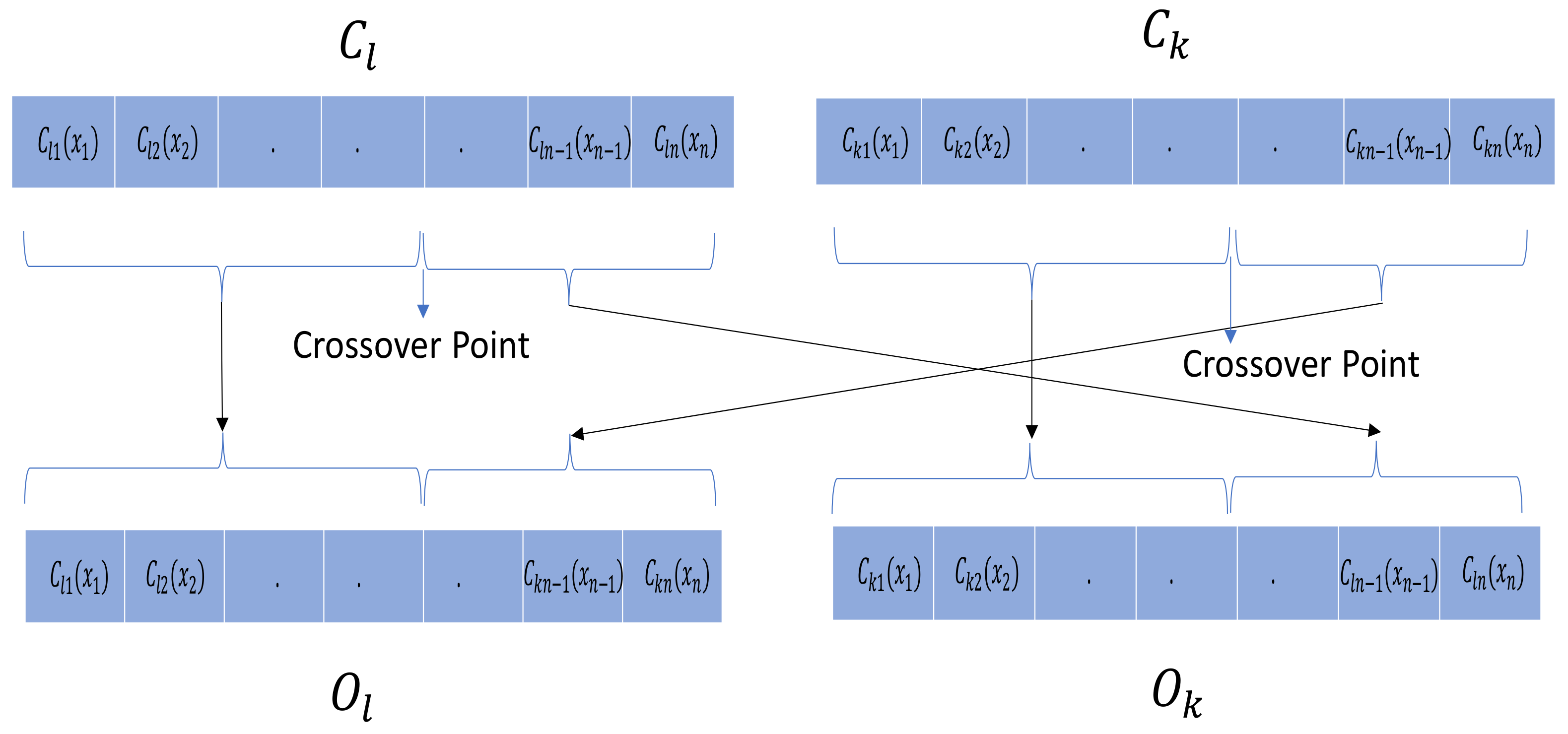
  • Structural Segmented Crossover: It is a multipoint segmentation where the numbers of the points p = 1…n−1 are variables, randomly selected, given by a segmentation probability [38]. Let C l r x be the chromosome corresponding to the lth position in the population during the rth generation: l = 1...Nind, and let C l r x and C k r x be two individuals selected from the population as parents: kl. The segmented crossover is then performed as a combination of the parents at the crossover points, producing the offspring O l r x and O k r x . Figure 11 illustrates the p = 1 point segmented crossover.
  • Structural Uniform Crossover: A uniform crossover selects the two parents C l r x and C k r x for the crossover at each generation r. It generates two offspring: O l r x and O k r x of n genes selected from both parents uniformly. Indexes l and k are positions in the r population, kl, with size Nind. Gene selection is driven by a random real number, between 0 and 1, with uniform probability distribution determining whether the first child selects the ith gen from the first or second parent [41]. The second child can be generated using the same process. Alternative solutions may also be applied to the second child, maintaining a uniform selection. For this specific application, the alternative solution applied to generate the second child was mirroring the parent genes not selected for the first child. Let C l r x and C k r x be two individuals selected from the population as parents: kl. The structural uniform crossover produces the offspring O l r x and O k r ( x ), where O l r x is produced using a random uniform probability distribution to decide the selection of the parent genes, and the second child O k r ( x ) may be generated using the same random process or, alternatively, using the opposite selection with respect to the first child ¬ O l r x , as illustrated in Figure 12, where ¬ O l r x contains the gens not selected for O l r x . Then, O k r ( x ) = ¬ O l r x .
  • Crossover Rate: The crossover rate or crossover probability defines the number of times a crossover operation occurs for chromosomes in one generation. The crossover rate is defined as a real number between 0 and 1. Different selection approaches can be applied depending on the application; they can be random, fixed, or adaptive. The authors of [42] presented a review on this topic including a dynamic approach. Adaptive and deterministic control methods for the crossover rate were also presented in [39]. For this application, the crossover rate was fixed set to 1 in order to maximize the number of solutions to be processed further within the EA without having the need to increase the population size prior to the crossing step. More details about the combined process within the proposed EA in this paper are documented in Section 2.7.10 and Section 3.

Mutation

A mutation is a variation operator that emulates the evolutionary process of changing the genetic structure of a species to be able to adapt and to maintain diversity [38]. It is equivalent to a biological mutation. A mutation is performed by modifying one or more genes values in a chromosome from its initial state. The following mutation operators used mainly within evolution strategies were considered for evaluation:
  • Boundary Mutation: This mutation operator replaces the genome with either a lower or upper bound randomly [39]. An alternative option, and the one used in this paper, is to replace the genome-containing values outside of the feasible domain boundaries with a random number uniformly distributed within the boundaries [L-U], where L is the lower boundary value and U is the upper boundary value. This is very useful for constrained optimization. Both approaches can be used for integer and float genes.
  • Normal Mutation: A normal distribution disturbance N μ , σ 2 is performed on one or more genes of a chromosome, where μ is the mean and σ the standard deviation. The normal distribution disturbance with μ = 0 can be written as σ N 0 , 1 [39]. The standard deviation σ can be fixed, random, or adaptive. The authors of [39] presented a review on normal mutation control parameters. Let C l r x be the chromosome corresponding to the lth position in the population during the rth generation: l = 1...Nind, where each gen is defined as per Equation (11).
    The mutant C ˜ l r x generated from C l r x using a normal mutation can be written as follows:
    C ˜ l r x   =   C l r x +   σ N 0 , 1
  • Gradient Mutation: The gradient mutation is performed on one or more genes for a chromosome along a weighted gradient direction of the fitness function based on the algorithm originally proposed by [43] for nonlinear programming problems and adapted to be part of an evolutionary algorithm for linear systems identification in [21]. This mutation is oriented to maximize the fitness function f(x) using penalty functions of the type g x 0 as constraints to penalize solutions out of the feasible domain, where x represents an individual of the population in the original algorithm. As the number of generations increases, the individuals/solutions with less fitness function value, as well as the nonfeasible solutions, will die gradually, and the fitness function is expected to reach the optimum or near-optimum value. A convergence analysis of this algorithm was presented in [43].
    To be consistent with the nomenclature defined for this application, as per Equation (11), let C l r x be an individual/chromosome corresponding to the lth position in the population, during the rth generation: l = 1... N i n d , where each gen is defined as per Equation (11). Let f( C l r x ) and g( C l r x ) be the fitness function and penalty function, respectively; then, the total gradient direction d C l r x   is defined as:
    d C l r x   = Δ f C l r x   s = 1 S ρ s Δ g s C l r x
    Given the nature and complexity of this application, the gradient directions for f( C l r x ) and g( C l r x ) are calculated as finite differences of the fitness and penalty functions between the two consecutive generations and, therefore, defined as Δ f C l r x   and Δ g s C l r x , respectively, where S is the total number of penalty functions or constraints associated with the problem, and ρ s are penalty function multipliers acting as the weights of the gradient direction, given by
    ρ s = 0 g s 0 δ s g s > 0
    δ s = 1 g m a x C l r x g s C l r x + δ
    g m a x x = M a x g s x ,   s = 1 S
    where δ will be a very small positive number.
    The mutant C ˜ l r x , generated from C l r x , along the weighted gradient direction d C l r x   , can be defined as:
    C ˜ l r x = C l r x +   β   d C l r x
    For the original algorithm presented in [43], β is a step length of the Erlang distribution random number with declining means generated by a random number generator. For the Systems Identification application presented in [21], β is a very small number compared to the order of magnitude associated with the individual gens adjusted to suit the specific applications. For the optimization problem presented in this paper, the gradient mutation was applied, tailoring a parameter control strategy to suit this problem statement. The application-specific details are described in the following subsections.
  • Application Specific Gradient Mutation Penalization Functions:
    The following penalization functions were defined for this application:
    g 1 = M a x C l r x m   0
    where m is the maximum number of feasible subsea gate box (SGB)/decentralized process module configuration cases, as defined in Equation (11).
    g 2 = M i n C l r x 0
    The above Equations (23) and (24) penalize solutions outside the feasible domain, having chromosome values greater than m or the negative.
    For this application and encoding, there is a risk of obtaining repeated solutions that have been evaluated and discarded; this can add unnecessary computational time within the EA, as well as additional IPM model simulation time, processing repeated solutions. In order to reduce this risk and maximize the exploration and diversity, all previous solutions that have been subjected to an evaluation in the previous (r−1)th generations are registered in an ancestors matrix: A r 1 . Then, a third penalization function is defined as g 3   0 , where
    g 3 = 1 C l r x     A r 1 0 o t h e r w i s e
    See more details regarding the ancestors matrix in Section 2.7.5.
  • Application Specific Gradient Mutation Parameters Control: After the preliminary analysis and evaluation of gradient directions and penalization functions profiles, the need for defining the δ and β parameters became apparent to control the order of magnitude of g( C l r x ) and the weighted gradient direction contributions β   d C l r x   with a different strategy, as originally defined in [21,43]. The parameters’ control for this application is dependent on the nature of the crossover operator used before mutation. Various scaling and normalization methods for the fitness and penalization functions were tested before to solve this issue without success; therefore, it was decided to define these parameters dynamically or statically, depending on the crossover operator being used. A heuristic crossover, for example, may generate solutions out of the feasible domain, and therefore, it may produce large values of the penalization functions g( C l r x ) during the first generation. Very small values of δ below 0.1 may produce large penalization multipliers and, therefore, large, weighted variations in the mutation, reducing the performance of the gradient contribution. For the rest of the crossover operators listed in this section, this does not occur. Therefore, when using a heuristic crossover operator before gradient mutation, selecting values of δ between 0.1 and 0.5 is appropriate for this application.
    On the other hand, when using the structural uniform crossover, no solutions outside the feasible domain are generated, and therefore, g 3 will be the only penalization function that can be activated. For this case, calculating δ is proposed based on the inverse average gradient direction of the fitness function for all individuals in the population at each r th generation as follows:
    δ = 1 2 m e a n Δ f C l r x + 1 = N i n d 2 l = 1 N i n d Δ f C l r x +   N i n d
    where N i n d is the total number of individuals, as defined in Section 2.7.2. This allows controlling the magnitude order of the weighted gradient direction d C l r x       l by controlling the amplitude of the penalization functions based on the average fitness function gradient direction, while keeping 0 < δ   1 .
    Parameter β performs better starting with small values when the gradient is large, increasing proportionally to the generation number to avoid a vanishing gradient contribution when the gradient decreases with the number of generations while approaching to an optimal or near-optimal solution. The following calculations are proposed to control β , keeping 0 < β 1 :
    β = i N G A R       1   i     N G A R 1 O t h e r w i s e
    where N G A R corresponds to the generation number when the solution is expected to enter an attraction region where the optimum or a near-optimum is located. N G A R   N G m a x , where N G m a x corresponds to the maximum number of generations given as one of the termination criteria in Section 2.7.9. N G A R is a parameter that can be fixed or adaptive. Based on all sensitivities performed, the majority of the qualifying cases reached the attraction region at the 20 th generation, on average. Therefore, N G A R = 20 was used for the associated cases, and the results are presented in Section 3.
  • Mutation Rate: The mutation rate or mutation probability defines the number of times a mutation operation occurs for chromosomes in one generation. The mutation rate is defined as a real number between 0 and 1. Different selection approaches can be applied depending on the application; they can be random, fixed, or adaptive. The authors of [42] presented a review on this topic, including a dynamic approach. Adaptive and deterministic control methods for the mutation rate were also presented in [39]. For this application, two types of mutation rates were applied: one at the population level and one at the chromosome level. The one at the population level was tested for some cases with a mutation rate of 0.5, where the mutants were selected from the total, including only the offspring coming from the crossover process before the mutation. The mutation rate at the chromosome level is defined with two different random parameters, one determining the number of genes to be mutated and the second to determine the positions of the gens where the mutation will occur. The mutation rate can then be applied to the whole chromosome or to a part of it, depending on the parameter values. The parameters are chosen with a uniform probability distribution.

2.7.4. Filtration

This is an application-specific operator introduced for this work to avoid the re-evaluation of repeated solutions already evaluated in previous generations that may result from crossover or mutation operations. This filter is only applied to individuals produced as a result of the variation operators and not to the original population in the current generation. The objective is to avoid the IPM evaluating repeated solutions. It also allows that ancestors that may be fitter than the offspring or mutants produced during the current generation can survive to continue contributing with their genetic information in future generations.
Let A r 1 be an ancestor matrix that registers all solutions that were the subject of the evaluation process until the previous r 1 th generations. The filter will then determine the new solutions that qualify to be evaluated at the current generation r to be potential ancestors in the next generation:
F r = C x r M r A r 1
where C x r and M r are matrices containing the individuals produced as a result of the crossover and mutation operations, respectively. N C x , N M , and N F are the number of individuals contained in the C x r ,   M r , and F r matrices, respectively.

2.7.5. Registration of New Individuals in the Ancestors Matrix

This is a complementary application-specific operator introduced for this work to promote the ancestor’s diversity and avoid repeated and potentially discarded solutions to be re-evaluated in the IPM and processed in the EA.
Let A r 1 be an ancestors matrix that registers all solutions that were the subject of the evaluation process during the previous r 1 th generations and F r the matrix containing the new individual results of the filter applied in the r th generated, as described in Section 2.7.4. The update of the ancestors matrix for the r th generation is performed by registering the new individuals not previously registered.
A r = A r 1       F r   r > 1
For the first generation, the initial population C 1 will be directly registered in the ancestor matrix:
A 1 = C 1

2.7.6. Evaluation

The actual evaluation process of the new individuals is performed as follows:
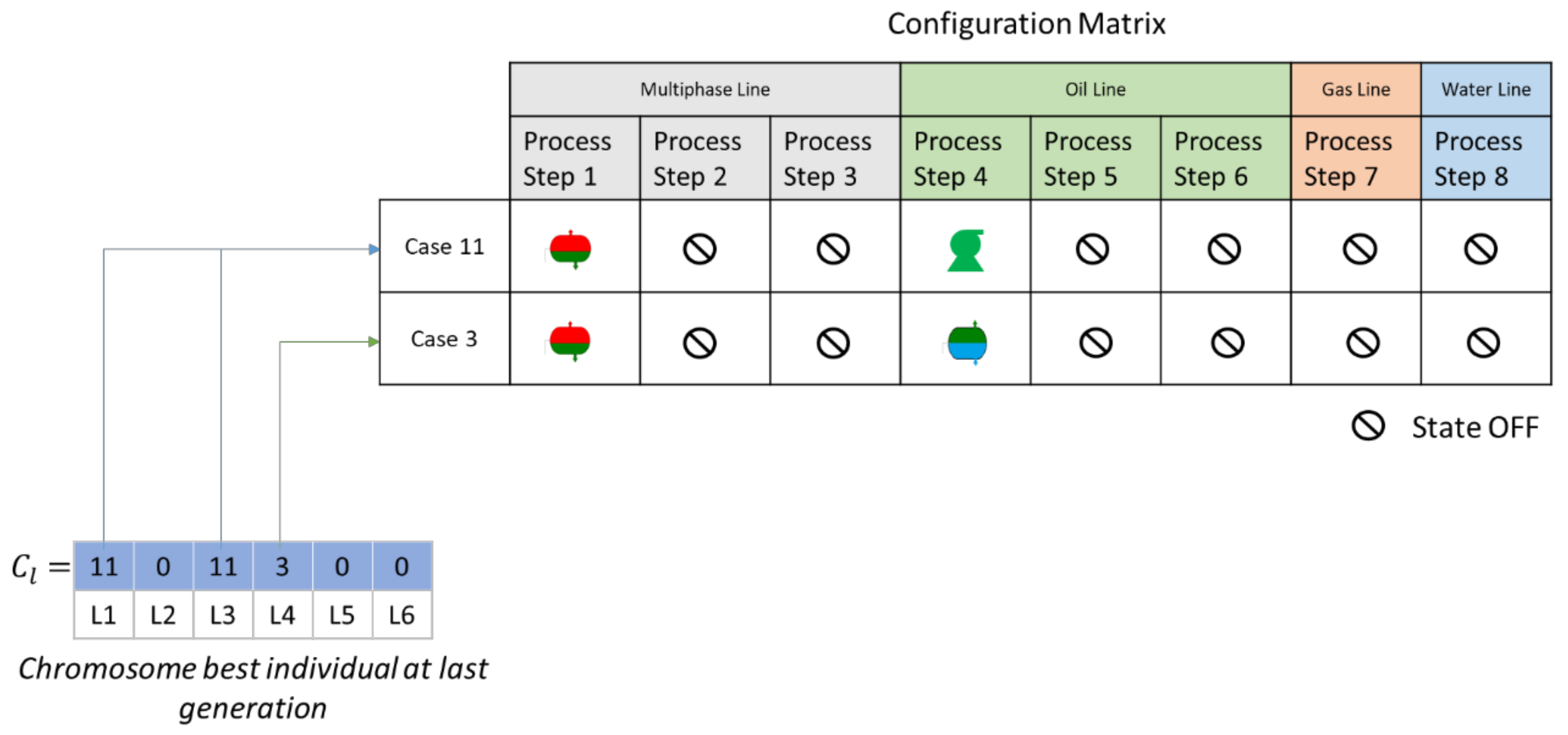
  • Decoding of the chromosome structures into decentralized processing module configurations for the field.
  • Reconfiguration of the superstructure integrated into the IPM with the decoded configuration from the EA.
  • Run the IPM with the decoded configurations for the expected field life.
  • Calculate the fitness function value based on the production potential obtained from the IPM, the development cost CAPEX, and the expected OPEX associated with the decoded configuration, as documented in Section 2.5.1.
  • Transfer the fitness function value to the EA to continue the selection and ranking process, as documented in Section 2.7.7 and Section 2.7.8 as well as illustrated in Section 2.7.10.

2.7.7. Selection

Selection processes are mechanisms used for different purposes within an EA in order to:
  • Conform the number of individuals or parents that will participate in the reproduction process.
  • Control the population management, survivor’s selection, individual’s elimination, and/or replacement.
  • Select the best individuals that satisfy the objectives to an optimization problem.
Selection mechanisms are important to support the EA reaching an optimal solution, as they grant fitter individuals a higher opportunity of propagating their high-quality genes [39]; however, the identification of an ideal selection mechanism is not always straightforward. There are multiple selection mechanisms documented in the literature varying from traditional methods to specific applications. Reviews of some of these mechanisms can be found in [38,39]. For this application, two simple rank-based selection methods are applied:
  • Direct fitness rank-based selection: This method sorts the individuals from the highest to the lowest fitness values. This ranking is used to:
    -
    manage the population size by selecting the number of fittest individuals to continue to the next generation.
    -
    monitor and select the best individuals that satisfy the optimization objectives to control the termination criteria.
    -
    prioritize the set of parents that will be crossed based on their fitness values. This method may prematurely accelerate the convergence of the algorithm to a local attraction region.
  • Direct fitness + gradient rank – based selection: This method sorts the individuals from the highest to the lowest fitness + gradient values. This is only used as an option to prioritize the set of parents that will be crossed based on their combined fitness + gradient values when the gradient mutation is used. This selection method was introduced for this specific application to avoid premature convergence of the algorithm to a suboptimal attraction region and keep the gradient energy, as well as continue exploring the solutions space as long as possible. This mechanism may deaccelerate the convergence speed but may increase the exploration capabilities and discovery of new solutions.

2.7.8. Replacement

Replacement mechanisms are normally used to keep the population size constant, which is the case applied in this paper. There are several replacement mechanisms reported in the literature. A review of some of these methods can be found in [38,39].
The method used in this paper can be defined as direct fitness ranked and inclusion-based replacement. This method includes the Nind individuals contained in the original population matrix C r for a given generation r and the new N F individuals resulting from the filtration process contained in the matrix F r , as described in Section 2.7.4.
The total of the individuals N T = Nind + N F     N F > 0 is subjected to a direct fitness ranked-based selection process, as defined in Section 2.7.7. After the ranking is performed, the best new Nind individuals are selected from the total N T for continuing to the next generation. The rest of the individuals are eliminated to keep the population size constant.
C r + 1 = N i n d   I n d i v i d u a l s   w i t h   M a x   F i t n e s s   F u n c t i o n f r o m   C r   F r     r 1
This replacement process guarantees the survival of any ancestor in the C r fittest than the new individuals in F r .

2.7.9. Termination/Stop Criteria

There are different categories of stop criteria often used within EA. Some of them are documented in [39]. For this application, the stop criteria will be activated if a maximum number of generations N G m a x is reached or if the fittest quarter of the population has not evolved during the last 5 generations. For this application, N G m a x = 50 proved to be enough as the maximum number of generations. The results and analysis details are documented in Section 3.

2.7.10. Proposed Evolutionary Algorithm Flow Diagram

For the test set-up to support the evaluation for this study, the variation operators described in the previous sections were combined and tested, as illustrated in Figure 13. Two mutation mechanisms in a series were proposed. The first can be either a normal mutation or gradient mutation followed by a boundary mutation mechanism. More details on the test set-up, evaluation, analysis, and results are documented in Section 3.

2.8. Business Case

A preliminary study of the subsea gate box was performed in [1]. For this first stage of the study, the authors used a simplified version of a subsea gate box that only considered modular multiphase pumps. Thus, for a synthetic business case, the authors compared the production profile and cumulative production for a different number of pumps installed at different locations along the field and working according to two different operational philosophies. The objective of the business case was to improve the production performance of a target well within the field. Using an integrated reservoir-network model, [1] showed the possibility to increase production with the modular concept of the subsea gate box by 24% for the target well and 6% for the entire field respective to the central boosting station.
For the present work, the same synthetic field considered in [1] was used, but extend the numbers and types of processes that can be installed within the subsea gate box. The business case is a subsea production system that includes two oil fields: Field A and Field B. Field A is considered the main field, while Field B is a remote field located far away from the main topside facility. Each field contains three satellite wells connected to a common manifold at each field (Manifold A and Manifold B, respectively). The two manifolds are connected in a series, and the total production of the two fields is conveyed through a single S-riser towards the topside facility. The receiving separator is 30 bar, while the initial reservoir pressure is about 360 bara in Field A and 276.8 bara in Field B [1].
The business case from [1] was simplified to facilitate the performance evaluation of the EA implemented in the methodology. Therefore, the production constraints and internal optimizations of the IPM were disabled. Furthermore, the process unit settings were kept constant throughout the production period regardless of the theoretic performance of the typical equipment.
The concept screening for this business case considers the potential application of the subsea gate box concept for improving the performance and production of the field. The objective of this exercise is to outline the best scenario that maximizes the revenues of the project. The final scenario is defined by the number of SGB required, their internal configuration, and the geographical location of each SGB.
For the business case proposed, there are six possible geographical locations to install a SGB, as is shown in Figure 14. Furthermore, the SGB internal configuration considers six possible processing units: multiphase boosting, gas–liquid separation, oil–water separation, oil boosting, water boosting, and gas compression. For these six types of processes, there are 33 possible configurations for a given SGB. Combining all possibilities of the SGB number and configuration located at any combination of all suitable geographical locations, the search domain is about 1.5 × 10⁹ possible scenarios.

3. Results

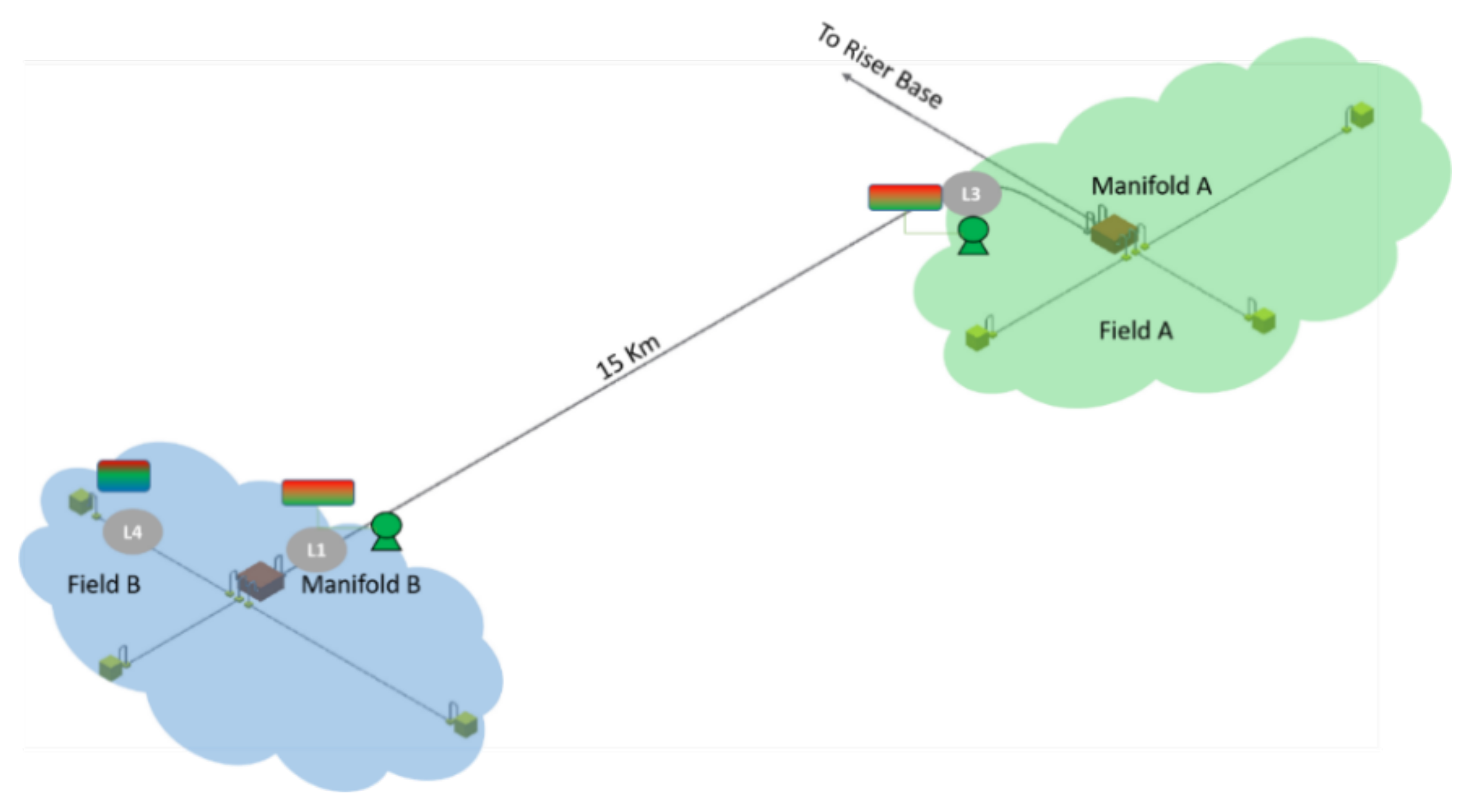
3.1. Field Concept Selection for the Business Case

After executing the methodology proposed in Figure 3, the outcome of the algorithm will offer the near-optimal scenario for the field architecture provided and the operating conditions stated within the IPM model. The scope of the solution is to provide the arrangement of the decentralized processing systems that enable the highest economic value of the project according to the economic parameters established.
The expected solution contains information on the principal design parameters stated in Section 2.1. The characteristics of a given individual are given by its genotype (the chromosome) and its phenotype (number of boxes, locations, and configuration). Figure 15 shows the solution for the business case presented in Section 2.8. The solution is given by the chromosome of the best individual at the last generation, which is decoded using the configuration matrix to define the corresponding arrangement of the SGB. Figure 16 corresponds to the final configuration of the SGBs after decoding the chromosome in the IPM.
The final solution suggests the installation of three boxes at locations L1, L3, and L4. Both the SGBs in L1 and L3 require a gas–liquid separator followed by a liquid booster, while the SGB in L4 requires a three-phase separator. The proposed field architecture gives a fitness value of 714.5 mill USD. The final fitness value is transduced as a differential NPV with respect to the original project profit. This means that positive fitness values represent an increase and negative fitness values represent a reduction with respect to the original project profit introduced by the required modifications to the field of architecture based on the EA results. The solution for the business case is summarized in Table 6 according to the problem specification parameters provided in Section 2.1
The solution was achieved after about 1162 evaluations and around 28 iterations (or generations). Figure 17 shows the evolution of the fitness function throughout the different generations, while Figure 18 compares the characteristics of the individuals of the initial population (original generation) with the final generation. From Figure 17, the capacity of the algorithm to evolve from an initial random configuration towards an optimal or near-optimal fitness value is visible. The entire population evolves, and all individuals change during the evolution process. The mean value by generation expresses how the average of the fitness function changes along the generation axis. The variation is sharp at the beginning of the evolution process, and it becomes flatter after a few generations when the differences among the individuals are very small. The final solution is given by the evolution of the best individual across all the generations. The algorithm shows the capability to find several individuals with higher fitness values than the original population. Furthermore, the capability of the algorithm is not limited to a positive fitness value as an initial condition for a given individual; the evolution is also evident for the worst individual of the generation, where a negative fitness value is also able to evolve towards a much higher fitness value.
A sensitivity analysis of the different parameters was carried out, aiming to evaluate the algorithm performance. After running all sensitivity cases, it was possible to evaluate about 70,951 configuration scenarios out of the total domain with 1.5 × 10⁹ possibilities. The higher fitness value registered during the sensitivity analysis was about 714.5 mill USD. Given the metaheuristic nature of this algorithm, it is not possible, at this stage, to demonstrate formally that the best-achieved solution represents the global optimum. Therefore, the best-known fitness value (BKV) can be considered a near-optimum solution.

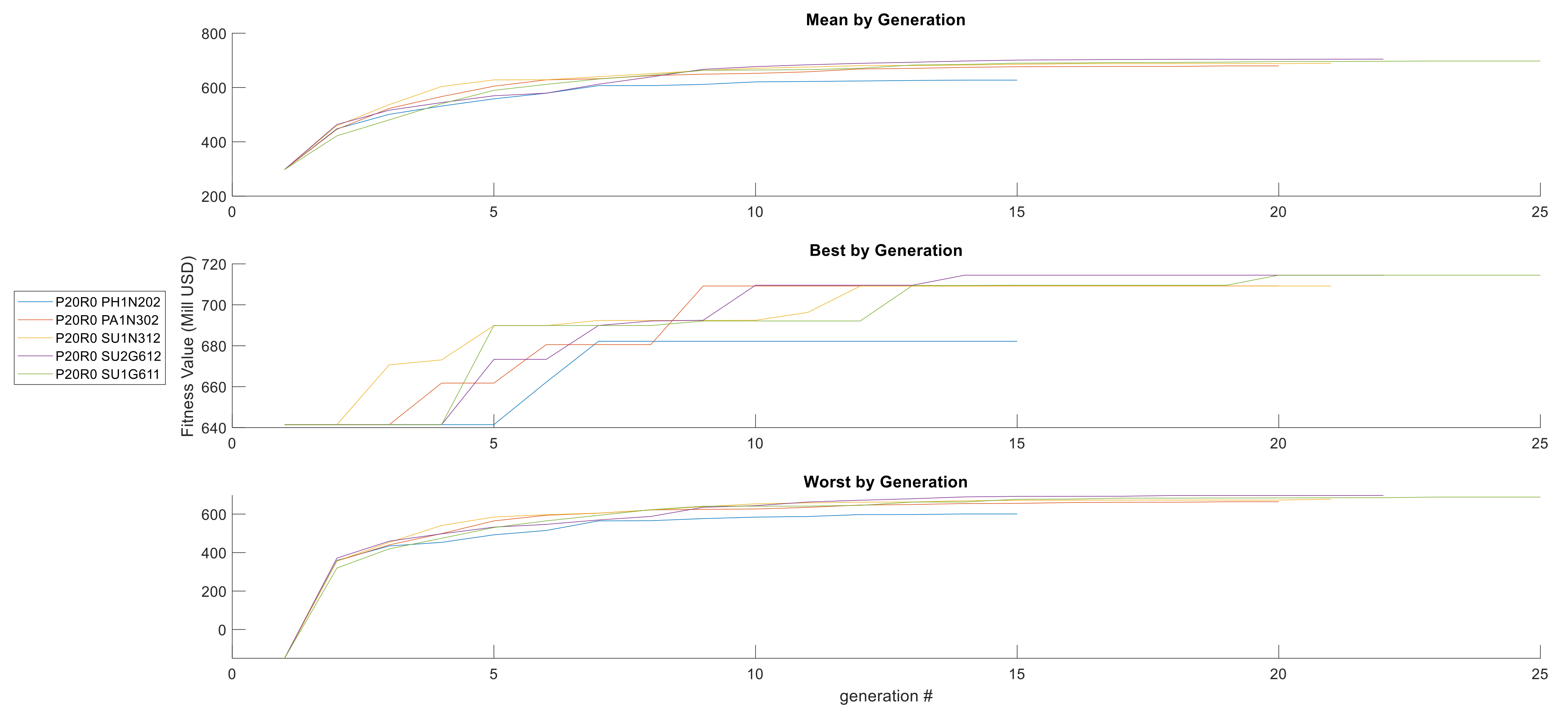
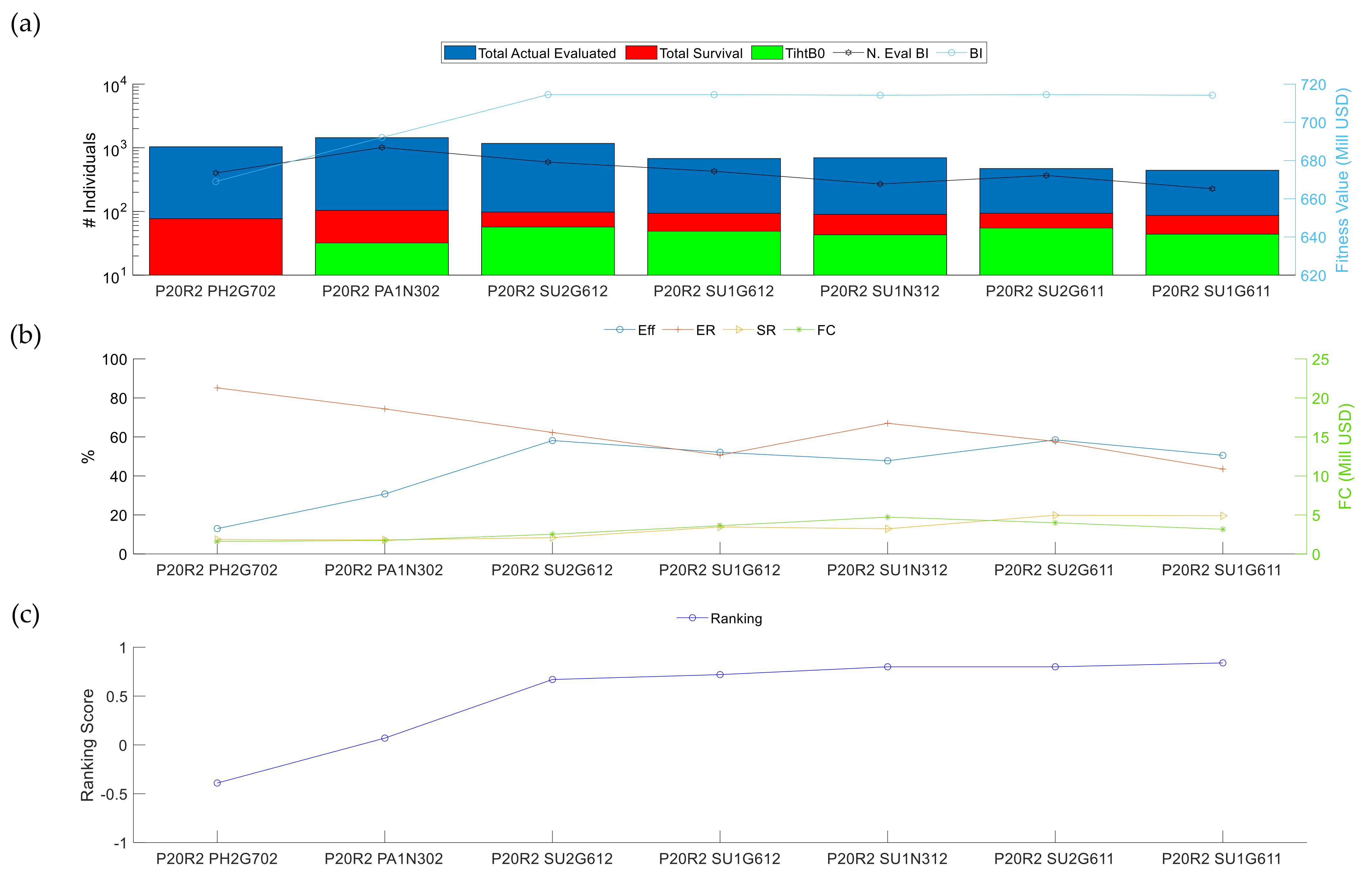
3.2. Evolutionary Algorithm Performance

The following section presents the evaluation of the EA performance as a support tool for the concept screening and optimization of the field architecture when decentralized subsea processing solutions are considered. The analysis was divided into three stages: performance of the variation operators, the impact of the initial population (initial conditions), and repeatability of the results. Throughout the analysis, the cases evaluated were identified following the codification system shown in Table 7, which are according to the sensitivity variables defined for each type of analysis. The sensitivity variables correspond to the parameters of the EA that were considered during the algorithm design for this application, which included the population size, the formulation of the variation operators (both crossover and mutation), the parent selection method, and the different levels of the mutation rate (chromosome level and population level). Each combination of the sensitivity variables of Table 7 conforms a case analysis that is identified by a tag of 12 characters given by the codification assigned at each sensitivity variable, as shown in Figure 19.
The final evaluation and comparison among the different cases is performed based on the key performance indicators (KPI) defined to rank the different EA solutions obtained, as shown in the evaluation matrix presented in Table 8. Each indicator in Table 8 is normalized in terms of the maximum and minimum values of the parameters evaluated. Then, a weighting percentage is assigned to calculate the final score of the ranking criterion.
Where:
1.
Fitness value of the best individual.
This is given by the highest value of the fitness functions for all generations. The higher the value, the higher the score in the ranking.
Since it is not possible to assure whether the BKV is indeed the global optimum solution, the rest of the analysis will be carried out considering an attraction region where the optimum or near-optimum is located. The region of attraction is defined as a region with one standard deviation of the BKV. The minimum value of this indicator is the lower limit of the attraction region as shown in Equation (32); therefore, cases that do not reach the attraction region register a negative score for this indicator. For the business case used as the example for this work, the lower limit of the attraction region is 694.6 mill USD.
F N B I = x 694.6 max X 694.6
where F N B I is the normalization of the fitness value for the best individual (BI), x is the fitness value of the best individual at the end of the simulation, and X is the vector of x of all cases evaluated for a given population.
2.
Inverse of the number of evaluations performed before finding the best individual.
This indicates how many individuals were evaluated before finding the best individual. This parameter is a measure of how fast the algorithm converges on the best solution; therefore, the lower the number of evaluations, the higher the score in the ranking.
3.
Evaluation rate.
The total number of evaluations may differ for each operator, either because of the random nature of the variables within the operator itself or due to the type of operation being used. In any case, there is a possibility to have individuals already evaluated in previous generations after the mutation and before the filter. Therefore, the total number of new individuals is reduced during the filtration process before proceeding to the evaluation stage. This performance indicator allows tracking how effective the operators are at producing new valid solutions that satisfy the boundary conditions. The evaluation rate is calculated following Equation (33). For this indicator, the higher the value, the higher the score in the ranking.
Evaluation   rate = Total   Actual   Evaluations Total   Theoretical   Evaluations 100
where the Total Theoretical Evaluations are the total new individuals, while the Total Actual Evaluations are the new individuals that satisfy the constraint criteria after the filtration process.
4.
Survival rate.
This indicator measures the ratio of the number of new individuals that survive at least one generation with respect to the actual number of evaluations. The new individuals for a given generation are defined as the individuals created by the crossover and mutation operator. The term “survival” refers to those new individuals that “survive” the selection stage to become the parents for the next generation.
Depending on the mutation rates and the constraint conditions, the total number of evaluations can vary for each operator, as mentioned in point 3. For the first generations, it is easier to find new individuals that satisfy the constraint conditions, evolving relatively fast. Nevertheless, after some generations, it becomes more difficult to create new individuals that both satisfy the constraint conditions and that are better qualified than their ancestors. As the survival rate declines, the population diversity decreases, and the evolution slows down until the generation reaches the stop criteria. For this indicator, the higher the value, the higher the ranking.
Survival   rate = Total   Survivors Total   Actual   Evaluations 100
5.
Effectiveness.
It is the measure of how many good individuals are generated by the operators and the set of parameters applied. It is estimated by Equation (35), where T i h t B 0 is determined by calculating the number of survivors (from the previous indicator) with a fitness value higher than the best individual of the initial conditions.
Although the whole generation (on average) might evolve toward higher fitness values, it is the individual with the highest fitness value that has the potential to converge on the optimal solution. The survival rate is an indicator of how efficient the exploration process is. The effectiveness, on the other hand, is a measure of the quality of those survivors. For this indicator, the higher the value, the higher the ranking.
Effectiveness   = T i h t B 0 Total   Survivors 100
where
TihtB0: Total   indv   higher   than   best   individual   in   G 0
G0: Initial Population
6.
Fitness Change (FC).
This indicator is designed to measure the evolution energy in terms of the fitness value changes of the best individual in the population per generation, as shown in Equation (36). The indicator reflects the average change of the best individual per generation. For this indicator, the higher the value, the higher the ranking.
F C = f ( C l = 1 r = N g e n ) f C l = 1 r = 0 N g e n
where   f C l r is the fitness value of the individual “l” at the generation “r”, and where l = 1 is the best individual of the populations, with the highest fitness value. This position is assigned after the fittest selection process for each generation.
7.
Inverse of the Total Number of Evaluations.
The indicator takes into consideration the total number of evaluations at the end of the study. The best performance is given by a balance between satisfying the previous indicators and performing the fewest evaluations as possible. The objective of this parameter is to include a penalization for performing too many evaluations, which is necessary when comparing cases with different population sizes or cases with similar performances. For this indicator, the lower the number of evaluations, the higher the ranking. Therefore, the indicator is the inverse of the number of evaluations (1/TE).

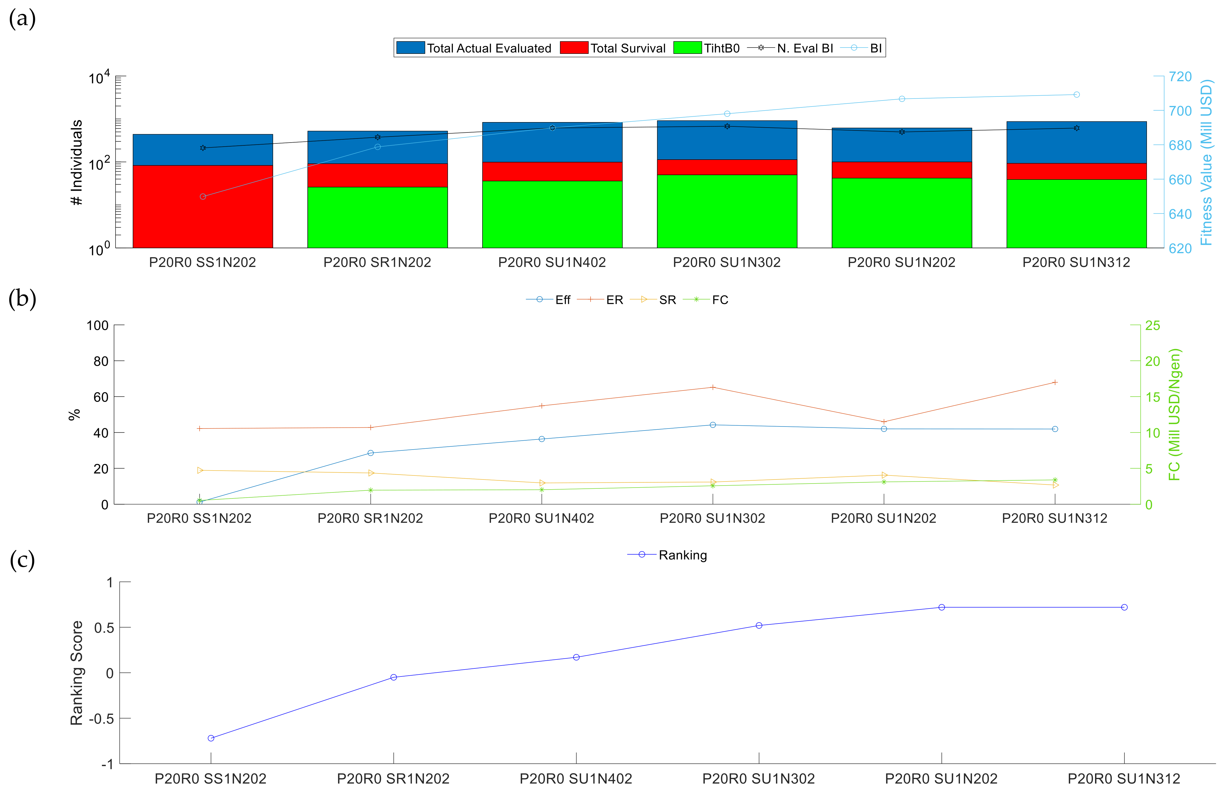
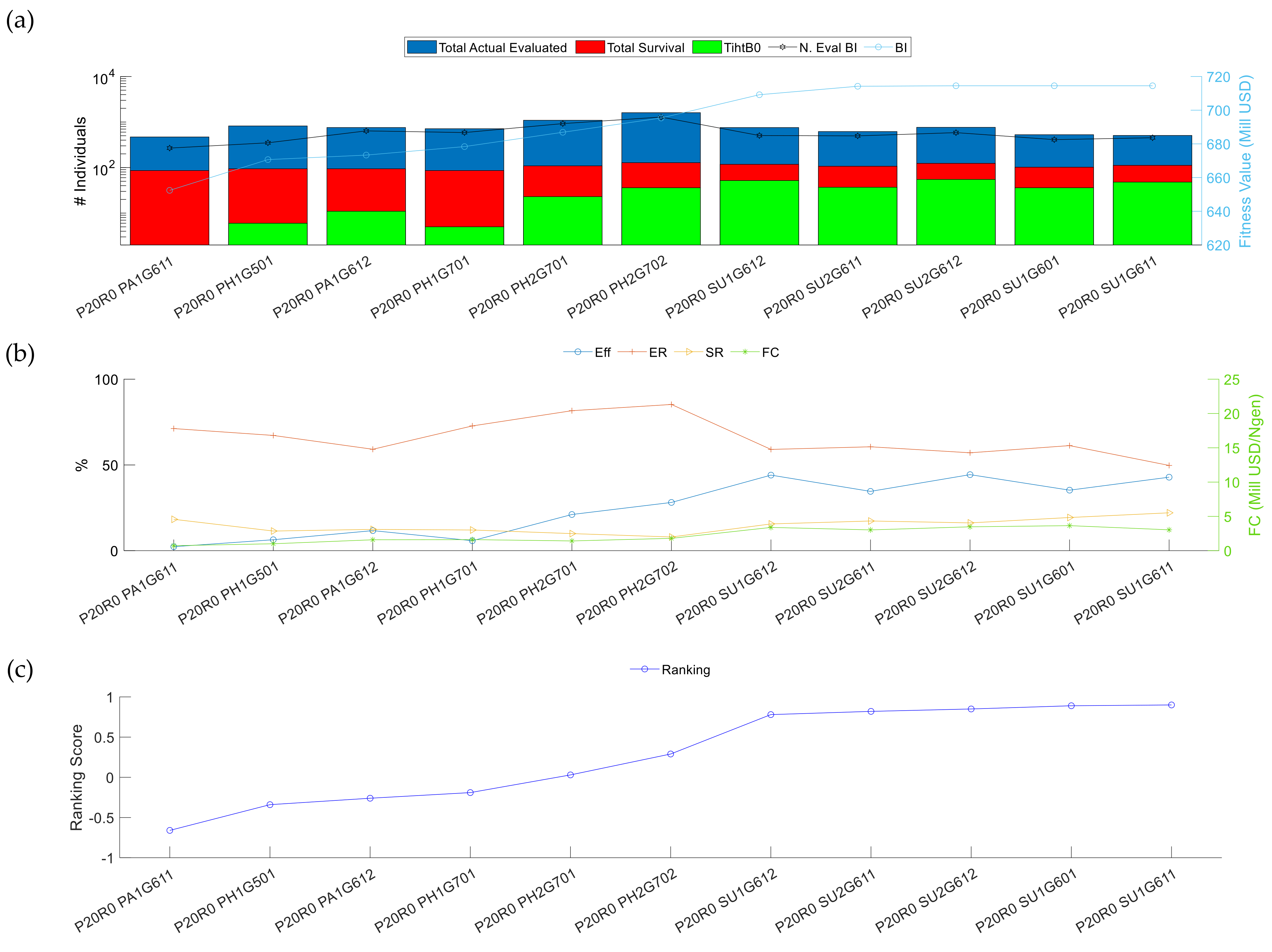
3.2.1. Analysis I: Performance of the Variation Operators

The objective is to identify the most suitable combination of crossover and mutation operators to obtain the best evolution of the initial population towards the optimal or near-optimal solution. For this first analysis, an initial population of 20 individuals (P20R0) is created randomly with a uniform probability distribution, and it remains constant throughout the analysis to evaluate the capabilities of each case for the same initial condition. The analysis is divided into three subsections, as summarized in Table 9. Section 1 groups different formulations of the parametric crossover while keeping constant the type of mutation operator. Likewise, section II compares the performances of all types of the structural crossover while keeping constant the type of mutation operator. The final section (section III) collects the relevant cases observed in sections I and II and changes the type of mutation operator.
Figure 20 shows a summary of the diverse performance indicators for different variations of the parametric crossover. The parametric arithmetic crossover (P20R0 PA 1N202) showed the best performance within the cases evaluated. For such a combination of crossover and mutation operators, the algorithm was able to find at least 14 individuals with better characteristics than the initial condition with an effectiveness of about 15% (comparing with 1.5% and 4.6% of the parametric average and parametric heuristic, respectively). Nevertheless, the value of the fitness function did not reach the best-known value (BKV = 714.5 mill USD) and laid outside the attraction region.
An additional adjustment to the normal mutation operator (case P20R0 PA 1N302) improves the overall performance of case P20R0 PA 1N202 by 92%, according to the performance indicators. It was found that such an operator performs better if the standard deviation is selected randomly within a range between one and nine instead of keeping a fixed value of σ. Thus, the normal operator in Equation (37) is defined by Equation (38) for the case P20R0 PA 1N202 and by Equation (39) for the case P20R0 PA 1N302. The modification allowed reached the defined attraction region with an effectiveness of 34%.
σ N 0 , σ 2
σ = 1
σ = U 1 9
Furthermore, when comparing cases for the parametric heuristic types P20R0 PH1N201 and P20R0 PH1N202, it was observed that the performance improves by allowing a full mutation for both the children and the parents (P20R0 PH1N202) and not only for the children (partial mutation) (P20R0 PH1N201). The total number of evaluations did not increase significantly, while the effectiveness indicator improved by about 80%.
The parametric average crossover showed the poorest performance (P20R0 PI1N202) and, therefore, was not considered for further analysis.
Figure 21 shows the results of the different approaches tested for the structural type of crossover. The structural uniform crossover presented the best performance within its category. Two approaches of the structural uniform crossover were tested. The first approach (case P20R0 SR1N202) consisted of creating two random independent offspring for each couple of parents. The second approach (cases P20R0 SUxNxxx) creates the first offspring by randomly selecting the alleles either from parent one or two and then generates the second offspring with the opposite selection, as shown in Figure 12 and Section 2.7.3Mutation”. The latest approach showed a better overall performance.
The adjustment to the normal mutation operator implemented by Equation (39) in the previous section did not improve the performance of the algorithm as it was observed for the parametric crossover. Nevertheless, it was observed that this type of crossover method improves the overall performance by enabling a local mutation rate (at the chromosome level).
When comparing structural vs. parametric crossovers (P20R0 PA1N302 and P20R0 SU1N312, both combined with the boundary and normal mutations), there is not a significant difference in the overall performance of the algorithm, although the performance indicators showed some slight differences. The parametric crossover tended to reach the solution faster than the structural and presented a higher evaluation rate. The structural crossover, on the other hand, presented a higher effectiveness and survival rate. In terms of the outcome, both reached the same solution within the attraction region (709.185Mill USD), and any of them reached the best-known value.
The third section of the analysis consisted of testing the impact of the type of mutation. Thus, the normal mutation operator was replaced by the gradient type of mutation for the most relevant cases of sections 1 and 2 in Table 9. Figure 22 shows the performances of the different cases evaluated for this section.
Most of the parametric types of crossovers presented poor performances in comparison with the structural uniform. The parametric–arithmetic reduced its performance score significantly when compared with the performance obtained in section 1-Table 9. In contrast, the parametric heuristic showed a slight improvement with respect section 1-Table 9 but still fell short with respect to the cases based on the structural uniform crossover.
The performance of the structural crossover improved significantly with respect to section 2-Table 9, achieving the higher score of the performance indicators and finding, in most of the cases, the best-know value of the solution. The different cases evaluated in this category allowed the testing of diverse strategies in terms of the parent selection mechanism (direct-fitness-rank-based or direct-fitness-plus-gradient-rank-based) and the different forms of mutation rates (population or chromosome level).
Regarding the parent selection mechanism, overall, both strategies showed similar performances. The direct-fitness-rank overcomes the direct-fitness-plus-gradient-rank in terms of convergence speed (measured by the performance indicator N. Eval. BI), but it might produce premature convergence to a local optimum and loose search energy; this is because the gradient vanishes as the number of generations increases. The direct-fitness-plus-gradient-rank-based selection, on the other hand, may deaccelerate the convergence speed while trying to keep the gradient energy in order to support the evolution to an optimal or near-optimal solution.
Concerning the different mutation rates. The mutation at the chromosome level improved slightly the effectiveness indicator. Likewise, the 100% mutation rate at the population level improved the performance of the cases based on the parametric crossover. However, no significant differences were observed for cases applying a structural uniform crossover. For cases combining the structural uniform crossover with gradient mutation, there was no improvement when comparing a 100% mutation rate and partial mutation. Nevertheless, the increment on the number of evaluations reduced the ranking score of the cases with a 100% mutation rate.
The final solution for the most relevant cases of analysis 1 is shown in Figure 23. The structural uniform crossover with the normal mutation gives the fastest evolution (P20R0 SU1N312). The same crossover, but combined with a gradient mutation (P20R0 SU1G611), slows down the evolution speed, but it reaches better fitness values and survives for more generations.

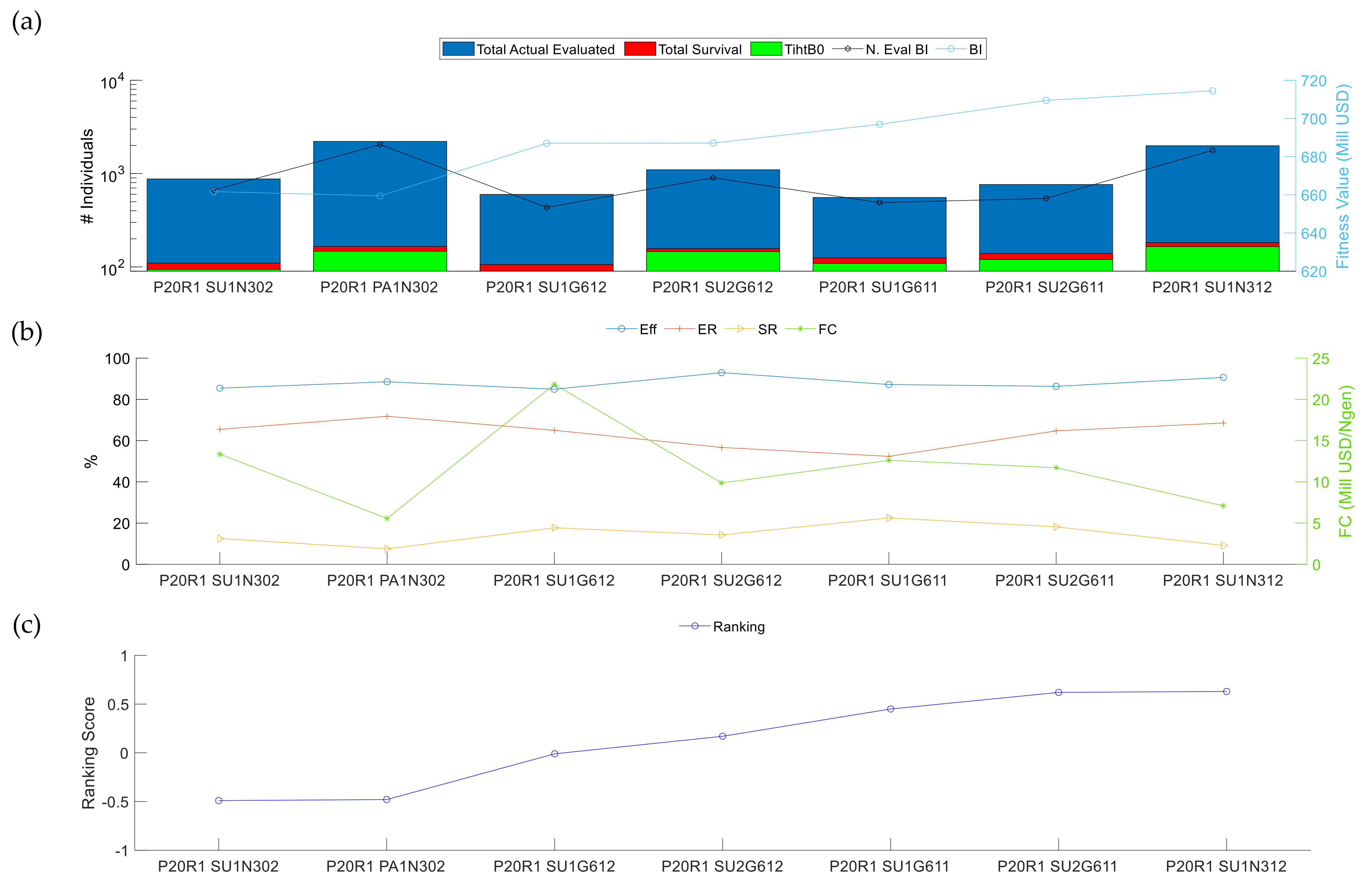
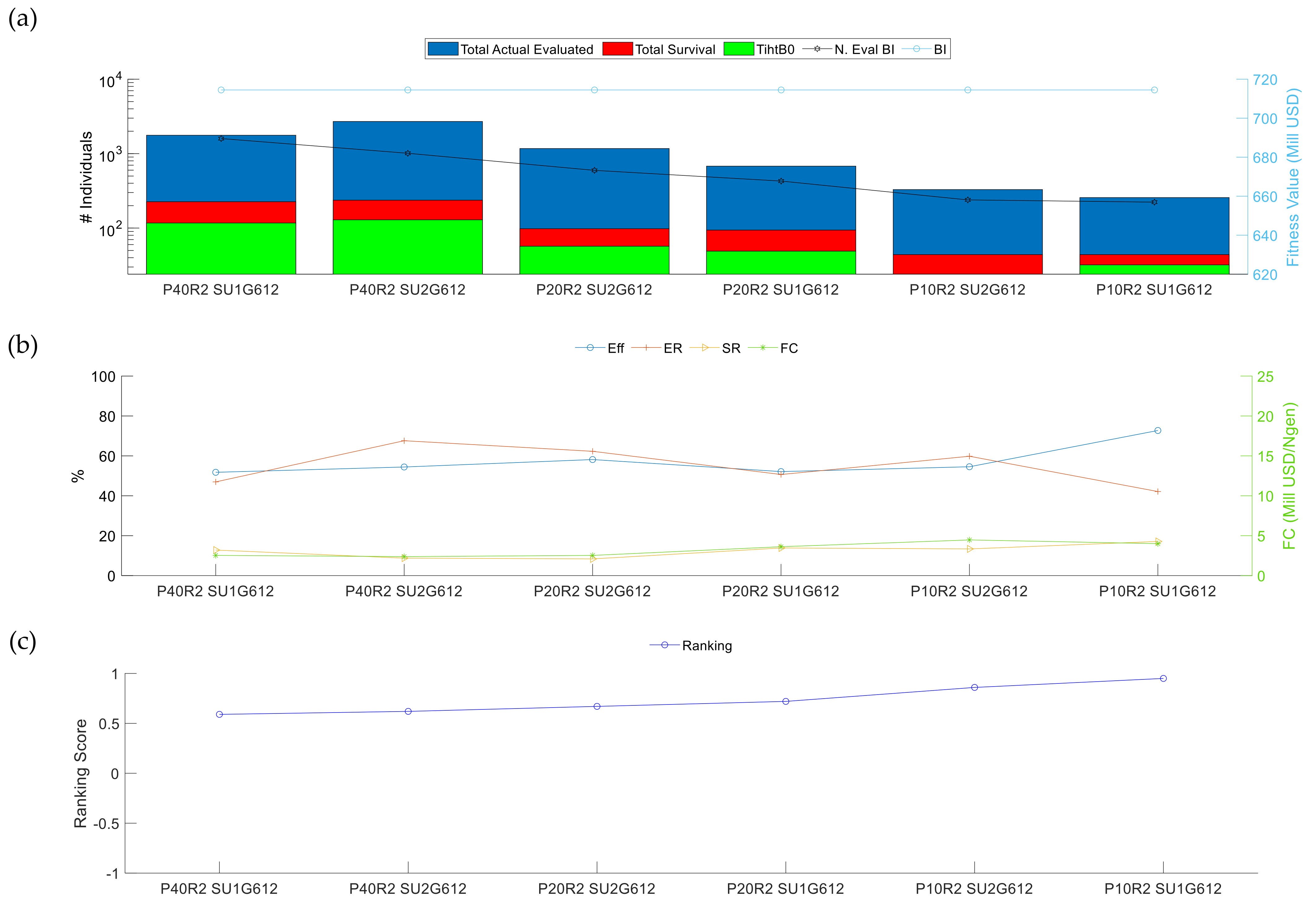
3.2.2. Analysis II: Initial Population Influences

The objective is to define the minimum size of the initial population and the population quality that gives an adequate evolution of the population within a reasonable number of iterations and evaluations.
The evolution performance is highly related to the initial population. For this analysis, a qualitative evaluation of four different initial populations with the same number of individuals was carried out. Thereafter, a sensitivity analysis changing the population size but keeping the initial best individual(s) for larger/extended initial populations sizes was performed. Table 10 indicates how the different populations were generated and their corresponding best individuals.
Populations P20R0, P20R1, and P20R2 were used to evaluate the impact of the initial best individual in the algorithm performance. The results for P20R0 were presented in analysis I, while the results for P20R1 and P20R2 are summarized in Figure 24 and Figure 25, respectively.
The population starting with a low best individual (P20R1) performed poorly when compared with the overall performance of the other two populations. The combination of the structural type of crossover and gradient mutation with a partial mutation rate reached the attraction region, but they did not converge on the best-known value. On the contrary, cases with the same combination of operators but allowing a mutation in both parents and children did not converge on any solution within the attraction region. For this initial condition, the only case able to reach the best-known value was the algorithm that combined the structural type of crossover with a normal mutation in the children and parents (case P20R1SUN312).
An alternative to increasing the probability of obtaining a good initial condition is to apply an extended pre-initialization of the individuals. This extended pre-initialization consists of generating and evaluating a relatively large random population (e.g., 100 individuals) and then selecting the best individuals according to the desired population size. POP 20R2 and POP 20R3 were generated using this extended pre-initialization, and for both cases, the initial fitness value improved significantly with respect to the POP20 R1.
Figure 25 presents the results for POP20R2. The performance of the algorithm for the different cases showed a similar tendency than that observed with POP 20R0, where the combination of a structural crossover with a gradient mutation performed satisfactorily well in comparison with the parametric crossover. For this initial condition, most of the structural crossover cases converged towards the best-known value, except for cases P20R2 SU1G611 and P20R2 SU1N312, which converged on a very similar individual with a fitness value equal to 714.2 mill USD. The corresponding individuals of these two solutions are shown in Table 11. The difference between this solution and the best solution is the type of process separator (two-phase separator vs. three-phase separator). The fitness value for both solutions is very similar, but the uncertainty of the fitness function is very high at the project conceptual stage. Therefore, making a final decision about such similar concepts might require considering additional factors and solving a multiobjective problem instead.
The effect of the population size was analyzed for POPxxR2. Three sizes of populations were selected from the extended pre-initialization results: 40, 20, and 10 best individuals.
In terms of the algorithm performance, the 10-individuals population was good enough to reach the best-known solutions and fulfill the performance indicators for this initial condition satisfactorily (Figure 26). The main advantage was the possibility to reach the best-known values with the fewest evaluations.
A similar behavior was observed when performed a similar analysis using POPxxR3. For this population, the initial best value was below the one for POPxxR2, and the overall p9erformances of all the cases was deficient. Nevertheless, the 10-individual population still performed better than a larger population of 20 individuals in terms of the performance indicators, as shown in Figure 27.
An improvement of the results obtained from POPxxR3 was achieved with the extended pre-initialization when selecting only one best individual and keeping random the rest of the population (POPxxR4). For this initial condition, the population with 10 individuals did not reach the attraction region and ranked last in the cases compared, while populations larger than 20 individuals obtained better outcomes. Thus, limiting the extended pre-initialization to only the best individual improves the performance of the algorithm, but it might require a population of at least 20 individuals.

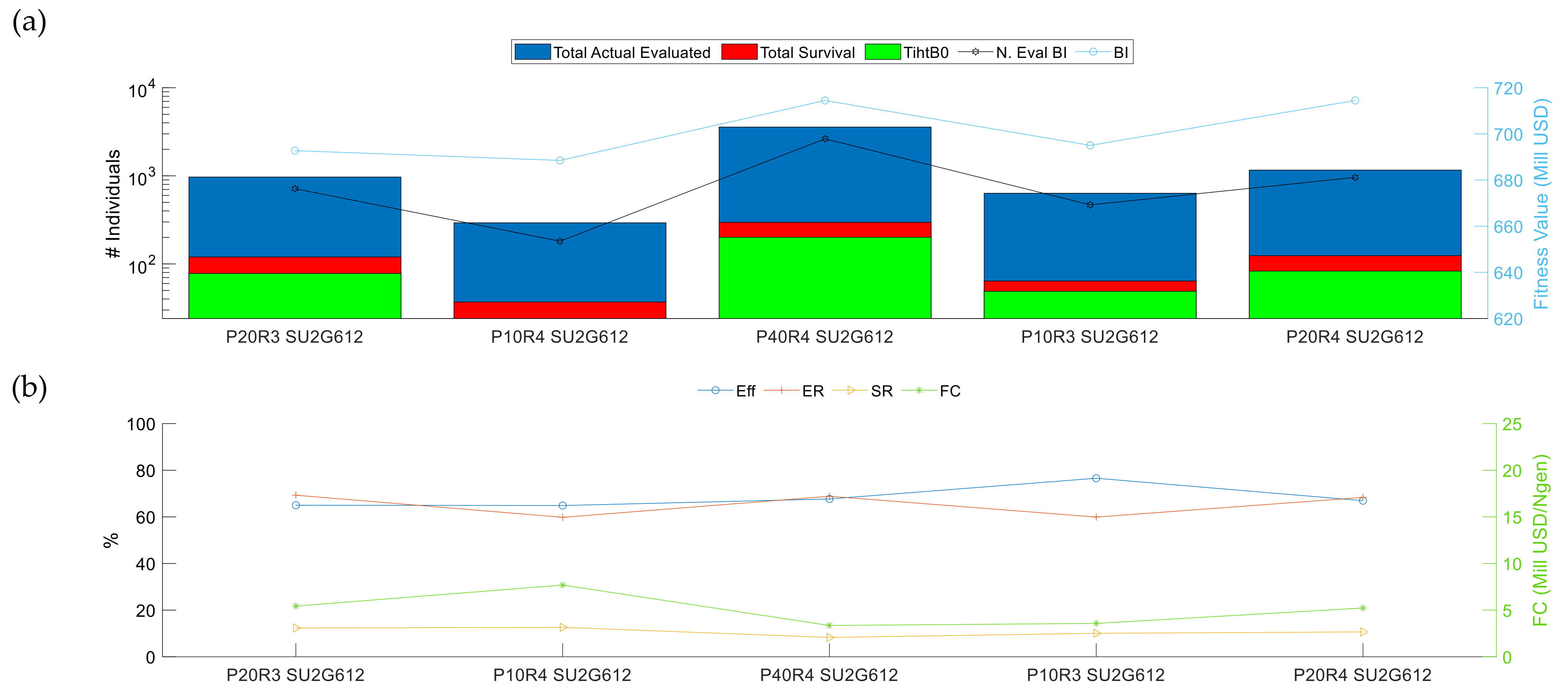
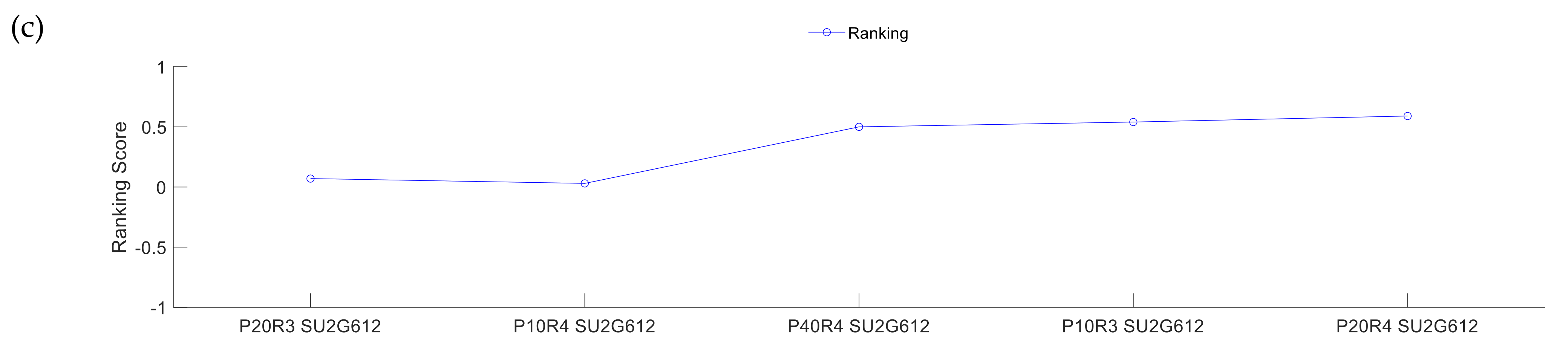
3.2.3. Analysis III: Repeatability of the Results

This study aimed to establish whether the performance observed in analyses I and II are consistent and repeatable. For this analysis, two cases from the previous analyses were repeated five times in order to estimate the effects of the random parameters on the performance of the algorithm. The level of repeatability of the results was measured in terms of the standard deviation of the main measured parameters: total actual evaluations, total survivors, number of generations, TihtB0 (Total individuals higher than best individual in generation 0), N. eval BI (number of evaluations performed before finding the best individual), and BI (Value of the best individual). Table 12 shows the standard deviation and the mean value of the measured variables for the two cases considered, where e ¯ is the average percentage of the standard deviation with respect to the corresponding mean value.
Based on Table 12, the largest deviation of the results corresponds to the counting of the number of the total individuals higher than the best individual in the original generation and to the number of evaluations performed before finding the best individual. The final solution of the problem given by the best individual fitness value presented a relatively consistent behavior with a deviation of around 0.32% of the mean value.

4. Discussion

The optimization problem is centered around maximizing the value of the project using decentralized subsea processing modules considering a given field architecture. The objective function is given by the fitness function represented by the NPV/economic model, which is dependent on the field architecture configuration solution using SGB, as documented in Section 2.5.1. The field architecture configuration solutions are encoded as chromosomes within the EA. They evolve throughout the EA generations to maximize the value of the fitness function, considering relevant problem constraints that are handled by the EA operators, as documented in Section 2.7.3Mutation” and Section 2.7.4.
From the results presented in Section 3, the selection of the crossover operator has a strong influence on the EA performance, but the mutation operator is the key mechanism to achieve the best evolution of the individuals and find a proper solution. When combining a normal mutation with the different alternatives of crossovers, both the parametric arithmetic and the structural uniform showed similar outcomes in terms of the performance indicators. Nevertheless, the performance of the algorithm using a normal mutation was not consistent for all the initial conditions evaluated.
The combination of the structural type of crossover with a gradient mutation showed a significant improvement of the performance, both in terms of the performance indicators and the final solution of the problem. Moreover, by applying this set of variation operators, it was possible to reach, consistently, the attraction region of the solution for the different initial conditions evaluated.
The main advantage of the gradient mutation over the normal mutation is the capacity of controlling and adapting the operator behavior according to the progress of the fitness values. The additional adjustment of the gradient mutation parameters allowed improving the algorithm in terms of convergence precision and speed. The definition of δ is a key factor in the success of this type of mutation. A preliminary sensitivity study of δ and β compared different alternatives to select the appropriate strategy for these parameters. Two alternatives were evaluated: keeping constant values for all generations and generating the parameters randomly at each generation. In this regard, finding a constant value suitable for the fitness changes of all generations proved to be very challenging, and it significantly affected the capacity of the algorithm to evolve towards the near-optimal solution. The second alternative, generating the parameter randomly within a given range for each generation, was more achievable, but it required an adaptive condition for defining the range of the parameters. The range of both parameters must be proportional to the fitness changes, which presents large values for the first generations and tends near zero towards the last generations. The parameter controls given by Equations (26) and (27) were the results of observing and analyzing the different profiles of the fitness changes throughout the generations. During the preliminary analysis, the need for controlling the order of magnitude for the penalization functions and the weighted gradient direction contributions with a different strategy became apparent, as originally defined in [21,43]. The parameter control for this application is dependent on the nature of the crossover operator used before a mutation; therefore, it was decided to define these parameters dynamically or statically, depending on the crossover operator being used. A heuristic crossover, for example, may generate solutions out of the feasible domain, and therefore, it may produce large values of the penalization functions g( C l r x ) during the first generations. Very small values of δ below 0.1 may produce large penalization multipliers and, therefore, large, weighted variations in the mutation, reducing the performance of the gradient contribution. For the rest of the crossover operators listed in this section, this does not occur. Therefore, when using a heuristic crossover operator before a gradient mutation, selecting values of δ between 0.1 and 0.5 is appropriate for this application.
On the other hand, when using the structural uniform crossover, no solutions outside the feasible domain are generated, and therefore, only the penalization function associated with repeated solutions can be activated. For this case, calculating δ based on the inverse average gradient direction of the fitness function for all individuals in the population at each r th generation is proposed, as documented in Equation (26).
Parameter β performs better starting with small values when the gradient is large, increasing proportionally to the generation number to avoid a vanishing gradient contribution when the gradient decreases with the number of generations while approaching an optimal or near-optimal solution. Therefore, the adaptive strategy to control this parameter was proposed, as documented in Equation (27).
The stop criteria were also part of this preliminary study, where different approaches were explored for different population sizes and the maximum number of generations ( N G m a x ).
Another strategy to adjust the gradient mutation operators is through the parent selection method. For this paper, two methods were tested: direct-fitness ranking and direct-fitness-plus-gradient ranking. Both approaches showed similar results according to the performance indicators, although the first approach tended to converge prematurely to a local optimum solution, losing the search energy before reaching the stop criteria. For those cases, the variation operators failed to find new offspring due to the diversity reduction throughout the generations. This behavior was very common for cases with a population size of 10 individuals, and it was seldom registered for a population size of 20 individuals. On the other hand, for cases with parent selection by the direct-fitness-plus-gradient ranking method, a gradient mutation was always capable of reproducing new individuals, even after many generations. Thus, combining both methodologies could be an alternative to consider in future works in order to keep the convergence speed and ensure reaching the stop criteria. A boundary mutation was included as a complementary mutation if required to ensure all solutions were within the feasible domain after the mutation, even though the gradient mutation has penalization functions for unfeasible solutions.
The effect of the mutation rate at different levels of the algorithm seems to have a minor impact on the performance of the EA. The mutation rate applied at the population level did not perform as expected, since the performance was not consistent for the different populations evaluated. The mutation on the children only was more efficient than mutating both the parents and children, probably because the algorithm reached similar solutions while performing fewer evaluations. On the other hand, the mutation rate at the chromosome level appeared to influence the capability of the algorithm to find the fittest individuals. Performing a partial mutation of the chromosome improved the effectiveness of the algorithm when compared with mutating all the genes in the chromosome. However, a further analysis of the precision of the results (Table 12) showed low confidence in the performance indicators related to the effectiveness and the 1/N. eval BI. Therefore, it is difficult to state a conclusion about the improvements observed due to the chromosome mutation rate, and further analyses should be conducted.
The initial condition has a very strong effect on the capability of the EA to find an optimal or near-optimal solution. Applying an extended pre-initialization for selecting the initial population seems to be a fair trade-off between the convergence of the algorithm and the number of evaluations. The extended pre-initialization increases the number of evaluations prior to the first generation, and for complex IPM, this could be a critical factor. However, it does increase the probability of placing good individuals in the initial population and, hence, the probability of reaching an optimum or near-optimum solution without the need for larger population sizes or a larger number of generations. The extended pre-initialization should be used mainly to find the best individual of the initial population and select the remaining individuals randomly from the extended pre-initialized population to promote the initial diversity.
The impact of the population size depends also on the initial condition. For the cases evaluated in this study, a population between 20 to 40 individuals seemed to be good enough to find a solution within the attraction region. Evidently, as the population size increases, both the number of generations and the evaluations per generation also increase. Therefore, the selection of the population size should keep the balance between enabling enough population diversity and keeping the number of evaluations to a minimum. For this work, the stop criteria were constant for all population sizes evaluated; nevertheless, both criteria could be reconsidered for a population of 40 or more individuals.
The total number of evaluations is an important factor to consider for this EA, since it is the most time-consuming section of the whole procedure. The evaluation of each individual is carried out in the IPM software, where the running time depends on the complexity of the model and the optimization variables established within the model. For the purpose of this work, the IPM models did not include any optimization settings, and the average running time per individual was 76.3 s (for a single run). This running time was reduced by using parallel computing that gives the possibility of evaluating several individuals simultaneously. The number of parallel running depends on the size of the cluster and the number of licenses of the IPM software available. For a case with a total evaluation of 819 individuals, 24 generations, and 6 running individuals in parallel, the average running time of the evaluation step in the IPM was about 6.3 h, which represented almost 97% of the total running time of the algorithm.
The best arrangement of the EA was given by combining the structural uniform crossover with a gradient mutation, complemented by a boundary mutation. This EA showed a consistent performance throughout the study, and it was consistently able to find a near-optimal solution within the attraction region when using the extended pre-initialization to generate the initial population.
This work did not consider a sensitivity analysis of the economic parameters or an uncertainty analysis of the results or performances at this stage of the research. The calculations on the repeatability of the results for two of the best settings in Section 3.2.3 were reported to demonstrate the consistency of the solution obtained by the EA.

Future Works

The reservoir model is normally the most computationally time-consuming within the IPM. In this work, a material balance approach was used. Nevertheless, the implementation of a more robust reservoir model might increase significantly the computational time for the overall screening and optimization processes. Different approaches can be implemented to improve the computational time. An interesting option is to combine high-performance parallel simulators and cloud computing, as presented in [44]. The use of “proxy models” is an alternative approach to develop reservoir models with lower computational times. Proxy models intend to represent the simulation model output for a given set of input parameters by solving the mathematical or statistical functions. The authors of [45] proposed an optimization strategy based on a proxy model built from the production potential curves, as explained by [46]. A different alternative was given in [47], where data-driven models were used for real-time optimization during the operation. Although data-driven models are addressed to optimize an operation, it might be possible to use a similar approach for design optimization by generating synthetic data from physical models, as proposed by [48]. Nevertheless, the proxy models approach might require a validation process to assure the accuracy of the model approximation and simplification. For some design stages, a higher accuracy or more flexibility within the search domain in the optimization process may be desirable. Therefore, a hybrid approach might be a good compromise between the accuracy and computational time.
Regarding the EA settings proposed, a similarity among the individuals within the attraction regions might hamper the convergence towards a unique solution. Nevertheless, including an additional variation operator or considering hybrid approaches may contribute to refining the final search in this region.
One of the simplifications introduced to the research work is associated with the economic model, as documented in Section 2.5.1. The selection of the final solution will be limited also by the uncertainty of the fitness function. Therefore, refining the economic model while considering a sensitivity analysis on the model parameters in a real-use case oriented to solve a multi-objective function and including an uncertainty analysis should also be considered for future works.
Explore alternative mechanisms to minimize a premature convergence at the local optimum and/or allow the population to emerge from the local optimum to a different region, such as:
  • Selection mechanisms for population control, considering not only the best individuals but, also, a small number of the worst individuals, as proposed in [49]. Parent selection is performed randomly. Larger population sizes may be required, and therefore, a sensitivity analysis for the population size should be considered.
  • Combination of Direct fitness and gradient rank-based selection methods with the method proposed in [49]. The method documented in [49] can be activated when the gradient vanishes.
  • Multi-start mechanisms for global optimization allow the strategic sampling of the solutions and promote diversification and construction of new solutions for the long-term horizon, as well as balance the diversity and accelerated convergence [50,51,52].
  • Diversity-based adaptive EA [53] not only to prevent a premature convergence to the local optimum but also allow adaptive capabilities for dynamic problems.
The reason to center the focus of this work within the EA domain is supported by their documented applications in similar domain areas, their capabilities to evolve and handle large-scale automated case generation and optimization without the need for explicit analytic models, and the flexibility provided by the different paradigms in terms of data structures that can be used for solution encoding. In addition, there is still a high potential for improvement of the proposed method within the EA domain considering the future works suggested above. However, evaluations and comparisons against alternative relevant metaheuristic optimization methods, such as particle swarm optimization [54,55,56,57] and flower pollination [58,59], should also be considered for future works, as well as hybrid optimization methods.
The other simplification introduced to this research work was to assume the SGB configuration to be fixed during the field life, neglecting the performance variations of the processing equipment due to the production profile changes over time. Therefore, it will be relevant to include a time variable within the EA encoding to explore the evolution of the decentralized processing system through the lifetime of the field.

5. Conclusions

Traditional field development processes involve multiple disciplines and technical domains working in silos with their own engineering software and tools. The concept development processes involving scenario screening are normally manual and time-consuming. Therefore, the possible options are normally reduced to a limited number of discrete solutions or sensitivity cases that do not necessary lead to an optimal field architecture.
This work presented a methodology that combined evolutionary algorithms (EA) and an integrated production modeling (IPM) approach to automate case generation, field architecture scenario screening, and optimization when using decentralized subsea processing modules during field development. The objective of the methodology was to outline the best arrangement of the decentralized processing systems for a given field architecture according to an optimization criterion.
The EA enables a systematic screening process that allows exploring the entire domain, ranking the alternatives, and finding a near-optimal solution in a consistent manner. The exploration mechanism provided by the EA makes possible searching within the domain without evaluating every scenario. Thus, the EA is responsible for guiding the search and making evolve a set of solutions to satisfy the optimization problem. The IPM, on the other hand, contains the logistics for evaluating the fitness function, decoding the scenarios defined by the EA, and reconfiguring the field architecture accordingly. This decoding procedure utilizes a superstructure representation of the problem that allows the generation and evaluation of the different scenarios. The EA and the IPM are connected by the “Evaluation” step within the EA (Section 2.7.6) implemented for the experimental settings by connecting the Petroleum Expert Software with MATLAB using the OpenServer utility. Such an interface allows carrying out the scenario screening and optimization using decentralized subsea processing systems in an automated manner.
This paper explored the capability of the EA to support automated scenario generation, screening, and optimization. Thus, this study focused on the evaluation of various genetic operators and evolution strategies to compare their performances. The scope of this analysis included the comparisons and evaluations of the variation operators (crossover and mutation), impact of the initial population, and repeatability of the results.
The study was performed using a synthetic business case where the screening matrix considered the selection of six (6) different processes to place at six (6) possible locations within a fixed field architecture. The total search domain for the study case was 1.5 × 10⁹ possible scenarios. The problem formulation consisted of designing the decentralized processing system that satisfied an optimization criterion. For this work, the optimization problem was addressed to maximize the economic value of the architecture by calculating a simplified model of the additional NPV. The final solution of the methodology provided information on the number of decentralized subsea processing systems required (subsea gate box: SGB), location of the individual SGB, and their corresponding internal configurations (numbers and types of process units).
For the business case evaluated, the best-known cost-effective solution is to implement the decentralized processing system locating a SGB with gas–liquid separator and liquid boosting at the two main commingling points (manifold field B and the manifold that tied field B back to field A) and one three-phase separator at well L4 at field B. The fitness value for such architecture reached a project value of 714.5 mill USD. The solution was found after 28 interactions and 1162 simulations of the IPM, with an approximate total running time of 6.54 h.
Regarding the variation operators evaluated within the EA, the sensitivity analysis of the different parameters and types of operators considered showed that the best performance of the EA was provided by a combination of the structural uniform crossover with a mutation along the weighted gradient direction and a complementary boundary mutation (corresponding to cases P20R0 SUxG6xx and P20R0 SUxG6xx). Such EA settings were able to find the best-known solution (BKS) or solutions within one standard deviation of the BKS in a consistent manner. The parameters associated with the chromosome mutation rate, population mutation rate, and parent selection method did not show a significant impact on the capacity of those cases to reach the best-known solution. These variables mainly affected the algorithm in terms of the convergence speed and effectiveness.
The poorest performance was observed when combining a structural segmented crossover with the normal plus boundary mutation (case P20R0 SS1N202) and combining a parametric arithmetic crossover with a gradient plus boundary mutation (case P20R0 PA1G611). In general, the cases combining a normal plus boundary mutation with a crossover operator, such as the parametric-heuristic, parametric average, structural segmented, and random structural uniform, did not find any solution within one standard deviation of the best-known value. Likewise, cases combining the gradient plus boundary mutation with the parametric-heuristic and parametric averages also failed to reach this attraction region.
It was observed that, while the crossover operator has a strong influence on the EA performance, the mutation operator was the key mechanism to achieve the best evolution of the individual and finding a near-optimal solution. In this context, the gradient mutation operator has the capacity to control and adapt the operator behavior according to the progress of the fitness value. The adaptive capabilities of δ and β are crucial in the success of weighted gradient direction.
The initial condition has a very strong effect on the capability of the EA to find the near optimal solution. A reasonable compromise between the number of evaluations and the convergence speed of the algorithm is to apply a pre-initialization for selecting the initial population. This pre-initialization increases the number of evaluations prior to the first generation to increase the possibility of placing a relatively good individual in the initial population.
The size of the population is a critical parameter that might define the feasibility of the algorithm. For the cases evaluated in this study, a population between 20 and 40 individuals was good enough to find the best-known value. The case with a population of 40 individuals did not improve the algorithm performance, and it required a significantly larger number of evaluations.
The EA algorithm developed at this stage does not guarantee a global optimal solution, such as a meta-heuristic optimization, but it is the starting point to develop and automate a scenario screening tool and, eventually, contribute a building block for the future asset development digital twin.
Although the main optimization problem for this work is based on the design of the subsea gate box concept (decentralized subsea processing) [1,2], the methodology could be adapted to optimize other variables within the field architecture, including artificial lift methods, well routing, delivery/export routing, etc. This adaptation, however, might require a different encoding of the solution, testing, and verification of the relevant genetic operators and evolution strategies for the additional variables.
Future works will focus on the further development of this algorithm to improve global search and optimization capabilities, refine the economic model, include an uncertainty analysis, and consider SGB configuration changes that may be needed throughout the field life. A comparative analysis and/or hybrid solutions with alternative, relevant metaheuristic optimization methods outside the EA domain are also being considered for future works.

Author Contributions

Conceptualization, M.J.C.D.A. and E.A.; methodology, M.J.C.D.A. and E.A.; software, M.J.C.D.A. and A.M.d.S.; validation, M.J.C.D.A., A.M.d.S., and E.A.; formal analysis, M.J.C.D.A. and E.A.; investigation, M.J.C.D.A. and E.A.; resources, M.J.C.D.A., A.M.d.S., and E.A.; data curation, M.J.C.D.A.; writing—original draft preparation, M.J.C.D.A. and E.A.; writing—review and editing, M.J.C.D.A. and E.A.; visualization, M.J.C.D.A.; supervision, E.A. All authors have read and agreed to the published version of the manuscript.

Funding

This research was funded by the Norwegian Centre for Research-based Innovation on Subsea Production and Processing (SUBPRO), grant number 237893.

Institutional Review Board Statement

Not applicable.

Informed Consent Statement

Not applicable.

Data Availability Statement

Data generated from the integrated production model during the project from the multiple sensitivity cases, as well as the Subsea Gate Box Configuration Matrix used for the Synthetic Field, can be made available on request. The computational code is at research stage TRL0-1 based on the API-17 N TRL ladder; no software product development process has been applied yet. The software code was only generated and used to test the methodology proposed in this work. A comprehensive documentation of the algorithm details considering all the operators that were tested, as well as the evaluation KPIs used for the comparative analysis, are thoroughly described in the paper. Therefore, the available information is considered sufficient to generate the relevant software code to reproduce these results.

Acknowledgments

The authors greatly acknowledge the financial support by the Research Council of Norway, as well as the industrial partners involved in the SUBPRO consortium. Furthermore, the NTNU authors would like to thank Aker BP ASA for the collaboration, technical support, and guidance.

Conflicts of Interest

The authors declare no conflict of interest.

References

  1. Diaz, M.J.C.; Stanko, M.; Sangesland, S. Exploring New Concepts in Subsea Field Architecture. In Proceedings of the Offshore Technology Conference, Houston, TX, USA, 30 April–3 May 2018; p. 14. [Google Scholar]
  2. Diaz, M.J.C.; Sangesland, S.; Stanko, M. The subsea gate box: And alternative subsea filed architecture. First SPE Nor. Mag. 2018, 2, 38. Available online: http://oslo.spe.org/thefirst (accessed on 18 January 2021).
  3. Diaz, M.; Sangesland, S.; Stanko, M. Enabling Flexible Subsea Architecture for Production Field with Large Heterogeneity among Wells; Internal Report; Norwegian University of Science and Technology: Trondheim, Norway, 2019; Unpublished. [Google Scholar]
  4. Irmann-Jacobsen, T.B.; Headridge, B. Ultimate Gas Recovery by Use of Full Field Simulations in Concept Selection Phase. In Proceedings of the Offshore Technology Conference-Asia, Kuala Lumpur, Malaysia, 25–28 March 2014; p. 11. [Google Scholar]
  5. Dianita, S.; Gandi, R.S. Full Field Integrated Modelling throughout Life-Cycle Phases of Field Development: A Subsea Processing Case Study. In Proceedings of theSPE/IATMI Asia Pacific Oil & Gas Conference and Exhibition, Nusa Dua, Bali, Indonesia, 20–22 October 2015; p. 15. [Google Scholar]
  6. Sauve, R.; Lindvig, T.; Stenhaug, M.; Holyfield, S. Integrated Field Development: Process and Productivity. In Proceedings of the Offshore Technology Conference, Houston, TX, USA, 6–9 May 2019; p. 19. [Google Scholar]
  7. Narayanan, K.; Cullick, A.S.; Matthew, B. Better Field Development Decisions from Multi-Scenario, Interdependent Reservoir, Well, and Facility Simulations. In Proceedings of the SPE Reservoir Simulation Symposium, Houston, TX, USA, 3–5 February 2003; p. 11. [Google Scholar]
  8. Smyth, J.; Rusin, P.; Garcia, J.J.; Cullick, S. Rapid Optimization of Development Scenarios for Multiple Exploration Prospects Using Integrated Asset Modeling. In Proceedings of the SPE Latin American and Caribbean Petroleum Engineering Conference, Lima, Peru, 1–3 December 2010; p. 21. [Google Scholar]
  9. Bouamra, R.; Vielliard, C.; Spilling, K.E.; Nilsen, F.P. Integrated Production Management Solution for Maximized Flow Assurance and Reservoir Recovery. In Proceedings of the OTC Brasil, Offshore Technology Conference, Rio de Janeiro, Brazil, 24–26 October 2017; p. 9. [Google Scholar]
  10. Saputelli, L.A.; Lujan, L.; Garibaldi, L.; Smyth, J.; Ungredda, A.; Rodriguez, J.; Cullick, S. How Integrated Field Studies Help Asset Teams Make Optimal Field Development Decisions. In Proceedings of the SPE Western Regional and Pacific Section AAPG Joint Meeting, Bakersfield, CA, USA, 29 March–4 April 2008; p. 16. [Google Scholar]
  11. Ogunyomi, B.A.; Jablonowski, C.J.; Lake, L.W. Field Development Optimization under Uncertainty: Screening-Models for Decision Making. In Proceedings of the SPE Annual Technical Conference and Exhibition, Denver, CO, USA, 30 October–2 November 2011; p. 11. [Google Scholar]
  12. Mikhin, A.; Salavatullin, K.; Kamartdinov, M. Main Aspects of the Integrated Asset Modeling and Gas Field Development Optimization under Surface Facilities Constraints. In Proceedings of the SPE Russian Petroleum Technology Conference, Moscow, Russia, 15–17 October 2018; p. 13. [Google Scholar]
  13. Rosa, V.R.; Camponogara, E.; Ferreira Filho, V.J.M. Design optimization of oilfield subsea infrastructures with manifold placement and pipeline layout. Comput. Chem. Eng. 2018, 108, 163–178. [Google Scholar] [CrossRef]
  14. Wang, Y.; Estefen, S.F.; Lourenço, M.I.; Hong, C. Optimal design and scheduling for offshore oil-field development. Comput. Chem. Eng. 2019, 123, 300–316. [Google Scholar] [CrossRef]
  15. Teixeira, A.F.; de Campos, M.; Barreto, F.P.; Stender, A.S.; Arraes, F.F.; Rosa, V.R. Model Based Production Optimization Applied to Offshore Fields. In Proceedings of the OTC Brasil, Offshore Technology Conference, Rio de Janeiro, Brazil, 29–31 October 2013; p. 11. [Google Scholar]
  16. Lin, P.; Bao, X.; Shu, Z.; Wang, X.; Liu, J. Test case generation based on adaptive genetic algorithm. In Proceedings of the 2012 International Conference on Quality, Reliability, Risk, Maintenance, and Safety Engineering, Chengdu, China, 15–18 June 2012. [Google Scholar]
  17. Khan, R.; Amjad, M. Automatic test case generation for unit software testing using genetic algorithm and mutation analysis. In Proceedings of the 2015 IEEE UP Section Conference on Electrical Computer and Electronics (UPCON), Allahabad, India, 4–6 December 2015. [Google Scholar]
  18. Mateen, A.; Nazir, M.; Afsar, S. Optimization of Test Case Generation using Genetic Algorithm (GA). Int. J. Comput. Appl. 2016, 151, 6–14. [Google Scholar] [CrossRef]
  19. Khan, R.; Amjad, M.; Srivastava, A.K. Optimization of Automatic Generated Test Cases for Path Testing Using Genetic Algorithm. In Proceedings of the 2016 Second International Conference on Computational Intelligence & Communication Technology (CICT), Ghaziabad, India, 12–13 February 2016. [Google Scholar]
  20. Khan, R.; Amjad, M.; Srivastava, A.K. Generation of automatic test cases with mutation analysis and hybrid genetic algorithm. In Proceedings of the 2017 3rd International Conference on Computational Intelligence & Communication Technology (CICT), Ghaziabad, India, 9–10 February 2017. [Google Scholar]
  21. Altamiranda, E.; Calderón, R.; Morles, E. An Evolutionary Algorithm for Linear System Identification. In Proceedings of the 6th WSEAS International Conference on Signal Processing, Robotics and Automation, Corfu Island, Greece, 16–17 February 2007. [Google Scholar]
  22. Radatz, H.; Schröder, M.; Becker, C.; Bramsiepe, C.; Schembecker, G. Selection of equipment modules for a flexible modular production plant by a multi-objective evolutionary algorithm. Comput. Chem. Eng. 2019, 123, 196–221. [Google Scholar] [CrossRef]
  23. Nagaiah, N.R.; Geiger, C.D. Application of evolutionary algorithms to optimize cooling channels. Int. J. Simul. Multidiscip. Des. Optim. 2019, 10, A4. [Google Scholar] [CrossRef] [Green Version]
  24. Healey, M.; Duff, S.; James, J. Optimization of a Subsea Design using an Evolutionary Algorithm. In Proceedings of the BHR 19th International Conference on Multiphase Production Technology, Cannes, France, 5–7 June 2019; p. 12. [Google Scholar]
  25. Castiñeira, P.P.; Baioco, J.S.; Couto, P.; Jacob, B.P. Optimal Positioning of Submarine Manifolds through Genetic Algorithms. In Proceedings of the 26th International Ocean and Polar Engineering Conference, Rhodes, Greece, 26 June–1 July 2016; International Society of Offshore and Polar Engineers: Rhodes, Greece; p. 5. [Google Scholar]
  26. Salam, D.D.; Gunardi, I.; Yasutra, A. Production Optimization Strategy Using Hybrid Genetic Algorithm. In Proceedings of the Abu Dhabi International Petroleum Exhibition and Conference, Abu Dhabi, UAE, 9–12 November 2015; p. 14. [Google Scholar]
  27. Motie, M.; Moein, P.; Moghadasi, R.; Hadipour, A. Separator Pressure Optimisation and Cost Evaluation of a Multistage Production Unit Using Genetic Algorithm. In Proceedings of the International Petroleum Technology Conference, Beijing, China, 26–28 March 2019; p. 14. [Google Scholar]
  28. Sambo, C.H.; Hematpour, H.; Danaei, S.; Herman, M.; Ghosh, D.P.; Abass, A.; Elraies, K.A. An Integrated Reservoir Modelling and Evolutionary Algorithm for Optimizing Field Development in a Mature Fractured Reservoir. In Proceedings of the Abu Dhabi International Petroleum Exhibition & Conference, Abu Dhabi, UAE, 7–10 November 2016; p. 10. [Google Scholar]
  29. Sayyafzadeh, M. A Self-Adaptive Surrogate-Assisted Evolutionary Algorithm for Well Placement Optimization Problems. In Proceedings of the SPE/IATMI Asia Pacific Oil & Gas Conference and Exhibition, Nusa Dua, Bali, Indonesia, 20–22 October 2015; p. 16. [Google Scholar]
  30. Henao, C.A. A Superstructure Modeling Framework for Process Synthesis Using Surrogate Models. In Chemical Engineering; University of Wisconsin-Madison: Madison, WI, USA, 2012; p. 210. [Google Scholar]
  31. Quaglia, A. An Integrated Business and Engineering Framework for Synthesis and Design of Processing Networks; Department of Chemical and Biochemical Engineering, Technical University of Denmark: Kongens Lyngby, Denmark, 2013; p. 240. [Google Scholar]
  32. Bertran, M.O.; Frauzem, R.; Zhang, L.; Gani, R. A Generic Methodology for Superstructure Optimization of Different Processing Networks. In Computer Aided Chemical Engineering; Kravanja, Z., Bogataj, M., Eds.; Elsevier: Amsterdam, The Netherlands, 2016; pp. 685–690. [Google Scholar]
  33. Khor, C.S.; Elkamel, A. Superstructure Optimization for Oil Refinery Design. Pet. Sci. Technol. 2010, 28, 1457–1465. [Google Scholar] [CrossRef]
  34. Krogstad, D. Superstructure Optimization of a Subsea Separation System; Department of Chemical Engineering, Norwegian University of Science and Technology: Trondheim, Norway, 2017. [Google Scholar]
  35. Rahmawati, S.D.; Whitson, C.H.; Foss, B.; Kuntadi, A. Integrated field operation and optimization. J. Pet. Sci. Eng. 2012, 81, 161–170. [Google Scholar] [CrossRef]
  36. ISO. Petroleum and natural gas industrues. Life-cycle costing. In Guidance on Application of Methodology and Calculations Methods; ISO: Geneva, Switzerland, 2001; p. 36. [Google Scholar]
  37. QUE$TOR 2019 Q3’s Help File; HIS Markit Inc.: Englewood, CO, USA, 2019.
  38. Aguilar, J.; Rivas, F. Computación Evolutiva. In Introducción a las Técnicas de Computación Inteligente; Universidad de Los Andes: Mérida, Venezuela, 2001. [Google Scholar]
  39. Yu, X.; Gen, M. Introduction to Evolutionary Algorithms; Decision Engineering; Springer: London, UK, 2010. [Google Scholar]
  40. Ackora-Prah, J.; Gyamerah, S.A.; Andam, P.S. A heuristic crossover for portfolio selection. Appl. Math. Sci. 2014, 8, 3215–3227. [Google Scholar] [CrossRef]
  41. Umbarkar, A.J.; Sheth, P.D. Crossover operators in genetic algorithms: A review. ICTACT J. Soft Comput. 2015, 6, 1083–1092. [Google Scholar]
  42. Hassanat, A.; Almohammadi, K.; Alkafaween, E.; Abunawas, E.; Hammouri, A.; Prasath, V.B.S. Choosing Mutation and Crossover Ratios for Genetic Algorithms—A Review with a New Dynamic Approach. Information 2019, 10, 390. [Google Scholar] [CrossRef] [Green Version]
  43. Jiafu, T.; Dingwei, W. A new genetic algorithm for nonlinear programming problems. In Proceedings of the 36th IEEE Conference on Decision and Control: San Diego, CA, USA, 12 December 1997. [Google Scholar]
  44. Tanaka, S.; Wang, Z.; Dehghani, K.; He, J.; Velusamy, B.; Wen, X.H. Large Scale Field Development Optimization Using High Performance Parallel Simulation and Cloud Computing Technology. In Proceedings of the SPE Annual Technical Conference and Exhibition, Dallas, TX, USA, 24–26 September 2018; p. 22. [Google Scholar]
  45. Gonzalez, D. Methodologies to Determine Cost-Effective Development Strategies for Offshore Fields during Early-Phase Studies Using Proxy Models and Optimization; Department of Geoscience and Petroleum, Faculty of Engineering, Norwegian University of Science and Technology: Trondheim, Norway, 2020. [Google Scholar]
  46. Stanko, M. Observations on and use of curves of current dimensionless potential versus recovery factor calculated from models of hydrocarbon production systems. J. Pet. Sci. Eng. 2021, 196, 108014. [Google Scholar] [CrossRef]
  47. Gobel, D.; Briers, J.; Chin, Y.M. Architecture and Implementation of an Optimization Decision Support System. In Proceedings of the International Petroleum Technology Conference, Beijing, China, 26–28 March 2013; p. 18. [Google Scholar]
  48. Cadei, L.; Rossi, G.; Montini, M.; Fier, P.; Milana, D.; Corneo, A.; Sophia, G. Machine Learning Advanced Algorithm to Enhance Production Optimization: An ANN Proxy Modelling Approach. In Proceedings of the International Petroleum Technology Conference, Dhahran, Kingdom of Saudi Arabia, 13–15 January 2020; p. 14. [Google Scholar]
  49. Jamróz, D.; Niedoba, T.; Pięta, P.; Surowiak, A. The Use of Neural Networks in Combination with Evolutionary Algorithms to Optimise the Copper Flotation Enrichment Process. Appl. Sci. 2020, 10, 3119. [Google Scholar] [CrossRef]
  50. Hickernell, F.J.; Yuan, Y. A simple multistart algorithm for global optimization. OR Trans. 1997, 1, 1–12. [Google Scholar]
  51. Martí, R.; Resende, M.G.C.; Ribeiro, C.C. Multi-start methods for combinatorial optimization. Eur. J. Oper. Res. 2013, 226, 1–8. [Google Scholar] [CrossRef]
  52. Tu, W.; Mayne, R. Studies of multi-start clustering for global optimization. Int. J. Numer. Methods Eng. 2002, 53, 2239–2252. [Google Scholar] [CrossRef]
  53. Gouvea, M.; Ribeiro, A. Diversity-Based Adaptive Evolutionary Algorithms. In New Achievements in Evolutionary Computation; Korosec, P., Ed.; Intech Slovenia: Ljubljana, Slovenia, 2010; p. 318. ISBN 978-953-307-053-7. [Google Scholar]
  54. Panahli, C.; Kleppe, J.; Bellout, M. Implementation of Particle Swarm Optimization Algorithm within FieldOpt Optimization Framework. Master’s Thesis, NTNU, Trondheim, Norway, 2017. Available online: http://hdl.handle.net/11250/2453090 (accessed on 10 January 2021).
  55. Onwunalu, J.; Durlofsky, L. Optimization of Field Development Using Particle Swarm Optimization and New Well Pattern Descriptions. Ph.D. Thesis, Stanford University, Stanford, CA, USA, 2010. Available online: http://purl.stanford.edu/tx862dq9251 (accessed on 10 January 2021).
  56. Windisch, A.; Wappler, S.; Wegner, J. Applying Particle Swarm Optimization to Software Testing. In Proceedings of the 9th Annual Conference on Genetic and Evolutionary Computation, London, UK, 7–11 July 2007. [Google Scholar]
  57. Adibifard, M.; Bashiri, G.; Roayaei, E.; Emad, M.A. Using Particle Swarm Optimization (PSO) Algorithm in Nonlinear Regression Well Test Analysis and Its Comparison with Levenberg-Marquardt Algorithm. Int. J. Appl. Metaheuristic Comput. 2016, 7, 1–23. [Google Scholar] [CrossRef]
  58. Suwannarongsri, S. Optimal Sizing of Hybrid Renewable Energy System via Flower Pollination Algorithm. WSEAS Trans. Environ. Dev. 2019, 15, 240–249. [Google Scholar]
  59. Yang, X.S. Flower Pollination Algorithm for Global Optimization. In Unconventional Computation and Natural Computation; Durand-Lose, J., Jonoska, N., Eds.; Springer: Berlin/Heidelberg, Germany, 2012; Volume 7445. [Google Scholar] [CrossRef] [Green Version]
Figure 1. Subsea gate box concept [3].
Processes 09 00184 g001
Figure 2. Possible process modules within a subsea gate box (SGB).
Processes 09 00184 g002
Figure 3. Flow diagram of the case generation and scenario screening methodology. EA: evolutionary algorithms and IPM: integrated production modeling.
Processes 09 00184 g003
Figure 4. Superstructure example. (A) Original field layout from the input file, (B) superstructure file, and (C) subsea gate box internal superstructure.
Processes 09 00184 g004aProcesses 09 00184 g004b
Figure 5. Superstructure identification system.
Processes 09 00184 g005
Figure 6. Integrated production model diagram.
Processes 09 00184 g006
Figure 7. Sketch of the subsea gate box assembly.
Processes 09 00184 g007
Figure 8. Example of a configuration matrix.
Processes 09 00184 g008
Figure 9. Case definition constraints.
Processes 09 00184 g009
Figure 10. EA Chromosome configuration for the SGB field configuration cases.
Processes 09 00184 g010
Figure 11. Segmented crossover with p = 1.
Processes 09 00184 g011
Figure 12. Example of the structural uniform crossover, mirroring ¬ O l r x for the second child
Processes 09 00184 g012
Figure 13. Proposed evolutionary algorithm flow diagram.
Processes 09 00184 g013
Figure 14. Oil field business case.
Processes 09 00184 g014
Figure 15. Business Case Solution.
Processes 09 00184 g015
Figure 16. Selected scenario.
Processes 09 00184 g016
Figure 17. Example of the evolution of the fitness function.
Processes 09 00184 g017
Figure 18. Comparison of the initial generation (a) vs. the last generation (b).
Processes 09 00184 g018
Figure 19. Example of the case analysis identification tag.
Processes 09 00184 g019
Figure 20. Summary of the performance indicators for analysis I, Section 1. (a) shows variables of KPI 3,4 and 5 in bar chart, KPI 1 and variable of KPI 7 in line chart, (b) shows KPI 3,4,5 and 6 in line chart, (c) shows the ranking score based on Table 8.
Processes 09 00184 g020
Figure 21. Summary of the performance indicators for analysis I, Section 2. (a) shows variables of KPI 3,4 and 5 in bar chart, KPI 1 and variable of KPI 7 in line chart, (b) shows KPI 3,4,5 and 6 in line chart, (c) shows the ranking score based on Table 8.
Processes 09 00184 g021
Figure 22. Summary of the performance indicators for analysis I, Section 3. (a) shows variables of KPI 3,4 and 5 in bar chart, KPI 1 and variable of KPI 7 in line chart, (b) shows KPI 3,4,5 and 6 in line chart, (c) shows the ranking score based on Table 8.
Processes 09 00184 g022
Figure 23. Comparison of the most relevant cases of analysis I.
Processes 09 00184 g023
Figure 24. Summary of the performance indicators for POP20 R1. (a) shows variables of KPI 3,4 and 5 in bar chart, KPI 1 and variable of KPI 7 in line chart, (b) shows KPI 3,4,5 and 6 in line chart, (c) shows the ranking score based on Table 8.
Processes 09 00184 g024
Figure 25. Summary of the performance indicators for POP20 R2. (a) shows variables of KPI 3,4 and 5 in bar chart, KPI 1 and variable of KPI 7 in line chart, (b) shows KPI 3,4,5 and 6 in line chart, (c) shows the ranking score based on Table 8.
Processes 09 00184 g025
Figure 26. Summary of the performance indicators for the different populations sizes (POP xxR2). (a) shows variables of KPI 3,4 and 5 in bar chart, KPI 1 and variable of KPI 7 in line chart, (b) shows KPI 3,4,5 and 6 in line chart, (c) shows the ranking score based on Table 8.
Processes 09 00184 g026
Figure 27. Summary of the performance indicators comparing POP xxR3 vs. POP xxR4. (a) shows variables of KPI 3,4 and 5 in bar chart, KPI 1 and variable of KPI 7 in line chart, (b) shows KPI 3,4,5 and 6 in line chart, (c) shows the ranking score based on Table 8.
Processes 09 00184 g027aProcesses 09 00184 g027b
Table 1. Main cost elements within an economic evaluation method established by the standard ISO 15663-2:2001(E). Adapted from [36].
CAPEX“Cover the relevant initial investment outlay Io, from discovery through appraisal, engineering, construction, and commissioning including modifications until normal operations are achieved.”
OPEX“Cover the relevant costs over the lifetime of operating and maintaining the asset.”
Revenue impact“Cover the relevant impact on the revenue stream from failures leading to production shutdowns, planned shutdowns, and penalties.”
Disposal/decommissioning“Cover relevant costs of abandonment of the asset, if there will be a cost difference between alternatives evaluated.”
Table 2. Fitness function spreadsheet to calculate Equation (1). SGB: subsea gate box.
Date (dd/mm/yyyy)Time Step in Resolve Simulations. Starting Time = Production Startup
# daysCumulative number of days at each time step. This corresponds to the time step into the future (t) in Equation (1). Starting time = two years prior to production startup.
Base Case Qo (MSm3)Cumulative Oil/Gas production at each time step for the base case scenario. The base case scenario is the original field without subsea processing or subsea gate boxes.
Base Case Qg (MSm3)
Current Case Qo (MSm3)Cumulative Oil/Gas production at each time step for the evaluated case. The evaluated case is one case among all possible SGB configurations.
Current Case Qg (MSm3)
Extra Qo (m3)Extra Oil/Gas production due to the modifications implemented in the evaluated case. This is the difference between the cumulative production of the evaluated case and the base case.
Extra Qg (Sm3)
Energy (MWh)Power consumption of pumps and compressors of the different SGB.
Extra Qo (USD)Incomes of the extra Oil/Gas sells. Oil price (50 USD).
Extra Qg (USD)
Energy (USD)Expenditure for the energy consumption of the pumps and compressors of the different SGB (32 USD/MWH).
CAPEX (USD)Capital expenditure according to the items in Table 3. The CAPEX is uniformly distributed during the two years prior to the first oil.
OPEX (USD)Operational expenditure according to the items in Table 4.
Incomes (USD)Sum of the incomes for the extra oil and gas.
Costs (USD)Sum of the expenditure associated with the SGB.
S t (USD)Net balance at the end of the time step.
FF (USD)Equation (1) (discount rate = 10%).
Table 3. Simplified CAPEX structure.
LevelWBS IDProject WBS Item Description
Level 00X Project Development
Level 11Facilities
Level 2101Subsea
Level 310101SGB
Level 41010101Equipment
Level 5101010101Multiphase Boosting
Level 5101010102Oil Boosting
Level 5101010103Water Boosting
Level 5101010104Gas Boosting
Level 5101010105Gas–Liquid Separation
Level 5101010106Oil–Water Separation
Level 5101010107Heater
Level 5101010108Interconnection Module
Level 610101010801Structure
Level 610101010802Piles
Level 610101010803Manifold
Level 610101010804Subsea Distribution Unit
Level 610101010805Subsea Control Unit
Level 610101010806Internal Connectors
Level 5101010109Equipment Freight
Level 310102Subsea Network
Level 41010201Equipment
Level 5101020101Umbilical Connector Type 1
Level 5101020102Umbilical Connector Type 2
Level 5101020103Subsea Distribution Unit *
Level 5101020104Equipment Freight
Level 41010202Material
Level 5101020207PLET (Pipeline End Termination)
Level 5101020208Flowline
Level 5101020209Power cable Static-Umbilical
Level 5101020210Power cable Dynamic Umbilical
Level 5101020211Riser
Level 5101020212Material Freight
Level 2102Topside
Level 310201Power Generation
Level 310202Topside VSds (Variable Speed Drives) *
* These items were not required for the business case used for this paper. WBS: Work Breakdown Structure.
Table 4. Items considerer for the OPEX.
DSV For Inspection (days)0
MSV For Repair (days)f (Number of equipment)
Spares Costs (% CAPEX)1%
Reconditioning Cost (%Equipment without Freight)2%
Insurance OPEX (%CAPEX)0.5%
DSV: Diving Support Vessel. MSV: Multipurpose support/supply vessel.
Table 5. Cost structure of a subsea multiphase pump.
ItemQuantityUnit Price
Pump station steel frameF1(Tkw)tefixUSD
Pumps and motors1undF2(Tkw)USD
Subsea control module 1undfixUSD
Subsea step-down transformer0undF3(Tkw)USD
Subsea variable speed drive0undF4(Tkw)USD
Multiphase pumping process control module weightF5(Tkw)teG1(F5(Tkw))USD
F1 to F5 are the curve-fitting functions built after a sensitivity analysis of the cost data base. Tkw: total kw (maximum mechanical power).
Table 6. Solution to the problem specification.
Design ParametersSolution
Number of simultaneous SGB within the field3 SGB
Location of the SGB within the fieldL1L3L4
Number of process modules in a SGB221
Process train sequence in a SGB1. Gas–Liquid separator
2. Liquid booster
1. Gas–Liquid separator
2. Liquid booster
1. Three-phase separator
Table 7. Sensitivity settings and case analysis definition.
Sensitivity VariableVariable Value Codification
Population size Population size (P) given by XX and population group (R) given by YPXXRY
Crossover typeParametric Average/IntermediatePI
Structural SegmentedSS
Parametric—HeuristicPH
Parametric—ArithmeticPA
Structural Uniform randomSR
Structural UniformSU
Parent Selection MethodDirect fitness rank-based1
Direct fitness + gradient rank based2
Mutation typeGradient +BoundaryG
Normal +BoundaryN
Mutation Parameters
Normal (µ, σ), Gradient (δ, β)
σ = 1, µ = 02
σ = U (1–9), µ = 03
σ = U (1–5), µ = 04
Random: δ U (0.01–0.1); β U (0.1–1)5
Calculated δ Equation (26) β Equation (27)6
Random: δ = U (0.1–0.5); β Equation (27)7
Chromosome Mutation Rate100%0
Random U (0–1)1
Population Mutation RateMutation over children 1
Mutation over parents and children2
where the U (range) corresponds to a uniform probability distribution in the defined range.
Table 8. Weighted evaluation matrix.
CriteriaWeighting
Value of the best individual (BI)35%
Inverse of the number of evaluations performed before finding the best individual (1/N. Eval BI)25%
Effectiveness (Eff)25%
Fitness Change of the best individual (FC)5%
Survival rate (SR)4%
Evaluation rate (ER)3%
Inverse of Total Number of Evaluations (1/TE)3%
Total100%
Table 9. Summary of the cases evaluated within analysis I.
Section/CaseVariable ParametersConstant ParametersCase Tag
Section 1Parametric crossover typeBoundary + Normal mutation typeP20R0 PI1N202
P20R0 PH1N201
P20R0 PH1N202
P20R0 PA1N202
P20R0 PA1N302
Section 2Structural crossover typeBoundary + Normal mutation typeP20R0 SS1N202
P20R0 SR1N202
P20R0 SU1N402
P20R0 SU1N302
P20R0 SU1N202
P20R0 SU1N312
Section 3Boundary + Gradient mutation typeBest Crossover from Section 1 and 2P20R0 PA1G611
P20R0 PH1G501
P20R0 PA1G612
P20R0 PH1G701
P20R0 PH2G701
P20R0 PH2G702
P20R0 SU1G612
P20R0 SU2G611
P20R0 SU2G612
P20R0 SU1G601
P20R0 SU1G611
Table 10. Sensitivity analysis on the initial population.
CodificationDescriptionInitial Best Individual (Mill USD)
P20R0Randomly generated population of 20 individuals641.45
P20R1Randomly generated population of 20 individuals381.42
P20R2Randomly generated population of 100 individuals and selecting the 20 best individuals for the evolution.638.46
P20R3Randomly generated population of 100 individuals and selecting the 20 best individuals for the evolution573.17
P20R4Randomly generated population of 100 individuals and selecting the best individual and 19 random individuals for the evolution573.17
Table 11. Solutions found for the cases starting with POP20 R2.
Fitness Value (Mill USD)GenotypePhenotype
714.49[11,0,11,3,0,0] 1 0 1 0 1 0     0 5 0 5 0 4     0 0 0 0 0 0     0 0 0 0 0 0
714.20[11,0,11,1,0,0] 1 0 1 0 1 0     0 5 0 5 0 0     0 0 0 0 0 0     0 0 0 0 0 0
Table 12. Repeatability of the measurement variables.
P20R0 SU2G612P20R0 SU1G612
e ¯ µσµσ
Total actual evaluations (number of evaluations)16.1%971.80187.02819.0059.79
Total survivors (number of individuals)8.6%124.6010.71118.402.51
TihtB0 (number of individuals) 24.0%57.4014.0146.406.88
Ngen (number of generations)16.1%25.204.8723.602.41
N. eval BI (number of evaluations)23.0%674.40173.35604.2072.21
BI (mill USD)0.3%711.564.36708.137.21
Publisher’s Note: MDPI stays neutral with regard to jurisdictional claims in published maps and institutional affiliations.

