Optimal Cleaning Cycle Scheduling under Uncertain Conditions: A Flexibility Analysis on Heat Exchanger Fouling


Politecnico di Milano, Department of Chemistry, Materials and Chemical Engineering Giulio Natta, Piazza Leonardo da Vinci 32, 20133 Milan, Italy
*
Author to whom correspondence should be addressed.
Processes 2021, 9(1), 93; https://0-doi-org.brum.beds.ac.uk/10.3390/pr9010093
Submission received: 11 December 2020
/
Revised: 29 December 2020
/
Accepted: 30 December 2020
/
Published: 4 January 2021
(This article belongs to the Special Issue Process Design and Sustainable Development)
Abstract
:Fouling is a substantial economic, energy, and safety issue for all the process industry applications, heat transfer units in particular. Although this phenomenon can be mitigated, it cannot be avoided and proper cleaning cycle scheduling is the best way to deal with it. After thorough literature research about the most reliable fouling model description, cleaning procedures have been optimized by minimizing the Time Average Losses (TAL) under nominal operating conditions according to the well-established procedure. For this purpose, different cleaning actions, namely chemical and mechanical, have been accounted for. However, this procedure is strictly related to nominal operating conditions therefore perturbations, when present, could considerably compromise the process profitability due to unexpected shutdown or extraordinary maintenance operations. After a preliminary sensitivity analysis, the uncertain variables and the corresponding disturbance likelihood were estimated. Hence, cleaning cycles were rescheduled on the basis of a stochastic flexibility index for different probability distributions to show how the uncertainty characterization affects the optimal time and economic losses. A decisional algorithm was finally conceived in order to assess the best number of chemical cleaning cycles included in a cleaning supercycle. In conclusion, this study highlights how optimal scheduling is affected by external perturbations and provides an important tool to the decision-maker in order to make a more conscious design choice based on a robust multi-criteria optimization.
1. Introduction
Due to the higher CAPital EXpenses (CAPEX) related to equipment oversizing and OPerating EXpenses (OPEX) related to energy and production losses as well as frequent maintenance, fouling still represents, nowadays, a relevant issue for the process industry.
The total heat exchanger fouling costs for highly industrialized countries were about 0.25% of the countries’ Gross National Product (GNP) in 1992 [1,2]. Table 1 shows the annual costs of fouling in some different countries based on the actualization of the money value of the 1992 estimation, considering 2018 GNP.
As it can be noticed, additional energy duties required to compensate for an ineffective heat transfer and frequent unit cleaning and maintenance result in highly relevant expenses. A considerable part of this work is then focused on the OPEX optimization for already designed heat exchanger systems.
The overall fouling process is the net result of two simultaneous sub-processes, namely a deposition and a removal process [3,4]. The combination of these basic phenomena affects the growth of the deposit on the surface, mathematically defined as the rate of deposit growth (fouling resistance or fouling factor, ).
The two best ways to describe fouling in a model suitable way have been found in literature as the “Two-layer model” and “Distributed model”. The latter still does not result as reliable as the first one for optimization purposes, due to its computational intensiveness [5].
In order to keep the energetic and economic efficiencies of the whole heat transfer process acceptable, heat exchangers cleaning should be often performed. Cleaning methodologies can be classified into two main groups, namely chemical cleaning and mechanical cleaning.
Mechanical cleaning methods completely restore the heat transfer surface from fouling but may damage the equipment. On the contrary, chemical cleaning techniques, which are not actually able to completely remove the fouling layers, do not cause stress or damage to the heat exchanger internals. As will be later discussed, in the developed model mechanical cleaning removes both the layers, while chemical cleaning only removes the one exposed to the fluid.
This physical description of the fouling process is useful to assess the system heat transfer performances and thus to find the optimal operation scheduling. Batch process scheduling is indeed a major research topic in process system engineering and its optimization algorithms were widely studied during the last decades [6,7,8].
With the advent of major concerns related to the sustainability issue, the environmental considerations concerning energy and waste analysis of batch processes have become part of the scheduling optimization domain thanks to several studies carried out by the most influential exponents of the topic [9,10].
Until the end of the 20th century, the vast majority of the studies concerning batch processes design were mainly referred to as nominal operating conditions, i.e., no uncertainty was accounted for. Moreover, the scheduling optimization and the control design were performed in two different steps of the process design procedure even though they substantially affect each other.
With the advances in design under uncertainty methodologies and the spread of its applications to thermodynamics [11], unit operations [12,13,14,15,16], reacting systems [17], and other fields of process engineering, the way process scheduling was conceived has started changing even if—differently from process units—a considerably smaller amount of publications about this topic is available in the literature. A pioneering work under this perspective was performed by Balasubramanian and Grossmann that analyzed the scheduling optimization under uncertain processing times with a branch and bound [18] and with a fuzzy programming [19] approach. Bonfill et al. (2005) [20] later discussed the scheduling optimization accounting for variable market demand with a two-stage stochastic optimization strategy.
Two papers, with similar research topics to that presented in this publication, were proposed by Smaïli et al. (1999) [21] and Diaby et al. (2016) [22]. The first one deals with the optimal scheduling of cleaning cycles in heat exchanger networks subject to fouling and the uncertainty analyzed refers to the measurements used to derive the fouling model. On the other hand, Diaby et al. propose the use of the genetic algorithm in order to optimize heat exchanger networks as well.
Uncertainty in batch process scheduling may refer as well to the control system performances to optimize the operation times. Further details concerning the current state of the art and the new challenges of simultaneous scheduling design and control under uncertainties can be found in the interesting literature review recently carried out by Dias and Ierapetritou (2016) [23].
The main innovative aspect of this article with respect to the literature presented here above is that, given a heat exchanger unit undergoing fouling, the optimal cleaning scheduling is thoroughly analyzed and optimized accounting for uncertain operating conditions, i.e., the so-called aleatory uncertainty related to the process input parameters is discussed under a flexibility point of view. The energy analysis of the system is coupled indeed with the economic one in order to provide a reliable estimation of each operating cycle time as well as of the associated cleaning costs.
In order to have a clear insight into this research study, the case study followed by further details and hypotheses concerning the fouling process, the flexibility assessment, and the optimization algorithm is presented in the following sections.
2. The Heat Exchanger Case Study
This research work aims at the application of the newly proposed procedure starting from the most elementary unit in order to set the basis for the possible system scale up to the several possible arrangements of multiple heat exchanger to form a more complex network. Therefore, the selected case study is a simple heat exchanger unit undergoing fouling as shown in Figure 1. The purpose of this unit is the effective heat recovery between hot and cold hydrocarbon process streams. The former passes on the tube sides while the latter on the shell side of the unit.
Two additional external duty exchangers are present to make the streams achieve the desired temperature specifications in case the heat recovery was not sufficient. The value of these heat duties expressed in Watts are defined as Qcold and Qhot respectively.
The process parameters for this case study were accurately selected in order to be compliant with the industrial practice. Based on the same case study proposed by Ishiyama et al. 2011 [24] and later used by Pogiatzis et al. (2012) [5], some process parameters, in particular specific heat capacities and heat transfer coefficient, were adjusted to more reliable values for the given mixtures according to the most reputable literature in the process engineering domain [25,26,27,28].
The equipment sizing was performed as well, in the case of maximum heat recovery for a fixed minimum temperature approach under nominal operating conditions and a heat transfer surface area equal to 140 m2 was found.
The complete list of the obtained process parameters used for this research work is reported in Table 2. The details concerning the cleaning cycle scheduling and optimization procedure as well as the flexibility analysis applied to the case study here above are presented and discussed in detail in the following section.
3. Methodology
The methodology section deals with the three main aspects related to cleaning cycle scheduling under uncertain operating conditions.
The first part to be defined concerns the fouling kinetic model used to describe the fouling physical phenomenon that will affect heat transfer effectiveness dynamics and will be used to assess the optimal cycle duration. Moreover, the two different cleaning techniques are presented in order to highlight the effect of the cleaning process on the fouling parameters.
After that, the definition of uncertain operating conditions via the flexibility index is carried out. The analysis is focused both on deterministic and stochastic indexes in order to provide a complete overview of flexibility and the way it can be quantified and associated with process variables.
Finally, the scheduling optimization and the corresponding decisional algorithm are discussed and compared to those already employed in the available literature. The definition of the algorithm is indeed required to outline a thorough and general procedure to be used no matter the case study under analysis.
3.1. Fouling Kinetics and Cleaning Techniques
3.1.1. Fouling Kinetics
The fouling model employed in this work is the so-called “two-layer model” proposed in similar publications by Ishiyama et al. (2011) [24] and Pogiatzis et al. (2012) [5].
As stated by its name, this model assumes a fouling deposition distributed over two layers characterized by different physical properties and defined as:
- Gel layer, located at the interface between the hard solid deposition and the process fluid;
- Coke layer, formed between the Gel layer and the exchanger heat transfer surface.
Please note that “coke” as defined here above is used only for fouling formed starting from an organic compound, otherwise, it should be referred to as “crust”.
The zeroth-order kinetic model assumed to describe the behavior of the growing layers are:
- Coke layer:
- Gel layer:where δg and δc are the thicknesses and where λg and λc are the thermal conductivities of the gel and coke layer, respectively.
The sum of these basic components represents the deposit growth on the heat exchanger surface. The thermal fouling resistance (or fouling factor) of the fouling layer Rf, also defined as the rate of deposit growth, is evaluated by treating the layers as a pair of thin slabs of insulating material and mathematically described as:
where Φd and Φr are the rates of deposition and removal respectively. Rf, as well as the deposition and the removal rate, can be expressed in the units of thermal resistance as [(m2 K)/W] or in the units of the rate of thickness change as [m/s] or units of mass change as [kg/(m2 s)] [3].
Finally, in the fouling model adopted, the overall heat transfer coefficient U is given by:
where Uclean indicates its value at t = 0.
3.1.2. Cleaning Techniques
Both the two different cleaning techniques presented by Ishiyama et al. (2011) [24] have been studied in this research work. They can be classified and qualitatively described as follows:
- Chemical Cleaning: the heat exchanger is shut down in order to perform the cleaning. Only the gel layer is removed with this technique by means of a proper solvent. This cleaning procedure is generally shorter and has lower fixed costs with respect to mechanical cleaning;
- Mechanical Cleaning: the heat exchanger is shut down in order to perform the cleaning procedure. Deposits are completely removed by means of mechanical strength and the heat exchanger recovers its original heat transfer capacity. This cleaning procedure is generally longer and has higher fixed costs with respect to chemical cleaning.
The cost related to the two techniques are those suggested in the referenced publications. Although the results are affected by those values, the procedure and the related code are of general validity whatever the cost function is.
The effect of these cleaning techniques on the model equations concerns the terms δg and δc. In particular, the chemical cleaning process resets the gel layer δg to zero, restoring the heat transfer coefficient defined by the Equation (4) to the value:
It is worth remarking that, once the chemical cleaning is performed, the coke layer keeps on increasing starting from the thickness achieved before the unit shut down.
On the other hand, the mechanical cleaning process is able to remove the entire fouling layer so that the heat transfer coefficient is equal to Uclean once the unit is restarted.
The analysis of more cleaning cycle techniques with respect to the usual scheduling based on the Mechanical Cleaning only implies the possibility of multiple cleaning cycles configurations obtained by combining them. The implications related to what will be called “supercycle” and the way we should treat it during the design phase are better discussed in Section 3.3.
3.2. Flexibility Indices
Flexibility, defined as the ability of a process to accommodate a set of uncertain parameters [29], can be quantified by the mean of several indices proposed in the literature. As already observed by Di Pretoro et al. (2019) [13], flexibility indices can be classified into deterministic and stochastic according to the way uncertainty is treated. In this research work, both a deterministic index and a stochastic one have been employed in order to compare their behavior on the applied case study.
The main definitions and mathematical formulations are discussed here below in order to provide a complete overview before their application to the cleaning cycle scheduling problem.
The first to be defined and the most widespread flexibility index is the Swaney and Grossmann (1985) [30] one.
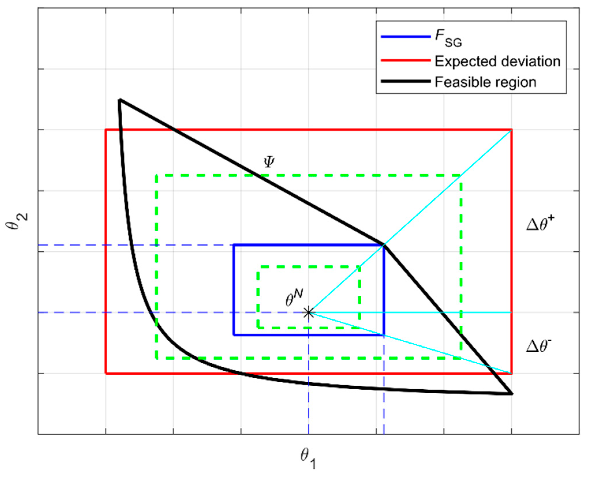
Let us define the general hyperrectangle:
With δ non-negative scalar variable for which
The flexibility index FSG, proposed by Swaney and Grossmann, is then the solution to the constrained optimization flexibility problem:
where d and z represent the design and the manipulated variables respectively. By referring to Figure 2, FSG graphically represents the maximum scale factor so that the corresponding hyperrectangle is bounded by the feasible zone. Moreover, for constraints jointly quasi-convex in z and 1D quasi-convex in θ, the solution lies at a vertex of the hyperrectangle allowing to solve the optimization problem by evaluating the feasibility of the design at each vertex. On the contrary, certain types of non-convex domains may lead to nonvertex solutions.
The index presented here above can be referred to as “deterministic” since it is based on the assessment of a “perturbation magnitude” in the uncertain domain without taking into account the perturbation likelihood. Thus, this index definition results in a rather conservative estimation of the system flexibility.
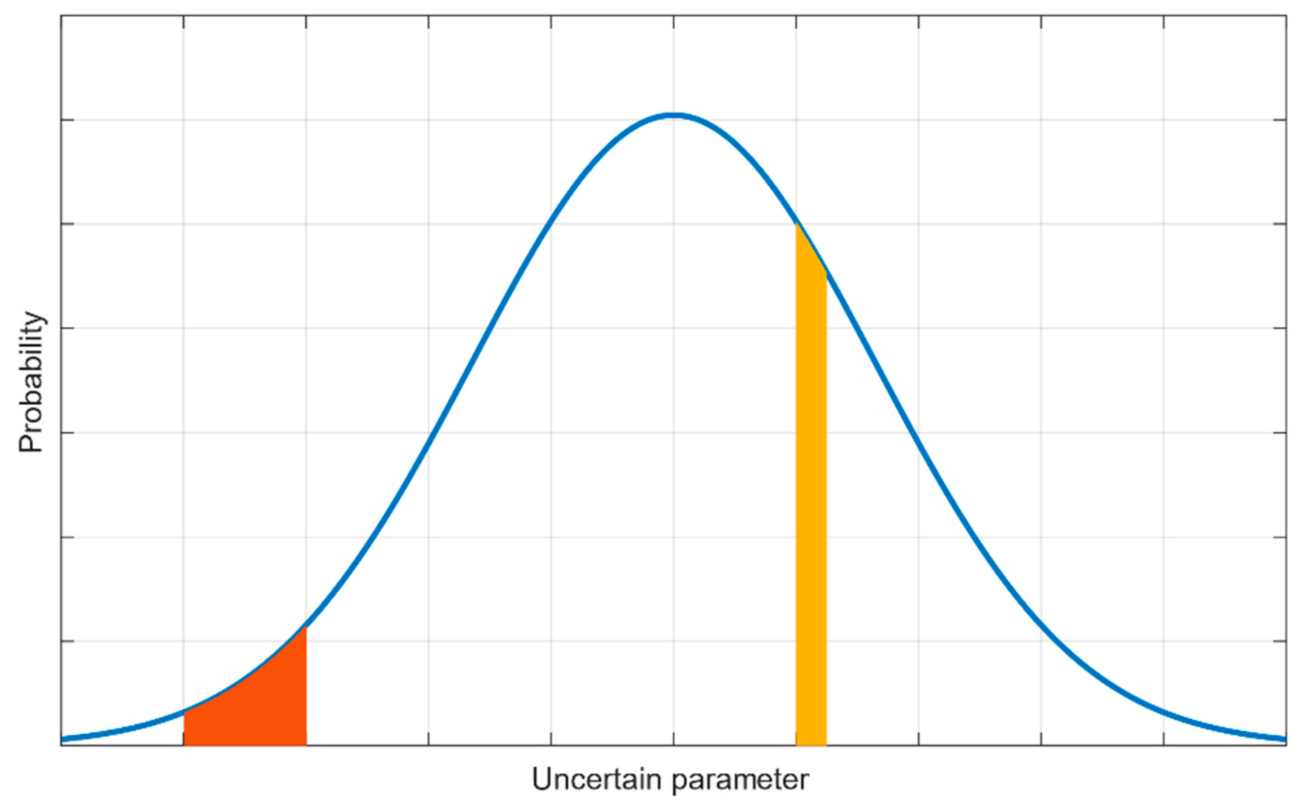
For these reasons, a few years later, Pistikopoulos and Mazzuchi (1990) [31] introduced a stochastic flexibility index based on the perturbation likelihood. Given the uncertain parameters Probability Distribution Function (hereafter PDF) P(θ) and the feasible region
the stochastic flexibility index SF can be defined as:
Unlike the deterministic indices, the stochastic flexibility one does not quantify a perturbation magnitude but assesses the percentage of the possible operating conditions for which the system keeps being feasible. However, the higher cost to pay for such an accurate result does not lie on the higher need for data only. As shown in Figure 3 indeed, more than one subregion in the uncertain domain corresponding to the same value of integral (11) could exist.
Therefore, the design choice and the related Time Average Losses (TAL, hereafter denoted by Θ) associated with each value of SF is the result of an economic optimization problem stated as:
where
This formulation states that, for each value SF of the stochastic flexibility index, the associated subregion D, represented by the maximum value of Θ in it, is the cheapest one among all the subregions satisfying the Equation (11). Thus, for each step of the stochastic flexibility analysis an additional optimization problem should be solved, considerably increasing the required computational effort.
The particular definition of this index makes it different from the deterministic ones by two main properties as pointed out by Di Pretoro et al. (2019) [13]:
- The stochastic flexibility index SF has always a value between 0 and 1;
- Under nominal operating conditions, SF can be higher than 0.
The importance of including flexibility when assessing operating costs has already been proved by Di Pretoro et al. (2020) [32]. However, in order to do that the decisional algorithm for the operation scheduling to which the flexibility indices will be applied should be thoroughly defined. For this reason, a detailed explanation will be discussed in the following section.
3.3. Decisional Algorithm for Operation Scheduling
Given the heat exchanger case study under analysis with the related cleaning techniques and the associated fouling kinetic model described in Section 2 and Section 3.1 respectively, the decisional algorithm for the cleaning operation schedule should give the answers to two main questions:
- WHEN the cleaning operation should be performed?
- WHICH cleaning operation should be performed?
In order to do that, some cost functions are required. The fact that the cycle is optimized with respect to an economic criterion implies that, once questions 1 and 2 are answered, a third question “what are the expected operating costs?” is answered as well.
The first cost function to use is called the “Energy Loss” function and it is defined as:
where CE is the cost per energy [€/J], t is the operating time, Qcl is the heat exchanged under clean conditions, i.e., at t = 0, and Q is the actual heat recovery at t = top. In particular, it can be observed that the integrated function represents the external heat duty demand, i.e., the sum between Qcold and Qhot. This cost function describes operating costs to be afforded when the heat recovery is still ongoing.
Two other cost functions should be defined in order to quantify the expenses incurring during the unit shutdown. The first one refers to the cost of the energy to be provided by the external duty when no heat recovery is performed. This value is equal to:
for solvent cleaning or
for mechanical cleaning where is the time required for the corresponding cleaning operation.
Finally, the last cost item is represented by the cost of the cleaning operation itself, abbreviated with and for the chemical and mechanical cleaning techniques respectively. The costs of cleaning have been assumed as constant in time. Although the code does not account for inflation and market trends’ influence, it is still possible to implement within it these aspects for real applications. However, this is not the purpose of this work.
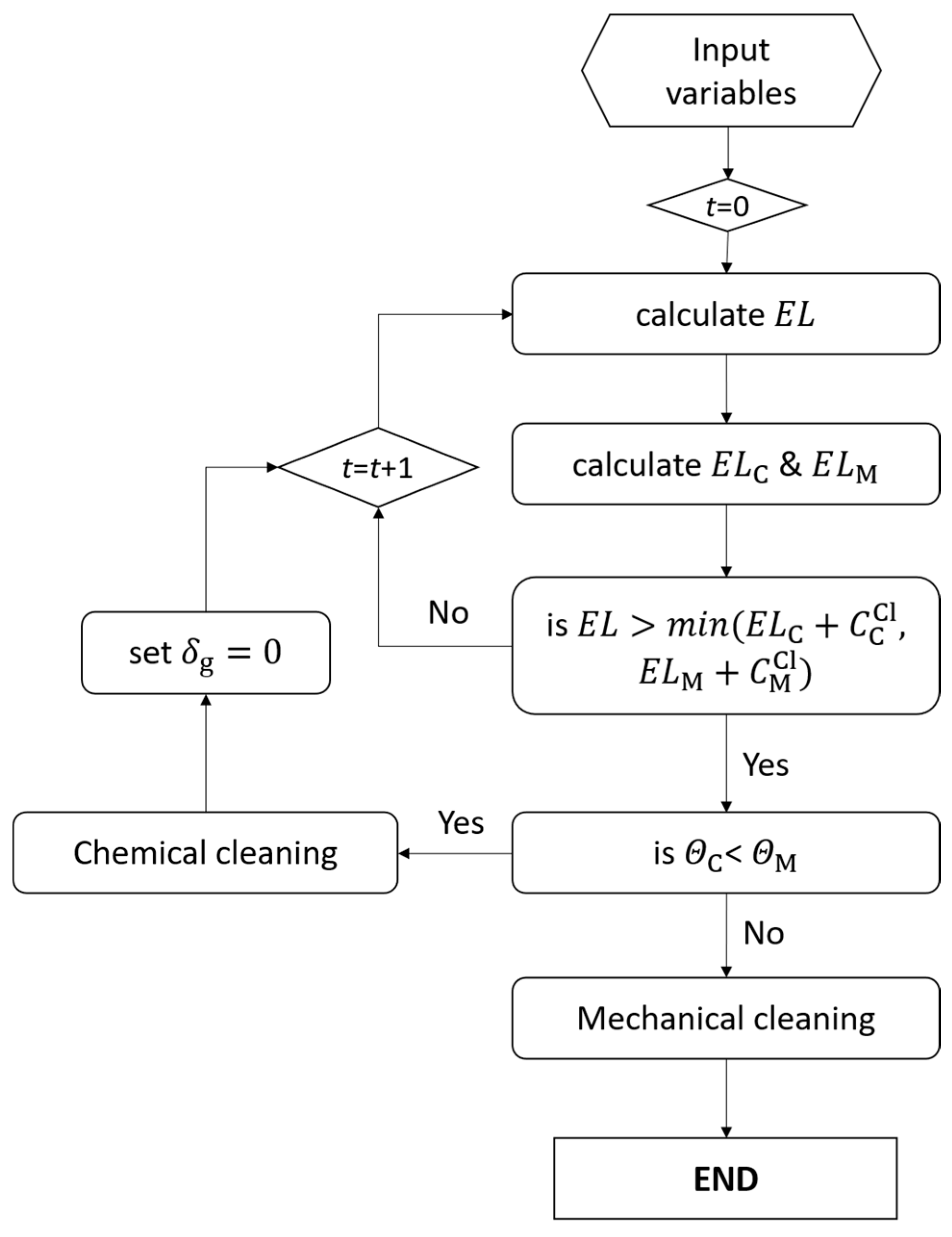
Once all these cost items are calculated, the optimization problem concerning the optimal cycle duration needs to be solved. Its general formulation is:
This formulation is used to solve the so-called supercycle, i.e., the sequence of multiple chemical cleaning operations (NC) required before performing the mechanical one. In particular, whether a cleaning operation is required, i.e., when the energy losses are higher than the cost of cleaning, the minimum value between ΘM and ΘC determines which kind of cleaning technique should be employed. In fact, each time the solvent cleaning is preferred, the coke layer keeps increasing until the chemical operation becomes more expensive than the mechanical one and the so-called supercycle is closed.
In the case where only mechanical cleaning is considered, the optimization problem is simplified by removing all the chemical cleaning related terms.
The decisional algorithm described here above has been graphically summarized in the flowchart reported in Figure 4.
The following section presents the obtained results both for the conventional procedure and for the stochastic flexibility based one. In the latter case, the economic optimization carried out to select the optimal scheduling has been coupled with the optimization required by the stochastic flexibility assessment. This innovative procedure allows outlining the trend of the cycle duration and the associated costs obtained from the first optimization as a function of the flexibility index resulting from the second one.
The heat exchanger and fouling models, the flexibility analysis, and the decisional algorithm for scheduling optimization calculations were all performed by means of MatLab® codes.
4. Results
The following sections present in detail the results obtained. In particular, they have been classified into three main parts. The first one shows the results of the scheduling algorithm applied to our case study under nominal operating conditions both in case of a single cleaning process and of the combination of the two.
A sensitivity analysis with respect to two possible uncertain variables will follow in order to detect the most critical one and use it to perform the flexibility assessment.
Finally, the third part presents and discusses in detail the outcome of the stochastic flexibility assessment for the single heat exchanger case study by coupling economic and operational aspects.
4.1. Nominal Operating Conditions
This section presents the results obtained with the process parameters discussed in Section 2 accounting both for the mechanical cleaning methodology only and for both chemical and mechanical ones.
4.1.1. Mechanical Cleaning Only
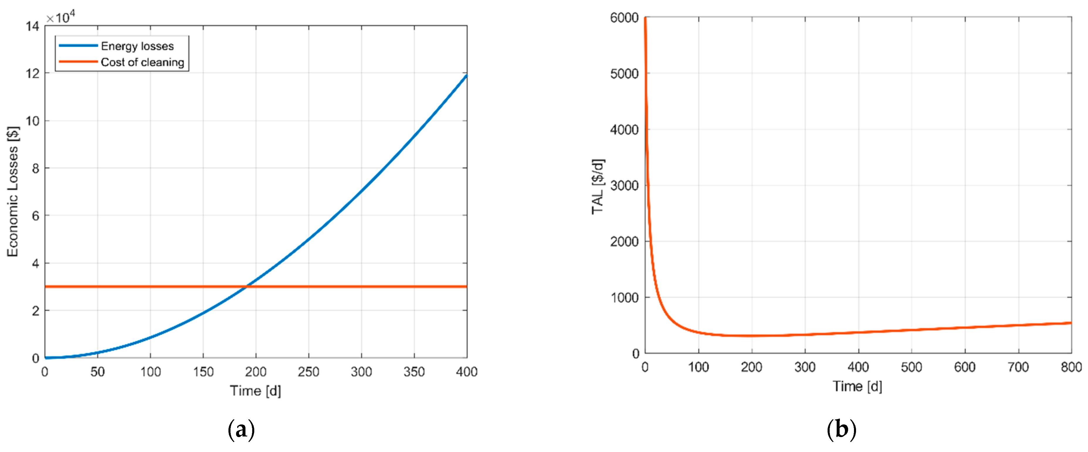
The scheduling optimization has been performed first according to the conventional methodology accounting for mechanical cleaning only. The time average losses have been calculated for a range of cycle time and the top corresponding to its minimum value has been detected.
The overall Energy Losses and the TAL trend as a function of the operation time are shown in Figure 5a,b respectively. As it can be noticed, for low top values, the TAL are very high since the cleaning costs are much higher than the cost of the external duty required to compensate for the lower performance of the heat exchanger due to the fouling phenomenon. This value decreases until a minimum of 306.16 $/d in correspondence of 195 days and starts increasing again for the longer top because of the higher impact of the EL with respect to the cleaning expenses.
4.1.2. Supercycle
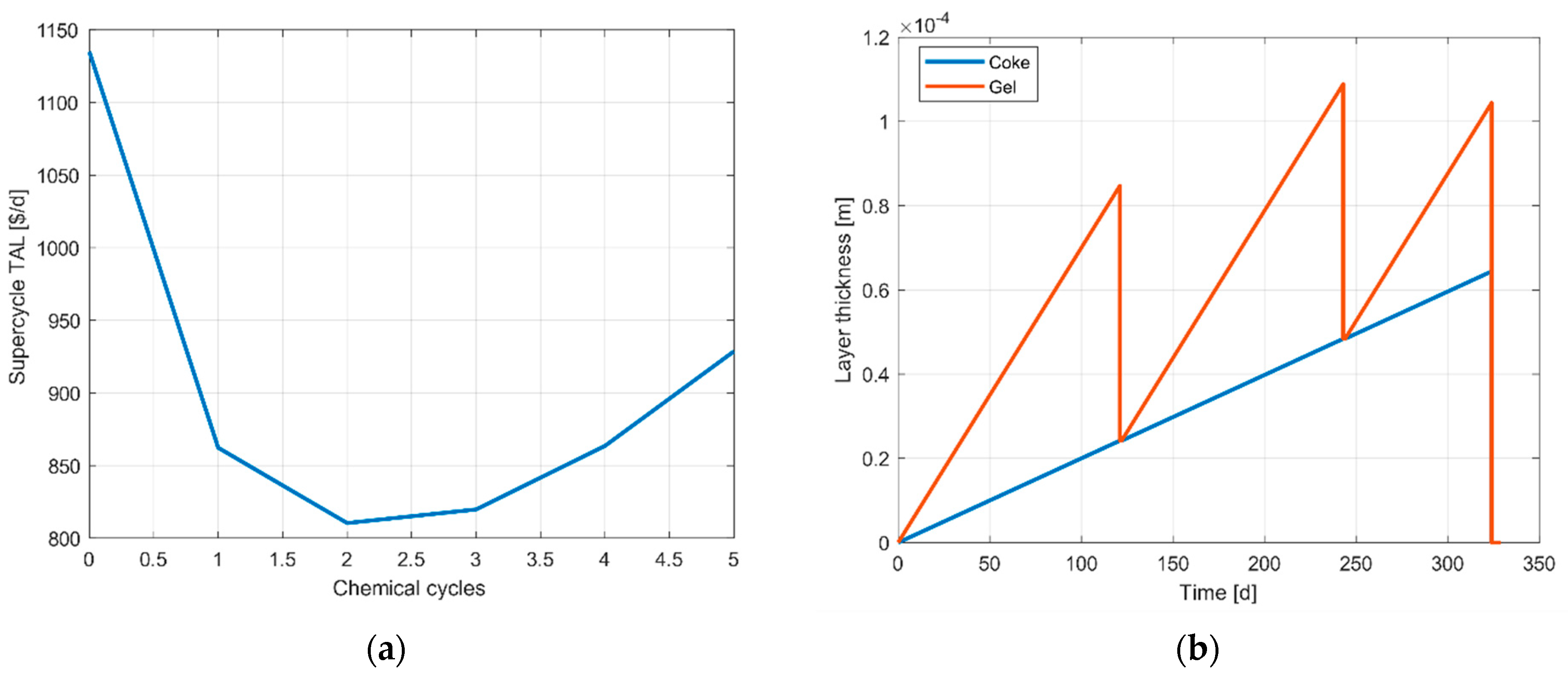
The decisional algorithm for scheduling optimization has been then applied accounting for both the gel and the coke layers according to the methodology presented in Section 3.3. The TAL cost function was evaluated for different numbers of chemical cleaning cycles NC before performing the mechanical operation.
Figure 6a shows the optimal TAL value for NC ranging from 0 to 5. The function in 0 represents the result obtained when no chemical cleaning is performed before the mechanical one. This value is exactly the one obtained for a simple cycle scheduling in the previous section, i.e., 306.16 $/d. The TAL trend shows a minimum of 234 $/d in correspondence of NC equal to 2. This means that the optimal supercycle consists of two chemical cleanings and a mechanical one. For lower values, i.e., 1 and 0, the energy losses due to the lower efficiency of the heat recovery do not justify the cost of a mechanical operation. On the other hand, for higher values, the impact of the increasing coke layer on the heat transfer implies substantial energy losses that would compromise the profitability of the operation more than the cost of complete cleaning.
In order to ease the understanding of this phenomenon, the gel and coke layer thicknesses as a function of time have been represented in Figure 6b for the optimal operation scheduling.
The time interval when the layer thickness has a stationary trend refers to cleaning operation time, i.e., the unit maintenance shutdown time. In particular, it can be noticed that the last shutdown required for the mechanical cleaning is longer than the previous ones (5 days vs. 1 day) due to the higher complexity related to the coke layer removal.
The most relevant outcome of this section is that the combination of two different cleaning strategies allows to save up to 24% of the time average losses thanks to the lower complexity and duration of the solvent cleaning subcycle.
4.2. Sensitivity Analysis
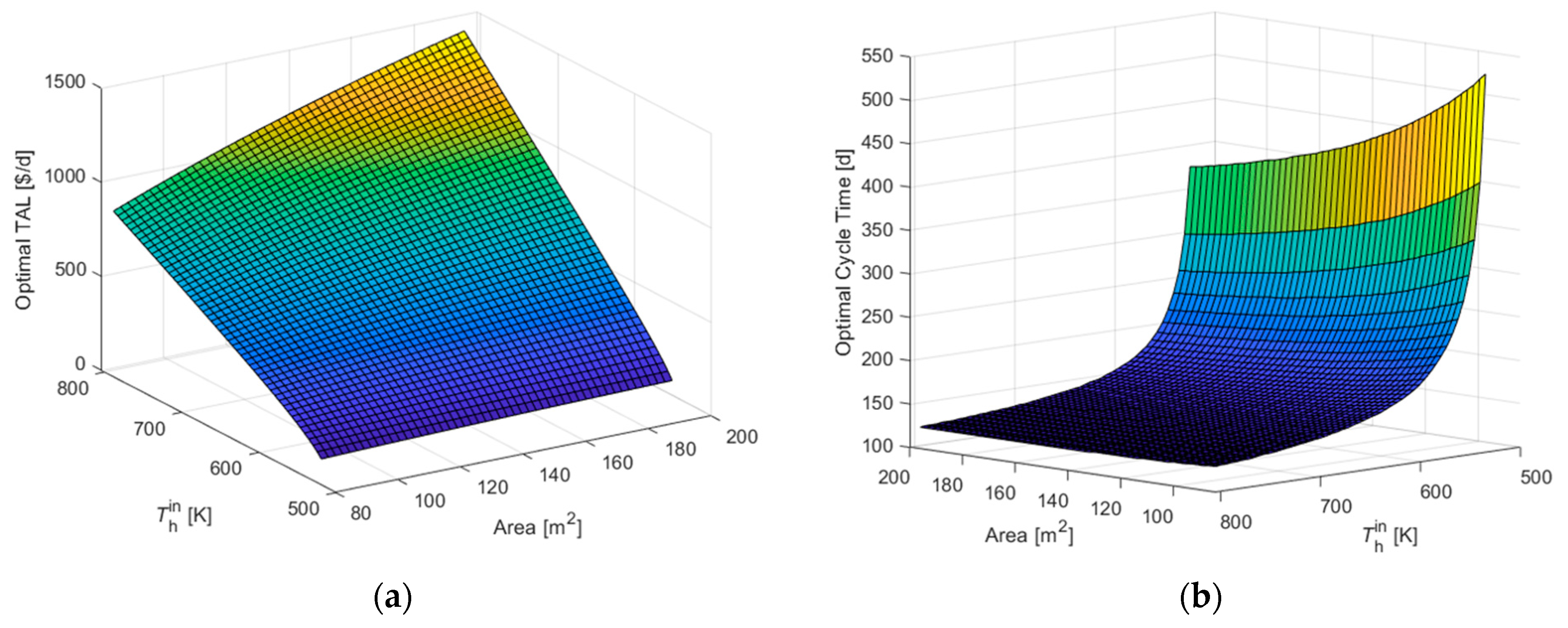
The sensitivity analysis was performed on the hot side inlet temperature and the heat transfer surface area A. The choice of perturbing both an input parameter and a design variable has the purpose to verify which one of them has a higher impact on the operation scheduling. The most critical one indeed will be selected as an uncertain parameter to perform the stochastic flexibility assessment.
Figure 7 shows the results of the sensitivity analysis for wide ranges of the perturbed variables. In particular, Figure 7a refers to the optimal cycle TAL while Figure 7b shows the corresponding optimal cycle time.
On the one hand, in the former Figure, an almost linear trend of the Time Average Losses as a function of the two perturbed variables can be noticed. More precisely, for the same deviation in terms of percentage, the TAL shows a slightly higher sensitivity with respect to than to A. In particular, the sensitivity of the cost function with respect to one of the two variables becomes more relevant as the value of the other one gets higher.
On the other hand, in the latter Figure, the higher sensitivity of the optimal cycle time with respect to the temperature results to be much more relevant. The perturbation of top with respect to the heat transfer surface area is almost negligible for low values and shows a moderate response for very high-temperature perturbations. On the contrary, the optimal cycle time exhibits an almost exponential growth with respect to the inlet temperature for any value of the heat transfer surface area. This behavior can be reconducted to the fact that this parameter directly acts on the external duty demand required to achieve the hot side specification while the heat exchanger was already properly sized and affects the optimal scheduling solution only in case of very ineffective heat transfer.
Thus, in the light of these results, the intermediate value A = 140 m2 was finally kept as the nominal one while the hot side inlet temperature has been selected as uncertain parameters for the flexibility analysis presented in detail in the next section.
4.3. Flexibility Assessment
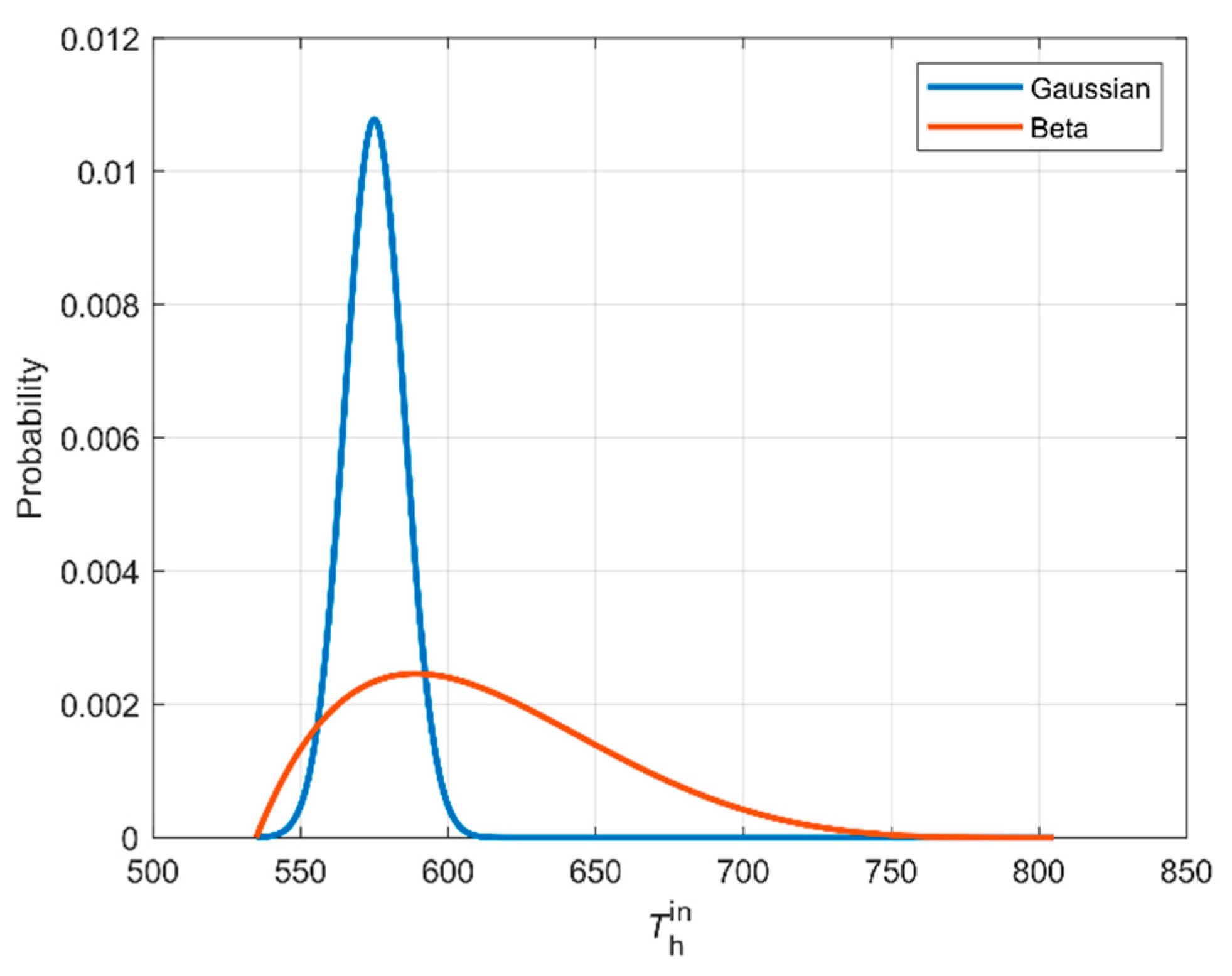
As already discussed in detail by previous studies dealing with the aleatory uncertainty and the stochastic flexibility index [13,31,32], the uncertainty characterization, i.e., the probability distribution function used to describe the uncertain parameter likelihood, plays a main role in the final result. For this reason, in order to have a more complete overview, two PDFs, namely the Gaussian and the Beta distributions, are employed in this study. The former describes an uncertain variable perturbation with a symmetric behavior with respect to the central point (i.e., its mode) usually corresponding to the nominal operating conditions. On the other hand, the Beta distribution defines an aleatory parameter for which either the positive or the negative deviation is more likely to occur. Further details about their mathematical formulation are provided in the Appendix A.
Both the Gaussian (or Normal) and the Beta distributions belong to the class of two-parameter PDFs, therefore two conditions should be imposed in order to uniquely determine their trends. In the case of real applications, the distribution of the uncertain parameter can be outlined according to the available frequency data or accounting for its expected behavior. For this paper, since the study is not related to any existing unit, the maximum likelihood of the PDF was set equal to the nominal operating conditions point and the variance was selected so that the entire uncertain space is covered with a residual probability lower than the 0.01%.
The trends resulting from these hypotheses have been outlined in Figure 8. As it can be noticed, the Gaussian distribution results particularly narrow with respect to the entire temperature range since there is a minimum inlet temperature below which the heat transfer is not feasible due to a minimum temperature approach lower than 10 °C. This value was then set as the lower boundary of the uncertain domain.
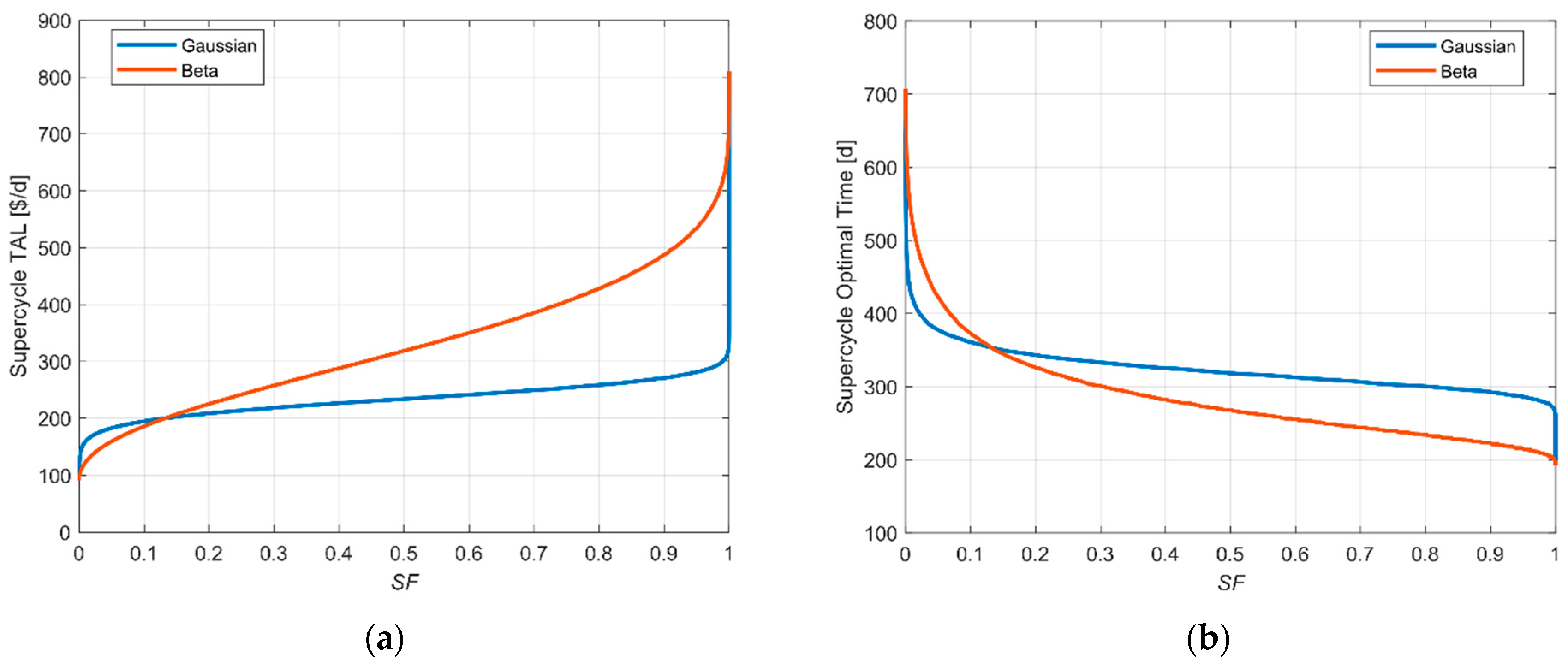
Once the uncertain parameter PDF has been properly defined, the stochastic flexibility assessment can be finally carried out according to the methodology presented in Section 3.2. Each probability distribution function was then integrated over the uncertain domain and the maximum TAL and cycle time have been assessed at each value of the SF index. This procedure allowed to estimate the expected costs and operation time to be respectively afforded and waited for each simple cycle.
The cost trends obtained this way are shown in Figure 9. As it can be noticed, the expected TAL grows fast for very low flexibility index values until a lower slope increased is attained over a wide range of the uncertain parameter. As the residual probability gets lower, much higher losses should be expected in order to almost entirely cover the uncertain domain.
The interval width reflects the PDF shape as expected and has already been discussed in the previous sections. In particular, the “steady” region is much wider in the case of the Gaussian one. The TAL for lower values resulted higher for the Beta PDF while the cost increase in the residual part of the stochastic flexibility index is more relevant when using the Gaussian one.
In regards to the optimal cycle time, the obtained curves show an opposite trend with respect to the corresponding TAL functions. This behavior is due to the fact that higher inlet temperature requires cleaning cycles to be more frequently performed as already pointed out by the sensitivity analysis. Analogously to the economic remarks discussed in Section 4.1.2 about the costs, the use of a combined chemical and mechanical cleaning methodology allows extending the operating time before a complete shutdown is required.
In any case, the two trends are qualitatively similar. It is worth remarking that the presence of some edges in these trends is due to the discretization of the uncertain domain that was not kept too dense in order to avoid excessive computational time.
The same procedure was then carried out for the supercycle accounting for both chemical and mechanical cleaning operations.
The optimal number of solvent cleaning cycles over the uncertain domain always resulted as 2. However, the corresponding costs and optimal cycle time considerably vary over the inlet temperature interval as shown by the plots in Figure 10a,b for the two probability distributions. Given that the optimal supercycle configuration does nott change, relatively smooth trends can be observed for both the output variables and both the PDFs without any particular discontinuous point. As for the simple cycle, a fast increase in the cost function can be observed for very low and very high SF values. However, for the supercycle, the Beta distribution exhibits a higher slope in the intermediate range with respect to the Gaussian one.
Even in this case, an opposite trend can be detected for the optimal cycle time as for the previous analysis. In general, higher costs, and thus lower optimal cycle time, can be pointed out for the Beta distribution due to its higher variance.
Therefore, in the light of these results, it can be also concluded that, in the case of a narrow probability distribution, the scheduling parameters obtained accounting for nominal operating conditions only are much closer to the real estimation. This is due to the fact that the trends TAL and top vs. SF exhibit a lower slope over a wider flexibility range and just the very last part of residual probability significantly affects their values.
5. Conclusions
The purpose of this research work was to include the uncertainty of the operating condition in the heat cleaning cycles scheduling optimization algorithm. The outcome of the study was successful and allowed for the definition of a thorough procedure to be applied in the case of heat exchanger cleaning cycle optimal scheduling.
The general validity of the innovative algorithm with respect to the uncertainty characterization was proved by testing both a symmetric (i.e., Gaussian) and a skewed (i.e., Beta) probability distribution function. Moreover, the procedure does not depend on the fouling kinetic model that is used to describe the physical phenomena related to fouling.
Furthermore, the employment of a preliminary sensitivity analysis is proposed in this study with the purpose of restraining the number of uncertain parameters to be accounted for by identifying the most critical ones from a flexibility perspective and thus decreasing the dimension of the uncertain domain.
A further result obtained during this study was the algorithm aimed at the optimally combined solvent and mechanical cleaning cycle under uncertainty. As for nominal operating conditions, the possibility to exploit different cleaning operations allows reducing the costs related to fouling removal. However, the optimization of the so-called “supercycle” implies the introduction of an additional decisional variable, i.e., chemical vs. mechanical, requiring a non-negligible computational effort already in the case of a single unit.
In conclusion, a general procedure for operation scheduling under uncertainty was outlined by means of a stochastic flexibility indicator and, in particular, its application to a single heat exchanger cleaning cycle was analyzed in deep. The aleatory uncertainty characterization by means of a probability distribution function combined with the proposed algorithm provides a tool to the decision-maker to have a more reliable cost estimation and to define the best scheduling solution according to the specific operating conditions.
This work sets the basis for future applications on more complex heat exchanger networks as well as additional perspectives on other kinds of operations different than unit maintenance. Moreover, besides the use of the methodology proposed in this research study to deal with an undesired disturbance, i.e., fouling, the scheduling algorithm could be also actively exploited to take advantage of certain operational parameters in order to reduce operating costs and enhance the process performances.
Author Contributions
Conceptualization, A.D.P.; Data curation, F.D.; Methodology, A.D.P. and F.D.; Supervision, F.M.; Writing—original draft, A.D.P. and F.D. All authors have read and agreed to the published version of the manuscript.
Funding
This research received no external funding.
Institutional Review Board Statement
Not applicable.
Informed Consent Statement
Not applicable.
Data Availability Statement
Data sharing not applicable.
Conflicts of Interest
The authors declare no conflict of interest.
Glossary
| Symbol | Definition | Unit |
| A | Heat transfer surface area | m2 |
| CAPEX | CAPital EXpenses | $/a |
| Specific heat at constant pressure | J/(kg K) | |
| Cleaning costs | $ | |
| CE | Energy costs | $/J |
| D | Stochastic Flexibility index domain | n-D space |
| d | Design variable | variable |
| EL | Energy Losses | $ |
| FSG | Swaney & Grossmann flexibility index | 1 |
| GNP | Gross National Product | acronym |
| Ki | Fouling kinetic constant | (m2 K)/J |
| NC | Number of chemical cleaning cycles | 1 |
| OPEX | OPerating EXpenses | $/a |
| Probability Distribution Function | function | |
| P(θ) | Probability function | function |
| qm,i | Mass flow rate | kg/s |
| Qi | Heat duty | W |
| Rf | Fouling heat transfer resistance | (m2 K)/W |
| SF | Stochastic Flexibility index | 1 |
| t | Time | d |
| top | Operation time | d |
| T | Flexibility hyper-rectangle | function |
| TAL | Time Average Losses | acronym |
| Tin | Inlet temperature | K |
| U | Heat transfer coefficient | W/(m2 K) |
| z | Control variable | variable |
| Greek letters | ||
| α | Beta distribution shape parameter | 1 |
| β | Beta distribution scale parameter | 1 |
| δ | Flexibility index scale factor | 1 |
| δi | Fouling layer | m |
| Θ | Time Average Losses | $/d |
| θ | Uncertain variable | various |
| λi | Thermal conductivity | W/(m2 K) |
| μ | Mean | various |
| σ | Variance | various |
| τi | Cleaning time | d |
| Φi | Fouling deposition/removal rate | (m2 K)/W |
| Ψ | Feasible domain | n-D space |
Appendix A
The formulation of the probability distribution functions employed to describe the uncertain variable deviation likelihood will be discussed in detail here below in order to provide a better understanding of the associated mathematical properties. For further details please refer to Severini (2011) [33].
Appendix A.1. Normal Probability Distribution Function
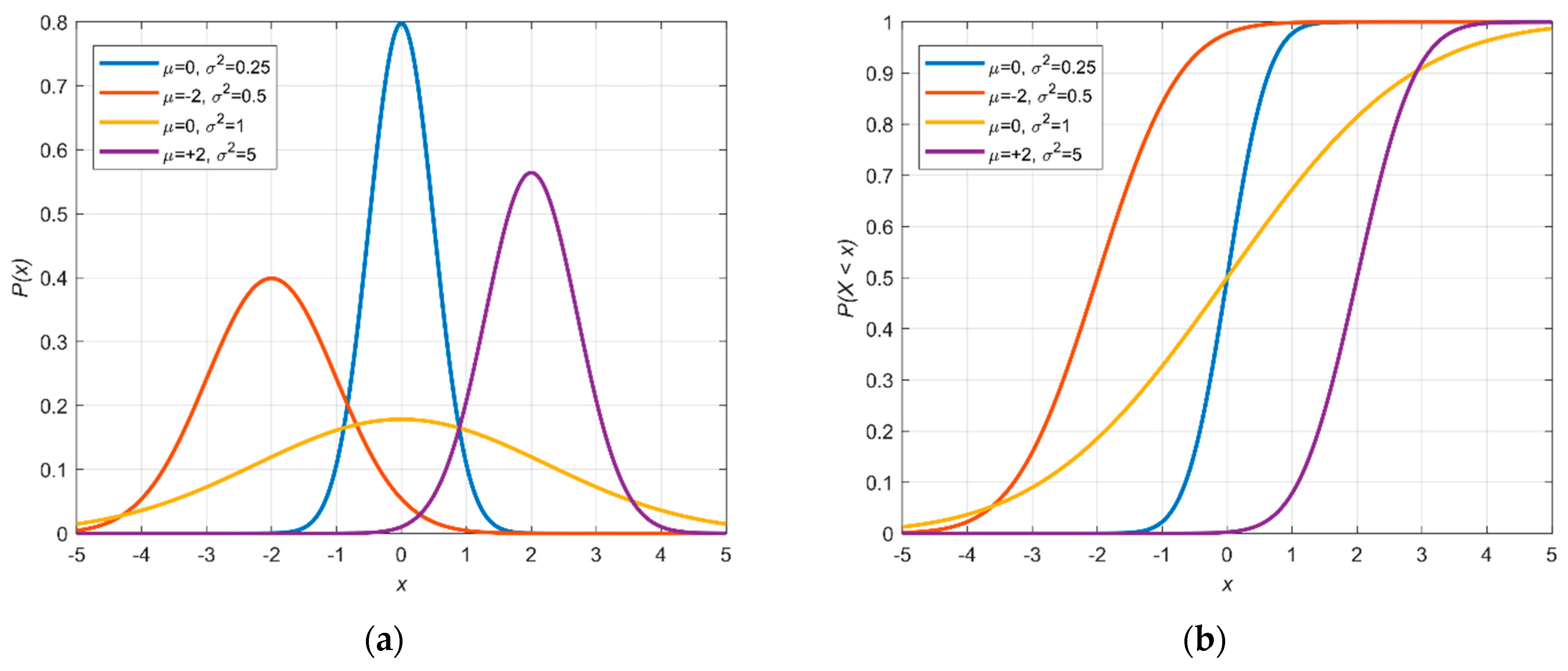
As already mentioned, the condition of “general validity” is represented by the Gaussian or normal probability distribution function. It is symmetrical with respect to its mean and the 99.73% of cumulative probability falls in the range ±3 times the variance [−3σ, +3σ].
Different Gaussian distributions are plotted in Figure A1 for different values of the characteristic parameters μ and σ.
Figure A1.
Normal (Gaussian) distribution: (a) Probability & (b) Cumulative Distribution Functions.

The single variable Normal PDF mathematical formulation states as:
where μ is the mean and σ is the variance.
For a general number of variables the n-variables normal PDF with can be defined as:
where Σ is the variance-covariance matrix, Σ−1 its inverse and |Σ| its determinant.
Moreover we can standardize, i.e., reconduct to a 0 mean value and variance equal to 1 (variance-covariance matrix equal to the identity matrix), the normal distribution by mean of the independent variable substitution:
obtaining:
for a general n variables standard normal probability distribution.
This transformation besides making the calculations easier allows to compare variables with different dimensions, e.g., temperature vs. flowrate vs. velocity etc.
The boundaries of the feasibility domain, if analytically available, have then to be rewritten as functions of the new variable z by inverting the Equation (A3).
Appendix A.2. Beta Probability Distribution Function
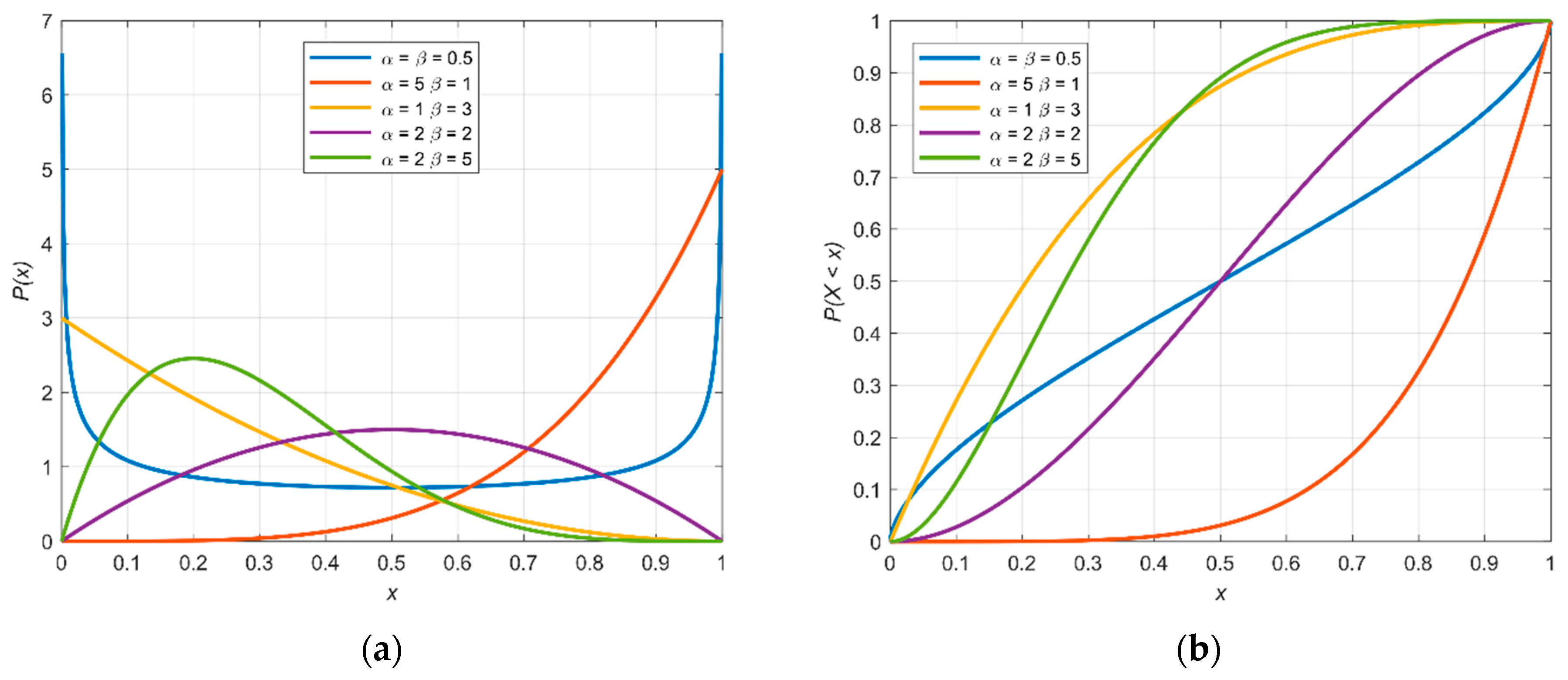
The second distribution function used in this paper to describe the uncertain variable deviation likelihood is the so called Beta PDF. It is a two-parameter continuous probability distribution defined for positive values of the independent variable x .
Beta distribution is defined according to two parameters; the parametrization with a shape parameter α and a scale parameter β is used here below. Different Gaussian distributions are plotted in Figure A2 for different values of the characteristic parameters.
Figure A2.
Beta distribution: (a) Probability & (b) Cumulative Distribution Functions.

The analytical expression of the single variable Beta PDF is formulated as:
The mode with α, β > 1 assumes the meaning of the most likely value of the distribution, it graphically corresponds to the peak in the PDF and is mathematically formulated as:
For α, β < 1 the behavior is opposite and is defined as the anti-mode, or the lowest point of the probability density curve.
For α = β, the expression for the mode simplifies to 1/2, showing that for α = β > 1 the mode (respectively anti-mode when α, β < 1), is at the center of the distribution: it is symmetric in those cases as can be seen in the figure.
References
- Pritchard, A.M. The Economics of Fouling. In Fouling Science and Technology; Melo, L.F., Bott, T.R., Bernardo, C.A., Eds.; NATO ASI Series; Springer: Dordrecht, The Netherlands, 1988; pp. 31–45. [Google Scholar] [CrossRef]
- Steinhagen, R.; Müller-Steinhagen, H.; Maani, K. Problems and Costs due to Heat Exchanger Fouling in New Zealand Industries. Heat Transf. Eng. 1993, 14, 19–30. [Google Scholar] [CrossRef]
- Awad, M.M. Fouling of Heat Transfer Surfaces. Chem. Eng. Technol. 2011. [Google Scholar] [CrossRef] [Green Version]
- Bott, T.R. Fouling of Heat Exchangers, 1st ed.; Elsevier Science: Amsterdam, The Netherlands; New York, NY, USA, 1995. [Google Scholar]
- Pogiatzis, T.; Ishiyama, E.M.; Paterson, W.R.; Vassiliadis, V.S.; Wilson, D.I. Identifying optimal cleaning cycles for heat exchangers subject to fouling and ageing. Appl. Energy 2012, 89, 60–66. [Google Scholar] [CrossRef]
- Méndez, C.A.; Cerdá, J.; Grossmann, I.E.; Harjunkoski, I.; Fahl, M. State-of-the-art review of optimization methods for short-term scheduling of batch processes. Comput. Chem. Eng. 2006, 30, 913–946. [Google Scholar] [CrossRef] [Green Version]
- Mockus, L.; Reklaitis, G.V. A New Global Optimization Algorithm for Batch Process Scheduling. In State of the Art in Global Optimization; Nonconvex Optimization and Its Applications; Floudas, C.A., Pardalos, P.M., Eds.; Springer: Boston, MA, USA, 1996; Volume 7, pp. 521–538. [Google Scholar]
- Xueya, Z.; Sargent, R.W.H. A new unified formulation for process scheduling. In Proceedings of the AIChE Annual Meeting, Paper No. 144c, St. Louis, MO, USA, 7–12 November 1993. [Google Scholar]
- Stefanis, S.; Livingston, A.; Pistikopoulos, E. Environmental impact considerations in the optimal design and scheduling of batch processes. Comput. Chem. Eng. 1997, 21, 1073–1094. [Google Scholar] [CrossRef]
- Grau, R.; Graells, M.; Corominas, J.; Espuña, A.; Puigjaner, L. Global strategy for energy and waste analysis in scheduling and planning of multiproduct batch chemical processes. Comput. Chem. Eng. 1996, 20, 853–868. [Google Scholar] [CrossRef]
- Di Pretoro, A.; Montastruc, L.; Manenti, F.; Joulia, X. Exploiting Residue Curve Maps to Assess Thermodynamic Feasibility Boundaries under Uncertain Operating Conditions. Ind. Eng. Chem. Res. 2020, 59, 16004–16016. [Google Scholar] [CrossRef]
- Hoch, P. Evaluation of design flexibility in distillation columns using rigorous models. Comput. Chem. Eng. 1995, 19, S669–S674. [Google Scholar] [CrossRef]
- Di Pretoro, A.; Montastruc, L.; Manenti, F.; Joulia, X. Flexibility analysis of a distillation column: Indexes comparison and economic assessment. Comput. Chem. Eng. 2019, 124, 93–108. [Google Scholar] [CrossRef] [Green Version]
- Sudhoff, D.; Leimbrink, M.; Schleinitz, M.; Gorak, A.; Lutze, P. Modelling, design and flexibility analysis of rotating packed beds for distillation. Chem. Eng. Res. Des. 2015, 94, 72–89. [Google Scholar] [CrossRef]
- Adams, T.A.; Thatho, T.; Le Feuvre, M.C.; Swartz, C.L.E. The Optimal Design of a Distillation System for the Flexible Polygeneration of Dimethyl Ether and Methanol under Uncertainty. Front. Energy Res. 2018, 6, 41. [Google Scholar] [CrossRef] [Green Version]
- Floudas, C.A.; Gümüş, A.Z.H. Global Optimization in Design under Uncertainty: Feasibility Test and Flexibility Index Problems. Ind. Eng. Chem. Res. 2001, 40, 4267–4282. [Google Scholar] [CrossRef]
- Huang, W.; Yang, G.; Qian, Y.; Jiao, Z.; Dang, H.; Qiu, Y.; Cheng, Z.; Fan, H. Operation Feasibility Analysis of Chemical Batch Reaction Systems with Production Quality Consideration under Uncertainty. J. Chem. Eng. Jpn. 2017, 50, 45–52. [Google Scholar] [CrossRef] [Green Version]
- Balasubramanian, J.; Grossmann, I.E. A novel branch and bound algorithm for scheduling flow shop plants with uncertain processing times. Comput. Chem. Eng. 2002, 26, 41–57. [Google Scholar] [CrossRef]
- Balasubramanian, J.; Grossmann, I.E. Scheduling optimization under uncertainty—An alternative approach. Comput. Chem. Eng. 2002, 27, 469–490. [Google Scholar] [CrossRef]
- Bonfill, A.; Espuña, A.; Puigjaner, L. Addressing Robustness in Scheduling Batch Processes with Uncertain Operation Times. Ind. Eng. Chem. Res. 2005, 44, 1524–1534. [Google Scholar] [CrossRef]
- Smaili, F.; Angadi, D.; Hatch, C.; Herbert, O.; Vassiliadis, V.; Wilson, D. Optimization of Scheduling of Cleaning in Heat Exchanger Networks Subject to Fouling. Food Bioprod. Process. 1999, 77, 159–164. [Google Scholar] [CrossRef]
- Diaby, A.L.; Miklavcic, S.; Addai-Mensah, J. Optimization of scheduled cleaning of fouled heat exchanger network under ageing using genetic algorithm. Chem. Eng. Res. Des. 2016, 113, 223–240. [Google Scholar] [CrossRef]
- Dias, L.S.; Ierapetritou, M.G. Integration of scheduling and control under uncertainties: Review and challenges. Chem. Eng. Res. Des. 2016, 116, 98–113. [Google Scholar] [CrossRef]
- Ishiyama, E.; Paterson, W.R.; Wilson, D.I. Optimum cleaning cycles for heat transfer equipment undergoing fouling and ageing. Chem. Eng. Sci. 2011, 66, 604–612. [Google Scholar] [CrossRef]
- Sinnott, R.K.; Towler, G. Chemical Engineering Design, 6th ed.; Butterworth-Heinemann: Waltham, MA, USA, 2019. [Google Scholar]
- Wenner, R.R. Thermochemical Calculations, 1st ed.; McGraw-Hill Book Co.: New York, NY, USA; London, UK, 1941. [Google Scholar]
- Green, D.; Perry, R.; Southard, M.Z. Perry’s Chemical Engineers’ Handbook, 9th ed.; McGraw-Hill Education: New York, NY, USA, 2019. [Google Scholar]
- Hall, S.M. Rules of Thumb for Chemical Engineers, 4th ed.; Gulf Professional Publishing: Houston, TX, USA, 2011. [Google Scholar]
- Hoch, P.; Eliceche, A.M. Flexibility analysis leads to a sizing strategy in distillation columns. Comput. Chem. Eng. 1996, 20, S139–S144. [Google Scholar] [CrossRef]
- Swaney, R.E.; Grossmann, I.E. An index for operational flexibility in chemical process design. Part I: Formulation and theory. AIChE J. 1985, 31, 621–630. [Google Scholar] [CrossRef]
- Pistikopoulos, E.; Mazzuchi, T. A novel flexibility analysis approach for processes with stochastic parameters. Comput. Chem. Eng. 1990, 14, 991–1000. [Google Scholar] [CrossRef]
- Di Pretoro, A.; Montastruc, L.; Manenti, F.; Joulia, X. Flexibility assessment of a biorefinery distillation train: Optimal design under uncertain conditions. Comput. Chem. Eng. 2020, 138, 106831. [Google Scholar] [CrossRef]
- Severini, T.A. Elements of Distribution Theory; Cambridge University Press (CUP): Cambridge, UK, 2005. [Google Scholar]
Figure 1.
Heat exchanger system layout.

Figure 2.
Flexibility representation on the uncertain domain.

Figure 3.
Stochastic flexibility index SF representation on a Normal Probability Distribution Function (PDF).
Figure 3.
Stochastic flexibility index SF representation on a Normal Probability Distribution Function (PDF).

Figure 4.
Decisional algorithm.

Figure 5.
Mechanical cleaning: (a) Energy Losses and Cleaning Costs vs. cycle time; (b) Time Average Losses (TAL) vs. cycle time.
Figure 5.
Mechanical cleaning: (a) Energy Losses and Cleaning Costs vs. cycle time; (b) Time Average Losses (TAL) vs. cycle time.

Figure 6.
Supercycle optimal scheduling: (a) TAL vs. number of solvent cleaning NC; (b) Supercycle layer thickness trend.
Figure 6.
Supercycle optimal scheduling: (a) TAL vs. number of solvent cleaning NC; (b) Supercycle layer thickness trend.

Figure 7.
Sensitivity analysis results: (a) Optimal cycle TAL; (b) Optimal cycle time.

Figure 8.
Hot inlet temperature probability distribution.

Figure 9.
Flexibility analysis results—mechanical cleaning: (a) Optimal cycle TAL vs. SF; (b) Optimal cycle time vs. SF.
Figure 9.
Flexibility analysis results—mechanical cleaning: (a) Optimal cycle TAL vs. SF; (b) Optimal cycle time vs. SF.

Figure 10.
Flexibility analysis results—supercycle: (a) Optimal supercycle TAL vs. SF; (b) Optimal supercycle time vs. SF.
Figure 10.
Flexibility analysis results—supercycle: (a) Optimal supercycle TAL vs. SF; (b) Optimal supercycle time vs. SF.


Table 1.
Fouling vs. Gross National Product (GNP) (2018).
| Country | Costs (M$/a) | GNP 2018 (M$/a) | Costs/GNP (%) |
|---|---|---|---|
| US | 14,175 | 20,891,000 | 0.13% |
| Germany | 4875 | 4,356,353 | 0.21% |
| France | 2400 | 2,962,799 | 0.15% |
| Japan | 10,000 | 5,594,452 | 0.33% |
| Australia | 463 | 1,318,153 | 0.06% |
| New Zealand | 64.5 | 197,827 | 0.06% |
Table 2.
Process parameters.
| Symbols | Quantities | Value | Unit | |
|---|---|---|---|---|
| Heat exchanger | Overall heat transfer coefficient | 350 | W/(m2 K) | |
| Surface area | 140 | m2 | ||
| Cold stream | Mass flow rate | 135 | kg/s | |
| Inlet temperature | 525 | K | ||
| Specific heat capacity | 3125 | J/(kg K) | ||
| Hot stream | Mass flow rate | 68 | kg/s | |
| Inlet temperature | 575 | K | ||
| Specific heat capacity | 2200 | J/(kg K) | ||
| Fouling | Deposition rate | 5 × 10⁻⁶ | (m2 K)/(W d) | |
| Ageing rate | 2.5 × 10⁻⁷ | (m2 K)/(W d) | ||
| Gel thermal conductivity | 0.1 | W/(m K) | ||
| Coke thermal conductivity | 0.8 | W/(m K) |
Publisher’s Note: MDPI stays neutral with regard to jurisdictional claims in published maps and institutional affiliations. |
© 2021 by the authors. Licensee MDPI, Basel, Switzerland. This article is an open access article distributed under the terms and conditions of the Creative Commons Attribution (CC BY) license (http://creativecommons.org/licenses/by/4.0/).
Share and Cite
MDPI and ACS Style
Di Pretoro, A.; D’Iglio, F.; Manenti, F. Optimal Cleaning Cycle Scheduling under Uncertain Conditions: A Flexibility Analysis on Heat Exchanger Fouling. Processes 2021, 9, 93. https://0-doi-org.brum.beds.ac.uk/10.3390/pr9010093
AMA Style
Di Pretoro A, D’Iglio F, Manenti F. Optimal Cleaning Cycle Scheduling under Uncertain Conditions: A Flexibility Analysis on Heat Exchanger Fouling. Processes. 2021; 9(1):93. https://0-doi-org.brum.beds.ac.uk/10.3390/pr9010093
Chicago/Turabian StyleDi Pretoro, Alessandro, Francesco D’Iglio, and Flavio Manenti. 2021. "Optimal Cleaning Cycle Scheduling under Uncertain Conditions: A Flexibility Analysis on Heat Exchanger Fouling" Processes 9, no. 1: 93. https://0-doi-org.brum.beds.ac.uk/10.3390/pr9010093
Note that from the first issue of 2016, this journal uses article numbers instead of page numbers. See further details here.