Research of Flow Stability of Non-Newtonian Magnetorheological Fluid Flow in the Gap between Two Cylinders ^†

Abstract

This paper deals with a mathematical modeling of flow stability of Newtonian and non-Newtonian fluids in the gap between two concentric cylinders, one of which rotates. A typical feature of the flow is the formation of a vortex flow, so-called Taylor vortices. Vortex structures are affected by the speed of the rotating cylinder and the physical properties of the fluids, i.e., viscosity and density. Analogy in terms of viscosity is assumed for non-Newtonian and magnetorheological fluids. Mathematical models of laminar, transient and turbulent flow with constant viscosity and viscosity as a function of the deformation gradient were formulated and numerically solved to analyze the stability of single-phase flow. To verify them, a physical experiment was performed for Newtonian fluids using visualizations of vortex structures—Taylor vortices. Based on the agreement of selected numerical and physical results, the experience was used for numerical simulations of non-Newtonian magnetorheological fluid flow.

1. Introduction

Immiscible liquids are specified as a system of two (or more) components, e.g., liquid–liquid or liquid–solid phase. The solid phase is represented by particles dispersed in the carrier fluid. Their interaction in the flow depends on their chemical composition and physical properties. In case of magnetorheological fluids, we must account for the influence of the magnetic field, which can change the Newtonian viscosity to a non-Newtonian one [1,2,3,4,5,6].

Viscosity is considered constant for Newtonian fluids. For non-Newtonian and magnetorheological fluids, it depends on the deformation gradient [2,6,7,8,9]. Non-Newtonian fluids are widely used in the industry, especially in the hydraulic gaps of rotary machines. The use of magnetorheological fluid and ferrofluid has recently been investigated in the application of hydraulic lubrication.

The aim of this work is to define and verify the mathematical model for laminar, transient and turbulent flow for non-Newtonian and magnetorheological fluids in the gap between two concentric cylinders. The flow in the annulus is closely connected with practical applications. In addition, the flow is mostly laminar, so attention is focused on the study of laminar, transient and incipient turbulent flow.

The flow of non-Newtonian fluids has many other industrial applications. It has been investigated mainly in connection with laminar flow in various geometries [10], in porous media [11], in pipelines and hydraulic lubrication gaps [12], in chemical industry [13] and others. At present, magnetorheological fluids can be also included in this category. These fluids are mostly a suspension of metal particles with a diameter of the order of several μm dispersed in the carrier fluid (water or oil).

These fluids change their physical properties under the action of a magnetic field of various intensities. The fluid, in terms of viscosity originally of the Newtonian type, changes to a non-Newtonian fluid. The viscosity depends nonlinearly on the shear strain rate. There are many rheological models, which are used to approximate the rheogram of non-Newtonian fluids to some degree, such as the Bingham, power law, Carreau and Herschel–Bulkley, but they do not capture the nature of viscosity in the required range of applications. It is recommended to determine the viscosity by experimental measurements.

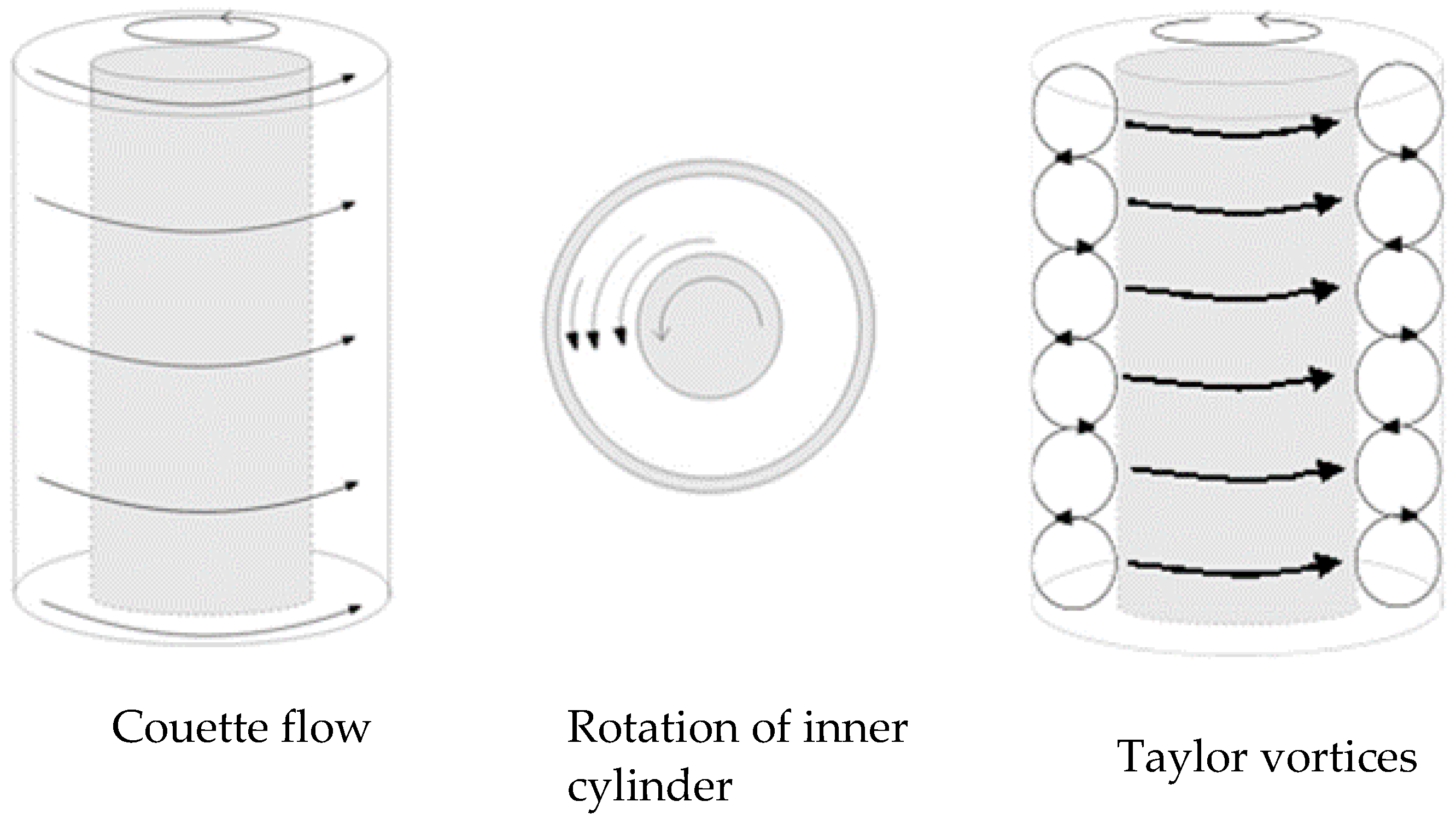
Mathematical models of the transient flow between the laminar and turbulent regime are problematic, especially in areas with the formation of vortex structures. These structures can be well observed in the gaps between the rotating cylinders (see Figure 1).

In laminar and transient flow, Couette flow without vortex structures can be observed. With increasing the rotational speed of the cylinder, stable Taylor vortices form, then the vortices change to wave mode, spiral mode, etc. In turbulent mode, vortices are formed analogous to stable vortices. Variants of vortex structures can be investigated by stability methods applied to mathematical models and evaluated by stability diagrams [14,15,16].

With the development of mathematical models of turbulence, a few flow models have been developed. Their correctness in the case of Taylor vortices is verified experimentally. The most accurate model of laminarity and turbulence is the DNS model, which solves the flow in the three-dimensional region described by Navier–Stokes equations and a continuity equation under the assumption of a sufficiently fine computational grid [10,17].

Research has also extended to the study of vortex structures in connection with the temperature gradient [18], various boundary conditions [19] and others. RANS (time averaging) methods are commonly used in several publications, [20]. Basic RANS models are not the most appropriate for flow in the transition from laminar to turbulent flow. Newly developed methods are used, which are especially suitable for flow with a low Reynolds number (SST k-om, SA model). In this case, it is necessary to address the issue of grid quality near the wall [4].

A less demanding variant with respect to the grid requirements in comparison with DNS is the LES approach [21]. From the point of view of applications, it is effective to monitor the first stable vortex structures in the flow between two concentric cylinders. Then, it is possible to use a two-dimensional model. In this case, RANS models are sufficient. Mathematical flow models are embedded in a few software, such as ANSYS Fluent CFX, which has the advantage of versatility. However, its use requires verification of the results and the creation of procedures that are necessary for the application.

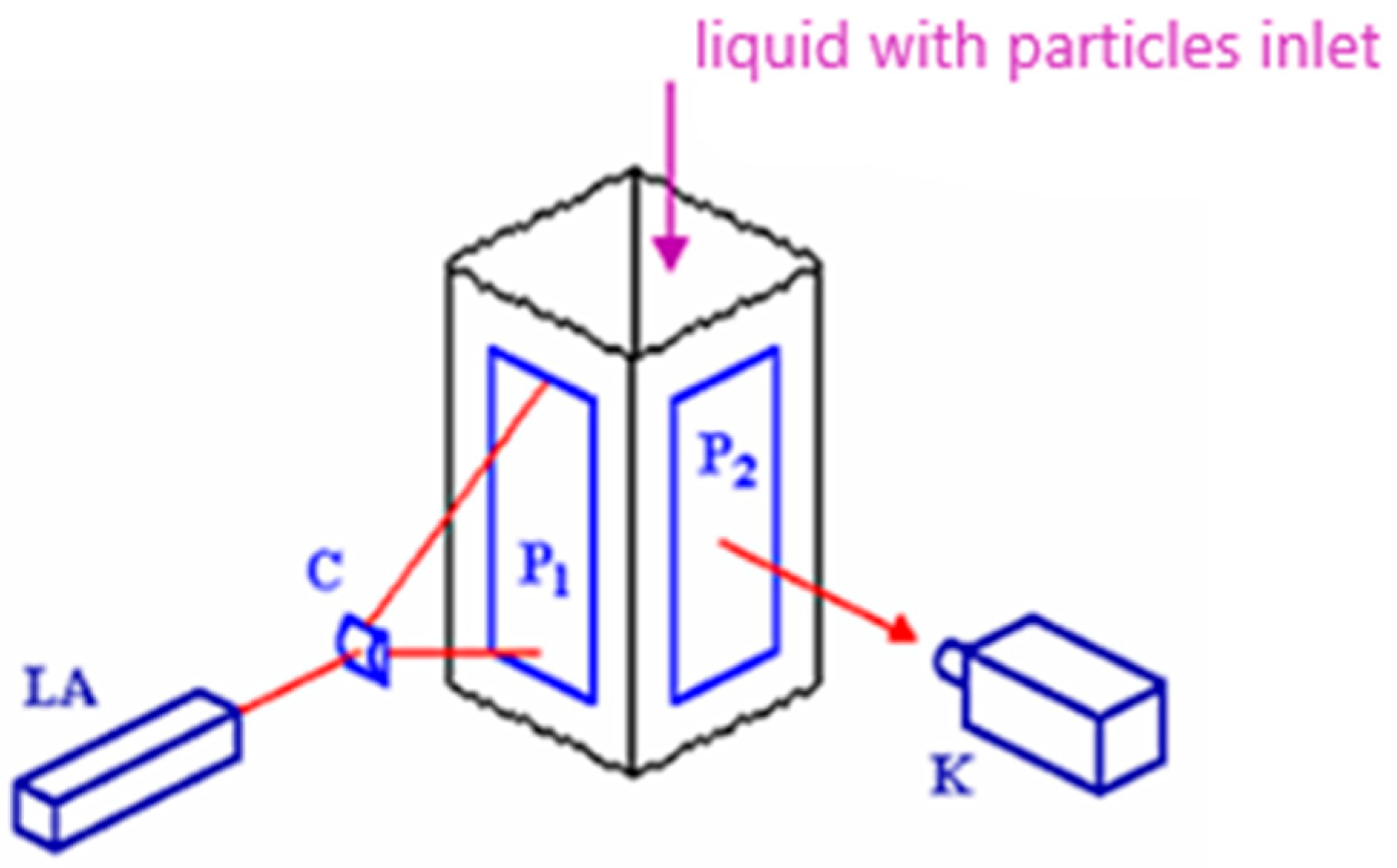
Several methods are used to investigate flow instabilities experimentally. The most suitable for comparison with numerical experiments is the PIV method. This method enables to monitor the development of vortex structures in two-dimensional cross-sectional planes. However, it is very demanding, both in the preparation of the experiment and evaluation of the measurements. To verify the mathematical model [9,22,23], an experiment was constructed to visualize Taylor vortices in the gap between concentric cylinders with a rotating inner one.

For different types of fluid and rotational speeds of the inner cylinder, the basic flow characteristics are very well-observable, including different types of vortex structures, especially in the area of emerging stable Taylor vortices. The problem of oil stability analysis has been investigated in the past and is described in sufficient detail in the literature for single-phase Newtonian fluids [15].

Vortex structures in the flow of two different immiscible liquids (oil and ethanol) of different densities and viscosities were investigated in Reference [24]. The diffusion between the fluids was very small in the case of laminar flow, and the fluids formed vortex structures separately. Their shapes corresponded to a single-phase flow at a given velocity of the inner cylinder. At higher rotational speeds, the flow was already turbulent, the liquids stirred and a mixture formed. The numerical model showed a homogeneous mixture near the walls, and a partially mixed mixture copying the vortex structures could be observed inside. The results of mathematical modeling corresponded to the experimental results.

The aim of this work is to extend the application of the single-phase mathematical model of Newtonian fluid (oil, water and ethanol) to the flow of non-Newtonian magnetorheological fluid. Experience obtained during the modeling of the oil flow [15] and water and ethanol flow [24] is the background for modeling the instability of a non-Newtonian magnetorheological fluid with a viscosity determined experimentally.

2. Experiment, Reynolds and Taylor Number

Flow visualization is a very suitable tool for experimental fluid mechanics and is necessary in the study of complex flow cases. A very interesting case is the flow structures in connection with the Taylor–Couette flow, defined by the flow of a viscous liquid in an annulus between two cylindrical surfaces that move relative to each other.

2.1. Experimental Equipment

The experimental equipment for the visualization of flow instabilities is shown in Figure 2. The base of the measuring device is a stable supporting construction with an electric motor enabling to reach the maximum speed of the inner cylinder at 2840 rpm. The electric motor is controlled by a frequency converter.

The upper part of the device consists of two concentric cylinders. The outer cylinder is made of glass, and the inner rotating cylinder is made of steel.

The parameters of the measuring area are as follows:

R1 = 65 mm	radius of the inner cylinder
R2 = 80 mm	radius of the outer cylinder
s = 15 mm	thickness of the annulus (R2 − R1)
L = 170 mm	length of the inner cylinder

The visualization [15] was realized by suitable illumination of the flowing medium with dispersed aluminum powder; see the scheme in Figure 3. The two-dimensional flow was given by an illumination unit, i.e., a light knife, which illuminates only particles in the selected section. When visualizing a three-dimensional flow, the entire space can be illuminated, but evaluation is difficult. Using visualization, the individual limit modes of Taylor vortices can be recognized, and the corresponding speed ranges can be recorded. It is also possible to observe a different number of strips that characterize the number of vortices formed.

2.2. Physical Properties of Liquids

The basic physical properties of common fluids are the density, dynamic or kinematic viscosity; surface tension and others [2,5]. The viscosity of most gases, vapors, liquids and, especially, water is governed by the so-called Newton′s law of viscosity, where the stress tensor $\stackrel{=}{\tau }\left(\mathrm{Pa}\right)$ is proportional to the velocity gradient, and dynamic viscosity is a coefficient of proportionality [25]. The fluids are called Newtonian fluids. Generalization of the Newton law of viscosity $\mu \left(\mathrm{Pa}.\mathrm{s}\right)$ is a set of nine relations:

$$\stackrel{=}{\tau }=\mu \left[\left(\nabla \overrightarrow{u}+{\left(\nabla \overrightarrow{u}\right)}^T\right)-\frac{2}{3}\left(\mathrm{div}\left(\overrightarrow{u}\right)\right)\stackrel{=}{\delta }\right],\left(Pa\right)$$

(1)

where $\nabla \overrightarrow{u}$ (s⁻¹) is a tensor of the velocity gradient with components $\left(\frac{\partial }{\partial x_i}\right)u_j\left({\mathrm{s}}^{-1}\right)$, ${\left(\nabla \overrightarrow{u}\right)}^T$ $\left({\mathrm{s}}^{-1}\right)$ is a transponse tensor of the velocity gradient with components $\left(\frac{\partial }{\partial x_j}\right)u_i$, $\mathrm{div}\left(\overrightarrow{u}\right)$ $\left({\mathrm{s}}^{-1}\right)$ is a divergence of the velocity vector and $\stackrel{=}{\delta }$ is the unit tensor. For an incompressible fluid, $\mathrm{div}\left(\overrightarrow{u}\right)=0\left({\mathrm{s}}^{-1}\right),$ and the equation has a simpler form:

$$\stackrel{=}{\tau }=\mu \left(\nabla \overrightarrow{u}+{\left(\nabla \overrightarrow{u}\right)}^T\right)=-\mu \dot{\gamma },\left(\mathrm{Pa}\right)$$

(2)

Symbol $\dot{\gamma }=\left(\nabla \overrightarrow{u}+{\left(\nabla \overrightarrow{u}\right)}^T\right)$ $\left({\mathrm{s}}^{-1}\right)$ is the strain rate tensor or the deformation rate tensor.

If the behavior of the fluids does not comply with this law, they are non-Newtonian fluids, such as suspensions, higher polymers, etc. In magnetorheological fluids, the shear stress may change depending on the direction of the magnetic field under the load, and the fluids become non-Newtonian fluids. For a non-Newtonian fluid, the analogous generalized shear stress equation applies as for Newtonian fluids, i.e., the shear stress depends nonlinearly on the velocity gradient (25). The most used empirically determined dependence is the power dependence of the viscosity on the strain rate. The most commonly used formulation is the Ostwald and de Waele (25) formulation of viscosity ${\mu }_{eff}\left(\mathrm{Pa}\mathrm{s}\right)$ in the form:

$${\mu }_{eff}=m{\dot{\gamma }}^{n-1},$$

(3)

where m and n are constants characterizing the liquid. Power functions are only interpolation functions and are not derived from a physical model of the internal structure of the fluids. For this reason, their use has been criticized, but the power functions, despite this shortcoming, capture most of the actual flow curves very well and fail only for liquids whose rheograms have inflection points. In these cases, however, it is possible to use a power function with sufficient accuracy for parts of the flow curve.

Commonly available liquids (oil, water and ethanol) were tested in the experimental equipment described above; see Figure 2. The transition state and vortex structures are best observed with hydraulic oil using aluminum powder. The viscosity of the oil with the addition of aluminum powder was measured and compared with the viscosity of the pure oil. It differed by about 2% (15). Visualization of the flow by means of aluminum powder is impossible with water, because aluminum powder is poorly dispersed in water and forms clumps, so oil and ethanol were used in the experiment. The physical properties of common liquids are given in

Table 1. Physical properties of common liquids.

	Unit	Water	Ethanol	Oil
Density	kg/m3	998	790	876
Kinematic viscosity	m2/s	1.002 × 10−6	1.5209 × 10−6	8.2182 × 10−5
Dynamic viscosity	Pa.s	0.001	0.0012	0.072

.

The physical properties of magnetorheological and ferromagnetic fluids differ from conventional Newtonian fluids, because the nanoparticles change their orientation in space when exposed to an external magnetic field. Thus, the physical properties change, and the fluids become non-Newtonian. The physical properties of magnetorheological fluids taken from the literature [2,6] are given in

Table 2. Physical properties of ferromagnetic liquids

	Unit	EMG 900	EMG 905
Concentration of nanoparticles	% vol.	17.7	7.8
Saturation magnetization	mT	99	44
Density	kg/m3	1.74∙× 103	1.2∙× 103
Dynamic viscosity	mPa.s	60	3
Melting point (at pn)	°C	−94	−94
Flash point (at pn)	°C	89	89
Initial magnetic susceptibility		18.6	3.52

.

Magnetorheological fluids EMG900 and EMG905 contain ferromagnetic particles (combination of magnetite–maghemite) with a mean particle diameter of 10 nm. The carrier liquid consists of light hydrocarbon (kerosene with additives [5]), which ensures a low viscosity. Liquids do not differ in the type of particles, only in the concentration of particles, additives and surfactants. The physical properties of the magnetorheological fluids are given in Table 2, where the viscosity is specified for a certain value of the magnetic field.

Viscosity measurements were performed for different values of the magnetic field, using a AntonPaar MCR502 (Anton Paar GmbH, Graz, Austria) rotary rheometer in a plate–plate configuration (PP20/MRD/TI). The shear loading of the liquid took place in a thin layer between two planar, circular plates [5]. A (homogeneous) magnetic field with a selectable intensity of 0–432 kA/m acted perpendicular to the direction of loading. During the experiment, the device evaluated the dependences of the shear stress in the liquid (or viscosity) on the strain rate. Samples of EMG 900 and EMG 905 fluids from Ferrotec Corp. were measured. (Ferrotec (USA) Corporation, Santa Clara, CA, USA).

Due to the strong influence of the magnetic field on the viscosity in the area of very low strain rates, the viscosity was interspersed with two different power functions in the form:

$${\mu }_{eff}=m_1{\dot{\gamma }}^{N1}+c_1{\mu }_{eff}=m_2{\dot{\gamma }}^{N2}+c_2,$$

(4)

The intersection of the viscosity curves for the area highly and less affected by the magnetic field was almost the same for different magnetic field intensities. The intersection value of the strain rate is approximately 15 s⁻¹. The result is the dependences of the shear stress and viscosity of the investigated fluids on the strain rate; see Figure 4.

Concentrated liquid EMG900 has a strong response in the area of low strain rates (most pronounced up to about 100 s⁻¹), but for high strain rates, the effect of the magnetic field is negligible, and there is even an apparent decrease in the viscosity below its basic value. Both EMG 900 and EMG 905 behave like non-Newtonian fluids under the action of a magnetic field.

2.3. Ta, a Re Number

Reynolds number Re [13, 04] is used to determine whether the fluid flow is laminar or turbulent.

$$\mathrm{Re}=\frac{\Omega R_1\left(R_2-R_1\right)}{\nu },(1)$$

(5)

where $\Omega$ (rad s⁻¹) is the angular velocity, R₁ (m) is the inner radius, R₂ (m) is the outer radius and $\nu$ (m²s⁻¹) is the kinematic viscosity. The critical value of the transition from laminar to turbulent flow is in the interval from 1100 to 1400.

Taylor number Ta [25,26] is a dimensionless quantity that characterizes the importance of centrifugal forces or so-called inertial forces due to the rotation of a fluid about an axis relative to the viscous forces.

$$\mathrm{Ta}=\mathrm{Re}\sqrt{\frac{R_2-R_1}{R_1}}=\frac{\Omega R_{1}s}{\nu }\sqrt{\frac{R_2-R_1}{R_1}},(1)$$

(6)

where s = R₂ − R₁ (m). The critical value characterizing the formation of stationary vortices is Ta_c = 41.3 (1), and the periodic wave modes of vortices occur at up to 100 times the critical Taylor number. This value differs slightly in the case of a real experiment with the finite length of the cylinder and the deformation of the vortices near the closings.

There are other, more complicated variants of these vortices (wave mode, spiral mode, etc.), where determining the critical values of the Taylor number is difficult and not unambiguous [15]. ¨The dependences of the Reynolds number (5) and Taylor number (6) on the rotational speed of the inner cylinder and the type of liquid (viscosity) were evaluated.

For magnetorheological fluids, the dependence of the Taylor number and Reynolds number on speed was solved as follows. For a given magnetic field intensity, the dependence of shear stress and viscosity on the strain rate, which was obtained experimentally [5], is known. To determine the dependence, the minimum and maximum viscosity were chosen as a constant. Subsequently, the minimum and maximum Taylor and Reynolds numbers were calculated. For viscosities within this range, it is possible to roughly estimate Ta and Re or to calculate them in the same way.

The following graphs (Figure 5) show the dependence of the Taylor number on the speed of the inner cylinder for oil, ethanol, water and magnetorheological fluid EMG 900 under the influence of the magnetic field for the maximum and minimum viscosity values; see Figure 5. From the graph, Ta = f (n), and it is evident that, for water and ethanol, it is possible to expect the formation of vortices practically at the small speed that the physical device is able to realize. For oil, Taylor vortices occur at approximately 100 rpm. From the graph, Re = f (n), and it is evident that the flow is in the laminar, transient and turbulent regime due to the possibilities of the experiment; see Figure 6. Water and ethanol flow at smaller speeds already in the turbulent mode, respectively, and transition from laminarity to turbulence. The oil flow is laminar and changes the turbulence up to speed values of the order of 1000 rpm. The magnetorheological fluid shows the initial existence of Taylor vortices even at a very low speed and high viscosity. The low viscosity liquid has properties between the test oil and the ethanol, and then, it changes into the unstable mode.

This information will be used to estimate a mathematical flow model. The graphs in Figure 5 and Figure 6 are a good orientation for numerical calculations of the flow of magnetorheological fluids between cylinders, and it should be noted that dimensionless quantities are only an indicative indicator of the transition.

3. Mathematical Model

The equations that describe the flow of real fluids are an expression of the basic physical conservation laws of mass and momentum. Physically, these laws express the balance of a quantity J (physical unit depends on the type of variable J) in a given volume [25]. According to this balance, the time change of the preserved quantity in the given volume V is equal to the flow of this quantity through the area S, which circumscribes this volume, and its production within the volume V.

$$\frac{\partial }{\partial t}{{\displaystyle \int }}_{V}JdV+{{\displaystyle \int }}_S{F}_j\left(J\right)n_{j}dS={{\displaystyle \int }}_{V}P\left(J\right)dV,$$

(7)

where J is the balanced quantity, $F_j\left(J\right)$ is the jth component of the flow density vector of the quantity J by the area dS, $n_j$ is the jth component of the normal vector and P (J) is the production density of the quantity J (production per unit time in volume V). For index j, Einstein′s summation rule is used.

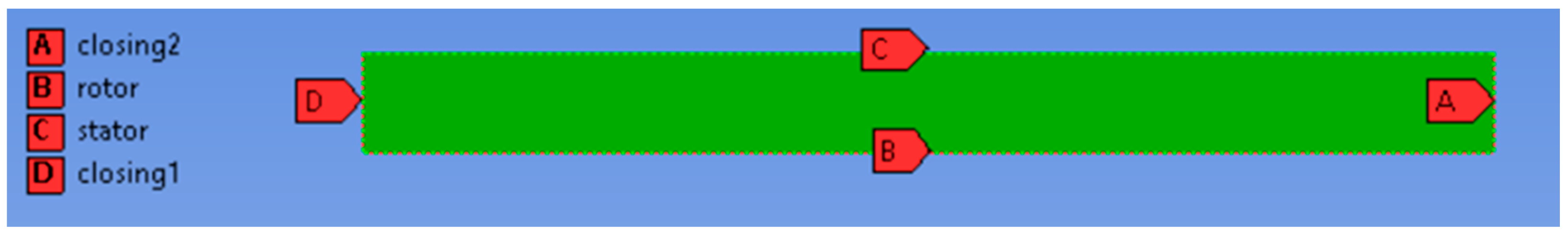
The flow of a quantity J is defined as the transfer of this quantity through a unit of area per unit time, e.g., mass flow and momentum flow. The three-dimensional model can be simplified in the case of piping systems to the two-dimensional axially symmetrical model. The defined mathematical model characterizes the flow of fluids in general spatial geometry, which is presented here by the internal space between two cylinders, where the inner one rotates. All boundary conditions on the rectangular area were of the wall type. The various rotational speeds from 10 rpm to 1000 rpm, in accordance with the physical experiment, were given on rotor, closing1 and closing2. The stator was stationary; see Figure 7. The flow was assumed as the isothermal flow, and the physical properties of the fluids are given in Table 1 and Table 2 and Figure 4.

The flow can be laminar, transient or turbulent, depending on the type of fluid and the speed of the inner cylinder. The mathematical model was applied in ANSYS Fluent software, where the laminar (DNS) model was used for the laminar flow. For transient and turbulent flow, the one-equation turbulent model Spalart–Allmaras and the two-equation SST k-ω turbulent model were used. These turbulent models are suitable for the flow of low Reynolds numbers and consider the flow in the boundary layer. In addition to molecular viscosity ${\mu }_{mol}$ (Pa.s), the turbulent viscosity ${\mu }_{turb}\left(\mathrm{Pa}.\mathrm{s}\right)$ is introduced from the general theory of turbulence. Its value at full turbulence can greatly exceed the molecular viscosity. The concept of effective viscosity ${\mu }_{eff}\left(\mathrm{Pa}.\mathrm{s}\right)$ can be introduced and is given as follows [4]:

$${\mu }_{eff}={\mu }_{mol}+{\mu }_{turb},\left(\mathrm{Pa}.\mathrm{s}\right)$$

(8)

The finite volume method was used to solve the mathematical models.

The mathematical models in MATLAB and ANSYS Fluent were solved for simplified geometries (one-dimensional and two-dimensional) and a simplified viscosity definition [27,28]. A comprehensive solution using ANSYS Fluent will be presented in Section 5.

4. Experimental Results

Hydraulic oil and ethanol were used to visualize the single-phase flow. In the experiment, the lowest speed is approximately 10 rpm, and the maximal speed is rpm 1000. The number of vortices (strips) is affected by the type of fluid and the boundary conditions. It is also used to verify the numerical experiment (0). In

Table 3. Flow visualization for a 10-rpm speed.

Speed/Liquid	Ethanol	Oil
10

, the flow results of ethanol and the oil flow for a speed of 10 rpm are shown for illustration. Further results are used in

Table 4. Speed-dependent flow simulation and comparison with the experiment.

KERRYPNX	Ethanol				Oil				EMG 900
Speed	Experiment	Swirl Velocity	Molecular Viscosity	Strain Rate	Experiment	Swirl Velocity	Molecular Viscosity	Strain Rate	Swirl Velocity	Molecular Viscosity	Strain Rate
10
50
300
700

, where they are also compared with the numerical results.

A Couette flow is very evident in the oil, and stable Taylor vortices are formed for speeds greater than 130 rpm. Ethanol shows similar properties; only the critical speed for the formation of Taylor instabilities is very small.

The following differences could be observed from the experiment due to significantly different physical properties, especially viscosity:

• Taylor vortices can be observed mainly in the area of laminar flow, so, in ethanol, they appear at a lower speed, while vortex structures in oil are formed at the speed of 130 rpm;
• the wave mode has not yet manifested;
• turbulence in ethanol causes vortex structures to be illegible;
• the experiment with the EMG 900 fluid was not performed. It was not possible to ensure the flow in the annulus and, at the same time, to influence it by means of a magnetic field acting perpendicular to the direction of load.

5. Numerical Simulation

The flow of oil, ethanol and EMG 900 was solved by the single-phase flow method. The axis of rotation was located in the vertical direction. The geometry of the area was rectangular, so rectangular elements were used. A refined mesh was created near the walls. The number of elements was 100,000. Several variants of the grid were prepared and tested using a grid convergence analysis. Physical properties were given according to Table 1. The boundary conditions were very simple; see Figure 7. The single-phase flow of oil and ethanol was solved in accordance with previous applications, i.e., laminar, turbulent model Spalart Allmaras and SST k-ω. When using the coupled differential scheme, convergence was achieved. The methodological procedure was as follows. At low rotor speeds, the calculation started with the laminar model. If the laminar model stopped converging at a higher speed, then the turbulent model was used. A comparison of the results obtained by both turbulent models was performed. Deviations of the minimum and maximum values of the pressures, velocities and shape of the stream functions were minimal.

5.1. Numerical Simulation—Oil, Ethanol and EMG 900

Verified mathematical models of single-phase Newtonian isothermal fluid were the basis for modeling magnetorheological fluid, while there is experience with the flow of individual fluids [24,27,28]. The liquids were considered as incompressible fluids, because their densities were not significantly pressure-dependent.

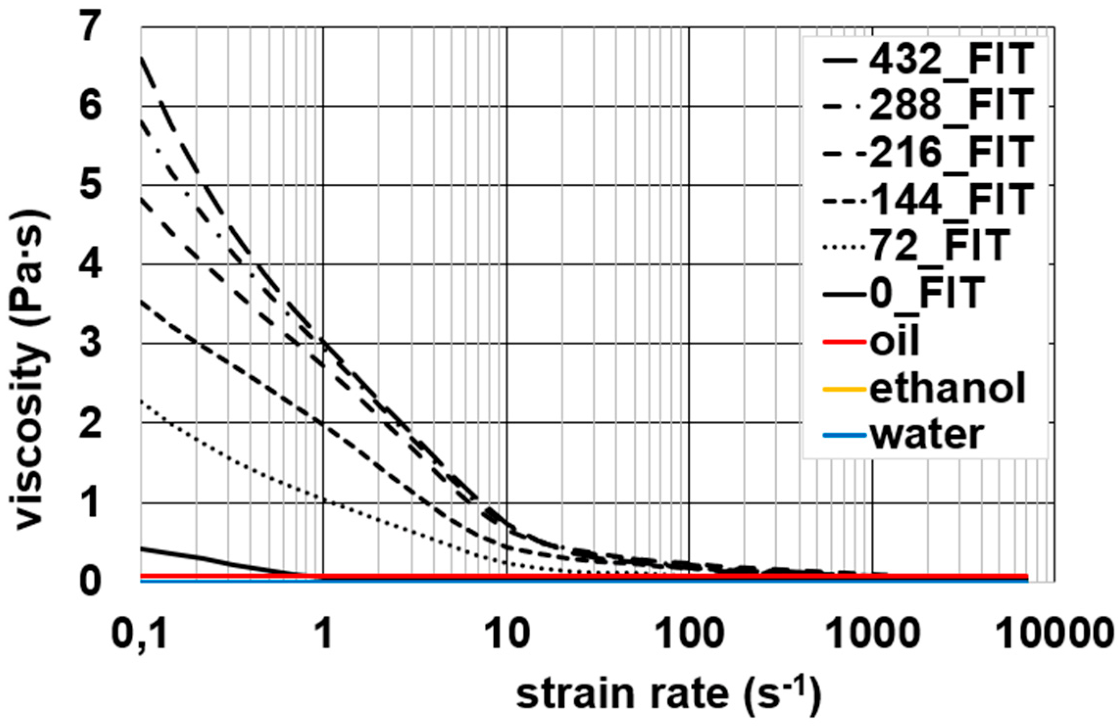
The viscosity was defined as a constant for oil and ethanol. In the case of EMG900 fluid, the viscosity was a function of the strain rate. The shape of the function was gained from experimental investigation of the physical properties of magnetorheological fluids. The functional dependence consists of two power curves according to Equation (6) and was inserted into ANSYS Fluent software. Constants $m_1,N_1,c_1,m_2,N_2,c_2$ were determined by the least squares method from the measurement of the viscosity of the EMG 900 liquid affected by the magnetic field with a selectable intensity of 0–432 kA/m and were tabulated in Reference [5]. The magnetorheological fluid was selected for the simulation under the action of a constant intensity of a mg. field of 216 kA/ m; the viscosity profile defined in ANSYS Fluent is shown in Figure 8. The horizontal axis is the strain rate and the vertical axis the viscosity. The designation of the vertical axis is related to the functional power dependence embedded in ANSYS Fluent and cannot be modified. The r numerical calculation was performed for the rotational speed in the range from 10 to 1000 rpm. Some simulations for the rotational speed of the inner cylinder were selected for graphical evaluation:

n = 10, 50, 300 and 700 rpm.

The results of the experiments and simulations for oil and ethanol and simulations for EMG 900 for selected speeds are compared in Table 4. The ethanol flow is laminar at 10 rpm; we can observe the agreement in the number of Taylor vortex strips in the experiment and the swirl velocity. At higher speeds, the flow becomes turbulent, and the strips in the experiment and simulation are less legible. The oil flow is laminar over the entire speed range. We can observe a Couette flow at 10 and 50 rpm and Taylor vortices at 300 and 700 rpm. The flow of EMG 900, according to the values of the Reynolds number, was laminar, and for higher speeds (from 300 rpm), it was switched to the turbulent mode. The flow rate shows high values of molecular viscosity for low speeds, which decrease with the increasing speed. This corresponds to a graph of the power function of the viscosity vs. strain rate. Due to the different viscosities, the number of strips is also different in oil and ethanol. The vortex structures are, of course, affected by the turbulent viscosity, and the evaluation of the laminar, turbulent and effective viscosity will be made in

Table 5. Mean values of the viscosity mol., turb., eff. and strain rate.

Speed		(rpm)	10	50	300	700
oil	oil viscosity mol.	(Pa.s)	0.0726	0.0726	0.0726	0.0726
	oil viscosity turb.	(Pa.s)	_	_	_	_
	oil viscosity eff.	(Pa.s)	_	_	_	_
	oil strain rate	(s−1)	5.27	26.47	205.99	519.31
ethanol	ethanol viscosity mol.	(Pa.s)	0.00120	0.00120	0.00120	0.00120
	ethanol viscosity turb.	(Pa.s)	_	0.00416	0.03361	0.07512
	ethanol viscosity eff.	(Pa.s)	_	0.00536	0.03481	0.07632
	ethanol strain rate	(s−1)	7.13	59.40	315.88	682.16
EMG	EMG viscosity mol.	(Pa.s)	1.35660	0.48630	0.14999	0.12029
	EMG viscosity turb.	(Pa.s)	_	_	0.00110	0.01843
	EMG viscosity eff.	(Pa.s)	_	_	0.15816	0.13872
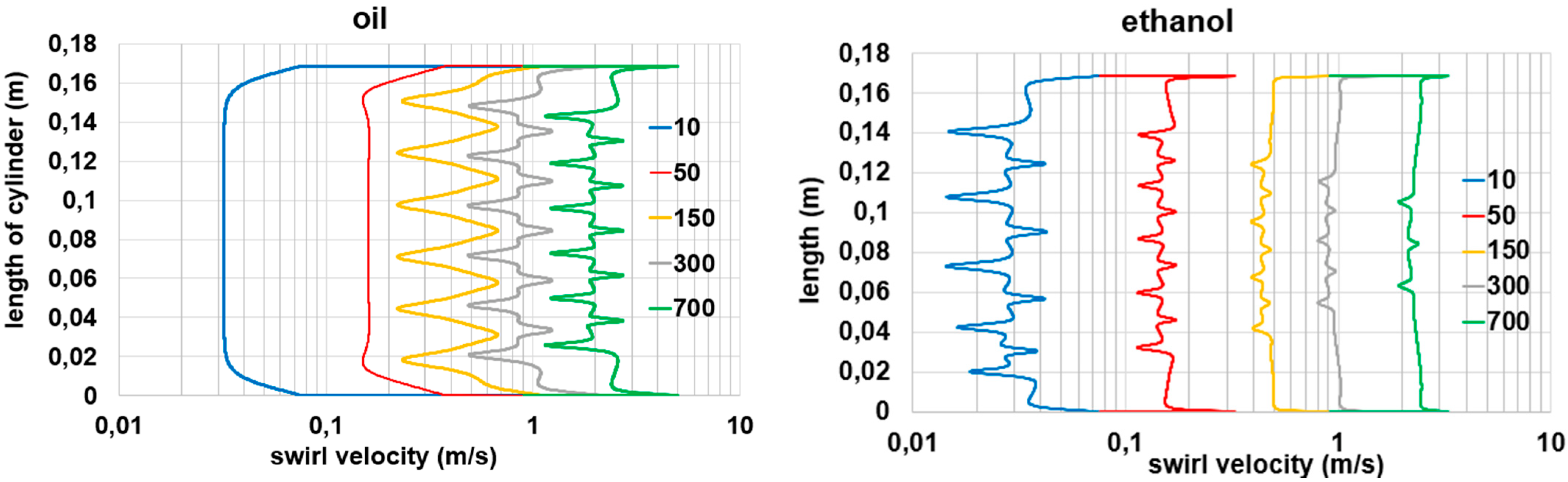
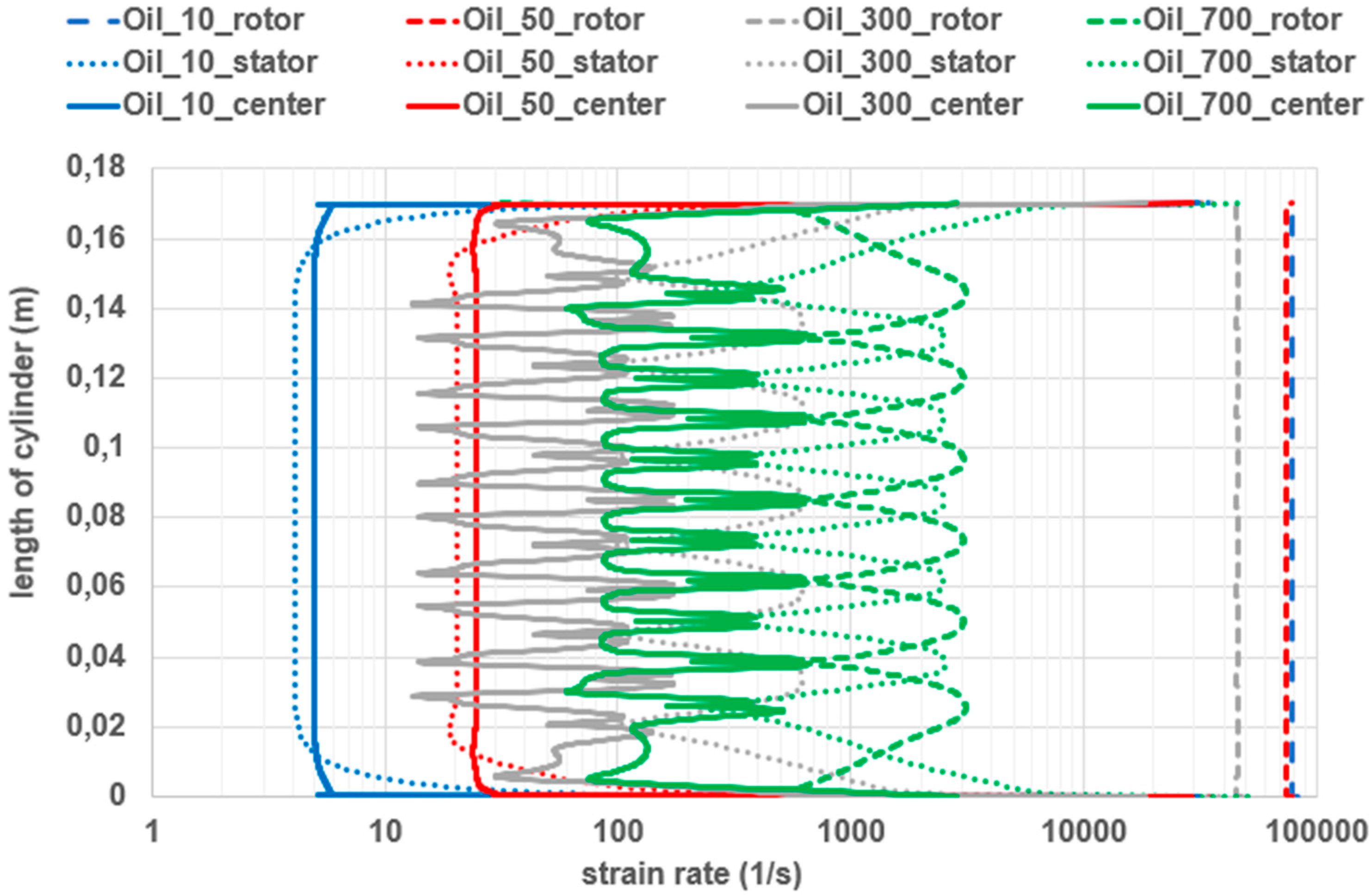
	EMG strain rate	(s−1)	5.21	25.94	363.47	882.62

. To compare the results, it appears that the most illustrative is the presentation of the swirl velocity in the logarithmic coordinates. Then, the vortex structures were recognizable even at lower values. The advantage of numerical simulation is the possibility of evaluating the strain rate, which, for a given geometry and properties of the fluid, cannot be determined analytically and which is, of course, used to determine the viscosity. The strain rate also copied the vortex structures and is displayed in the same range of values for comparison:

• swirl velocity in logarithmic coordinates <0.001; 5>
• molecular viscosity <0; 1.4>
• strain rate in logarithmic coordinates <1; 100,000>

It can be seen from Table 4 that the vortex structures of the swirl velocity for oil and ethanol coincide with the experiment.

Figure 9 evaluates the swirl velocity profile in the logarithmic coordinates depending on the liquid (oil or ethanol) and the speed of the rotor in the middle of the gap. The number of strips in the experiment can be determined by the number of peaks.

Periodic changes along the length of the cylinder copy all the other variables, such as the pressure, strain rate, etc.; see Figure 10.

5.2. Evaluation of Viscosity of Non-Newtonian Fluid EMG 900

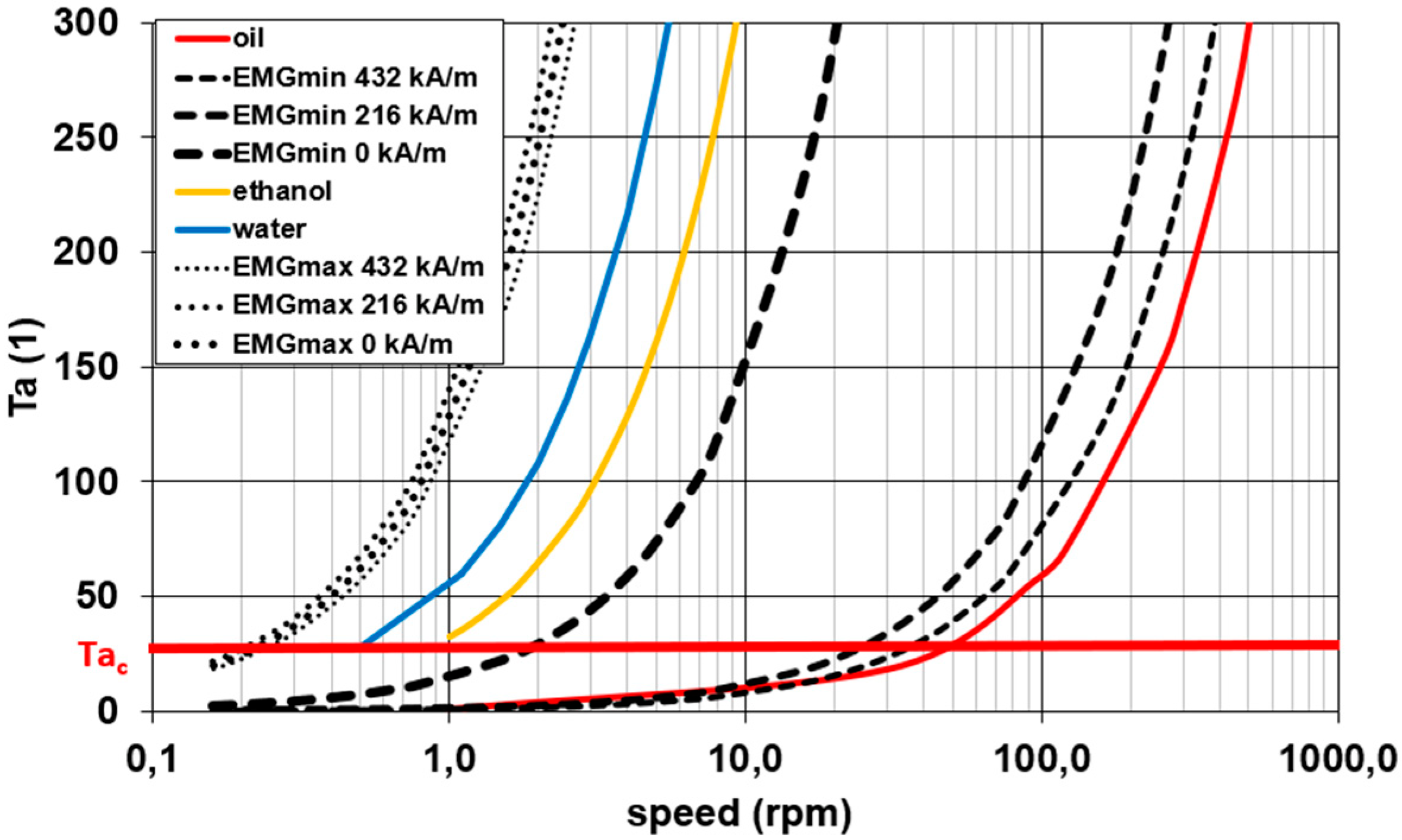
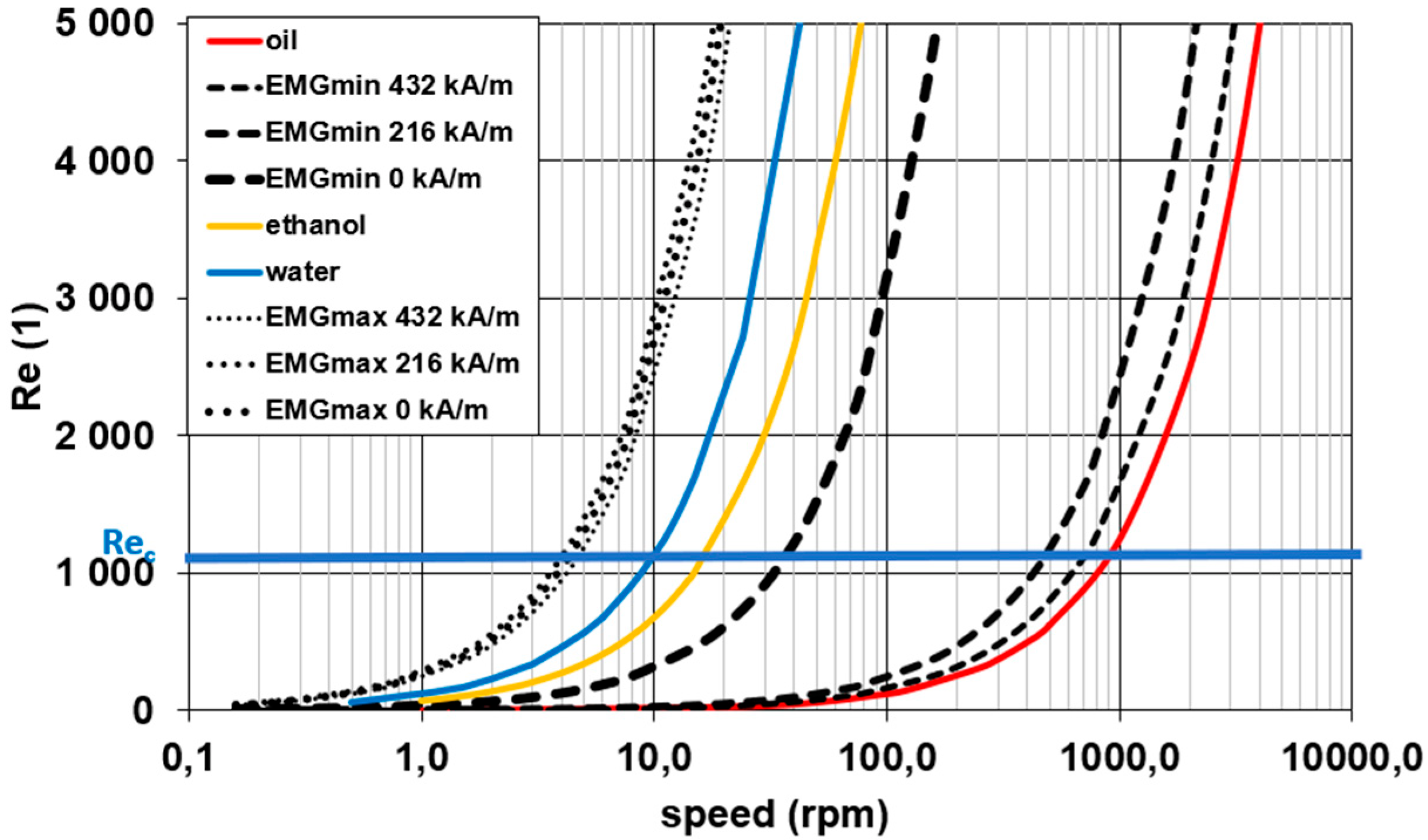
Estimation of the flow type of Newtonian fluids is possible for simple geometries based on the evaluation of the Reynolds number; see Figure 6. Estimation of the flow type for non-Newtonian fluids is problematic, because the molecular viscosity varies depending on the flow. In Figure 6, only the maximum and minimum molecular viscosity values are used. However, the viscosity values for flow in the real region are different at each point. Based on the values of the average molecular and turbulent viscosity, we can estimate the average degree of turbulence for the flow of non-Newtonian fluids

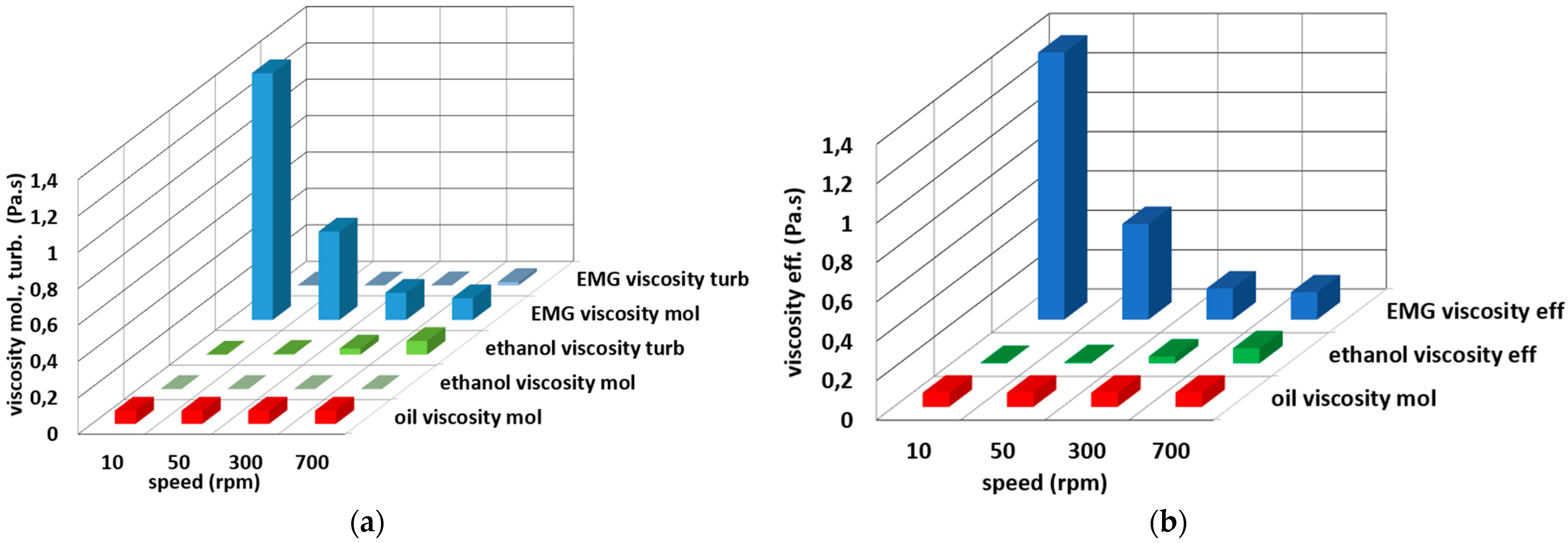
An important result of the simulation is the molecular, turbulent and effective viscosities (sum of the laminar and turbulent viscosities) according to the type of flow and strain rate. Viscosity can be evaluated using isolines in a given area. Due to further use, it is important to evaluate the mean values of the molecular, turbulent and effective viscosities and the strain rate within the fluid; see Table 5, where

• laminar flow: values of the molecular viscosity and strain rate are written in black;
• turbulent flow: values of the molecular, turbulent and effective viscosities and strain rate are written in red.

At a very low turbulence, it can be observed that the effective viscosity differs very little from the molecular viscosity. With increasing the speed, it changes to a more pronounced turbulent mode; the value of the turbulent viscosity documents the degree of turbulence and, along with the effective viscosity, increases significantly. The strain rate increases with the speed and, more significantly, with the laminar flow.

For comparison, the average values of the molecular, turbulent and effective viscosities for the above speed variants are evaluated; see Figure 11. It can be seen that the turbulent viscosity is most significant for ethanol, so the degree of turbulence of the ethanol flow is high. The turbulent viscosity does not exist for oil that flowed in the laminar mode.

The EMG 900 fluid flow is turbulent at speeds higher than 30 rpm and is more complicated. The so-called molecular viscosity is a power function of the strain rate, and it is high for low speed and decreases with the increasing rotational speed. The numerical calculation starts from the initial approximation of all the variables. The velocity profile, effective viscosity and all the other variables are adjusted in the iteration process based on the solution of a turbulent mathematical model. This also adjusts the value of the so-called molecular viscosity and, consequently, the turbulent viscosity, which is almost equal to zero. The effective viscosity (sum of the turbulent and molecular viscosities) is only slightly higher than the molecular viscosity. The flow is slightly turbulent, which can be seen in the graphical representation of the contours in Table 4.

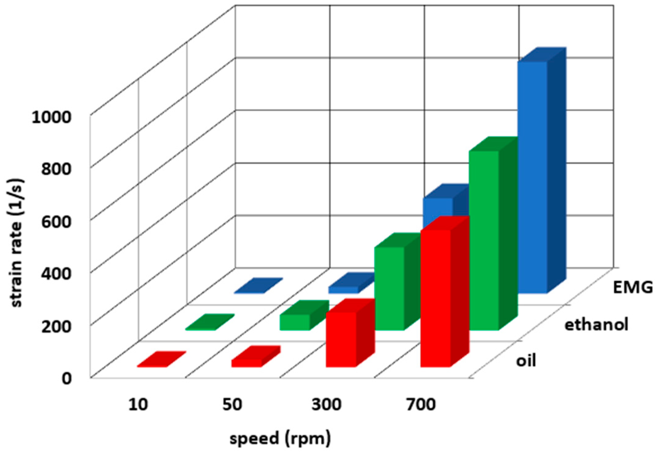
The strain rate increases for all the fluid variants; see Figure 12.

6. Discussion

The aim of the work was to investigate the occurrence of Taylor vortices in the gap between two cylinders, where the inner cylinder rotates. Single-phase Newtonian and non-Newtonian magnetorheological fluids were investigated.

The first part was devoted to the instabilities of a mathematical model for the Newtonian fluid flow of oil and ethanol and implementation into ANSYS Fluent software. The mathematical models were verified experimentally.

• single-phase flow and the formation of vortex structures (Taylor vortices) can be characterized by Taylor and Reynolds numbers;
• The mathematical model was as follows:

  −

  oil—laminar flow model;

  −

  ethanol—for speeds of 10 and 30 rpm, a model of laminar flow was used; for higher speeds, the model was turbulent.

The simulated results agreed with the experiment and confirmed the suitability of the tested mathematical models. This experience was used to model a ferromagnetic or magnetorheological fluid.

The aim of the second part of the work was to verify how the single-phase ferrofluid EMG 900 behaved when flowing in the annulus, where the inner cylinder rotated and exerted a magnetic field.

• The flow of magnetorheological fluid was characterized by the Taylor and Reynolds numbers, depending on the shear stress, respectively, the viscosity and intensity of the magnetorheological field. An analytical evaluation of the Taylor and Reynolds numbers was difficult, so these values were determined for the minimum and maximum viscosity values at a given intensity in the magnetorheological field. For given speeds and electromagnetic field values, it was possible to estimate whether the flow was laminar or turbulent and, in addition, whether Taylor vortices would appear.
• The strain rate and viscosity were not constant within the range; the mean values of these quantities could be determined.
• The mathematical model was as follows:

  −

  EMG 900—if the speeds were 10 and 30 rpm, the mathematical model used was laminar; for higher speeds, it was turbulent.

The results of the research confirmed the suitability of the used mathematical models implemented in computer software ANSYS Fluent. The experience in modeling the flow of oil and ethanol in the annulus during the rotation of the inner wall was used to model the flow of the EMG 900 fluid. The type of mathematical model was determined roughly from the graphs Ta and Re. More precisely, the problem was solved numerically as laminar and turbulent, respectively, and the values of the molecular and effective viscosities were compared.

References

1. Blums, E.; Cebers, A.; Maiorov, M. Magnetic Fluids; Walter de Gruyter: Berlin, Germany; New York, NY, USA, 1997; 416p, ISBN 3-11-014390-0. DM 378. [Google Scholar]
2. Odenbach, S. Ferrofluids Lecture Notes in Physics; Springer: Berlin/Heidelberg, Germany. Available online: http:/www.springer.de/phys/ (accessed on 26 November 2002).
3. Fialová, S.; Kozubková, M.; Jablonská, J.; Havlásek, M.; Pochylý, F.; Šedivý, D. Journal bearing with non-Newtonian fluid in the area of Taylor vortices. IOP Conf. Ser. Earth Environ. Sci. 2019, 240, 062013. [Google Scholar] [CrossRef]
4. ANSYS Fluent Theory Guide; ANSYS Inc: Canonsburg, PA, USA, 2019.
5. Experimental Measurement of the Viscous Reply of the Ferrofluids in Magnetic Field; Grant Agency Project: GA101/19-06666S; Internal Research Report; Grant Agency of Czech Republic: Ostrava, Czech Republic, 2020.
6. Odenbach, S.; Thurrn, S. Magnetoviscous Eflects in Ferrofluids. Technical Report; Springer: Heidelberg, Germany, 2002; ISBN 354-0430687. [Google Scholar]
7. Guru, B.S.; Hiziroglu, H.R. Electromagnetic Field Theory Fundamentals; Cambridge University Press: Cambridge MA, USA, 2004; ISBN 0-521-830168. [Google Scholar]
8. Chari, M.V.K.; Salon, S.J. Numerical Methods in Electromagnetism; Academic Press: San Diego, CA, USA; London, UK, 2000; ISBN 0-12-615760-X. [Google Scholar]
9. Jiles, D. Introduction to Magnetism and Magnetic Materials; CRC Press: New York, NY, USA, 2016. [Google Scholar]
10. Lenci, A.; Chiapponi, L. An Experimental Setup to Investigate Non-Newtonian Fluid Flow in Variable Aperture Channels. Water 2020, 12, 1284. [Google Scholar] [CrossRef]
11. Tong, T.A.; Yu, M.; Ozbayoglu, E.; Takach, N. Numerical simulation of non-Newtonian fluid flow in partially blocked eccentric annuli. J. Pet. Sci. Eng. 2020, 193, 107368. [Google Scholar] [CrossRef]
12. Lacassagne, T.; Cagney, N.; Balabani, S. Shear-thinning mediation of elasto-inertial Taylor–Couette flow. J. Fluid Mech. 2021, 915, A91. [Google Scholar] [CrossRef]
13. Kaushik, V.; Wu, S.; Jang, H.; Kang, J.; Kim, K.; Suk, J.W. Scalable Exfoliation of Bulk MoS2 to Single- and Few-Layers Using Toroidal Taylor Vortices. Nanomaterials 2018, 8, 587. [Google Scholar] [CrossRef] [PubMed] [Green Version]
14. Davey, A. The growth of Taylor vortices in flow between rotating cylinders, 1962. J. Fluid Mech. 1962, 14, 336–368. [Google Scholar] [CrossRef]
15. Farník, J. Investigation of the Instabilities in between Two Rotating Coaxial Cylinders. Ph.D. Thesis, VSB-TU Ostrava, Czech Republic, 2006. [Google Scholar]
16. Altmeyer, S.; Do, Y.; Lai, Y.-C. Dynamics of ferrofluidic flow in the Taylor-Couette system with a small aspect ratio. Sci. Rep. 2017, 7, 40012. [Google Scholar] [CrossRef] [PubMed] [Green Version]
17. Dong, S. Direct numerical simulation of turbulent Taylor–Couette flow. J. Fluid Mech. 2007, 587, 373–393. [Google Scholar] [CrossRef] [Green Version]
18. Teng, H.; Liu, N.; Lu, X.; Khomami, B. Direct numerical simulation of Taylor-Couette flow subjected to a radial temperature gradient. Phys. Fluids 2015, 27, 125101. [Google Scholar] [CrossRef]
19. Maksimov, F.A. Numerical Simulation of Taylor Vortex Flows Under the Periodicity Conditions. In Applied Mathematics and Computational Mechanics for Smart Applications. Smart Innovation, Systems and Technologies; Jain, L.C., Favorskaya, M.N., Nikitin, I.S., Reviznikov, D.L., Eds.; Springer: Singapore, 2021; Volume 217. [Google Scholar] [CrossRef]
20. Wang, H. Experimental and Numerical Study of Taylor-Couette Flow. PhD Theses, Iowa State University, Ames, IA, USA, 2015; p. 14462. [Google Scholar] [CrossRef]
21. Baek, S.I.; Ahn, J. Large Eddy Simulation of Film Cooling Involving Compound Angle Holes: Comparative Study of LES and RANS. Processes 2021, 9, 198. [Google Scholar] [CrossRef]
22. Fialová, S.; Pochylý, F.; Volkov, A.V.; Ryzhenkov, A.V.; Druzhinin, A.A. The Mathematical Model Simplification Methods for Caculating Flows in the Hydraulic Turbines Flow Path. Teploenergetika 2021, 12, 1–11. (In Russian) [Google Scholar]
23. Pochylý, F.; Fialová, S.; Krausová, H. Variants of Navier-Stokes Equations. In Engineering Mechanics 2012; Book of Extended Abstracts; AV CR: Prague, Czech Republic, 2012; pp. 1011–1016. ISBN 978-80-86246-40-6. [Google Scholar]
24. Kozubková, M.; Jablonská, J.; Bojko, M.; Pochylý, F.; Fialová, S. Multiphase Flow in the Gap between Two Rotating Cylinders. MATEC Web Conf. 2020, 328, 02017. [Google Scholar] [CrossRef]
25. Bird, R.B.; Stewart, W.E.; Lightfoot, E.N. Transport Phenomena; John Wiley & Sons: Hoboken, NJ, USA, 2002; ISBN 0-471-41077-2. [Google Scholar]
26. Fialová, S.; Pochylý, F.; Malenovský, E. Numerical analysis and simulations of the magnetic field and hydrophobicity effect on the journal bearing dynamics. Proc. Inst. Mech. Eng. Part J J. Eng. Tribol. 2017, 231, 561–571. [Google Scholar] [CrossRef]
27. Šedivý, D.; Ferfecki, P.; Fialová, S. Influence of Eccentricity and Angular Velocity on Force Effects on Rotor of Magnetorheological Damper. EPJ Web Conf. 2018, 180, 555–559. [Google Scholar]
28. Tuma, J.; Kozubkova, M.; Pawlenka, M.; Mahdal, M.; Simek, J. Theoretical and Experimental Analysis of the Bearing Journal Motion Due to Fluid Force Caused by the Oil Film. MM Sci. J. 2018, 2018, 2466–2472. [Google Scholar] [CrossRef]
Figure 1. Vortex structures between two concentric cylinders.
Processes 09 01832 g001
Figure 2. Flow between concentric cylinders during rotation of the inner cylinder, experiment and photos of the Couette and Taylor flow [15].
Processes 09 01832 g002
Figure 3. Flow visualization scheme (LA—laser, C—cylindrical lens creating a light knife, K—camera and P1 and P2—windows).
Processes 09 01832 g003
Figure 4. Viscosity dependence on the strain rate for oil, ethanol, water and EMG 900 [5].
Processes 09 01832 g004
Figure 5. Taylor number vs. speed for oil, ethanol, water and EMG 900 (Tac = 41).
Processes 09 01832 g005
Figure 6. Reynolds number vs. speed for oil, ethanol, water and EMG 900 (Rec = 1100 to 1300).
Processes 09 01832 g006
Figure 7. Axisymmetric region and boundary conditions.
Processes 09 01832 g007
Figure 8. Dependence of viscosity on the strain rate and detail in ANSYS Fluent.
Processes 09 01832 g008
Figure 9. Dependence of the swirl velocity in logarithmic coordinates on cylinder length.
Processes 09 01832 g009
Figure 10. Dependence of the strain rate in logarithmic coordinates on the length of the cylinder for oil on the rotor, stator and in the middle of the gap.
Processes 09 01832 g010
Figure 11. Computed mean viscosities: molecular, turbulent and effective.
Processes 09 01832 g011
Figure 12. Mean strain rate for different variants of the numerical calculations.
Processes 09 01832 g012