Article

Voltage Stability Index Using New Single-Port Equivalent Based on Component Peculiarity and Sensitivity Persistence

1
School of Electronics and Information Engineering, Wuxi University, Wuxi 214105, China
2
School of International Education, Wuxi University, Wuxi 214105, China
3
Department of Management, Faculty of Management in Production and Transportation, Politehnica University of Timisoara, 300191 Timisoara, Romania
4
College of Physics and Electronic Information Engineering, Neijiang Normal University, Neijiang 641100, China
5
School of Electrical Engineering, Chongqing University, Chongqing 400044, China
6
Faculty of Automation, Huaiyin Institute of Technology, Huai’an 223003, China
*
Authors to whom correspondence should be addressed.
Submission received: 14 September 2021 / Revised: 11 October 2021 / Accepted: 15 October 2021 / Published: 18 October 2021
(This article belongs to the Special Issue Clean Energy Conversion Processes)

Abstract

:
A voltage stability index is proposed using a new single-port equivalent depending on component peculiarity representation and sensitivity persistence to locate and determine long-term voltage instability in transmission and distribution power networks. The suggested single-port equivalent effectively represents the equivalence of various component types and assures the consistency of sensitivity information before and after the equivalence which is compulsory for the equivalent accuracy in estimating the voltage stability analysis. The stability index is derived from the new single-port equivalent to determine the system voltage instability. The proposed stability index is compared with indices based on virtual impedance and Thevenin impedance models. This new stability index shows more accuracy and effectiveness as compared to the indices based on virtual and Thevenin equivalent models. The index also determines the weak buses, where an improvement or functional measure can be used to reduce the system voltage instability. The validity of the proposed equivalent approach and stability index is presented by utilizing two radial systems, four IEEE systems and an actual system having bus size from five to 1010 buses.

1. Introduction

Voltage instability has become a major concern for the power sector as many major blackouts, and voltage collapses have occurred across the world in recent years [1,2,3]. The IEEE and CIGRE had collaborated on power system stability concerns and established various ideas and terminologies for voltage instability issues [4]. The primary purpose of this study is to evaluate and analyze the longer-term voltage stability problems. In the literature, a wide range of stability indices are developed to assess the longer-term voltage stability of the power network and highlight the critical buses [5,6,7,8]. The indexes evaluating the stability of the power system are commonly classified as system indexes and local indexes.
The system indexes which utilize the continuation power flow (CPF) [9,10] and optimization techniques [11], e.g., system load margin, do not require network equivalence and can accurately assess the voltage instability and the stability margin of the power system. Furthermore, the system indices are unable to detect susceptible locations in the system which are responsible for the voltage instability. To evaluate the instability of system voltage, local bus-based indices have been suggested, and these indices utilize local bus-based equivalent systems to identify vulnerable buses [12,13,14]. However, the currently established local equivalent systems lack the characteristics of various elements in equivalence and the persistence of sensitivity information before and after the equivalent. Generators, loads, line branches, transformer branches, and grounding branches all operate differently in power networks and, therefore, the equivalent network must be particularly interpreted. The existing equivalent approaches do not consider the variations in equivalence between these system components, resulting in equivalence inaccuracy and the inability to guarantee sensitivity persistence before and after equivalence. The lack of characteristics of system components and persistence of sensitivity information within the local equivalent create inconsistencies in local indicators which can also produce imprecise estimations of voltage stability.
Thevenin equivalent local bus-based indicators estimating voltage instability are widely researched and received great attention [15,16,17,18,19,20]. Although, the evaluation of equivalent parameters in Thevenin equivalent is predicated on the assumption that the parameters remain constant in various states of the system. As a result, determining the equivalent parameters for Thevenin, which characterize the complete system outside of the location of concern can be inaccurate [21,22]. Therefore, it is essential to ensure the sensitivity persistence for the variables before and after the equivalence calculation. Some enhancements can be observed in [23,24,25], wherein just a single system state is needed, or the equivalent impedance and voltage are shown to be load-independent. However, both Thevenin and the improved method [23,24,25] lack the effective representation of system components and also lack sensitivity persistence. So, determining an effective local equivalent network to represent system components better and fulfil the persistence of sensitivity has become an important concern for local indicators [12,15].
To improve accuracy in estimating the voltage stability, an index using a new single-port equivalent depending on component peculiarity representation and sensitivity persistence is presented in this paper to calculate the voltage instability for the longer term. Some of the significant improvements are mentioned below:
i.
The voltage stability index is calculated utilizing a novel single-port equivalent based on component peculiarity representation and sensitivity persistence which utilizes the characteristics of just a single system state. The distinct component types addressed by the suggested equivalent are line branches, generators, transformer branches, loads, and grounding branches. Before and after the equivalency, the sensitivity relationship for the bus under investigation is held constant.
ii.
The index based on the new single-port equivalent estimates the highest load capacity for every load bus that can be utilized to determine the voltage stability of the system and the positions of weak buses. The knowledge about weak buses can help design and manage practices to limit voltage instability.
The following is a breakdown of the organization of the paper. Section 2 introduces the new single-port static equivalent. In Section 3, the derived index depending on new network equivalency for locating and determining voltage instability is demonstrated. Section 4 shows the simulation findings, and, finally, the conclusion is presented in Section 5.

2. New Single-Port Equivalent Depending on Component Peculiarity and Sensitivity Persistence

The main focus is to develop an efficient and accurate equivalent network that represents the components of the equivalent system outside of each individual load bus quite effectively and is, therefore, consistent in sensitivity information. Then, the index is derived using a new network equivalent to the estimated maximum load-ability for voltage stability margin for every single load bus. After that, the equivalence method can be incorporated in any load bus in a distribution or transmission system.
The suggested general equivalent network for each bus j in the given system is shown in Figure 1.
There are totally two buses, namely bus “i” and “j” in the suggested equivalent network as shown above in Figure 1, generally i is called virtual equivalent generator bus, and j is known as load bus. The proposed general equivalent network usually consists of the four (04) equivalent system component types given below:
(1)
yeqij is named as admittance value of equivalent branches in between load bus j and virtual generator bus i signifying the equivalent to line or transformer type branches of the whole network outside of load bus j;
(2)
Eeqij is called the voltage value of bus i signifying the equivalent of all generators located outside of j;
(3)
ILeqj is the current injected into equivalent load bus j, signifying the equivalence of all loads of the whole outside network of j;
(4)
yeqb0i is the admittance rate for the grounding branches connected with j, signifying the equivalent of all respective branches of the whole outside network relative to j.
The fundamental equations for the original bus voltage system ahead of the equivalence can be so formulated in a separate arrangement of generator and load buses, such as:
Y G G Y G L Y L G Y L L E G V L = I G I L
where, the sub-script G is used to represent generator buses. Furthermore, the sub-script L signifies load buses. EG stands for the voltage vectors signifying the given generator buses, whereas VL stands for voltage vectors signifying the given load buses. IG stands for injected current vectors of generator buses whereas, IL stands for injected current vectors of load buses. YGG, YLG, YGL, and YLL represent the corresponding sub-matrices of the bus admittance matrix Y before the equivalence. From Equation (1), we can write
I G = Y G G E G + Y G L V L
I L = Y L G E G + Y L L V L
Using Gaussian elimination method [26], we can take value of EG from Equation (2) and after putting value of EG in Equation (3) we get,
( Y L L Y G L Y G G 1 Y L G ) V L = I L Y L G Y G G 1 I G
So, by using the Gaussian elimination method to eliminate the whole network nodes outside of bus under consideration in Equation (1), we can get the self-admittance of the non-generator coupled node as mentioned below,
Y L L E Q = Y L L Y L G Y G G 1 Y G L
Similarly, using the Gaussian elimination method to eliminate the whole outside network nodes (virtual generator node) in the single port equivalent network of Figure 1 we can get the self-admittance of the non-generator node as given below,
Y L L E Q = Y L L Y L G Y G G 1 Y G L
Apex represent the corresponding equivalent quantity after equivalence. The equivalent network shown in Figure 1 comprises of an only non-generator node or load node j and virtual generator node i, therefore, we have Y L G = Y G L = y e q i j Y G G = y e q i j , and Equation (6) can be written as follows,
Y L L E Q = Y L L y e q i j
The result should be the same before and after the equivalence, that means the self-admittance of the non-generator coupled node should be same, so we can get the following Equation (8) by combining Equations (5) and (7),
y e q i j = Y L L Y L L + Y L G Y G G 1 Y G L
Depending on the persistence of the sensitivity relationship [27], we can get the self-admittance of the non-generator coupled node after equivalence as follows,
Y L L = Y L L Y L L j i Y L L i i 1 Y L L i j
YLL, is the non-generator node admittance matrix before equivalence, YLL(x)(y) is the sub-matrix of YLL, x and y can be i and j. Putting value of Equation (9) into Equation (8) then we get,
y e q i j = Y L G Y G G 1 Y G L Y L L j i Y L L i i 1 Y L L i j
After obtaining the equivalent branch admittance yeqij, we can get the equivalent grounding branch admittance yeq0ij using self-admittance of the non-generator coupled node after equivalence minus the sum of other branch admittance connected with the non-generator coupled node j, as given
y e q 0 i j = Y L L y e q i j y L
We can get Y L L , the self-admittance of the non-generator coupled node after equivalence from Equation (9) and equivalent branch admittance yeqij from Equation (10), i.e., is the sum of branch admittance connected with the non-generator coupled node j except the equivalent branch and equivalent grounding branch.
Depending on power flow and persistence of the sensitivity relationship [27] we can get the equivalent load injection current ILeqj and the equivalent virtual generator voltage Eeqij as follows:
I L e q j = I L Y L L j i Y L L i i 1 I L i
E e q i j = Y L G j ( e q i j ) 1 ( Y L G j i Y L L j i Y L L i i 1 Y L G i i ) E G i
ILi and EGi are vectors of the non-generator node injection current and the voltage of the generator node in the external network before equivalence, respectively.
YLG is the sub-matrix used for admittance of non-generator node, as well as the generator node before equivalence, YLG(x)(y) is the sub-matrix of YLG, where x and y can be i and j. YLGj(eqij) is named as the node admittance matrix relevant to the non-generator coupled node j and the equivalent virtual generator node after equivalent.
From Figure 1, so the Eeqij in Equation (13) can be simplified as given below
E e q i j = 1 y e q i j [ Y L G j ( e q i j ) 1 ( Y L G j i Y L L j i Y L L i i 1 Y L G i i ) E G i ]
The procedure of new single-port equivalent methodology depending on the component peculiarity representation as well as sensitivity persistence proposed in this paper is demonstrated in the following lines.

2.1. Data Preparation

We can get the following information based on the power flow before equivalence, the node admittance sub-matrices, namely, YGG, YGL, YLG, YLLji, YLLij, YLLii, YLGji, YLGii, the generator node voltage EGi of the external network, self-admittance of load node YLL, the load node voltage VL and load node injection current IL.

2.2. Calculating Equivalence Parameters

Based on the data extracted from the above procedure, we can obtain the equivalent branch admittance yeqij, equivalent grounding branch admittance yeqb0i, equivalent load injection current ILeqj and virtual generator voltage Eeqij from Equations (10)–(12) and (14). We can calculate the complex power output of the virtual generator node as follows,
S e q i j = E e q i j y e q i j E e q i j V L
‘*’ indicates the complex conjugate.
With all equivalent parameters yeqij, yeqb0i, ILeqj, and Eeqij the single-port equivalence model portrayed in Figure 1, is now established.

2.3. Features of Proposed Model of Equivalent

The proposed single-port model has several advantages. Such as:
(a)
Sensitivity Persistence: The main advantage of the proposed model lies in the fact that it maintains the persistence in (i) non-generator voltage (node) w.r.t. generator voltage (node) and (ii) non-generator voltage (node) w.r.t. non-generator current (injected). The existing methods available in literature do not necessarily represent the sensitivities equivalence between the given variables. Furthermore, in the power system analysis, it is mandatory to model the variations of variables. Therefore, maintaining the persistence of sensitivities is extremely significant for the mandatory accuracy for better estimation of voltage instability.
(b)
Component Peculiarity Representation: Another important aspect of this model lays in the fact that it consists of four component types, namely: equivalent generators, equivalent branches, equivalent grounding branches and equivalent loads given in (12) and (13). It shows that Eeqij is only relevant to the node’s admittance and the generator voltages of the whole outside system respective to the under study bus. In contrast, ILeqj is only relevant to the matrix for node admittance, as well as the load outside the bus in discussion. Compared to the existing local equivalent, such significations effectively comprehend the effects of equivalence for different components, which is important for stability analysis. In (10) and (11), one can see that only relation of equivalent impedances goes to the network impedances, which further extend to the topology of the given system. It is pertinent to mention that it is independent of injected currents, voltages, and loads. As of (14), the voltage equivalent is linked with the topology of system and network impedance and the generator voltage; however, it is fully independent of current (injected) and loads. The features mentioned above are necessary for the establishment of the bus-based stability index voltage.
(c)
Finally, this model is highly suitable for all types of load buses in transmission and distribution networks, such as parallel, radial, and looped buses. The parameters involved in the equivalent network are estimated using the information provided by one single state of the system. These features ensure the high accuracy ratio when this model is incorporated to calculate voltage stability.

3. Derivation of Voltage Stability Index Based on New Single-Port Equivalent

The maximum loading parameter λmaxj for each load bus j or selected critical load bus j are calculated using the following derived index based on bus loading level. Figure 1 shows the general equivalent network for any load bus j. Using power balance equation for equivalent network shown in Figure 1, we obtain the following equation:
S L e q j S L j = [ ( V j V i ) y e q i j + V j y e q 0 i j ] V j
where SLj is the actual complex load power on bus j and we can also write Equation (16) in terms of voltage as follows:
I L j Z e q i j = ( V i + Z e q i j I L e q j V j ) Z e q i j I e q 0 i j
We have to derive a bus-based voltage stability index from Equation (17). So, for simplicity and to calculate the bus-based stability index we consider:
V i = V i + Z e q i j I L e q j
By putting Equation (18) into Equation (17), we get:
I L j Z e q i j = ( V i V j ) Z e q i j I e q 0 i j
We can also write Equation (19) as follows:
I L j = V i θ i V j θ j R e q i j + j X e q i j V j θ j R e q 0 i j + j X e q 0 i j
Taking complex conjugate of Equation (20) on both sides, we have:
I L j = V i θ i V j θ j R e q i j + j X e q i j V j θ j R e q 0 i j + j X e q 0 i j
where ‘ ’ indicates complex conjugate operation. Now, multiply Equation (21) on both sides by V j θ j , we obtain the following equation:
I L j V j θ j = V j θ j V i θ i V j θ j R e q i j j X e q i j V j θ j R e q 0 i j j X e q 0 i j
We can write Equation (22) as follows,
P L j + j Q L j = V j θ j V i θ i V j θ j R e q i j j X e q i j V j θ j R e q 0 i j j X e q 0 i j
Now, we solve Equation (23)
( P L j + j Q L j ) ( R e q i j j X e q i j ) ( R e q 0 i j j X e q 0 i j ) = V j θ j ( V i θ i V j θ j ) ( R e q 0 i j j X e q 0 i j ) V j θ j ( R e q i j j X e q i j )
First, we solve L.H.S. of Equation (24) and we get the real and imaginary parts as follows:
Real part,
V j 2 R + R e q 0 i j V j V i cos θ j i + X e q 0 i j V j V i sin θ j i
where R = R e q i j + R e q 0 i j .
Imaginary part,
V j 2 X + R e q 0 i j V j V i sin θ j i X e q 0 i j V j V i cos θ j i
here X = X e q i j + X e q 0 i j .
Now, we solve R.H.S. of Equation (24) and also obtain the real and imaginary parts as given below:
Real part,
P L j Z 2 + Q L j Z 1
Imaginary part,
Q L j Z 2 P L j Z 1
where R e q i j X e q 0 i j + X e q i j R e q 0 i j = Z 1 , R X = Z 2 , R e q i j R e q 0 i j = R and X e q i j X e q 0 i j = X .
Now, combining the real parts from Equations (25) and (27) and imaginary parts from Equations (26) and (28) which are extracted from Equation (24), we can have the following expressions,
V j 2 R + R e q 0 i j V j V i cos θ j i + X e q 0 i j V j V i sin θ j i = P L j Z 2 + Q L j Z 1
V j 2 X + R e q 0 i j V j V i sin θ j i X e q 0 i j V j V i cos θ j i = Q L j Z 2 P L j Z 1
By eliminating the angle difference θji from Equations (29) and (30), the below mentioned double quadratic equation where V j 2 is used as unknown variable, is achieved,
V j 4 ( R 2 + X 2 ) + 2 V j 2 [ R ( P L j Z 2 + Q L j Z 1 ) X ( Q L j Z 2 P L j Z 1 ) ( R e q 0 i j 2 + X e q 0 i j 2 ) V i 2 2 ] + ( Z 1 2 + Z 2 2 ) ( P L j 2 + Q L j 2 ) = 0
Only when discriminant of (31) is greater than zero or equal to zero, that is,
R ( P L j Z 2 + Q L j Z 1 ) X ( Q L j Z 2 P L j Z 1 ) Z e q 0 i j V i 2 2 2 Z Z ( P L j 2 + Q L j 2 ) 0
Equation (31) has the following two solutions,
V j 2 = R ( P L j Z 2 + Q L j Z 1 ) X ( Q L j Z 2 P L j Z 1 ) Z e q 0 i j V i 2 2 Z ± Z Z ( P L j 2 + Q L j 2 ) R ( P L j Z 2 + Q L j Z 1 ) X ( Q L j Z 2 P L j Z 1 ) Z e q 0 i j V i 2 2 2 Z Z ( P L j 2 + Q L j 2 ) Z
With Z Z ( P L j 2 + Q L j 2 ) 0 , it can be assured that,
R ( P L j Z 2 + Q L j Z 1 ) X ( Q L j Z 2 P L j Z 1 ) Z e q 0 i j V i 2 2 2 Z Z ( P L j 2 + Q L j 2 ) R ( P L j Z 2 + Q L j Z 1 ) X ( Q L j Z 2 P L j Z 1 ) Z e q 0 i j V i 2 2
In order that Vj can have two positive real number solutions from Equation (33), the following Equation (35) must hold,
R ( P L j Z 2 + Q L j Z 1 ) X ( Q L j Z 2 P L j Z 1 ) Z e q 0 i j V i 2 2 0
Therefore, Equation (35) can be written as,
λ max j = Z e q 0 i j V i 2 2 [ R ( P L j Z 2 + Q L j Z 1 ) X ( Q L j Z 2 P L j Z 1 ) ] + Z Z ( P L j 2 + Q L j 2 ) 1
Equation (36) represents the derived voltage stability index depending on new single-port equivalent. Now the steps to locate the voltage instability depending on newly derived index are mentioned below:
1.
The power flow (PF) rate of the given state of system under observation is acquired. At this rate, we calculate Y L L 1 , Y L L 1 I L , Y L L 1 Y L G E G . If the PF diverges, it impacts the solvability of the unsolvable power flow. A minimum load shedding model [28,29] can help obtain a highly critical state with solution of power flow. It is pertinent to note that Y L L is called bus admittance sub-matrix relevant to non-generator buses. That is why it is symmetric matrix and very highly sparse for the high dimension network. The inverse can be calculated efficiently using any of the available methods;
2.
Equivalent networks for all load buses or selective critical load buses are established using (10), (11), (12), (14) derived in Section 2. First, the admittance of the equivalent branches yeqij and the admittance of the equivalent grounding branches yeqb0i for each load bus j are calculated using (10) and (11). Then, the equivalent state parameters ILeqj, Eeqij for each load bus j are calculated using (12) and (14);
3.
Based on this derived index given in Equation (36), the following strategy is constructed to measure the maximal loading parameter for each load bus. The ranking of weak buses is based on these data. In the following lines we have summarized the processing of proposed technique where Figure 2 represents the relevant flow-diagram;
4.
One important step is maintenance of load ability factors. Factors for all buses should always exceed 1.0 such that system voltage can be kept stable. λmaxj approaching 1.0, confirms that bus level is weak one. Thus, λmaxj can be used directly to identify the weak buses. Therefore, when λmaxj is at least one unit bus and it is accurately close to 1.0, the critical voltage instability of the system is achieved. Meanwhile, weak buses are figured out using the below mentioned bus-based and system-wide voltage stability ranges (indices), that is, λS, and λmaxj. Following is the defined structure of whole system index λS to measure the stability,
λ S = min j S b u s λ max j
where Sbus is the collection of all buses or chosen critical buses. If λS exceeds a specified security threshold ε, the system is then considered as secure. Otherwise, it remains closer to instability point. The buses having smaller λmaxj than ε, are called the weak buses. In this case, value of ε corresponding to the relevant state of the system specifically for Step (1) can be fixed as per the stability margins in actuality. The general CPF method worked here for determining long-term voltage stability using a single port equivalence which is solely depending on sensitivity persistence and component peculiarity. However, improved methods, such as the new step-size control method [7], would definitely help in speeding up the computation workload.
Here, in, we aim to determine the voltage instability of the system. The second major task is to locate or identify the weak buses for any given state of the system which is under observation. These states can be outage states or normal operation states. Once there appears a contingency or limit violations of the device ratios, the method is supposed to be redone to the initial state of the system.

4. Simulation Results

The technique is implemented on two systems in radial alignment, Guangdong power system in actual position, and four IEEE systems using a step size of 5–1010 buses.
Voltage stability threshold is fixed at 1.05. MATLAB and MATPOWER are utilized to develop the programs. To demonstrate the effectiveness of the proposed index using new single port equivalent depending on component peculiarity representation and sensitivity persistence in efficiently and accurately determining long-term instability of system voltage and identifying weak buses, the below mentioned four methods are utilized for comparisons:
  • Highly accurate CPF method is incorporated as a reference to determine the instability of system voltage. The selected loads used in the simulations, are enhanced by multiplying λ in each step. Additionally, there was a consistent increase in output of generator power correspondingly;
  • The method proposed here in this paper;
  • The virtual impedance model [17];
  • The Thevenin method.
According to virtual impedance model technique, the system approaches the critical instability of voltage subject to the condition that bus index of one bus is smaller than ε, at least. Indices smaller than ε are linked with the weak buses. Similarly, in Thevenin technique, the system approaches the critical point of instability subject to the condition that bus index is smaller than ε for at least one bus.

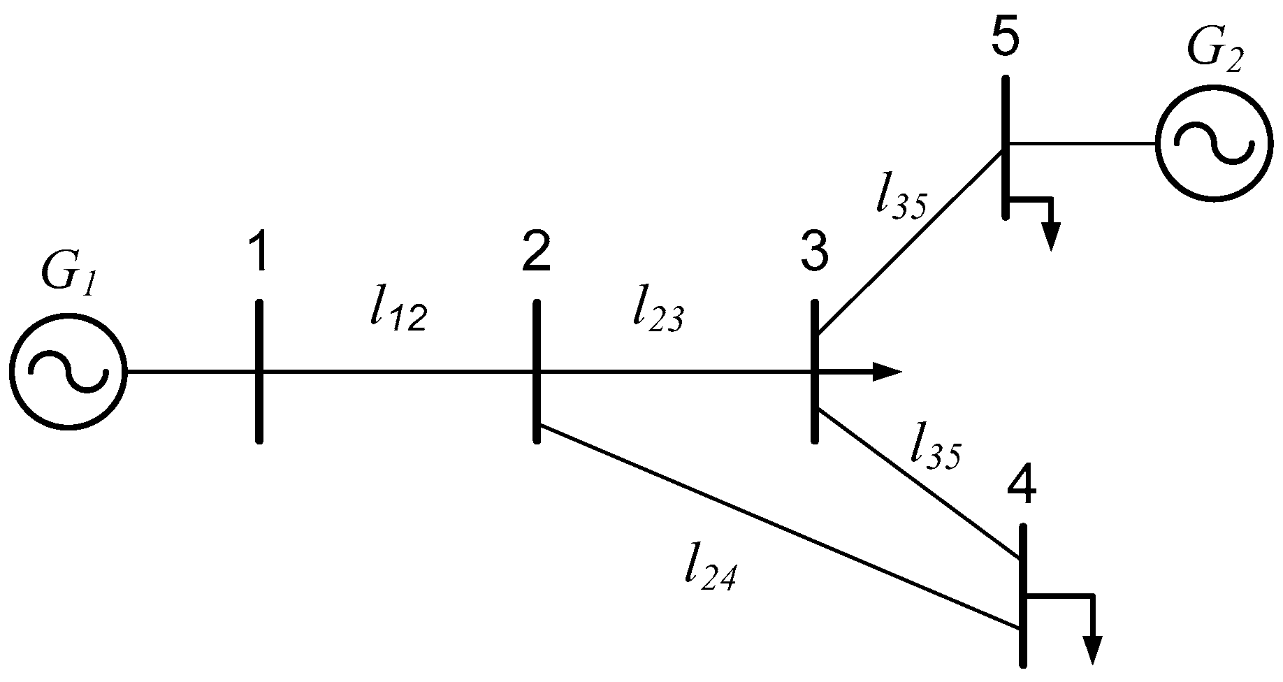
4.1. Results of Simulation for Two5-Bus System

A five-bus power network is demonstrated in Figure 3 for validation purposes. The data for the lines and buses are provided in Table 1 and Table 2, respectively. There are two configurations to consider:
  • In Figure 3, G2 and l24 are out of operation, creating a radial topology;
  • In Figure 3, G2 and l24 are in operation, forming a meshed structure.
The five-bus system results in a radial topology when G2 and l24 are out of operation. Table 3 indicates the system voltage stability indexes for this radial structure as the system load increases. As λ approaches to the value of 2.11 or the network load is raised to 211 MW, the system eventually loses its voltage stability and this is estimated by CPF method.
It can be observed that the findings of the new suggested method, virtual impedance model methodology, and Thevenin method for detecting system voltage instability are similar with those obtained using CPF when the system is reaching the voltage instability point. The localized voltage stability indices for this radial system when λ approaches to 2.09 are demonstrated in Table 4. In addition to this, λ5 > λ4 > λ3 is sustained. The suggested index located the bus 3, bus 4, and bus 5 as weak buses and the virtual impedance technique similarly identified the bus 3, bus 4, and bus 5 as weak buses. However, as the system approaches its point of instability, the Thevenin technique cannot accurately identify the instability of the system because the system index at the point of instability is faraway from 1.00. The margin of voltage stability of the system can be enhanced from 1.02 to 1.15 by adding 40 Mvar shunt capacitors to bus 3, bus 4, or bus 5, respectively, and this is in accordance with the three weak buses indicated by the new approach and virtual impedance technique. The margin of voltage stability of the network can be improved from 1.02 to 1.47 by including a line in parallel with l23, however incorporating a line in parallel with l34 or l35 has no effect on the stability margin or bus indexes of the network. This suggests that the bus 3 is the weakest bus and this finding is in accordance with the newly proposed method. The proposed index has efficiently identified the stability margin of the system and determined the location of weak buses in this situation.
When G2 and l24 are in operation, the five-bus system forms a loop network with two generators. Table 5 shows the indices of the voltage stability for this loop system as the load increases in the network. When the load of the network increases to 504 MW the value of λ reaches to 6.30 and the system voltage becomes instable. It can be observed that the findings of the voltage instability of the network estimate by the new proposed index are compatible with CPF technique as the system approaches to voltage instability condition. The virtual impedance technique and the Thevenin method do not accurately measure the voltage instability of the system as the system approaches to the point of instability because the system index at the point of instability is faraway from 1.00. However, the proposed index has accurately identified the system voltage instability and is also consistent with CPF.
When the load level of the system approached λ = 6.25, the newly proposed index identified bus 3 as a weak bus. The stability margin of the network can be enhanced from 1.02 to 1.15 by connecting 120 Mvar shunt capacitors with bus 3 and this is in accordance with the weak bus detected by the new technique.
By connecting a line in parallel with l23, the margin of system voltage stability may be increased from 1.02 to 1.23, which is compatible with the new method’s identification of a weak bus.
The approach, as presented, will be able to detect the voltage fluctuations in the five-bus system, as well as determine where the bus is weak. The above simulation results for a simple five-bus system reveal that the proposed index has accurately identified voltage stability margin as compared to virtual impedance model and Thevenin techniques. It also shows that the proposed index is simple and easy to use in estimating the voltage instability in power systems.

4.2. Findings of the IEEE Systems and a Real 1010-Bus System via Simulations

The proposed technique was tested on four IEEE systems and the Guangdong Electric Power Company’s 1010-bus system in China. Table 6 shows the findings of the voltage stability investigation. The given λ value here is close to the point of instability. The results of system voltage fluctuations determined by the new method are consistent with those attained by CPF, indicating that the new index can efficiently determine the system voltage stability problems for the four IEEE systems and the actual utility system of 1010-bus, as shown in the columns of ‘system index’ below the ‘original system’ of Table 6.
A reference is made to the low load bus of four IEEE systems and one actual 1010 bus system in the column ‘weak buses identified by new method’ of Table 6 ‘original system’. To validate the efficiency of the weak buses identified by the new indicator, the systems are upgraded by applying shunt capacitors or parallel branches to weak buses as shown below:
  • The 14-bus system (IEEE): shunt capacitors of 20 Mvar added to bus 14;
  • The 30-bus system (IEEE): shunt capacitors of 5 Mvar added to bus 30;
  • The 39-bus system (IEEE): shunt capacitors of 10 Mvar added to bus 8;
  • The 57-bus system (IEEE): shunt capacitors of 5 Mvar added to bus 31;
  • Utility system of 1010-bus: shunt capacitors of 15 Mvar added to bus 710.
The indicators of the improved systems acquired by utilizing CPF are listed in Table 6 under the column “enhanced systems”. It can be observed that the system index is much higher than the initial load level, resulting in voltage fluctuations, that is, after various improvements to the identified low load bus, the voltage stability of each system has been greatly improved. This ensures the efficiency of the new method in identifying weak positions. Table 7 lists the number of weak buses detected using the virtual impedance methodology and the recently suggested method for the 1010-bus utility system, together with their respective voltage stability thresholds. The virtual impedance technique can also accurately identify the system voltage fluctuations of four IEEE systems and the real 1010 bus common system, as illustrated in Table 7. Though, the quantities of the weak load buses identified at various voltage stability thresholds are larger than those estimated by the newly proposed technique in Table 7. This shows that the virtual impedance model provides a large number of potential weak buses for operators and organizers. In reality, the improvement of several weak buses acknowledged by the virtual impedance method cannot enhance the stability of system voltage. So, as compared to the virtual impedance model and Thevenin method, the proposed index locates weak-load buses more effectively and provides better estimation of voltage instability. Furthermore, the above simulation also shows that proposed index is simple and easy to utilize for estimation of long-term voltage instability in power systems.

5. Conclusions

This paper has presented a new voltage stability index based on single port equivalent depending on component peculiarity representation and sensitivity persistence. The corresponding equivalent parameters were derived according to the state information of a single system. The susceptibility of bus terminal voltage to bus terminal injection current before and after equivalence was constant, which actually represented the comparability of different types of components. These features further increased the accuracy of voltage stability evaluation based on local bus. Using the novel single port equivalent technique, the new index of system voltage stability was estimated and the locations of the weak load buses were also calculated, in which the improvement strategy greatly enhanced the stability of system voltage. In order to illustrate the efficiency of the proposed equivalent technique and its corresponding indicators, simulations were performed based on four IEEE systems, two radial systems, and a real power system with 5 to 1010-buses. The simulation results obtained for the new index were compared with virtual and Thevenin equivalent models. The proposed model quickly identified the instability of the various power systems by reaching the threshold of value ε = 1 compared with virtual and Thevenin techniques. Additionally, at various thresholds (ε = 1.02, 1.05, 1.10, 1.15) for actual 1010-bus Guangdong system, the new index identified a smaller number of weak buses (4, 4, 8, 14) as compared with the virtual impedance technique (4, 36, 96, 186). These simulation findings has proven the accuracy of the proposed index and it can be used to locate and determine the long-term voltage instability of power networks.

Author Contributions

Conceptualization, M.S.B. and H.L.; methodology, L.I.; software, M.S.; validation, H.L., L.I., and M.S.; formal analysis, Z.u.A.J.; investigation, U.F.; resources, J.A.S.; data curation, M.S.N.; writing—original draft preparation, M.S.B.; writing—review and editing, H.L. and G.R.; visualization, G.R.; supervision, L.I.; project administration, H.L.; funding acquisition, L.I. All authors have read and agreed to the published version of the manuscript.

Funding

This research received was funded by NSF of China under Grant 61661018.

Institutional Review Board Statement

Not applicable.

Informed Consent Statement

Not applicable.

Data Availability Statement

The data of current study can be obtained from corresponding author.

Conflicts of Interest

The authors declare no conflict of interest.

References

  1. Abe, S.; Fukunaga, Y.; Isono, A.; Kondo, B. Power System Voltage Stability. IEEE Trans. Power Appar. Syst. 1982, PAS-101, 3830–3840. [Google Scholar] [CrossRef]
  2. Cutsem, T.; Vournas, C. Voltage Stability of Electric Power Systems; Springer: Berlin/Heidelberg, Germany, 1998. [Google Scholar]
  3. Taylor, C.; Erickson, D. Recording and analyzing the July 2 cascading outage [Western USA power system]. IEEE Comput. Appl. Power 1997, 10, 26–30. [Google Scholar] [CrossRef]
  4. Hatziargyriou, N.; Milanovic, J.; Rahmann, C.; Ajjarapu, V.; Canizares, C.; Erlich, I.; Hill, D.; Hiskens, I.; Kamwa, I.; Pal, B.; et al. Definition and Classification of Power System Stability–Revisited & Extended. IEEE Trans. Power Syst. 2021, 36, 3271–3281. [Google Scholar] [CrossRef]
  5. Hong, Y.-H. Fast calculation of a voltage stability index of power systems. IEEE Trans. Power Syst. 1997, 12, 1555–1560. [Google Scholar] [CrossRef]
  6. Pourkeivani, I.; Abedi, M.; Kouhsari, S.M.; Ghaniabadi, R. A Novel Index to Predict the Voltage Instability Point in Power Systems Using PMU-based State Estimation. In Proceedings of the 2020 14th International Conference on Protection and Automation of Power Systems (IPAPS), Tehran, Iran, 31 December 2019–1 January 2020; pp. 99–104. [Google Scholar] [CrossRef]
  7. Chandra, A.; Pradhan, A.K. Online voltage stability and load margin assessment using wide area measurements. Int. J. Electr. Power Energy Syst. 2019, 108, 392–401. [Google Scholar] [CrossRef]
  8. Su, H.-Y.; Liu, C.-W. Estimating the Voltage Stability Margin Using PMU Measurements. IEEE Trans. Power Syst. 2016, 31, 3221–3229. [Google Scholar] [CrossRef]
  9. Ajjarapu, V.; Christy, C. The continuation power flow: A tool for steady state voltage stability analysis. IEEE Trans. Power Syst. 1992, 7, 416–423. [Google Scholar] [CrossRef]
  10. Xu, P.; Wang, X.; Ajjarapu, V. Continuation power flow with adaptive stepsize control via convergence monitor. IET Gener. Transm. Distrib. 2012, 6, 673–679. [Google Scholar] [CrossRef]
  11. Avalos, R.J.; Canizares, C.A.; Milano, F.; Conejo, A. Equivalency of Continuation and Optimization Methods to Determine Saddle-Node and Limit-Induced Bifurcations in Power Systems. IEEE Trans. Circuits Syst. I Regul. Pap. 2008, 56, 210–223. [Google Scholar] [CrossRef]
  12. Nagendra, P.; Dey, S.H.N.; Paul, S. An innovative technique to evaluate network equivalent for voltage stability assessment in a widespread sub-grid system. Int. J. Electr. Power Energy Syst. 2011, 33, 737–744. [Google Scholar] [CrossRef]
  13. Chen, H.; Jiang, T.; Yuan, H.; Jia, H.; Bai, L.; Li, F. Wide-area measurement-based voltage stability sensitivity and its application in voltage control. Int. J. Electr. Power Energy Syst. 2017, 88, 87–98. [Google Scholar] [CrossRef] [Green Version]
  14. Yu, J.; Liu, J.; Li, W.; Xu, R.; Yan, W.; Zhao, X. Limit preserving equivalent method of interconnected power systems based on transfer capability consistency. IET Gener. Transm. Distrib. 2016, 10, 3547–3554. [Google Scholar] [CrossRef]
  15. Wang, Y.; Li, W.; Lu, J. A new node voltage stability index based on local voltage phasors. Electr. Power Syst. Res. 2009, 79, 265–271. [Google Scholar] [CrossRef]
  16. Chebbo, A.; Irving, M.; Sterling, M. Voltage collapse proximity indicator: Behaviour and implications. IEE Proc. C Gener. Transm. Distrib. 1992, 139, 241–252. [Google Scholar] [CrossRef]
  17. Rahman, T.K.A.; Jasmon, G. A new technique for voltage stability analysis in a power system and improved loadflow algorithm for distribution network. In Proceedings of the 1995 International Conference on Energy Management and Power Delivery EMPD ’95, Singapore, 21–23 November 1995. [Google Scholar]
  18. Smon, I.; Verbic, G.; Gubina, F. Local Voltage-Stability Index Using Tellegen’s Theorem. IEEE Trans. Power Syst. 2006, 21, 1267–1275. [Google Scholar] [CrossRef]
  19. Hazarika, D. New method for monitoring voltage stability condition of a bus of an interconnected power system using measurements of the bus variables. IET Gener. Transm. Distrib. 2012, 6, 977–985. [Google Scholar] [CrossRef]
  20. Jiang, T.; Bai, L.; Jia, H.; Yuan, H.; Li, F. Identification of voltage stability critical injection region in bulk power systems based on the relative gain of voltage coupling. IET Gener. Transm. Distrib. 2016, 10, 1495–1503. [Google Scholar] [CrossRef]
  21. Kessel, P.; Glavitsch, H. Estimating the Voltage Stability of a Power System. IEEE Trans. Power Deliv. 1986, 1, 346–354. [Google Scholar] [CrossRef]
  22. Zhao, J.; Yang, Y.; Gao, Z. A review on on-line voltage stability monitoring indices and methods based on local phasor measurements. In Proceedings of the 17th Power Systems Computation Conference, Stockholm, Sweden, 22–26 August 2011. [Google Scholar]
  23. Wang, Y.; Pordanjani, I.R.; Li, W.; Xu, W.; Chen, T.; Vaahedi, E.; Gurney, J. Voltage Stability Monitoring Based on the Concept of Coupled Single-Port Circuit. IEEE Trans. Power Syst. 2011, 26, 2154–2163. [Google Scholar] [CrossRef]
  24. Li, W.; Chen, T.; Xu, W. On impedance matching and maximum power transfer. Electr. Power Syst. Res. 2010, 80, 1082–1088. [Google Scholar] [CrossRef]
  25. Li, W.; Wang, Y.; Chen, T. Investigation on the Thevenin equivalent parameters for online estimation of maximum power transfer limits. IET Gener. Transm. Distrib. 2010, 4, 1180–1187. [Google Scholar] [CrossRef]
  26. Van Amerongen, R.; Van Meeteren, H.P. A Generalised Ward Equivalent for Security Analysis. IEEE Trans. Power Appar. Syst. 1982, PAS-101, 1519–1526. [Google Scholar] [CrossRef]
  27. Yu, J.; Zhang, M.; Zhu, L.; Yan, W.; Zhao, X. New theory on external network static equivalent based on sensitivity consistency. Zhongguo Dianji Gongcheng Xuebao/Proc. Chin. Soc. Electr. Eng. 2013, 35, 3231–3238. [Google Scholar]
  28. Li, W. Probabilistic Transmission System Planning; IEEE: Piscataway, NJ, USA, 2011. [Google Scholar]
  29. Yu, J.; Li, W.; Yan, W.; Zhao, X.; Ren, Z. Evaluating risk indices of weak lines and buses causing static voltage instability. In Proceedings of the IEEE Power and Energy Society General Meeting-Conversion and Delivery of Electrical Energy in the 21st Century 2011, Detroit, MI, USA, 24–28 July 2011; pp. 1–7. [Google Scholar]
Figure 1. Single-port equivalent depending on component peculiarity representation and sensitivity persistence for bus j.
Processes 09 01849 g001
Figure 2. Stepwise chart for determining weak buses to monitor voltage instability.
Processes 09 01849 g002
Figure 3. Five-bus system.
Processes 09 01849 g003
Table 1. Bus information of the five-bus system.
BusLoad, MVAVoltage Magnitude, p.u.Voltage Angle
101.060
201-
360 + j40--
420 + j10--
520 + j10--
Table 2. Line data in the five-bus system.
LineFrom Bus NumberTo Bus NumberImpedance, p.u.
l12120.02 + j0.04
l23230.03 + j0.07
l24240.05 + j0.09
l34340.03 + j0.07
l35350.01 + j0.02
Table 3. Voltage stability system indices for the radial five-bus network with G2 and l24 out of operation when all loads increase.
ΛSystem Loads
MW
System Index
New Proposed
Model
Virtual Impedance ModelThevenin Impedance Model
1.081082.171.93.32
1.191191.861.733.01
1.281281.71.612.8
1.391391.551.482.58
1.481481.431.392.42
1.591591.351.312.26
1.681681.271.232.12
1.791791.151.162
1.891891.091.111.9
1.981981.041.061.81
2.092091.011.021.71
2.11211111.69
Table 4. Voltage stability local indices for the radial five-bus system with G2 and l24 out of operation when λ = 2.09.
λSystem Loads, MWProposed Equivalent ModelVirtual Impedance ModelThevenin Impedance Model
Bus 3Bus 4Bus 5Bus 3Bus 4Bus 5Bus 3Bus 4Bus 5
2.092091.011.241.851.051.021.041.713.574.85
Table 5. Voltage stability system indices for the loop topology of five-bus system with G2 and l24 in operation as all loads increase.
λSystem Loads
MW
System Index
New Proposed ModelVirtual Impedance ModelThevenin Impedance Model
1.2910312.399.4515.91
1.5812610.037.7613.06
2.11688.015.689.54
3.62884.513.065.17
4.793832.652.073.46
5.284222.061.752.88
5.984781.291.342.11
6.154921.111.251.92
6.24961.051.221.87
6.255001.021.191.81
6.350411.171.75
Table 6. Results of voltage stability analysis for the four IEEE systems and the 1010-bus utility system before and after enhancements.
SystemSelected Buses with Load IncreasingλSystem IndexWeak Buses Identified by New MethodEnhanced SystemSystem Index Identified by CPF
New Proposed ModelVirtual Impedance ModelThevenin Impedance Model
IEEE 14-bus systemall load buses3.971.001.041.86144.01
IEEE 30-bus systembus 26, 29, 303.71.001.091.4729, 303.80
IEEE 39-bus systemall load buses2.21.001.002.274, 82.31
IEEE 57-bus systemall load buses1.81.011.002.6931, 331.89
Actual 1010-bus Guangdong systemall load buses1.91.001.041.5356, 164, 709, 7102.05
Table 7. Number of the weak load buses for the 1010-bus utility system with the different voltage stability thresholds.
Threshold εThe Number of Weak Load Buses
New MethodVirtual Impedance
1.0244
1.05436
1.10896
1.1514186
Publisher’s Note: MDPI stays neutral with regard to jurisdictional claims in published maps and institutional affiliations.

