
Energy Flexibility Chances for the Wastewater Treatment Plant of the Benchmark Simulation Model 1

 and
and
Abstract
:1. Introduction
2. Methods and Approach
2.1. Benchmark Simulation Model 1 and User-Defined Control Strategies under Study
2.2. Energy Market in Germany and Analysis of Energy Consumption Data
3. Simulations and Discussion
3.1. Control Strategies: No-Energy-Flexibility Scenario
3.2. Energy Flexibility Scenarios
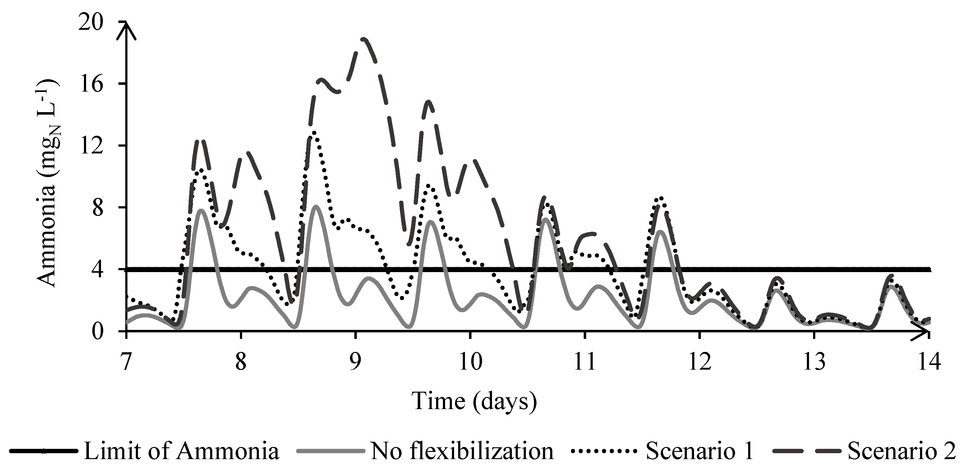
3.2.1. Scenario 1: Undetermined On/Off Aeration Cycle
3.2.2. Scenario 2: Predetermined On/Off Aeration Cycle
3.3. Aggregated Results and Final Discussion
4. Conclusions
Author Contributions
Funding
Institutional Review Board Statement
Informed Consent Statement
Conflicts of Interest
References
- Schäfer, M.; Hobus, I.; Schmitt, T.G. Energetic flexibility on wastewater treatment plants. Water Sci. Technol. 2017, 76, 1225–1233. [Google Scholar] [CrossRef]
- Bublitz, A.; Keles, D.; Zimmermann, F.; Fraunholz, C.; Fichtner, W. A Survey on Electricity Market Design: Insights from Theory and Real-World Implementations of Capacity Remuneration Mechanisms; Working Paper Series in Production and Energy; Karlsruhe Institute of Technology (KIT); Institute for Industrial Production (IIP): Karlsruhe, Germany, 2018; No. 27. [Google Scholar]
- Brok, N.B.; Munk-Nielsen, T.; Madsen, H.; Stentoft, P.A. Flexible control of wastewater aeration for cost-efficient, sustainable treatment, IFAC Workshop on Control of Smart Grid and Renewable Energy Systems. IFAC PapersOnLine 2019, 52, 494–499. [Google Scholar] [CrossRef]
- Fallahi, Z.; Henze, G.P. Interactive buildings: A review. Sustainability 2019, 11, 3988. [Google Scholar] [CrossRef] [Green Version]
- Schäfer, M. Short-term flexibility for energy grids provided by wastewater treatment plants with anaerobic sludge digestion. Water Sci. Technol. 2020, 81, 1388–1397. [Google Scholar] [CrossRef] [PubMed]
- Chen, S.; Härdle, W.K.; López Cabrera, B. Regularization Approach for Network Modeling of German Energy Market; IRTG 1792 Discussion Paper 2018-017; Humboldt University of Berlin: Berlin, Germany, 2018. [Google Scholar]
- Seier, M.; Schebek, L. Model-based investigation of residual load smoothing through dynamic electricity purchase: The case of wastewater treatment plants in Germany. Appl. Energy 2017, 205, 210–224. [Google Scholar] [CrossRef]
- Bertsch, J.; Growitsch, C.; Lorenczik, S.; Nagl, S. Do We Need an Additional Flexibility Market in the Electricity System?—A System-Economic Analysis for EUROPE; Paper based on the study: Flexibility options in European Electricity Markets in high RES-E Scenarios, for the International Energy Agency; Institute of Energy Economics, University of Cologne: Köln, Germany, 2013. [Google Scholar]
- Yilmaz, S.; Xu, X.; Cabrera, D.; Chanez, C.; Cuony, P.; Patel, M.K. Analysis of demand-side response preferences regarding electricity tariffs and direct load control: Key findings from a Swiss survey. Energy 2020, 212, 118712. [Google Scholar] [CrossRef]
- Langendahl, P.-A.; Roby, H.; Potter, S.; Cook, M. Smoothing peaks and troughs: Intermediary practices to promote demand side response in smart grids. Energy Res. Soc. Sci. 2019, 58, 101277. [Google Scholar] [CrossRef]
- Ford, J.J.; Bevrani, H.; Ledwich, G. Adaptive load shedding and regional protection. Int. J. Electr. Power Energy Syst. 2009, 31, 611–618. [Google Scholar] [CrossRef]
- Balakumar, P.; Sathiya, S. Demand side management in smart grid using load shifting technique. In Proceedings of the 2017 International Conference on Electrical, Instrumentation and Communication Engineering (ICEICE2017), Karur, India, 27–28 April 2017. [Google Scholar]
- Schäfer, M.; Gretzschel, O.; Steinmetz, H. The possible roles of wastewater treatment plants in sector coupling. Energies 2020, 13, 2088. [Google Scholar] [CrossRef] [Green Version]
- Aymerich, I.; Rieger, L.; Sobhani, R.; Rosso, D.; Corominas, L.L. The difference between energy consumption and energy cost: Modelling energy tariff structures for water resource recovery facilities. Water Res. 2015, 81, 113–123. [Google Scholar] [CrossRef] [Green Version]
- Larsen, M.A.D.; Drews, M. Water use in electricity generation for water-energy nexus analyses: The European case. Sci. Total Environ. 2019, 651, 2044–2058. [Google Scholar] [CrossRef] [PubMed]
- Schäfer, M.; Gretzschel, O.; Schmitt, T.G.; Knerr, H. Wastewater treatment plants as system service provider for renewable energy storage and control energy in virtual power plants—A potential analysis. Energy Procedia 2015, 73, 87–93. [Google Scholar] [CrossRef] [Green Version]
- Revolar, S.; Vega, P.; Vilanova, R.; Francisco, M. Optimal control of wastewater treatment plants using economic-oriented model predictive dynamic strategies. Appl. Sci. 2017, 7, 813. [Google Scholar] [CrossRef]
- Husin, M.H.; Rahmat, M.F.; Wahab, N.A.; Sabri, M.F.M.; Suhaili, S. Proportional-integral ammonium-based aeration control for activated sludge process. In Proceedings of the 2020 13th International UNIMAS Engineering Conference (EnCon), Kota Samarahan, Malaysia, 27–28 October 2020. [Google Scholar]
- Schraa, O.; Rieger, L.; Alex, J. Development of a model for activated sludge aeration systems: Linking air supply, distribution, and demand. Water Sci. Technol. 2017, 75, 552–560. [Google Scholar] [CrossRef] [Green Version]
- Gretzschel, M.O.; Schäfer, M.; Steinmetz, H.; Pick, E.; Kanitz, E.; Krieger, S. Advanced wastewater treatment to eliminate organic micropollutants in wastewater treatment plants in combination with energy-efficient electrolysis at WWTP Mainz. Energies 2020, 13, 3599. [Google Scholar] [CrossRef]
- Barbose, G.; Goldman, C. A Survey of Utility Experience with Real Time Pricing; LBNL-54238; Lawrence Berkley National Laboratory: Berkeley, CA, USA, 2004. [Google Scholar]
- Alex, J.; Benedetti, L.; Copp, J.; Gernaey, K.V.; Jeppsson, U.; Nopens, I.; Pons, M.N.; Steyer, J.P.; Vanrolleghem, P. Benchmark Simulation Model No. 1 (BSM1); University of Lund: Lund, Sweden, 2008. [Google Scholar]
- Liu, H.; Yoo, C. Cascade control of effluent nitrate and ammonium in an activated sludge process. Desalination Water Treat. 2015, 57, 21253–21263. [Google Scholar] [CrossRef]
- Santín, I.; Pedret, C.; Vilanova, R. Control strategies for ammonia violations removal in BSM1 for dry, rain and storm weather conditions. In Proceedings of the 23rd Mediterranean Conference on Control and Automation (MED), Paper ThAT 2.3, Torremolinos, Spain, 16–19 June 2015. [Google Scholar]
- Mulas, M.; de Araùjo, A.C.B.; Baratti, R.; Skogestad, S. Optimized control structure for a wastewater treatment benchmark. In Proceedings of the 9th International Symposium on Dynamics and Control of Process Systems (DYCOPS 2010), Leuven, Belgium, 5–7 July 2010. [Google Scholar]
- Henze, M.; Grady, C.P.L., Jr.; Gujer, W.; Marais, G.V.R.; Matsuo, T. Activated Sludge No 1, Scientific and Technical Reports No 1; International Association on Water Pollution Research and Control: London, UK, 1987. [Google Scholar]
- Takács, I.; Patry, G.G.; Nolasco, D. A dynamic model of the clarification-thickening process. Water Res. 1991, 25, 1263–1271. [Google Scholar] [CrossRef]
- Vanrolleghem, P.A.; Gillot, S. Robustness and economic measures as control benchmark performance criteria. Water Sci. Technol. 2002, 45, 117–126. [Google Scholar] [CrossRef]
- Stare, A.; Vrečko, D.; Hvala, N.; Strmčnik, S. Comparison of control strategies for nitrogen removal in an activated sludge process in terms of operating costs: A simulation study. Water Res. 2007, 41, 2004–2014. [Google Scholar] [CrossRef] [PubMed]
- Gernaey, K.V.; Jeppsson, U.; Vanrolleghem, P.A.; Copp, J.B. Benchmarking of Control Strategies for Wastewater Treatment Plants; Scientific and Technical Report, No. 23, IWA Task Group on Benchmarking of Control Strategies for Wastewater Treatment Plants; IWA Publishing: London, UK, 2014. [Google Scholar]
- Gernaey, K.V.; Vrecko, D.; Rosen, C.; Jeppsson, U. BSM1 versus BSM1_LT: Is the control strategy performance ranking maintained? In Proceedings of the 7th International IWA Symposium on Systems Analysis and Integrated Assessment in Water Management, Washington, DC, USA, 7–9 May 2007. [Google Scholar]
- Morales, J.M.; Conejo, A.J.; Madsen, H.; Pinson, P.; Zugno, M. Balancing Markets. In Integrating Renewables in Electricity Markets, Operational Problems; Springer: New York, NY, USA, 2014; Chapter 4; pp. 101–136. [Google Scholar]
- KU Leuven Energy Institute. EI Fact Sheet: The Current Electricity Market Design in Europe; EI-FACT SHEET 2015-01; KU Leuven Energy Institute: Leuven, Belgium, 2015. [Google Scholar]
- Erbach, G. Understanding Electricity Markets in the EU; Members’ Research Service PE 593.519; European Parliamentary Research Service: Brussels, Belgium, 2016. [Google Scholar]
- Van der Veen, R.A.C.; Hakvoort, R.A. The electricity balancing market: Exploring the design challenge. Util. Policy 2016, 43, 186–194. [Google Scholar] [CrossRef] [Green Version]
- Mazzi, N.; Pinson, P. Wind power in electricity markets and the value of forecasting. In Renewable Energy Forecasting, From Models to Applications; Woodhead Publishing Series in Energy; Woodhead Publishing: Sawston, UK, 2017; pp. 259–278. [Google Scholar]
- Home|EPEX SPOT. Available online: https://www.epexspot.com/en (accessed on 15 April 2021).
- Khoshrou, A.; Pauwels, E.J.; Dorsman, A.B. The evolution of electricity price on the German day-ahead market before and after the energy switch (CEVI). Renew. Energy 2019, 134, 1–13. [Google Scholar] [CrossRef] [Green Version]
- Maciejowska, K.; Nitka, W.; Weron, T. Day-ahead vs. intraday-Forecasting the price spread to maximize economic benefits. Energies 2019, 12, 631. [Google Scholar] [CrossRef] [Green Version]
- BMWi. Available online: https://www.bmwi.de/Navigation/DE/Home/home.html (accessed on 15 April 2021).


| Controllers | Description |
|---|---|
| DO | DO concentration control by manipulating kLa through aeration |
| NO3-N | Nitrate nitrogen concentration control by manipulating internal recirculation flowrate |
| NH4-N | Ammonia concentration control by manipulating the DO set point in the DO loop (cascade control) |
| Strategy | DO | NO3-N | NH4-N | |||
|---|---|---|---|---|---|---|
| Location | SP (mgO2 L−1) | Location | SP (mgN L−1) | Location | SP (mgN L−1) | |
| Strategy 1 | Tank 5 | 2 | Tank 1 | 1 | — | |
| Strategy 2 | Tanks 3, 4, and 5 | 2 | Tank 1 | 1 | — | |
| Strategy 3 | Tanks 3, 4, and 5 | 2 | — | — | — | |
| Strategy 4 | Tanks 3, 4, and 5 | 0–4 | Tank 1 | 1 | Tank 5 | 1 |
| Strategy 5 | Tanks 3, 4, and 5 | 0–4 | — | — | Tank 5 | 1 |
| Strategy 6 | Tanks 3, 4, and 5 | 0–4 | Tank 1 | 1 | Tank 5 | 3.5 |
| Strategy 7 | Tanks 3, 4, and 5 | 0–4 | — | — | Tank 5 | 3.5 |
| Scenario 1 | Scenario 2 | |
|---|---|---|
| Flexibilization option | Complete aeration shut-off | Intermittent aeration (one hour cycle with 30 min off and 30 min on) |
| Minimum air flow during shut-off | kLa ≥ 20 d−1 | kLa ≥ 20 d−1 |
| Affected tanks of BSM1 | Tanks 3, 4, and 5 | Tanks 3, 4, and 5 |
| Condition regarding effluent quality | Effluent ammonia concentration below 4 mgN L−1 | No condition |
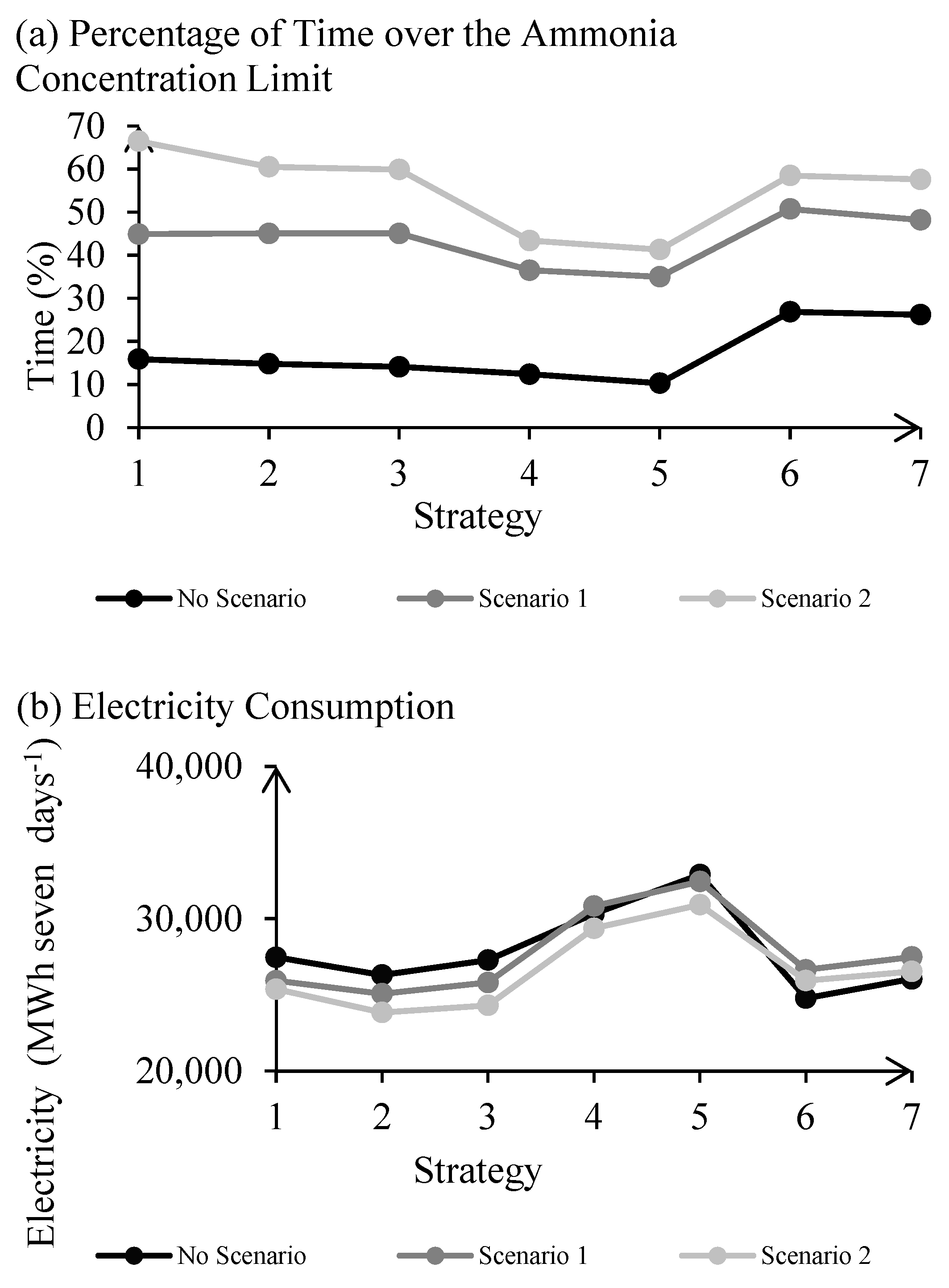
| Strategy | Percentage of Time over the Ammonia Concentration Limit | Energy Consumption (MWh over 7 Days) |
|---|---|---|
| 1 | 15.9 | 27,466.7 |
| 2 | 14.8 | 26,299.3 |
| 3 | 14.1 | 27,280.8 |
| 4 | 12.4 | 30,319.5 |
| 5 | 10.3 | 32,895.7 |
| 6 | 26.9 | 24,774.8 |
| 7 | 26.2 | 26,043.6 |
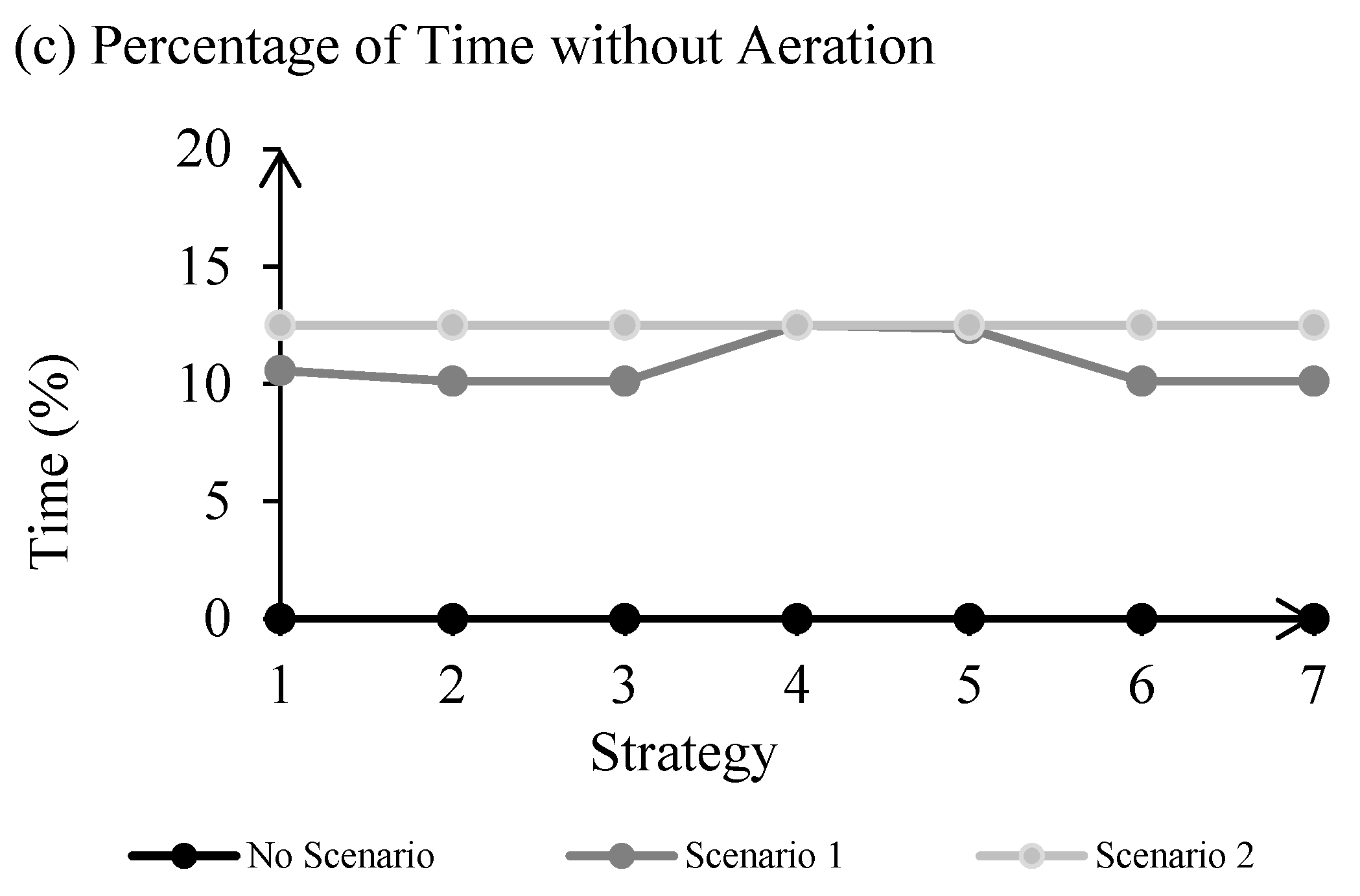
| Strategy | Percentage of Time over the Ammonia Concentration Limit | Energy Consumption (MWh over 7 Days) | Percentage of Time of No Aeration |
|---|---|---|---|
| 1 | 44.91 | 25,930.5 | 10.57 |
| 2 | 45.06 | 25,074.7 | 10.12 |
| 3 | 45.06 | 25,806.7 | 10.12 |
| 4 | 36.53 | 30,828.1 | 12.50 |
| 5 | 35.01 | 32,436.1 | 12.35 |
| 6 | 50.75 | 26,641.4 | 10.12 |
| 7 | 48.20 | 27,487.7 | 10.12 |
| Strategy | % of Time over the Ammonia Concentration Limit | Energy Consumption (MWh over 7 Days) |
|---|---|---|
| 1 | 66.47 | 25,367.5 |
| 2 | 60.48 | 23,838.9 |
| 3 | 59.88 | 24,309.7 |
| 4 | 43.41 | 29,369.6 |
| 5 | 41.32 | 30,923.2 |
| 6 | 58.53 | 25,930.8 |
| 7 | 57.63 | 26,531.3 |
Publisher’s Note: MDPI stays neutral with regard to jurisdictional claims in published maps and institutional affiliations. |
© 2021 by the authors. Licensee MDPI, Basel, Switzerland. This article is an open access article distributed under the terms and conditions of the Creative Commons Attribution (CC BY) license (https://creativecommons.org/licenses/by/4.0/).
Share and Cite
Skouteris, G.; Parra Ramirez, M.A.; Reinecke, S.F.; Hampel, U. Energy Flexibility Chances for the Wastewater Treatment Plant of the Benchmark Simulation Model 1. Processes 2021, 9, 1854. https://0-doi-org.brum.beds.ac.uk/10.3390/pr9101854
Skouteris G, Parra Ramirez MA, Reinecke SF, Hampel U. Energy Flexibility Chances for the Wastewater Treatment Plant of the Benchmark Simulation Model 1. Processes. 2021; 9(10):1854. https://0-doi-org.brum.beds.ac.uk/10.3390/pr9101854
Chicago/Turabian StyleSkouteris, George, Mario Alejandro Parra Ramirez, Sebastian Felix Reinecke, and Uwe Hampel. 2021. "Energy Flexibility Chances for the Wastewater Treatment Plant of the Benchmark Simulation Model 1" Processes 9, no. 10: 1854. https://0-doi-org.brum.beds.ac.uk/10.3390/pr9101854