Pairing Experimental and Mathematical Modeling Studies on Fluidized Beds for Enhancement of Models Predictive Quality: A Current Status Overview

Abstract

Modeling of gas-solid fluidized systems has been a prevailing challenge over the last few decades. With different approaches and implementing different sub-models to capture the essential multiphase and multiscale phenomena in these systems, major advances have been achieved, even though most models are only subject to a practical validation of macroscopic parameters. The current description of fluidized beds through mathematical models relies on the inclusion of vast sub-models, leading to an unquantifiable degree of uncertainty on the models’ applicability for extrapolation studies. Furthermore, each closure and fitting parameter in the model represents a possible source of deviation, and their optimization, hence, becomes another major challenge. The recent advances in measurement techniques can enable us to troubleshoot and optimize the implemented models and sub-models based on local scale measurements. Local multiphase hydrodynamic information obtained by advanced measurement techniques can enable the validation of local predictions and optimization of the coupled sub-models, leading to the development of simplified and highly predictive models. Thus, pairing advanced experimental studies on these systems with insightful modeling approaches is required to advance the shortcoming and enhance the predictive quality of the models. In this work, an overview of the status of modeling and experimental measurement techniques for gas-solid fluidized beds is presented; then, an overview on pairing both experimental and modeling studies to improve the models’ local predictions for fluidized beds is presented.

1. Introduction

Gas-solid fluidized bed systems are of great interest in industrial applications, such as Fischer-Tropsch synthesis, CO₂ capture, biomass combustion, gasification, drying and other catalytic processes [1,2,3,4,5]. These systems have been desirable for such vast applications by virtue of their high mass transfer rates due to the high gas-solid contact and intense solids mixing, nearly isothermal temperature distributions even for highly exothermic reactions, and low pressure drops [6,7,8,9].

Despite these vast industrial applications of fluidized beds, the local-scale phenomena, such as the flow structures, mixing behaviors solids trajectories and recirculation inside the bed, are poorly understood [10,11,12,13,14]. To a great extent, the lack of a deeper knowledge of the local-scale phenomena on these systems lies on the complexity of the multiphase and multiscale interactions, and the recognized scale dependency of these systems [15,16,17]. Remarkably, it has been reported on the literature that the gas-phase dynamics is scale-dependent and is affected by textural characteristics of the bed, such as the column diameter to average the solid particle diameter ratio $\left(D_{\mathrm{C}}/\langle D_{\mathsf{\sigma }}\rangle \right)$, the solid particles material and size, and the presence of internal structures [6,8,18,19,20,21]. This disadvantageous characteristic of the hydrodynamic behavior of fluidized beds will be prevalent in reactors of different length scales, and will affect key parameters, such as bubble size, bubble rise velocity, bubble trajectories, bubble growth and mass transfer of reactants from the bubbling gas-phase to the disperse solids phase.

Vast experimental studies have been conducted to characterize the key hydrodynamic and design parameters of fluidized beds, in order to identify the conditions and phenomena that have adverse effects on the two-phase hydrodynamic phenomena, kinetic throughput, and thermal behavior [22,23,24]. However, most of the applied experimental techniques have important limitations in the level of detail and accuracy in the description of the local scale phenomena and are limited to a restricted number of locations inside the bed [25], only allowing us to measure macroscopic parameters, such as implementing absolute or differential pressure transducers [26], or fail to provide detailed time resolved measurements of the local fields [14]. This represents a fundamental limitation when characterizing the hydrodynamics of chaotic fluidized systems, such as FB reactors where strong pointwise and timewise variations of the local fields have been observed [20,27]. Furthermore, systematic errors depending on the implemented measurement technique have been observed [11], such as the disturbance of particle velocities when inserting optical fiber sensors [28]. Considering that the key hydrodynamic parameters in fluidized beds are interrelated gas-solid parameters, such as holdups distribution and bubble properties, measurement techniques that disturb the solids dynamics will also affect gas phase measurements.

Hence, a comprehensive and detailed characterization and prediction of the pointwise and timewise hydrodynamic behavior of gas-solid fluidized systems is still required and is of paramount importance for troubleshooting and optimization of current systems, as well as for the design, scale up tasks and the implementation of new processes. There is still a need to fulfill the shortcomings in the knowledge of the local-scale phenomena in fluidized systems, as well as to develop tools to predict the macroscopic and pointwise behavior of these systems and to optimize, troubleshoot, design, and scale-up. A promising alternative to advance the knowledge of the local-scale phenomena is the application and development of locally validated mathematical models, which enable the timewise and pointwise analysis of hydrodynamics phenomena and extrapolation studies. However, nowadays, the modeling of these systems requires simplifications, such as model order reduction, since the purely theoretical (mechanistic) models are still too computationally expensive, require an unpractical level of detail in the geometrical representation [29], or result in ill-posed or highly stiff equations [30]. In order to avoid such complexity, the common approach is to insert on the transport equations closure sub-models that capture, to a certain extent, complex phenomena, such as the microscale multiphase interactions [31]. The drawback in relying on coupled sub-model lays is the fact that these closure terms are usually a set of empirical or semi-empirical expressions, which lack a mechanistic development and can, hence, constrain the applicability of the main mathematical model. Furthermore, the coupled sub-models usually lack an independent validation, and are instead usually tied to a practical validation by virtue of a validation procedure of the main model [32].

Accordingly, despite the advantages that mathematical modeling can provide in advancing the knowledge of local scale phenomena on these systems, there is still a shortcoming in locally validated models. Furthermore, even though coupling sub-models can enhance the predictive quality of the models, the applicability of a model can be constrained by the applicability of the sub-models, so that a predictive model that relies on a vast number of coupled sub-models could potentially be closer to a fitting of the model against the presented experimental data, rather than being a predictive model. Hence, in this work, an overview on pairing mathematical modeling studies with detailed local experimental measurements in order to enhance the predictive quality of mathematical models, while keeping a reduced number of coupled sub-models, for a Fluidized Bed is presented.

2. Overview of Mathematical Models for Gas-Solid Fluidized Beds

In the context of modeling gas-solid fluidized beds, two main different approaches can be distinguished, which differ in the treatment of the solid phase. The first approach is considering an Euler-Lagrangian specification of the flow field, where the fluid phase follows an Eulerian frame of reference, and the solid phase a Langrangian [33]. In these models, the fluid phase is considered to be continuous, and is modeled by a Navier–Stokes equation, while the solid phase is considered to be a discrete phase, where every solid particle is resolved, and their movement is modeled by Newton’s Equation of Motion. The Eulerian and Langrangian phases in this approach are coupled through boundary conditions set at each solid surface; other multiphase interactions are incorporated though additional interfacial momentum exchange closure sub-models [34,35]. It has been recognized that Eulerian-Lagrange models, also known as CFD-discrete element models (CFD-DEM), best describe the microscale dynamic behaviors of these systems [36]. However, these models become computationally expensive when dealing with a large number of solid particles, and are, thus, usually constrained to model systems of around 10⁵ particles [34,35]. This represents an important limitation, as the number of solid particles in lab-scale fluidized systems can be around 10⁹. Therefore, CFD-DEM models do not seem to be suitable to model lab-scale or larger scale systems.

In order to deal with the limitation of computational resources, new computational and model order reduction schemes for CFD-DEM models have been proposed in recent years, commonly called unresolved CFD-DEM [37,38,39,40,41,42]. In this approach, there is a pseudo coupling of the phases, by replacing the boundary resovled gas-solid superficial interactions for effective volumetric momentum exchange closures. This allows to set a computational mesh for the gas phase coarser than the solid particles size, where the effective volumetric gas–solid interactions are estimated on each mesh element [41]. With unresolved CFD-DEM models, systems of up to $50\times {10}^6$ have been modeled [42]. However, this approach, in contrast with the resolved CFD-DEM approach, required the coupling of additional sub-models to account for effective multiphase interactions, such as drag force, virtual mass force, and Shaffman and Magnus lift force sub-models [41,43,44]. Other model order reductions for resolved CFD-DEM models have been recently proposed, such as the so-called particle-in-cell (PIC) approach. PIC models consider that the solid particles in a fluidized can be modeled as parcels composed of a finite number of particles, and that the inter-parcel, intra-parcel (intraparticle) and fluid–parcel interactions can be accounted for through the closures implemented on the governing equations [45]. Applying the PIC approach, Ma et al. [46] and Yang et al. [47] reduced the number of resolved particles from 10⁶ to 1.8 × 10⁵ parcels, using parcels of around 60 particles, while Breault et al. [48] used 2.53 × 10⁵ parcels to model 4.63 × 10⁸ solid particles, using parcels of around 1830 particles.

The second approach in modeling these systems is considering an Euler–Euler specification of the flow field, where both phases are treated as continuum interpenetrating phases, by considering the solid phase as a pseudo continuum phase [49]. This approach has been recognized as a promising alternative to the CFD-DEM models, as it allows to model large scale systems, while being computationally efficient, in terms of required computational resources and computing times [36,50]. This approach relies on reducing the model order by simplifying the description of the solid phase; however, such simplification of considering the solid phase to behave as a pseudo-fluid, in essence, overlooks the particle–particle interactions. Therefore, these models require the coupling of sub-models that allow us to incorporate not only the multiphase interactions as in the CFD-DEM models, but also the multiscale particle–particle interactions. This adds further uncertainties in the modeling of these systems, as there is an additional requirement to do a proper selection of the sub-models and their coupling schemes. This approach generally results in models with a vast number of coupled sub-models. The drawback in relying on coupled sub-model lies in the fact that these closure terms are usually a set of empirical or semi-empirical expressions, which lack of a mechanistic development and can, hence, constraint the applicability of the main mathematical model. Furthermore, the coupled sub-models usually lack an independent validation, and are instead usually tied to a practical validation by virtue of a validation procedure of the main model [32].

It can be seen that by either modeling approach, there is a need to model the multiphase and multiscale interactions through the inclusion of sub-models. Hence, developing an insightful and useful mathematical model for fluidized bed systems depends on the selection of the coupled sub-models. Furthermore, considering that each of the coupled sub-models is intended to capture a specific phenomenon in the multiphase flow, each sub-model has a corresponding representative physical length scale, and therefore, a proper selection of the multiscale coupling scheme is needed. For example, the pressure gradient $\left(\nabla P\right)$ has a representative physical length scale corresponding to the reactor length $\left(L_{\mathrm{C}}\right)$ (Equation (1)), since the observable changes in the pressure profiles will be dominant along the axial position of the column [26]; whereas if particle clustering is modeled $\left(\frac{\mathrm{d}{n}_{\mathrm{in}}}{\mathrm{d}t}\right)$ (where $n_{in}$ is the number of particles captured by a cluster), the sub-model will have a representative physical length scale corresponding to the effective collision volume between particles (V) (Equation (2)) [36].

$$O\left(\nabla P\right)\sim O\left(L_{\mathrm{C}}\right)$$

(1)

$$O\left(\frac{\mathrm{d}{n}_{\mathrm{in}}}{\mathrm{d}t}\right)\sim O\left(\mathrm{V}\right)\sim O\left(D_{\mathsf{\sigma }}^3\right)$$

(2)

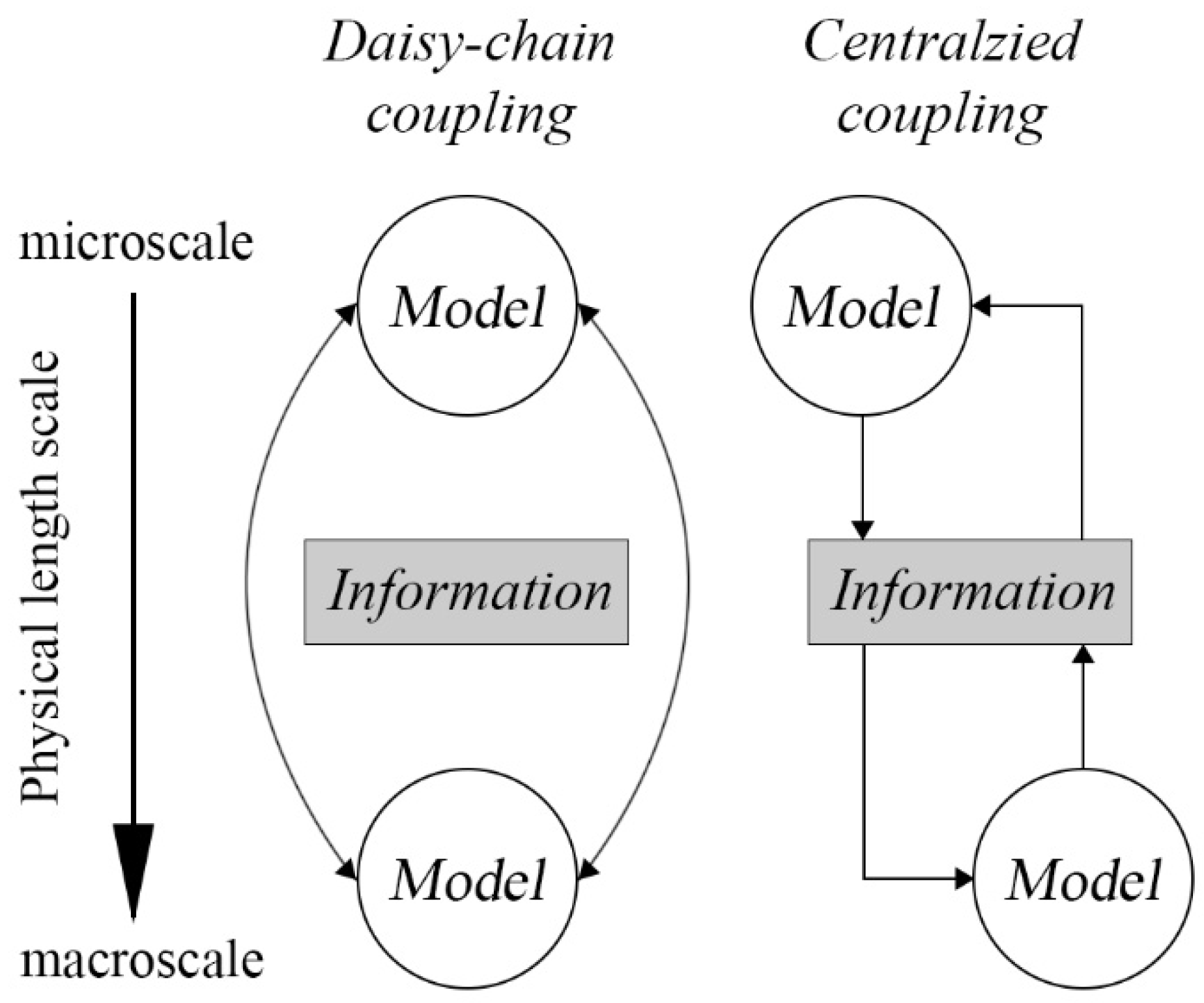
In this sense, two different coupling approaches to incorporate the multiscale interactions through sub-models can be recognized: daisy-chain coupling and centralized coupling [51], (Figure 1). In the daisy-chain coupling, the coupled sub-models to incorporate the multiscale phenomena are simultaneously solved with the main model. In this way, the information of each sub-scale phenomena or sub-model is continuously shared. This kind of multiscale coupling is usually seen in Euler–Euler models that incorporate a Kinetic Theory of Granular Flows (KTGF) approach. Verma et al. [12] implemented an Euler–Euler model for a fluidized bed with two different configurations of internals. In order to model the solid stress tensor, they incorporated a KTGF approach, where they included sub-models to account for granular energy conservation, solids pressure, solids viscosity, and interface momentum transfer.

On the other hand, in a centralized coupling scheme the sub-models are solved in a separated computing step. Information, such as predictions of the flow fields, of the main model are extracted and taken as inputs for the sub-model solver. The sub-models are solved, and their predictions are then extracted and used as inputs to modify the predictions of the main model. This loop is repeated until convergence of the main model is achieved. A clear example of this coupling scheme is seen in models that incorporate a Population Balance Model (PBM). Hu and Liu [36] incorporated a PBM to predict the clustering of solid particles for a fluidized bed. In their modeling scheme, the cluster size distribution estimated by the PBM was used as a closure for the coupled drag force sub-model. The modified estimated drag force improved the predictions of the radial solid holdup distribution and particle velocities.

In every approach considered for gas–solid fluidized systems, there is an underlying requirement of relying in the coupled sub-models and their coupling scheme. Hence, an insightful multiphase flow model will rely on a proper selection of sub-models, which should be based on the underlying assumptions for their derivation and their range of applicability. This implies an added level of uncertainty in the mathematical modeling of these systems that cannot be a priori assessed. Thus, there is a fundamental need to validate the models’ overall and local predictions and assess their predictive quality, which can be achieved by linking models with advanced reliable experiments, which allow us to measure the local hydrodynamic variables. To a great extent, the validation of the models is aimed to measure the deviations in the predictions of the models, rather than pretending to prove the infallibility of the models [32]. The comparison of the local predictions against the local measurements will only provide an outlook on how insightful the implemented model under the tested conditions is. From a rigorous perspective, a model cannot be validated; it can only be claimed that the model is consistent with all the data that its predictions were confronted with [32]. This implies that a different or new set of experiments or data can exhibit a deficiency or limitation in the predictive quality of the model, invalidating the model, or constraining the applicability of the model. Thus, it must be assumed that the validation status of a model may (and will) change over time, and that the models may only be considered to have a practical validation [32,52].

3. Mathematical Modeling

When dealing with an Euler–Euler formulation, also often called two-fluid model (TFM) or Euler-2-Phase (E2P), the most general governing equations for the gas $\left(\beta -phase\right)$ and solid $\left(\sigma -phase\right)$ phases can be described by Equations (3)–(6) [53,54]

$$\frac{\partial \left({\rho }_{\mathsf{\beta }}{\epsilon }_{\mathsf{\beta }}\right)}{\partial t}+\nabla \cdot \left({\rho }_{\mathsf{\beta }}{\epsilon }_{\mathsf{\beta }}{v}_{\mathsf{\beta }}\right)=0$$

(3)

$${\epsilon }_{\mathsf{\beta }}{\rho }_{\mathsf{\beta }}\left[\frac{\partial v_{\mathsf{\beta }}}{\partial t}+v_{\mathsf{\beta }}\cdot \nabla v_{\mathsf{\beta }}\right]={\epsilon }_{\mathsf{\beta }}\left[-\nabla P+\nabla \cdot {\tau }_{\mathsf{\beta }}+{\rho }_{\mathsf{\beta }}g\right]+F_{\mathrm{d}}$$

(4)

$$\frac{\partial {\epsilon }_{\mathsf{\sigma }}}{\partial t}+\nabla \cdot \left({\epsilon }_{\mathsf{\sigma }}{v}_{\mathsf{\sigma }}\right)=0$$

(5)

$${\epsilon }_{\mathsf{\sigma }}{\rho }_{\mathsf{\sigma }}\left[\frac{\partial v_{\mathsf{\sigma }}}{\partial t}+v_{\mathsf{\sigma }}\cdot \nabla v_{\mathsf{\sigma }}\right]={\epsilon }_{\mathsf{\sigma }}\left[-\nabla P+\nabla \cdot {\tau }_{\mathsf{\sigma }}+{\rho }_{\mathsf{\sigma }}g\right]-F_{\mathrm{d}}$$

(6)

where Equations (4) and (6) correspond to the continuity equation for the gas and solid phase, respectively. While Equations (4) and (6) are the momentum balances for the gas and solid phase, respectively, which follow a Navier–Stokes formulation.

The gas phase stress tensor $\left({\tau }_{\mathsf{\beta }}\right)$ is modeled straightforwardly, following Newton’s law of viscosity, as shown in Equation (7). On some contributions for turbulent fluidization, the gas phase stress tensor is modified, for example, following a k-ε formulation [55,56]

$${\tau }_{\mathsf{\beta }}={\mu }_{\mathsf{\beta }}\left[\nabla v_{\mathsf{\beta }}+{\left(\nabla v_{\mathsf{\beta }}\right)}^T-\frac{2}{3}\left(\nabla \cdot v_{\mathsf{\beta }}\right)I\right]$$

(7)

On the other hand, for the solid pseudo-phase, two main different approaches have been explored through the last decades: (i) Kinetic Theory of Granular Flows (KTGF) and (ii) Bed elasticity.

3.1. Solids Stress Tensor

The model formulation shown in Equations (3)–(6) is based on considering that the solid phase is a pseudo-phase that behaves like a fluid. The major complexity in this assumption is modeling the solid stress tensor $\left({\tau }_{\mathsf{\sigma }}\right)$, as it should capture the solid–solid interactions and multiscale phenomena. The most common approach nowadays to model this tensor is by relying on the KTGF formulation [57,58,59]. This approach relies on the kinetic gas theory [59,60] to model an effective solids stress tensor, which follows Equation (8).

$${\tau }_{\mathsf{\sigma }}={\mu }_{\mathsf{\sigma },\mathrm{sh}}\left[\nabla v_{\mathsf{\sigma }}+{\left(\nabla v_{\mathsf{\sigma }}\right)}^T-\frac{2}{3}\left(\nabla \cdot v_{\mathsf{\sigma }}\right)I\right]+{\lambda }_{\mathsf{\sigma }}I$$

(8)

$${\mu }_{\mathsf{\sigma },\mathrm{sh}}={\mu }_{\mathsf{\sigma },\mathrm{col}}+{\mu }_{\mathsf{\sigma },\mathrm{kin}}+{\mu }_{\mathsf{\sigma },\mathrm{fr}}$$

(9)

$${\mu }_{\mathsf{\sigma },\mathrm{col}}=0.8{\rho }_{\mathsf{\sigma }}{D}_{\mathsf{\sigma }}{\epsilon }_{\mathsf{\sigma }}{g}_0\left(1-e\right){\left(\frac{{\Theta }_{\mathsf{\sigma }}}{\pi }\right)}^{1/2}$$

(10)

$${\mu }_{\mathsf{\sigma },\mathrm{kin}}=\frac{10{\rho }_{\mathsf{\sigma }}{D}_{\mathsf{\sigma }}{\left({\Theta }_{\mathsf{\sigma }}\pi \right)}^{1/2}}{96\left(1+e\right){\epsilon }_{\mathsf{\sigma }}{g}_0}{\left[1+\frac{4}{5}\left(1+e\right){\epsilon }_{\mathsf{\sigma }}{g}_0\right]}^2$$

(11)

$${\mu }_{\mathsf{\sigma },\mathrm{fr}}=\frac{p_{\mathrm{s}}\sin \left(\theta \right)}{2I_{2\mathrm{D}}^{1/2}}$$

(12)

$${\lambda }_{\mathsf{\sigma }}=\frac{4}{3}{\epsilon }_{\mathsf{\sigma }}{\rho }_{\mathsf{\sigma }}{D}_{\mathsf{\sigma }}{g}_0\left(1-e\right){\left(\frac{{\Theta }_{\mathsf{\sigma }}}{\pi }\right)}^2$$

(13)

Here, ${\mu }_{\mathsf{\sigma },\mathrm{sh}}$ is the solid shear viscosity, which is generally modeled as an addition of a collision, a kinetic and a frictional contribution, as shown in Equation (9). These constitutive relations are sub-models, and are commonly modeled according to Equations (10)–(12) for both fluidized beds and spouted beds [36,61,62]. In these, $g_0$, e, $p_{\mathrm{s}}$ and $I_{2\mathrm{D}}^{}$ are the solid radial distribution function, particle restitution coefficient, solids pressure and second invariant of the deviatoric stress tensor, for which, further closure terms, sub-models or constitutive relations are needed. ${\lambda }_{\mathsf{\sigma }}$ is the solid bulk viscosity, which is another sub-model, commonly modeled according to Equation (13) [63]. ${\Theta }_{\mathsf{\sigma }}$ is a so-called granular temperature, which captures the fluctuation of the kinetic energy of the particles. The most common approach to model the granular temperature is through inclusion of an additional conservation equation (Equation (14)).

$$\frac{3}{2}\left[\frac{\partial }{\partial t}\left({\epsilon }_{\mathsf{\sigma }}{\rho }_{\mathsf{\sigma }}{\Theta }_{\mathsf{\sigma }}\right)+\nabla \cdot \left({\epsilon }_{\mathsf{\sigma }}{\rho }_{\mathsf{\sigma }}{v}_{\mathsf{\sigma }}{\Theta }_{\mathsf{\sigma }}\right)\right]=\left(-p_{\mathrm{s}}I+{\epsilon }_{\mathsf{\sigma }}{\tau }_{\mathsf{\sigma }}\right):\nabla v_{\mathsf{\sigma }}+\nabla \cdot \left(k\nabla {\Theta }_{\mathsf{\sigma }}\right)-\gamma -{\varphi }_{\mathsf{\beta }\mathsf{\sigma }}$$

(14)

where further closure terms and sub-models are required, namely the diffusivity of granular temperature (k), collisional energy dissipation $\left(\gamma \right)$ and the kinetic energy transfer between phases $\left({\varphi }_{\mathsf{\beta }\mathsf{\sigma }}\right)$. Another approach, not as commonly seen for estimating ${\Theta }_{\mathsf{\sigma }}$, is considering a local equilibrium of the dissipated and generated energy, leading to a quadratic algebraic expression, which is solved directly for ${\Theta }_{\mathsf{\sigma }}$ (Equations (15)–(20)).

$${\Theta }_{\mathsf{\sigma }}^{1/2}=\frac{-K_{1\mathsf{\sigma }}{\epsilon }_{\mathsf{\sigma }}{D}_{\mathsf{\sigma },ii}+{\left(K_{1\mathsf{\sigma }}^2{\epsilon }_{\mathsf{\sigma }}^2{D}_{\mathsf{\sigma },ii}^2+4K_{4\mathsf{\sigma }}{\epsilon }_{\mathsf{\sigma }}\left[K_{2\mathsf{\sigma }}{D}_{\mathsf{\sigma },ii}^2+2K_{3\mathsf{\sigma }}\left(D_{\mathsf{\sigma },ij}^{}{D}_{\mathsf{\sigma },ij}^{}\right)\right]\right)}^{1/2}}{2{\epsilon }_{\mathsf{\sigma }}{K}_{4\mathsf{\sigma }}}$$

(15)

$$K_{1\mathsf{\sigma }}=2\left(1+e\right){\rho }_{\mathsf{\sigma }}{g}_0$$

(16)

$$K_{2\mathsf{\sigma }}=\frac{4\left(1+e\right)D_{\mathsf{\sigma }}{\rho }_{\mathsf{\sigma }}{g}_0}{3{\pi }^{1/2}}-\frac{2}{3}{K}_{3\mathsf{\sigma }}$$

(17)

$$K_{3\mathsf{\sigma }}=\frac{D_{\mathsf{\sigma }}{\rho }_{\mathsf{\sigma }}}{2}\left[\frac{{\pi }^{1/2}}{3\left(3-e\right)}\left(\frac{1}{2}\left(3e+1\right)+\frac{2}{5}\left(1+e\right)\left(3e-1\right){\epsilon }_{\mathsf{\sigma }}{g}_0\right)+\frac{8\left(1+e\right){\rho }_{\mathsf{\sigma }}{g}_0}{5{\pi }^{1/2}}\right]$$

(18)

$$K_{4\mathsf{\sigma }}=\frac{12\left(1-e^2\right){\rho }_{\mathsf{\sigma }}{g}_0}{D_{\mathsf{\sigma }}{\pi }^{1/2}}$$

(19)

$$D_{\mathsf{\sigma },ij}^{}=\frac{1}{2}\left(\frac{\partial v_{\mathsf{\sigma },i}}{\partial x_j}+\frac{\partial v_{\mathsf{\sigma },j}}{\partial x_i}\right)$$

(20)

The KTGF approach requires a vast number of closure sub-models and constitutive relations to model the solids stress tensor. Despite the fact this model has been used successfully in the literature, a vast number of coupled sub-models, and their required closure terms, introduce major uncertainties when modeling gas–solid fluidized systems. Furthermore, the validation of most of these sub-models is a practical validation, which implies that the validation of the models is tied together, and hence, the validation status of each of the sub-models cannot be shown.

The second alternative to model the solids stress tensor is the bed elasticity approach [64,65]. This approach, widely used in the early contributions on mathematical modeling of fluidization, is based on considering that the solid pseudo-phase behaves as an elastic body, which can be compressed and expanded [49]. The compression and expansion of the pseudo-phase is considered to be reflected in changes to the solid holdup $\left({\epsilon }_{\mathsf{\sigma }}\right)$. This proportionality can be mathematically expressed by applying the chain rule on the main diagonal components of the solids stress tensor (Equation (21)).

$$\nabla \cdot {\tau }_{\mathsf{\sigma }}=\frac{\partial {\tau }_{xx}}{\partial {\epsilon }_{\mathsf{\beta }}}\frac{\partial {\epsilon }_{\mathsf{\beta }}}{\partial x}+\frac{\partial {\tau }_{yy}}{\partial {\epsilon }_{\mathsf{\beta }}}\frac{\partial {\epsilon }_{\mathsf{\beta }}}{\partial y}+\frac{\partial {\tau }_{zz}}{\partial {\epsilon }_{\mathsf{\beta }}}\frac{\partial {\epsilon }_{\mathsf{\beta }}}{\partial z}={\displaystyle \sum _i\frac{\partial {\tau }_{ii}}{\partial {\epsilon }_{\mathsf{\beta }}}\frac{\partial {\epsilon }_{\mathsf{\beta }}}{\partial x_i}};{\displaystyle \sum _i\frac{\partial {\epsilon }_{\mathsf{\beta }}}{\partial x_i}}=\nabla {\epsilon }_{\mathsf{\beta }}$$

(21)

$${\displaystyle \sum _i\frac{\partial {\tau }_{ii}}{\partial {\epsilon }_{\mathsf{\beta }}}}=-G\left({\epsilon }_{\mathsf{\beta }}\right)$$

(22)

Using the definition of Equation (22), a modulus of elasticity $\left(-G\left({\epsilon }_{\mathsf{\beta }}\right)\right)$ is defined, which captures the changes in the solids stress tensor with respect to the changes in the local gas holdup ${\epsilon }_{\mathsf{\beta }}$. Several moduli of elasticity have been proposed, generally for fine particles [66,67,68,69,70], and follow the generalized form described in Equation (23) [49,71,72].

$$G\left({\epsilon }_{\mathsf{\beta }}\right)/G_0=\exp \left[-c\left({\epsilon }_{\mathsf{\beta }}-{\epsilon }_{\mathsf{\beta }}^{\prime }\right)\right]$$

(23)

where $G_0$ is a unit normalization factor; c is the compaction modulus; and ${\epsilon }_{\mathsf{\beta }}^{\prime }$ is the compaction gas phase volume fraction.

Table 1. Commonly reported Modulus of Elasticity sub-models.

Model	Author	System
$G\left({\epsilon }_{\mathsf{\beta }}\right)=\exp \left[-600\left({\epsilon }_{\mathsf{\beta }}-0.376\right)\right]$	Bouillard et al. [71]	Fluidized bed with immersed obstacle
$G\left({\epsilon }_{\mathsf{\beta }}\right)=-{10}^{-10.5{\epsilon }_{\mathsf{\beta }}+9.0}$	Gidaspow [73]	Fluidized bed
$G\left({\epsilon }_{\mathsf{\beta }}\right)=\exp \left[-500\left({\epsilon }_{\mathsf{\beta }}-0.422\right)\right]$	Gidaspow and Syamlal [70]	Fluidized bed
$G\left({\epsilon }_{\mathsf{\beta }}\right)=\exp \left[-20\left({\epsilon }_{\mathsf{\beta }}-0.62\right)\right]$	Ettehadieh and Gidaspow [67]	Fluidized bed with a jet
$G\left({\epsilon }_{\mathsf{\beta }}\right)=\exp \left[-100\left({\epsilon }_{\mathsf{\beta }}-0.45\right)\right]$	Kuipers et al. [74]	Numerical model of a fluidized bed
$G\left({\epsilon }_{\mathsf{\beta }}\right)=5\times {10}^6\exp \left[-2.03{\epsilon }_{\mathsf{\beta }}\right]$	Kaae [69]	Fluidized bed with pyrolytic carbons, fluidized with helium and hydrocarbon gas.
$G\left({\epsilon }_{\mathsf{\beta }}\right)=1.5\times {10}^{-3}\exp \left[500\left(0.4-{\epsilon }_{\mathsf{\beta }}\right)\right]$	Syamlal and O’Brien [75]	Multiparticle liquid fluidized bed
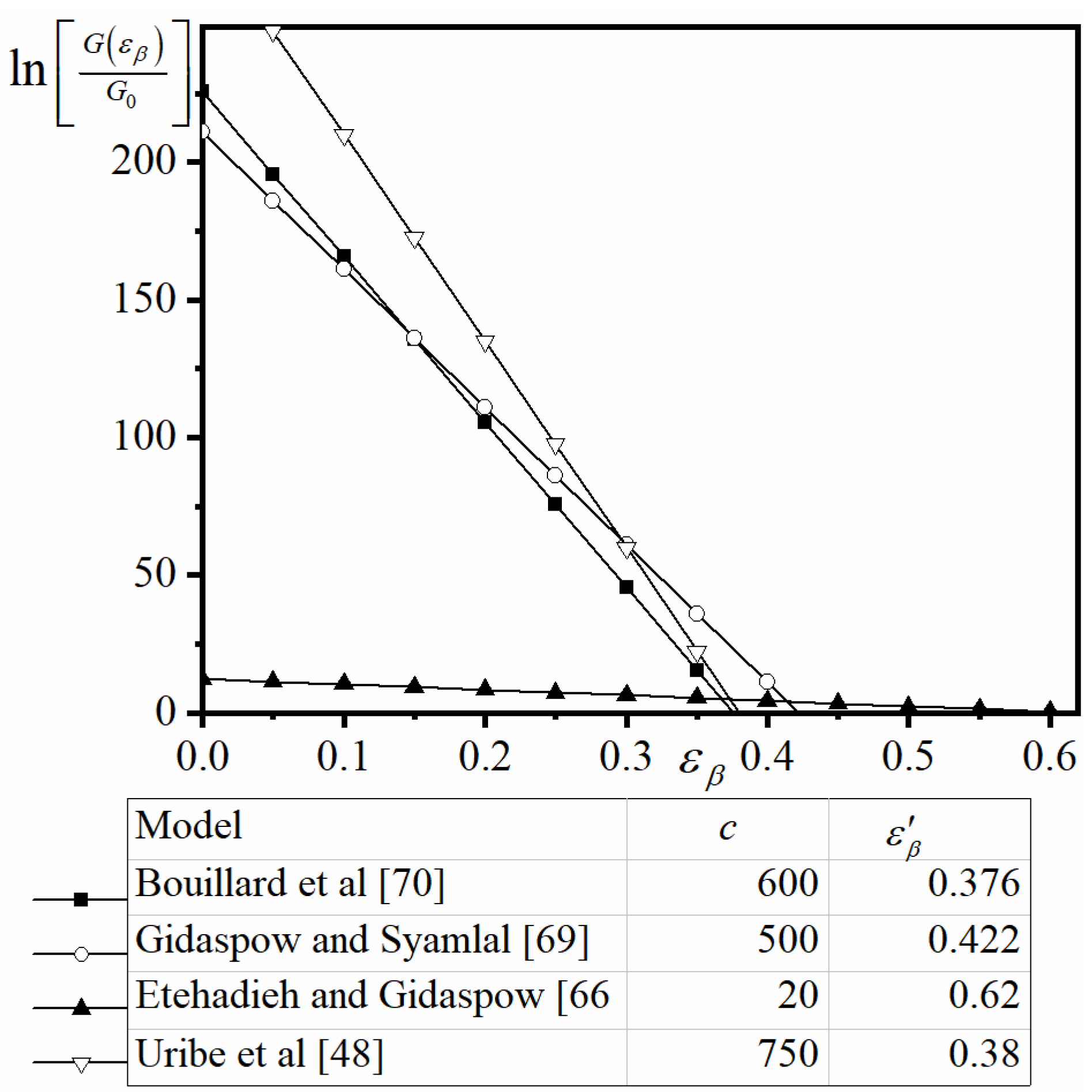
$G\left({\epsilon }_{\mathsf{\beta }}\right)=\exp \left[-750\left({\epsilon }_{\mathsf{\beta }}-0.38\right)\right]$	Uribe et al. [49]	Numerical model of a spouted bed

shows several moduli of elasticity sub-models reported in the literature. Most of these sub-models were developed for fluidized beds, based on separate effect experiments. No specific contributions for other systems dealing with larger particles, such as spouted beds, can be usually found.

As suggested by Uribe et al. [49] and show in Figure 2, the modulus of elasticity sub-models generally makes a strong contribution in the dense regions of the fluidized systems, and tends to zero as the beds get diluted. Hence, an additional pseudo-viscous contribution is included in the solids stress tensor approximation to model the solid–solid interactions in the diluted regions of the bed. Considering this, the solids stress tensor on the bed elasticity approximation is usually modeled according to Equation (24),

$${\epsilon }_{\mathsf{\sigma }}\nabla \cdot {\tau }_{\mathsf{\sigma }}=-G\left({\epsilon }_{\mathsf{\beta }}\right)\nabla {\epsilon }_{\mathsf{\beta }}+{\epsilon }_{\mathsf{\sigma }}\nabla \cdot \left[{\mu }_{\mathrm{eff}}\left(\nabla v_{\mathsf{\sigma }}+{\left(\nabla v_{\mathsf{\sigma }}\right)}^T\right)\right]$$

(24)

where ${\mu }_{\mathrm{eff}}$ is an effective solid pseudo-phase viscosity, for which a sub-model is required. Several models have been proposed since the early contributions on fluidization in order to account for phenomena that might affect the apparent viscosity of the pseudo-phase, such as the model of Frankel and Acrivos that accounts for the proximity effect (Equation (25)), which is suitable for dense bubbling fluidized beds; or the Krieger-type viscosity (Equation (26)), which is suitable when the viscosity of the solid phase is considerably greater than the viscosity of the gas phase [54]. Alternatively, Gidaspow [73] proposed a simple sub-model (Equation (27)), which provided a good scale estimate and satisfies that ${\mu }_{\mathrm{eff}}$ tends to zero as the bed becomes more diluted, and enhances the numerical robustness of the model.

$${\mu }_{\mathrm{eff}}={\mu }_{\mathsf{\beta }}\frac{9}{8}{\left[\frac{{\left({\epsilon }_{\mathsf{\sigma }}/{\epsilon }_{\mathsf{\sigma }}^{\max }\right)}^{1/3}}{1-{\left({\epsilon }_{\mathsf{\sigma }}/{\epsilon }_{\mathsf{\sigma }}^{\max }\right)}^{1/3}}\right]}_{ }$$

(25)

$${\mu }_{\mathrm{eff}}={\mu }_{\mathsf{\beta }}{\left[1-\frac{{\epsilon }_{\mathsf{\sigma }}}{{\epsilon }_{\mathsf{\sigma }}^{\max }}\right]}^{-2.5{\epsilon }_{\mathsf{\sigma }}^{\max }}$$

(26)

$${\mu }_{\mathrm{eff}}=\frac{1}{2}\max \left({\epsilon }_{\mathsf{\sigma }},1\times {10}^{-4}\right)$$

(27)

Table 2. Commonly reported effective viscosity sub-models.

Model	Author	Restriction
${\mu }_{\mathrm{eff}}={\mu }_{\mathsf{\beta }}\left(1+2.5{\epsilon }_{\mathsf{\sigma }}\right)$	Einstein [76]	$\mathrm{Dilute} \mathrm{flows} \left({\epsilon }_{\mathsf{\sigma }}\le 0.03\right)$
${\mu }_{\mathrm{eff}}={\mu }_{\mathsf{\beta }}{\left(1-{\epsilon }_{\mathsf{\sigma }}\right)}^{-2.5}$	Brinkman and Roscoe [77]	Dilute flows
${\mu }_{\mathrm{eff}}={\mu }_{\mathsf{\beta }}\frac{9}{8}\left[\frac{{\left({\epsilon }_{\mathsf{\sigma }}/{\epsilon }_{\mathsf{\sigma }}^{\max }\right)}^{1/3}}{1-{\left({\epsilon }_{\mathsf{\sigma }}/{\epsilon }_{\mathsf{\sigma }}^{\max }\right)}^{1/3}}\right]$	Frankel and Acrivos [78]	$\mathrm{Dense} \mathrm{flows} \left({\epsilon }_{\mathsf{\sigma }}/{\epsilon }_{\mathsf{\sigma }}^{\max }\to 1\right)$
${\mu }_{\mathrm{eff}}={\mu }_{\mathsf{\beta }}\exp \left[\frac{2.5{\epsilon }_{\mathsf{\sigma }}+2.7{\epsilon }_{\mathsf{\sigma }}^2}{1-0.609{\epsilon }_{\mathsf{\sigma }}}\right]$	Vand [79]	Dense flows, for spherical particles
${\mu }_{\mathrm{eff}}={\mu }_{\mathsf{\beta }}\frac{25}{16}\left[\frac{{\epsilon }_{\mathsf{\sigma }}^2}{{\left(1-{\epsilon }_{\mathsf{\sigma }}/{\epsilon }_{\mathsf{\sigma }}^{\max }\right)}^2}\right]$	Eilers [54]	Dense flows
$\begin{array}{c}{\mu }_{\mathrm{eff}}={\mu }_{\mathsf{\beta }}\left[\frac{9}{4}\left(\frac{1}{1+0.5\Psi }\right)\left(\frac{1}{\Psi }-\frac{1}{1+\Psi }-\frac{1}{{\left(1+\Psi \right)}^2}\right)+1+2.5{\epsilon }_{\mathsf{\sigma }}\right]\\ \Psi =\frac{1-{\left({\epsilon }_{\mathsf{\sigma }}/{\epsilon }_{\mathsf{\sigma }}^{\max }\right)}^{1/3}}{{\left({\epsilon }_{\mathsf{\sigma }}/{\epsilon }_{\mathsf{\sigma }}^{\max }\right)}^{1/3}}\end{array}$	Graham [80]	Both dilute and dense flows
${\mu }_{\mathrm{eff}}={\mu }_{\mathsf{\beta }}{\left[1-\frac{{\epsilon }_{\mathsf{\sigma }}}{{\epsilon }_{\mathsf{\sigma }}^{\max }}\right]}^{-2.5{\epsilon }_{\mathsf{\sigma }}^{\max }}$	Ishii	Both dilute and dense flows

shows several other effective viscosity sub-models that are reported in the literature.

Using the bed elasticity approach, the models require a reduced number of coupled sub-models. However, most of the sub-models required in this approach were developed in the early studies of fluidization, based on macroscopic measurements, or using simplified apparatus or measurement techniques, such as the tilting bed apparatus used by Rietema and Piepers [68]. Despite the advantage of incorporating a reduced number of sub-models, no advances in the improvement of the sub-models have been developed recently, and the applicability of the bed elasticity approach has not been further explored. Hence, a promising alternative to obtain a predictive model while keeping a reduced number of coupled sub-models can be found in pairing the bed elasticity approach with detailed experimental studies to develop new closure sub-models, or to enhance the currently available ones.

3.2. Multiphase Interactions

Both Euler–Euler formulations require to couple a sub-model to account for the multiphase interactions, mainly the drag force $\left(F_{\mathrm{d}}\right)$. This sub-model is included as a volumetric momentum exchange term on the transport equations, as indicated in Equations (4) and (6). It is assumed that the drag force is in local equilibrium, and thus the acting force in one phase is equal to the force acting on the other face, but in opposite direction $\left(F_{\mathrm{d},\mathsf{\sigma }}=-F_{\mathrm{d},\mathsf{\beta }}\right)$, which explains the opposite signs of $F_{\mathrm{d}}$ in Equations (4) and (6). The drag force is modeled according to Equation (28), where $K_{\mathsf{\sigma }\mathsf{\beta }}$ is a multiphase interaction coefficient, and $v_{\mathrm{slip}}$ is the slip velocity between phases $\left(v_{\mathrm{slip}}=v_{\mathsf{\sigma }}-v_{\mathsf{\beta }}\right)$.

$$F_{\mathrm{d}}=K_{\mathsf{\sigma }\mathsf{\beta }}\left(v_{\mathsf{\sigma }}-v_{\mathsf{\beta }}\right)=K_{\mathsf{\sigma }\mathsf{\beta }}{v}_{\mathrm{slip}}$$

(28)

Vast sub-models have been proposed for $K_{\mathsf{\sigma }\mathsf{\beta }}$ based on both empirical or semi-empirical approximations to experimental observations. One of the most-used sub-models is the one proposed by Gidaspow [73], which combines Ergun’s equation for the dense regions, and the Wen-Yu equation for dilute regions [81] (Equations (29)–(31)). Equation (30) describes the drag coefficient $\left(C_{\mathrm{D}}\right)$, modeled according to the Schiller and Naumann [82] equation. Vast contributions for both fluidized beds and spouted beds can be found where this sub-model has been used, leading to accurate predictions [12,53,62,83,84,85]. Hence, this model has been widely practically validated.

$$K_{\mathsf{\sigma }\mathsf{\beta }}=\{\begin{array}{ccc}\frac{3{\epsilon }_{\mathsf{\beta }}{\epsilon }_{\mathsf{\sigma }}{\rho }_{\mathsf{\beta }}{C}_{\mathrm{D}}}{4D_{\mathsf{\sigma }}}\left|v_{\mathrm{slip}}\right|{\epsilon }_{\mathsf{\beta }}^{-2.65}& \mathrm{for} {\epsilon }_{\mathsf{\beta }}\ge 0.8& \left(\mathrm{Wen}-\mathrm{Yu}\right)\\ 150\frac{{\mu }_{\mathsf{\beta }}{\epsilon }_{\mathsf{\sigma }}^2}{{\epsilon }_{\mathsf{\beta }}{D}_{\sigma }^2}+1.75\frac{{\epsilon }_{\mathsf{\sigma }}{\rho }_{\mathsf{\beta }}}{D_{\mathsf{\sigma }}}\left|v_{\mathrm{slip}}\right|& \mathrm{for} {\epsilon }_{\mathsf{\beta }}<0.8& \left(\mathrm{Ergun}\right)\end{array}$$

(29)

$$C_{\mathrm{D}}=\{\begin{array}{cc}0.44& \mathrm{for} R{e}_{\mathrm{p}}\ge 1000\\ \frac{24}{R{e}_{\mathrm{p}}}\left(1+0.15R{e}_{\mathrm{p}}^{0.687}\right)& \mathrm{for} R{e}_{\mathrm{p}}<1000\end{array}$$

(30)

$$R{e}_{\mathrm{p}}=\frac{{\rho }_{\mathsf{\beta }}{D}_{\mathsf{\sigma }}\left|v_{\mathrm{slip}}\right|}{{\mu }_{\mathsf{\beta }}}$$

(31)

Other sub-models have been proposed over the years of studies of fluidization, with different approaches or based on different principles. For example, the sub-model proposed by Schiller and Naumann [82] has a mechanistic developed based on a force balance around a single sphere, and includes an approximation of the standard drag curve for a non-rotating sphere [86]. In their model, $K_{\mathsf{\sigma }\mathsf{\beta }}$ is defined according to Equation (32), considering the drag coefficient $\left(C_{\mathrm{D}}\right)$ defined in Equation (30). The main drawback of this mechanistic sub-model is that since it is based on a force balance on a single sphere, there is a need for the particles to have no interactions between them. Thus, the Schiller and Naumann sub-model is only valid for diluted fluidized systems.

$$K_{\mathsf{\sigma }\mathsf{\beta }}=\frac{3}{4D_{\mathsf{\sigma }}}{\epsilon }_{\mathsf{\sigma }}{C}_{\mathrm{D}}{\rho }_{\mathsf{\beta }}\left|v_{\mathrm{slip}}\right|$$

(32)

Ishii and Zuber [87] proposed a generalization of Schiller and Naumann sub-models by introducing the concept of an effective mixture viscosity $\left({\mu }_{\mathrm{eff}}\right)$ to the drag coefficient. This led to a phenomenological sub-model that could be adapted for bubbly, droplet or particulate flows. Their proposed sub-model defines $K_{\mathsf{\sigma }\mathsf{\beta }}$ according to Equation (32), and the drag coefficient $\left(C_{\mathrm{D}}\right)$ according to Equations (33) and (34), where ${\mu }_{\mathrm{eff}}$ is usually defined according to Equation (26).

$$C_{\mathrm{D}}=\max \left[\frac{24}{R{e}_{\mathrm{mix}}}\left(1+0.1R{e}_{\mathrm{mix}}^{0.75}\right),0.45\left(\frac{1+17.67{\left(\frac{{\epsilon }_{\mathsf{\beta }}^{0.5}{\mu }_{\mathsf{\beta }}}{{\mu }_{\mathrm{eff}}}\right)}^{6/7}}{18.67\frac{{\epsilon }_{\mathsf{\beta }}^{0.5}{\mu }_{\mathsf{\beta }}}{{\mu }_{\mathrm{eff}}}}\right)\right]$$

(33)

$$R{e}_{\mathrm{mix}}=\frac{D_{\mathsf{\sigma }}{\rho }_{\mathsf{\beta }}\left|v_{\mathrm{slip}}\right|}{{\mu }_{\mathrm{eff}}}$$

(34)

Other phenomenological and empirical sub-models have been proposed, such as the Syamlal and O’Brien [88] sub-model based on measurements of terminal particle velocities on fluidized beds; or the Arastoopour et al. [89] sub-model, which is a modification of the Gibilaro et al. [90] sub-model, and is based on a Blake–Kozeny pressure drop equation.

Table 3. Commonly reported drag force sub-models.

Model	Author	Remark
$K_{\mathsf{\sigma }\mathsf{\beta }}=\frac{{\rho }_{\mathsf{\sigma }}{\epsilon }_{\mathsf{\beta }}g}{v_{\mathsf{\sigma }}^t{\epsilon }_{\mathsf{\beta }}^{n-1}};0.1{\mathrm{Re}}_t^{0.9}=\frac{5.1-n}{n-2.7};{\mathrm{Re}}_t=\frac{{\rho }_{\mathsf{\sigma }}{D}_{\mathsf{\sigma }}{v}_{\mathsf{\sigma }}^t}{{\mu }_{\mathsf{\beta }}}$	Richardson and Zaki [91]	$\mathrm{Based} \mathrm{on} \mathrm{the} \mathrm{terminal} \mathrm{velocity} \mathrm{of} \mathrm{a} \mathrm{single} \mathrm{particle} \left(v_{\mathsf{\sigma }}^t\right)$
$K_{\mathsf{\sigma }\mathsf{\beta }}=\frac{3{\epsilon }_{\mathsf{\beta }}{\epsilon }_{\mathsf{\sigma }}{\rho }_{\mathsf{\beta }}{C}_{\mathrm{D}}}{4D_{\mathsf{\sigma }}}\left|v_{\mathrm{slip}}\right|{\epsilon }_{\mathsf{\beta }}^{-2.65}$	Wen and Yu [81]	$\mathrm{Valid} \mathrm{on} \mathrm{dilute} \mathrm{regions} \left({\epsilon }_{\mathsf{\beta }}\ge 0.8\right)$$, \mathrm{where} C_{\mathrm{D}}$ is defined in Equation (30)
$\begin{array}{c}{K}_{\mathsf{\sigma }\mathsf{\beta }}=\left(1-\phi \right)\left(150\frac{{\mu }_{\mathsf{\beta }}{\epsilon }_{\mathsf{\sigma }}^2}{{\epsilon }_{\mathsf{\beta }}{D}_{\mathsf{\sigma }}^2}+1.75\frac{{\epsilon }_{\mathsf{\sigma }}{\rho }_{\mathsf{\beta }}}{D_{\mathsf{\sigma }}}\left|v_{\mathrm{slip}}\right|\right)\\ +\phi \left(\frac{3{\epsilon }_{\mathsf{\beta }}{\epsilon }_{\mathsf{\sigma }}{\rho }_{\mathsf{\beta }}{C}_{\mathrm{D}}}{4D_{\mathsf{\sigma }}}\left|v_{\mathrm{slip}}\right|{\epsilon }_{\mathsf{\beta }}^{-2.65}\right)\\ \phi =\frac{\arctan \left[150\times 1.75\left(0.2-{\epsilon }_{\mathsf{\sigma }}\right)\right]}{\pi }+0.5\end{array}$	Gidaspow [73]	$\mathrm{Modified} \mathrm{Gidaspow} \mathrm{model}, \mathrm{with} \mathrm{a} \mathrm{switch} \mathrm{function} \mathrm{for} \mathrm{regime} \mathrm{transition} \left(\phi \right)$
$K_{\mathsf{\sigma }\mathsf{\beta }}=\frac{3}{4D_{\mathsf{\sigma }}}{\epsilon }_{\mathsf{\sigma }}{C}_{\mathrm{D}}{\rho }_{\mathsf{\beta }}\left|v_{\mathrm{slip}}\right|$	Schiller and Naumann [82]	$C_{\mathrm{D}}$ is defined in Equation (30)
$\begin{array}{c}{K}_{\mathsf{\sigma }\mathsf{\beta }}=\frac{3{\epsilon }_{\mathsf{\sigma }}{\epsilon }_{\mathsf{\beta }}{C}_{\mathrm{D}}{\rho }_{\mathsf{\beta }}\left|v_{\mathrm{slip}}\right|}{4D_{\mathrm{P}}{f}^2}\\ C_{\mathrm{D}}={\left[0.63+4.8{\left(\frac{f}{{\mathrm{Re}}_t}\right)}^{1/2}\right]}^2\\ f=0.5\left[A-0.06\mathrm{Re}+{\left({\left(0.06\mathrm{Re}\right)}^2+0.12\mathrm{Re}\left(2B-A\right)+A^2\right)}^{1/2}\right]\\ A={\epsilon }_{\mathsf{\beta }}^{4.14}\\ B=\{\begin{array}{cc}{\epsilon }_{\mathsf{\beta }}^{2.65}& {\epsilon }_{\mathsf{\sigma }}<0.15\\ 0.8{\epsilon }_{\mathsf{\beta }}^{1.28}& {\epsilon }_{\mathsf{\sigma }}\ge 0.15\end{array}\end{array}$	Syamlal and O’Brien [88]	Based on measurements of terminal particle velocities on fluidized beds
$\begin{array}{c}{K}_{\mathsf{\sigma }\mathsf{\beta }}=\{\begin{array}{ccc}\frac{3{\epsilon }_{\mathsf{\beta }}{\epsilon }_{\mathsf{\sigma }}{\rho }_{\mathsf{\beta }}{C}_{\mathrm{D}}}{4D_{\mathsf{\sigma }}}\left|v_{\mathrm{slip}}\right|\omega & for {\epsilon }_{\mathsf{\sigma }}\ge 0.74& \\ 150\frac{{\mu }_{\mathsf{\beta }}{\epsilon }_{\mathsf{\sigma }}^2}{{\epsilon }_{\mathsf{\beta }}{D}_{\mathsf{\sigma }}^2}+1.75\frac{{\epsilon }_{\mathsf{\sigma }}{\rho }_{\mathsf{\beta }}}{D_{\mathsf{\sigma }}}\left|v_{\mathrm{slip}}\right|& for {\epsilon }_{\mathsf{\sigma }}<0.74& \end{array}\\ \omega =\{\begin{array}{ccc}-0.5760+\frac{0.0214}{4{\left({\epsilon }_{\mathsf{\beta }}-0.7463\right)}^2+0.0044}& for 0.74\le {\epsilon }_{\mathsf{\beta }}\le 0.82& \\ -0.0101+\frac{0.0038}{4{\left({\epsilon }_{\mathsf{\beta }}-0.7789\right)}^2+0.0040}& for 0.82\le {\epsilon }_{\mathsf{\beta }}\le 0.97& \\ -31.8295+32.8295{\epsilon }_{\mathsf{\beta }}& for {\epsilon }_{\mathsf{\beta }}\ge 0.97& \end{array}\end{array}$	Yang et al. [92]	$\mathrm{Based} \mathrm{on} \mathrm{the} \mathrm{Energy} \mathrm{Minimum} \mathrm{Multi}-\mathrm{Scale} \mathrm{theory}, \mathrm{incorporates} \mathrm{a} \mathrm{drag} \mathrm{coefficient} \mathrm{correction} \mathrm{factor} \left(\omega \right)$

shows some of the commonly applied sub-models in the reported literature.

Other more complex sub-models have been proposed, such as the approach explored by Hu and Liu [36]. They relied on a sub-model based on the Energy Minimum Multi-Scale (EMMS) theory [92], which introduces seven constitutive equations to estimate the drag force. This complex model was also practically validated by comparison of the model’s predictions against local pressure profiles, gas holdup and solid velocity, reported by Zhou et al. [93,94], even though deviations in the predictions of the axial pressure profiles and radial solid holdup profiles were observed in certain cases.

The main drawback of coupling complex sub-model is that optimization of the closure parameters, such as the fitting constants observed in the previous equations, is practically disabled, as there are numerous sources of the possible deviations. This becomes a more convoluted task when complex modeling approaches are used, like the implemented by Hu and Liu [36], who also coupled a Population Balance Model (PBM) through a centralized coupling approach, which resulted in a model with 15 coupled sub-models.

4. Advanced Measurement Techniques for Gas-Solid Fluidized Systems

An important and prevailing shortcoming in the current status of modeling and validation of fluidized beds and spouted bed systems is that most of the models are validated through a comparison of macroscopic parameters, such as overall solids holdup and overall pressure drops. However, validation of macroscopic parameters does not imply that the model will provide insightful predictions of local scale phenomena. The major drawback preventing the local validation of the mathematical models is the challenge of developing measurement techniques that can measure the local scale phenomena with accuracy. A vast number of commonly applied measurement techniques can only measure macroscopic parameters, such as high-speed cameras [95], and differential and absolute pressure transducers [96,97], while other techniques that allow local measurements are constrained to a limited number of locations inside the bed, and in most cases are invasive, such as using optical fiber probes [98,99]. Recently, more advanced measurement techniques based on γ-ray and x-ray and radiation techniques [10,11,100,101,102], as well as Electrical Capacitance Tomography (ECT) [103,104,105,106], have arisen as an alternative to provide deeper details in the local fields. Nevertheless, these techniques also usually fail to provide timewise variations of the measured fields and are generally limited to lab-scale systems $\left(D_{\mathrm{C}}<0.5 \mathrm{m}\right)$.

Hence, developing advanced measurement techniques that can overcome the limitations of current experimental techniques is still a challenge to overcome in the next few years. Nevertheless, the current status of measurement techniques, understanding their inherent limitations, can allow us to locally validate models, and can be used to develop new sub-models or enhance the currently available ones. In this sense, the measurement techniques developed by the Multiphase Flow and Reactors Engineering, Applications and Education Laboratory (mFReael) should be highlighted. In the context of studies of gas–solid fluidized systems, we have developed and successfully applied four different invasive and non-invasive measurement techniques that measure pointwise detailed information of the local hydrodynamics phenomena in fluidized beds and spouted beds: (i) Differential Pressure Transducer Probe (DPTP), (ii) Two-Tip Optical Fiber probe (TTOF), (iii) Dual Source γ-ray Computed Tomography (CT), and (iv) Radioactive Particle Tracking (RPT).

4.1. Differential Pressure Transducer Probe (DPTP)

The most common practice to characterize the hydrodynamics of fluidized beds is the analysis of pressure [107]. Generally, differential pressure transducers are connected to a port on the wall of the fluidized beds, from which overall pressure drops are obtained, and the analysis of the time series allows us to determine flow regimes [96]. The main drawback of this technique is that the pressure information is measured only at the wall, and thus, overlooks the local scale phenomena inside the bed.

As an alternative, to obtain local scale pressure information, Taofeeq and Al-Dahhan [26] implemented a Differential Pressure Transducer Probe, which measured pressure drops at different radial locations inside a fluidized bed column. The DPTP consisted of two stainless steel probes connected to a differential pressure transducer. These probes had an internal diameter of 2.5 mm, and the end tips were protected with a wire mesh to prevent blockage by the solid particles. The DPTP was inserted in a 6-inch diameter fluidized bed, and local radial pressure drop profiles were measured, as well as the timewise pressure drop fluctuations.

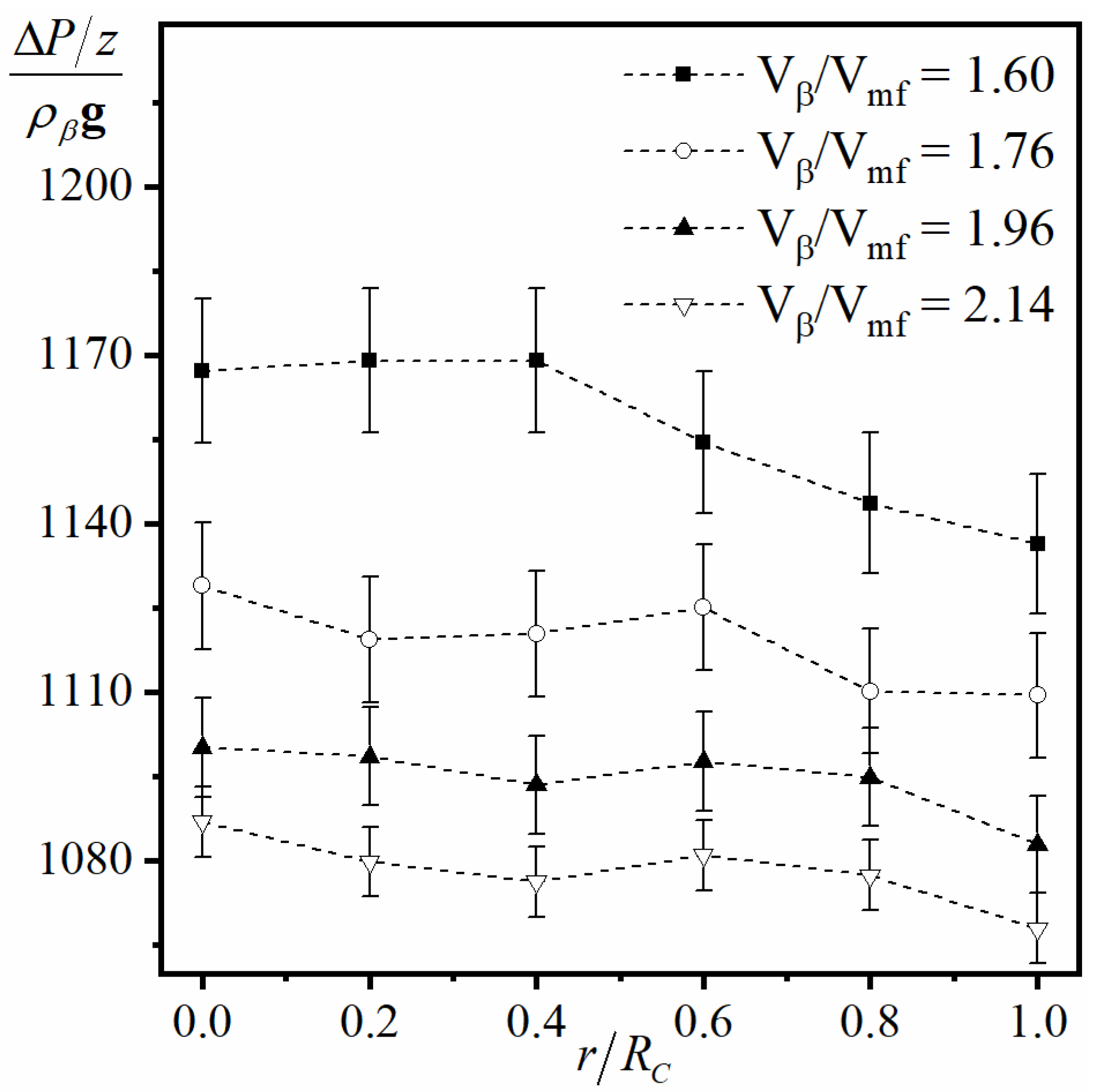
Figure 3 shows a sample of the obtained results by the DPTP for a fluidized bed packed with aluminum oxide particles. The results correspond to radial dimensionless pressure drop profiles $\left(\frac{\Delta P/z}{{\rho }_{\mathsf{\beta }}g}\right)$ in a fluidized bed column with an internal diameter of 0.14m, operating at different superficial inlet velocities, as studied and reported by Taofeeq and Al-Dahhan [26], where the error bars correspond to the standard deviation of the measurements. The DPTP can capture the radial differences in the pressure drop profiles. Remarkably, the pressure drop measured at the wall position $\left(r/R_{\mathrm{C}}=1\right)$ is always lower than the pressure measured at the other locations inside the bed, despite the radial variations being of a small-scale, especially when the superficial gas inlet velocity is increased. The radial variations can be attributed to the local variations of the flow fields, such as the difference in gas velocities crossing the probe head at the different radial locations.

The information obtained by this technique is essential for the local validation of mathematical models. However, it should be kept in mind that this is an invasive technique, and that there could be a disturbance in the hydrodynamics phenomena inside the fluidized bed due to insertion of the probe. Thus, to a certain extent, the observed trends in the measurements could also be affected by the measurement technique.

4.2. Two-Tip Optical Fiber Probe (TTOF)

The second developed technique for the measurement of local scale phenomena in fluidized beds and spouted beds are optical fiber sensors. Optical fiber sensors have been extensively used in experimental studies of gas–solid fluidized systems over the last decades [7,106,108,109]. Nevertheless, commonly, these sensors cannot simultaneously measure the solids holdup and velocities, show blind regions (their overall size is large and becomes highly invasive $\left(D_{\mathrm{probe}}\sim 2 \mathrm{cm}\right)$) or fail to provide accurate time resolved measurements [110,111,112]. As a response to these limitations of optical probes, in the mFReael, we developed a new Two-Tip Optical Fiber (TTOF) probe, which allowed simultaneous measurements of solids holdup and particles velocities, as well as other derived key hydrodynamic parameters, such as bubble rise velocity, bubble frequency and bubble chord length [20], along with a new simple and reliable calibration method for solids holdup and solids velocity [113].

Figure 4 shows a schematic diagram of the developed TTOF probe. This sensor consists of two sub-probes of 1 mm in diameter, which are fixed in a 3 mm in diameter probe, that keeps both sub-probes parallel and at a fixed distance of 1 mm from each other. When inserted into the system, the two sub-probes will remain vertically aligned, and hence, both sub-probes will measure relatively the same signal at slightly different times. An important difference with this probe, in comparison to other probes used in reported works in the literature, is that each of the sub-probes is composed of an alternating array of light emitting and receiving optical fibers of $15 \mathsf{\mu }\mathrm{m}$ in diameter. When the emitted light by the emitting optical fibers is reflected by the solid particles, it is sensed by the receiving fibers. The sensed back reflection of light is then transformed by a photomultiplier (also shown in Figure 4) into a voltage signal, which is then processed and captured in a personal computer. The calibration curve obtained by the new calibration method for solids holdup and solids velocity [113] is used to correlate the recorded voltage signal to the solids holdup.

The sampled data by both sub-probes is processed by a cross-correlation method, as described by Taofeeq et al. [113], to calculate the time shift $\left(\Delta t_i\right)$ between the two signals. Since both sub-probes are at a known distance of 1 mm, the instantaneous particle velocities $\left(v_{\mathsf{\sigma },i}\right)$ can be calculated according to Equation 35. The probe can capture whether the particles are moving upwards or downwards, which is indicated in the sign of the coefficient obtained by cross-correlation. With this information, particle velocity distributions at local positions inside the bed are obtained, and time-averaged particle velocity profiles can be estimated.

$$v_{\mathsf{\sigma },i}=\frac{1 \mathrm{mm}}{\Delta t_i}$$

(35)

$$v_{\mathrm{B},i}=\frac{1 \mathrm{mm}}{\Delta t_{\mathrm{B},i}}$$

(36)

Considering a similar cross-correlation processing of the sampled data by the sub-probes, and linking such processing with a bubble linking algorithm, as described by Rüdisüli et al. [114], a bubble linking time shift $\Delta t_{\mathrm{B},i}$ can be estimated. Modifying Equation (35) as indicated in Equation (36), a bubble rise velocity distribution and profiles can be obtained.

Further processing of the measured voltage signal allows us to estimate the bubble chord length and bubble frequency.

With this technique, the predictions of local solids holdup and solids velocity can be validated. Bubble-related parameters can also be validated for models that can predict these parameters, such as the model of Wang et al. [115], who implemented a PBM with a centralized coupling scheme to estimate bubble size distribution.

4.3. Dual Source γ-ray Computed Tomography (CT)

Despite the TTOF probe being able to measure pointwise information of the hydrodynamics phenomena inside gas-solid fluidized systems, it has the important limitation that the measurements are constrained to limited diameter locations inside the bed, and it is an invasive technique. As an alternative, our developed Dual Source γ-ray Computed Tomography (CT) is a non-invasive measurement technique that measures cross-section measurements. γ-ray CT is a radioisotope-based technique, that allows it to obtain time-averaged cross-sectional images of the phases’ distribution.

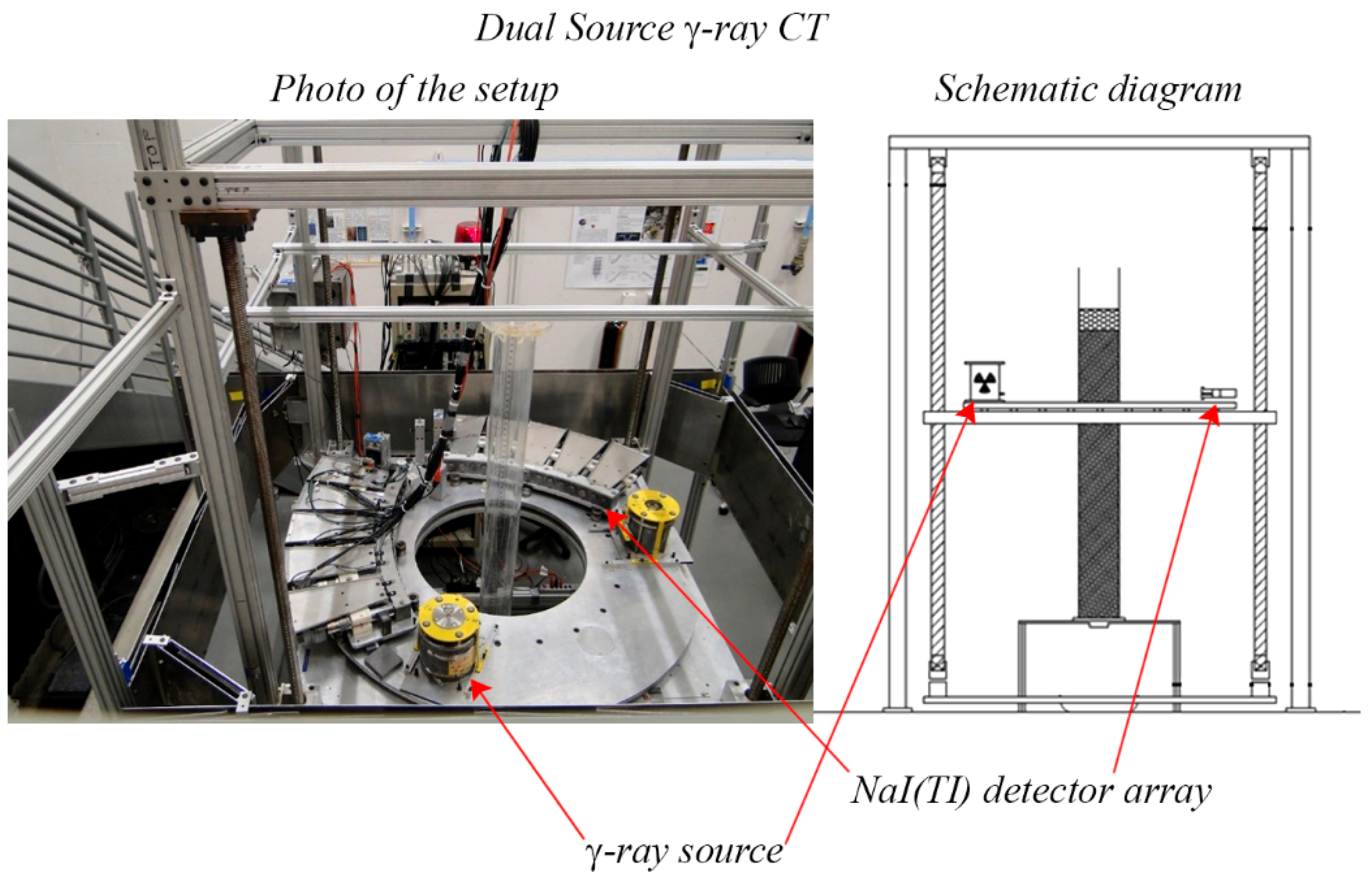
Our developed dual source γ-ray CT is composed two collimated γ-ray sources, a Cs-137 source and a Co-60 one. Each source is collimated with a horizontal 40° γ-ray beam of 5 mm in height. On the opposite side of each source, there is an arch array of 15 collimated Sodium Iodine (NaI(TI)) scintillation detectors, each of 2 inch in diameter. Each detector is covered by a lead collimator that provides a $5\times 2 \mathrm{mm}$ opening, in order to detect narrow γ-ray beams, and to enhance the spatial resolution and minimize the scattered γ-rays [116]. As shown in Figure 5, the sources and detectors are mounted on a horizontal rotary plate, which can also move in the axial direction.

In order to obtain a cross-sectional scan of the phases distribution, the sources and detectors array rotate 360° around the system places inside the γ-ray CT. The complete rotation around the system consists of 197 different positions of the source (views). At each view, the detectors array moves 21 different positions (projections). The recorded data by the 15 detectors adds to 65,055 data points $\left(197 \mathrm{views}\times 21 \mathrm{projections}\times 15 \mathrm{detectors}\right)$. This extensive full rotation scan takes around 6–8 h to be completed, with variations depending on the sample frequency and sample time [116]. The measurements are captured by a data acquisition system that consists of the 15 scintillation detectors, 30 timing filter amplifiers, 32 channel scalers, and a CC-USB CCAMAC controller.

The CT scans for gas-solid fluidized systems consist of three main steps [25,100,117]:

(1)

Scanning the empty column as a reference,

(2)

Scanning the column filled with the solid particles, without any gas flow, in order to measure the attenuation coefficient of the solid phase,

(3)

Scanning the column at operation conditions.

The collected data are processed by an Alternating Minimization (AM) algorithm [118], in order to obtain the attenuation values of each pixel of three cross-sectional images. The size of the images, and therefore the number and size of the pixels, depends on the size of the column placed in the CT and the width of the detector collimator. With the AM algorithm, the effective attenuation coefficient $\left({\widehat{\mu }}_{\mathsf{\sigma }-\mathsf{\beta }}\left(x\right)\right)$ at each pixel location $\left(x\right)$, as defined in Equation (37), is reconstructed.

$${\widehat{\mu }}_{\mathsf{\sigma }-\mathsf{\beta }}\left(x\right)={\widehat{\mu }}_{\mathsf{\sigma }}\left(x\right){\epsilon }_{\mathsf{\sigma }}\left(x\right)+{\widehat{\mu }}_{\mathsf{\beta }}\left(x\right){\epsilon }_{\mathsf{\beta }}\left(x\right)$$

(37)

In Equation (37), ${\widehat{\mu }}_{\mathsf{\sigma }}\left(x\right)$ and ${\widehat{\mu }}_{\mathsf{\beta }}\left(x\right)$ are the attenuation coefficients of the solid and phase, respectively. ${\widehat{\mu }}_{\mathsf{\beta }}\left(x\right)$ is reconstructed from step 1 mentioned above; ${\widehat{\mu }}_{\mathsf{\sigma }}\left(x\right)$ is reconstructed from step 2; and ${\widehat{\mu }}_{\mathsf{\sigma }-\mathsf{\beta }}\left(x\right)$ is reconstructed from step 3. ${\epsilon }_{\mathsf{\sigma }}\left(x\right)$ and ${\epsilon }_{\mathsf{\beta }}\left(x\right)$ are the solid and gas holdups at each pixel x, respectively.

Considering that in a gas–solid fluidized system, ${\widehat{\mu }}_{\mathsf{\sigma }}\left(x\right)\gg {\widehat{\mu }}_{\mathsf{\beta }}\left(x\right)$, Equation (37) can be simplified as shown in Equation (38). With this definition, the solid holdup at each pixel can be estimated according to Equation (39). The gas holdup can then be estimated recalling that ${\epsilon }_{\mathsf{\sigma }}+{\epsilon }_{\mathsf{\beta }}=1$, which is consistent with the definition of Equation (40).

$${\widehat{\mu }}_{\mathsf{\sigma }-\mathsf{\beta }}\left(x\right)\cong {\widehat{\mu }}_{\mathsf{\sigma }}\left(x\right){\epsilon }_{\mathsf{\sigma }}\left(x\right)$$

(38)

$${\epsilon }_{\mathsf{\sigma }}\left(x\right)=\frac{{\widehat{\mu }}_{\mathsf{\sigma }-\mathsf{\beta }}\left(x\right)}{{\widehat{\mu }}_{\mathsf{\sigma }}\left(x\right)}$$

(39)

$${\epsilon }_{\mathsf{\beta }}\left(x\right)=\frac{{\widehat{\mu }}_{\mathsf{\sigma }}\left(x\right)-{\widehat{\mu }}_{\mathsf{\sigma }-\mathsf{\beta }}\left(x\right)}{{\widehat{\mu }}_{\mathsf{\sigma }}\left(x\right)}$$

(40)

With this procedure, time-averaged cross-sectional solid and gas holdup distributions can be measured. This information allows us to locally validate the time-averaged predictions of models. The main limitation of the technique is that the scanning procedure takes a long time, which implies that in order to develop a large enough database for benchmarking of models, a rather lengthy experimental phase is needed. Furthermore, the technique cannot provide timewise measurements.

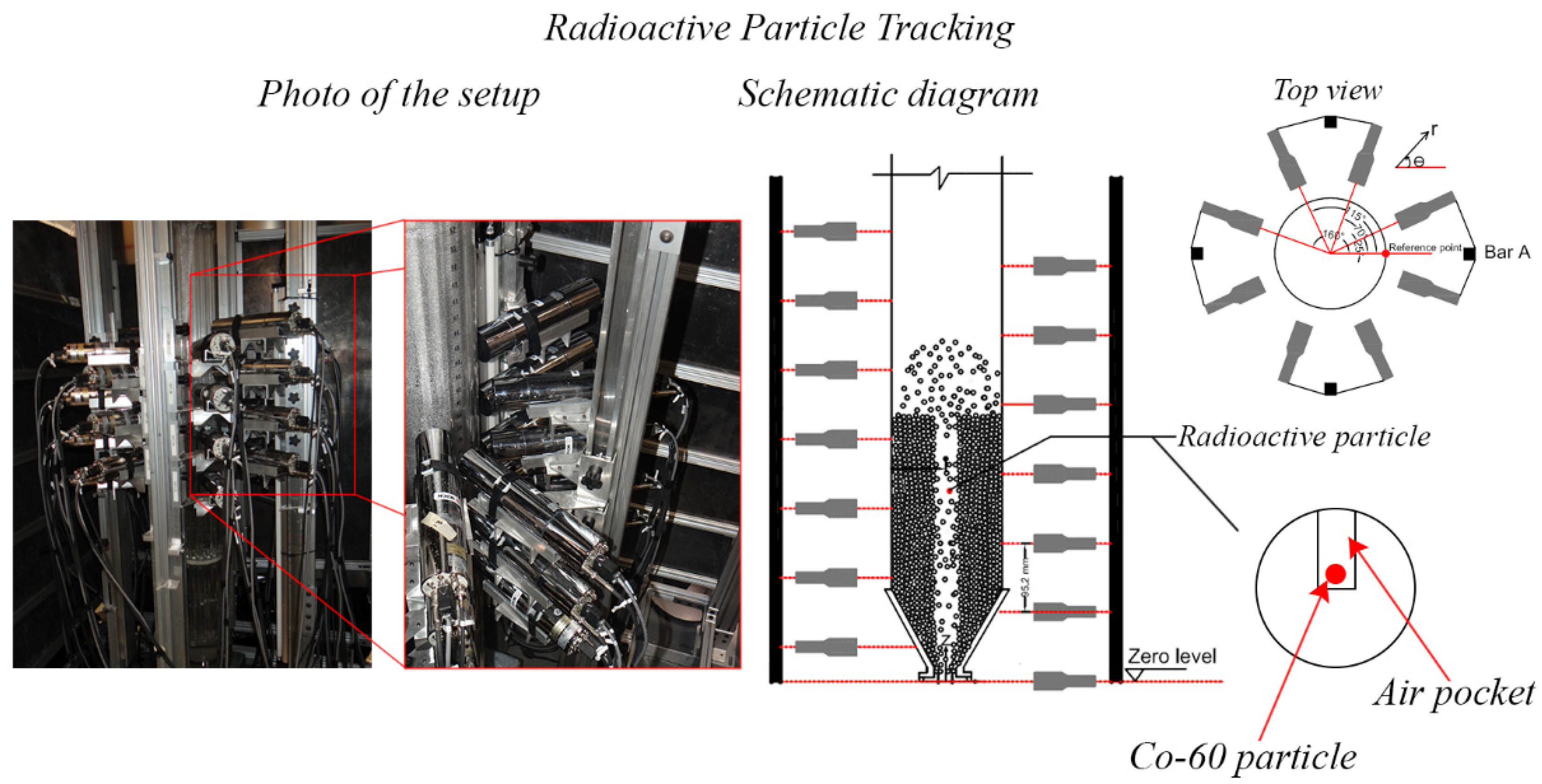
4.4. Radioactive Particle Tracking (RPT)

Another technique that allows us to obtain local scale non-invasive measurements in gas-solid fluidized systems is Radioactive Particle Tracking (RPT). In this technique, the motion of a single γ-ray emitting tracer particle, which mimics the solid phase, is followed. A set of detectors strategically placed around the system detects the radiation emitted by the particle, and the measurements allow us to determine the instantaneous position of the tracer and to reconstruct the lagrangian trajectory [16]. Despite this technique being present for the past few years [119,120,121], its application for fluidization had previously been a major challenge due to high velocities and high attenuation [100]. To overcome this challenge, our developed technique included a new fully automated calibration device and data acquisition and processing system [100].

The developed measurement technique, applied for both fluidized beds and spouted beds, uses a Cobalt-60 (Co-60) radioactive particle as tracer, which was irradiated at the University of Missouri Research Reactor Centre in Columbia, Missouri, USA. The Co-60 particle has a diameter of $600 \mathsf{\mu }\mathrm{m}$ and a density of $8900 \mathrm{kg}/{\mathrm{m}}^3$. In order to match the density of the solid phase, a hole is drilled in a ball of a different material, where the radioactive particle is encapsulated, and the size of the air pocket (size of the hole) is adjusted to match the required density. The material, size of the encapsulation and size of the air pocket, depends on the characteristics of the tracked phase. For example, Efhaima and Al-Dahhan [122] used a 1 mm in diameter aluminum ball to track the solid phase of a fluidized bed packed with Geldart B glass beads of $210 \mathsf{\mu }\mathrm{m}$ in diameter, while Al-Juwaya et al. [123] used a 2 mm in diameter stainless steel ball to track the steel packing in a spouted bed packed with a binary mixture of 2 mm glass beads and 2 mm steel shots, and for a different application, Sabri et al. [124] encapsulated the Co-60 particle in a 2 mm in diameter polypropylene ball to track the liquid phase in a split airlift photobioreactor for culturing microalgae. Detail of the encapsulation of the radioactive particle can be seen in Figure 6.

As shown in Figure 6, the RPT technique uses a set of Sodium Iodine (NaI(TI)) scintillation detectors strategically placed around the column. These detectors are similar to the ones used by the γ-ray CT, also of 2 inch in diameter, but without a collimator. The number and location of these detectors around the column will also depend on the studied system, with a maximum possible of 28 detectors. With an array of 28 detectors, Efhaima and Al-Dahhan [122] were able to obtain high-resolution measurements for a fluidized bed of 44 cm in diameter.

In order to determine the tracer particle position, a calibration step is required prior to each experimental condition tested. This calibration step consists of generating a map by placing the tracer particles at several known radial, angular and axial positions. At each of these known positions, the counts measured by each detector are recorded. This calibration step is fully automated by using an in-house developed device that places a calibration rod that holds the tracer particle at all the selected positions. The timewise positions of the particle in experimental conditions are reconstructed based on the count rate of each detector, by using the obtained calibration map along with a cross-correlation position algorithm, and a semi-empirical model to provide further calibration points. With the obtained particle position time series, the particle velocity vector can be calculated as shown in Equation (41).

$$\left(\begin{array}{c}{v}_{\mathsf{\sigma },r}\\ v_{\mathsf{\sigma },\theta }\\ v_{\mathsf{\sigma },z}\end{array}\right)=\frac{1}{t_{i+1}-t_i}\left(\begin{array}{c}{r}_{i+1}-r_i\\ \frac{r_{i+1}-r_i}{2}\left({\theta }_{i+1}-{\theta }_i\right)\\ z_{i+1}-z_i\end{array}\right)$$

(41)

With the velocity vectors obtained by Equation (41), further processing allows us to obtain cross-sectional average velocity profiles, as well as velocity fluctuations, turbulent stresses and turbulent kinetic energy per unit mass.

This technique, as well as the TTOF probe, allows us to locally validate the velocity profiles predictions of the implemented models. RPT has the advantage of being non-invasive, in comparison with the TTOF probe technique. However, implementing RPT on a system requires long preparation times, as a calibration step is required to be conducted at each of the tested experimental conditions. Moreover, RPT experiments have to be run for prolonged times (~6 h) in order to allow the tracer particle to visit every location inside the bed, in order to obtain reliable and useful information.

5. Pairing Experimental and Mathematical Modelling Studies

In an attempt to enhance the quality of the predictions of local hydrodynamic fields on gas-solid fluidization, we implemented a simplified E2P model based on the bed elasticity approach. In this model, the governing equations for the gas phase were set to be described by Equations (3), (4) and (7), while the governing equations for the solid phase, considering the discussion on Section 3, incorporated the continuity equation described in Equation (5), and the momentum balance defined as follows:

$${\epsilon }_{\mathsf{\sigma }}{\rho }_{\mathsf{\sigma }}\left[\frac{\partial v_{\mathsf{\sigma }}}{\partial t}+v_{\mathsf{\sigma }}\cdot \nabla v_{\mathsf{\sigma }}\right]=-{\epsilon }_{\mathsf{\sigma }}\nabla P-G\left({\epsilon }_{\mathsf{\beta }}\right)\nabla {\epsilon }_{\mathsf{\beta }}+{\epsilon }_{\mathsf{\sigma }}\nabla \cdot \left[{\mu }_{\mathrm{eff}}\left(\nabla v_{\mathsf{\sigma }}+{\left(\nabla v_{\mathsf{\sigma }}\right)}^T\right)\right]+{\epsilon }_{\mathsf{\sigma }}{\rho }_{\mathsf{\sigma }}g-F_{\mathrm{d}}$$

(42)

where ${\mu }_{\mathrm{eff}}$ was defined according to Equation (27), by virtue of its simplicity and the shown evidence of providing an adequate scale estimate for an effective pseudo-phase viscosity. $F_{\mathrm{d}}$ was selected to follow Gidaspow’s sub-model [73], which defines the multiphase interaction coefficient $\left(K_{\mathsf{\sigma }\mathsf{\beta }}\right)$, as per Equations (29)–(31), since this model has been widely practically validated in the literature [12,53,62,83,84,85].

Regarding the selection of the modulus of elasticity sub-model $\left(-G\left({\epsilon }_{\mathsf{\beta }}\right)\right)$, all the sub-models found to be reported in the literature were developed on early contributions of numerical studies of fluidization, with some of the models being over 50 years old. The developed sub-models were constrained to the available measurement techniques of the moment, resulting in sub-models based on macroscopic measurements, with no regard of the local-scale phenomena. Considering this important limitation, the major challenge in the implemented approach was to define an insightful modulus of elasticity sub-model that could predict the local scale phenomena on a fluidized bed.

As shown in Table 1, there are vast options of sub-models that can be selected to model the modulus of elasticity on fluidized beds. In a modeling environment where diverse alternatives could be considered, it is important to discern between the options based on the underlying assumptions for the derivation of each model. In this sense, there is also a need to recognize the main characteristics of the experimental system to model.

Several moduli of elasticity sub-models were tested in order to observe the local predictive quality of the overall model, and the sensitivity to these changes. Nevertheless, the selection of the sub-models should be made in accordance with the derivation of the models, their assumptions and their applicability range. In this sense, the modulus of the elasticity sub-model proposed by Ettehadieh and Gidaspow [67] should be highlighted. This model was developed for fine particles, based on the experimental results of Mutsers and Rietma [66]. The experimental study to obtain the data for the development of such sub-models was obtained from an experimental tilting bed apparatus [68]. The tilting bed apparatus was a separate-effect experimental setup to determine interparticle forces, which consisted of a bench-scale fluidized bed, where fine solid particles were expanded without reaching bubbling. Once steadily expanded, the whole bed slowly tilted, and the tilt angle was obtained until the surface of the bed remaining undisturbed was recorded. The experimental observations of such tilt angles at different bed expansions were indicative of the interparticle forces. One important remark of their findings was that the interparticle forces, and therefore the modulus of elasticity, did not seem to depend on the mean particle diameter, but it exhibits important variations when there is a large particle size distribution, such as in the case where fines are present. Considering the fluidized bed experimental setups modeled, which consisted of fluidized beds without internals, packed with Geldart B particles, and where a large particle size distribution was not observed, the sub-model of Ettehadieh and Gidaspow [67], as shown in Table 1, seems to be adequate for modeling the modulus of elasticity in these systems.

Some of the tested sub-models did not converge, such as when using the sub-model proposed by Uribe et al. [49], which was expected, as this model was developed for a spouted bed. Among the modulus of elasticity tested, Figure 7 compares the sub-models that led to the most accurate predictions of the local fields. Figure 7 shows the locally predicted solid holdup of the model by using an Ettehadieh and Gidaspow sub-model and other sub-models listed in Table 1, for a sample case of the fluidized bed reported by Taofeeq et al. [20,26,125]. In this figure, the error bars on the experimental data correspond to the standard deviation of the measurements. At each radial location, measurements were taken for 65 s, with a frequency of 5 Hz, and were repeated 5 times. The modulus of elasticity proposed by Ettehadieh and Gidaspow leads to accurate radial solid holdup profiles.

Table 4. Average Absolute Relative Error (%) in the time-averaged predicted radial solids holdup profiles for for a fluidized bed of $D_{\mathrm{C}}=14 \mathrm{cm}$, operating at ${\langle V_{\mathsf{\beta }}\rangle }_0/V_{\mathrm{mf}}=1.60$, using different modulus of elasticity sub-models.

	Sub-Model
$\mathit{z}/{\mathit{D}}_{\mathbf{C}}$	Ettehadieh and Gidaspow [67]	Gidaspow [73]	Kuipers et al. [74]
0.75	4.5	8.8	6.9
1.45	13.9	12.5	17.4
2.0	10.8	12.1	12.6
$\langle AARE\rangle$	9.76	11.5	12.3
$\langle AARE\rangle =\frac{1}{n_j}{\displaystyle \sum _j\left(AAR{E}_j\right)}$

shows a comparison of the Average Absolute Relative Error $\left(AARE={\displaystyle {\sum }_{i=1}^n\left(\left|{\psi }_{\mathrm{EXP},i}-{\psi }_{\mathrm{Model},i}\right|/{\psi }_{\mathrm{EXP},i}\right)/n}\right)$ obtained in the predicted profiles shown in Figure 7. Similar deviations in the predictions for other operation conditions were observed, and the model of Ettehadieh and Gidaspow always exhibited a similar predictive quality. Thus, according to these results, $-G\left({\epsilon }_{\mathsf{\beta }}\right)$ in Equation (42) was defined for the fluidized bed model as per Ettehadieh and Gidaspow, which was expected according to the previous discussion. Nevertheless, it should be taken into account that the implemented sub-model is also tied to the previously discussed limitations of the modulus of elasticity, meaning that this model was developed based on overall measurements of a simplified experimental apparatus. An improvement in the local predictions could be obtained by the development of a new modulus of elasticity sub-model based on local scale measurements.

5.1. Experimental Setup

Two experimental systems were considered. The first one, reported by Taofeeq et al. [20,26,125], consists of a fluidized bed of a diameter of $D_{\mathrm{C}}=14 \mathrm{cm}$, and a height of $L_{\mathrm{C}}=184 \mathrm{cm}$. The column was packed to a static bed height of $L_{\mathsf{\sigma },0}=35 \mathrm{cm}$ with Geldart B type glass beads, which had an average particle diameter of $\langle D_{\mathsf{\sigma }}\rangle =365 \mathsf{\mu }\mathrm{m}$, with a minimum particle diameter of around $D_{\mathsf{\sigma },\min }=300 \mathsf{\mu }\mathrm{m}$, and a density of ${\rho }_{\mathsf{\sigma }}=2500 \mathrm{kg}/{\mathrm{m}}^3$. The fluidized bed was operated at relative gas inlet velocities between ${\langle V_{\mathsf{\beta }}\rangle }_0/V_{\mathrm{mf}}=1.6-1.96$. This system was studied by Taofeeq et al. by using TTOF probes and DPTP, which allowed us to determine radial solids velocity, holdup and pressure drop local profiles.

The second system has been reported by Efhaima and Al-Dahhan [100,122], and also consists of a fluidized bed packed with Geldart B type glass bead particles. The difference is that this system had a diameter of $D_{\mathrm{C}}=44 \mathrm{cm}$, height of $L_{\mathrm{C}}=487 \mathrm{cm}$, static bed height of $L_{\mathsf{\sigma },0}=88 \mathrm{cm}$, and the solid particles had an average diameter of $\langle D_{\mathsf{\sigma }}\rangle =210 \mathsf{\mu }\mathrm{m}$. by Efhaima and Al-Dahhan implemented γ-ray CT and RPT to determine in a non-invasive way the solid holdup and velocity cross-sectional profiles.

Considering these two systems will allow us to assess the local predictive quality of the implemented model, as well as to assess the scale dependency of the model.

5.2. Results: Comparison with Experiments

A model for fluidized beds with the characteristics discussed above had been available in the literature for decades. However, important limitations in the available computational resources resulted in models considering a 2D computational domain, or considering further simplifications and assumptions to reduce the complexity of the model [71]. Furthermore, no local validation of the predicted profiles had been reported. Implementing the model discussed above, in a previous contribution, we conducted a study to locally validate the model [53]. The model incorporated important differences in comparison with similar models reported in the literature, such as considering the 3D computational domain, and no further simplifications on the transport equations.

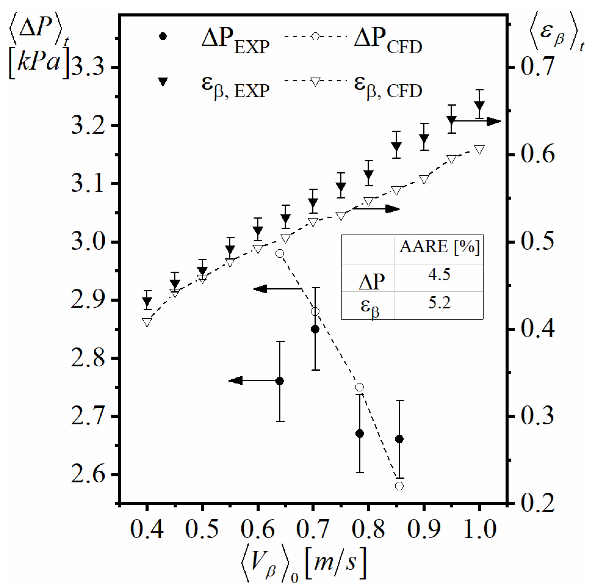
As shown in Figure 8, first a validation of the macroscopic parameters predictions was conducted by comparing the time averaged overall gas holdup $\left({\langle {\epsilon }_{\mathsf{\beta }}\rangle }_t\right)$ and the time averaged overall pressure drop $\left({\langle \Delta P\rangle }_t\right)$. In this figure, the error bars represent the standard deviation of the measurements, as reported by Taofeeq et al. [20,26,125] The model with the discussed characteristics had a high accuracy in the prediction of these two important macroscopic parameters. The model predicted these parameters with an AARE of 4.5% and 5.2% for ${\langle \Delta P\rangle }_t$ and ${\langle {\epsilon }_{\mathsf{\beta }}\rangle }_t$, respectively.

Nevertheless, the prediction of overall parameters is not insightful of the predictive quality of the model for the local scale phenomena. Furthermore, the experimental measurements of macroscopic parameters relies on overall observations, overlooking the behaviors inside the bed. The limitation of this is clearly identified when determining overall time averaged solids holdup. Usually, this macroscopic parameter is experimentally determined by comparing the dynamic bed height at a certain operational condition against the static bed height [96].

Table 5. Average Absolute Relative Error (%) in the overall parameters prediction for a fluidized bed of $D_{\mathrm{C}}=14 \mathrm{cm}$, operating at ${\langle V_{\mathsf{\beta }}\rangle }_0/V_{\mathrm{mf}}=1.60$, using different modulus of elasticity sub-models.

		Sub-Model
Parameter	Experimental	Ettehadieh and Gidaspow [67]	Gidaspow [73]	Kuipers et al. [74]
${\langle \Delta P\rangle }_t\left[\mathrm{kPa}\right]$	2.75	2.96	3.09	3.10
$\langle AARE\rangle \mathrm{of} {\langle \Delta P\rangle }_t$		7.6%	12.4%	12.7
${\langle {\epsilon }_{\mathsf{\sigma }}\rangle }_t$	0.52	0.49	0.51	0.52
$\langle AARE\rangle \mathrm{of} {\langle {\epsilon }_{\sigma }\rangle }_t$		7.3%	3.5%	1.6%

compares the predicted overall pressure drop and overall solid holdup predicted by the model using a different modulus of elasticity sub-models, for the sample case shown in Figure 7 and Table 4. Comparing these overall predictions, these three sub-models lead to a model with a similar predictive quality. In fact, it seems that the models that couples the Kuipers et al. sub-model can better predict the solid holdup. However, as shown in Figure 7, the model that leads to the most accurate predictions of the local solid holdup profile is the one that couples Ettehadieh and Gidaspow sub-model.

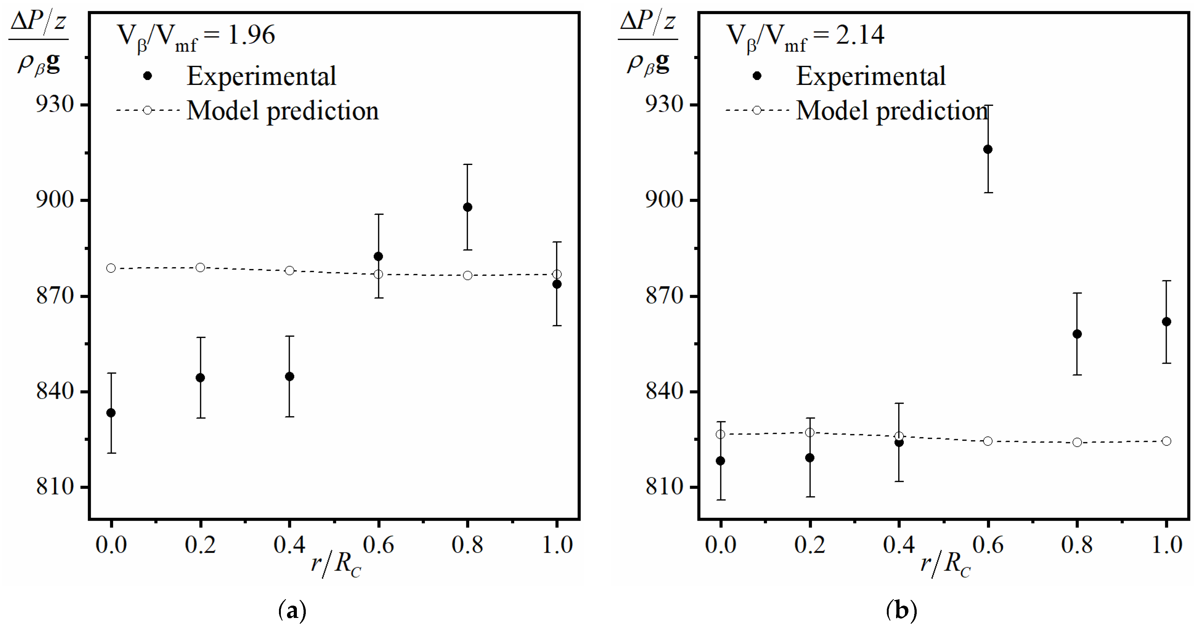
Figure 9a,b shows a sample of the comparison between the predicted pressure drop profile and the experimentally determined local pressure drop profile by using the DPTP technique, as reported by Taofeeq and Al-Dahhan [26], for the fluidized bed of $D_{\mathrm{C}}=14 \mathrm{cm}$. Error bars represent the standard deviation of the measurements. According to the previous observations, the predictions shown corresponds with the model that couples Ettehadieh and Gidaspow sub-model. It can be seen that the model is able to predict the values and trends of the experimentally determined profiles. However, it should be noted that the experimental measurements exhibit high variations of the profiles, especially in the region close to the wall. This source of deviation in comparison with the model predictions can be attributed to systematic errors in the measurement technique, or to unquantified wall effects in the experimental measurements that affect the DPTP measurements in the near-wall regions. Despite such deviations, the AARE for these cases was found to be 2.8% and 3.4% for ${\langle V_{\mathsf{\beta }}\rangle }_0/V_{\mathrm{mf}}=1.96$ and ${\langle V_{\mathsf{\beta }}\rangle }_0/V_{\mathrm{mf}}=2.14$, respectively. A similar predictive quality was observed for all other tested cases. This suggests that the implemented model can predict the overall and local pressure drops with a high accuracy.

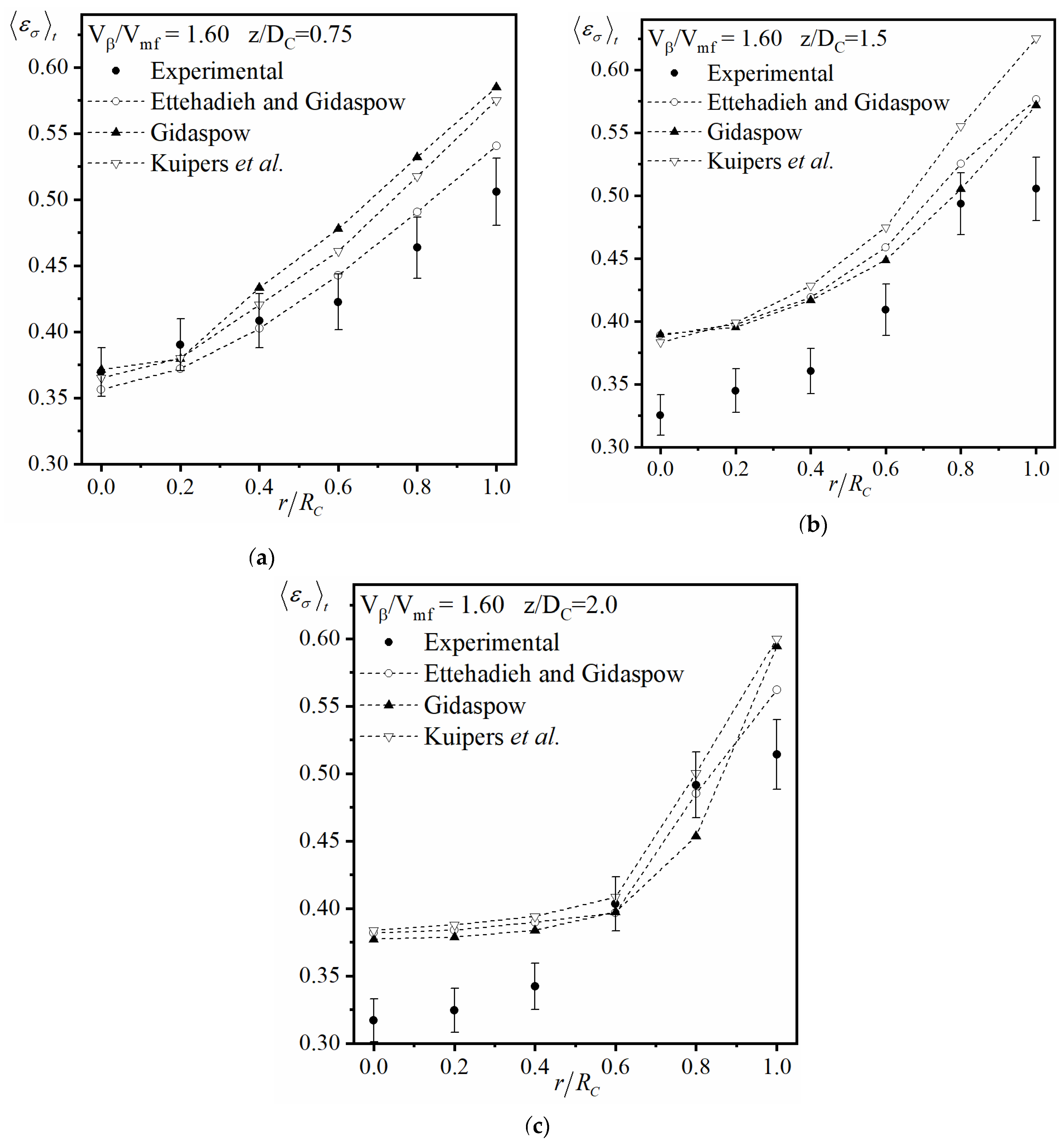
Similarly, Figure 10a,b shows a sample of the comparison of experimentally determined and model-predicted solid holdup profiles for the fluidized bed of $D_{\mathrm{C}}=14 \mathrm{cm}$, at an axial location of $z/D_{\mathrm{C}}=0.75$. The experimental data on these figures were obtained by the TTOF probe, which implies that the data were obtained at discrete locations by an invasive technique. In this figure, the error bars also represent the standard deviation of the measurements. The observed deviations between measurements and predicted profiles can be attributed to these limitations of the technique. Despite this, it can be seen that the model properly predicts the solids holdup profile values and trends, with an AARE of 4.5% and 7.6% for ${\langle V_{\mathsf{\beta }}\rangle }_0/V_{\mathrm{mf}}=1.60$ and ${\langle V_{\mathsf{\beta }}\rangle }_0/V_{\mathrm{mf}}=1.76$, respectively. Again, for other operation conditions, the predictive quality remained similar. This also suggests a high local accuracy of the implemented model.

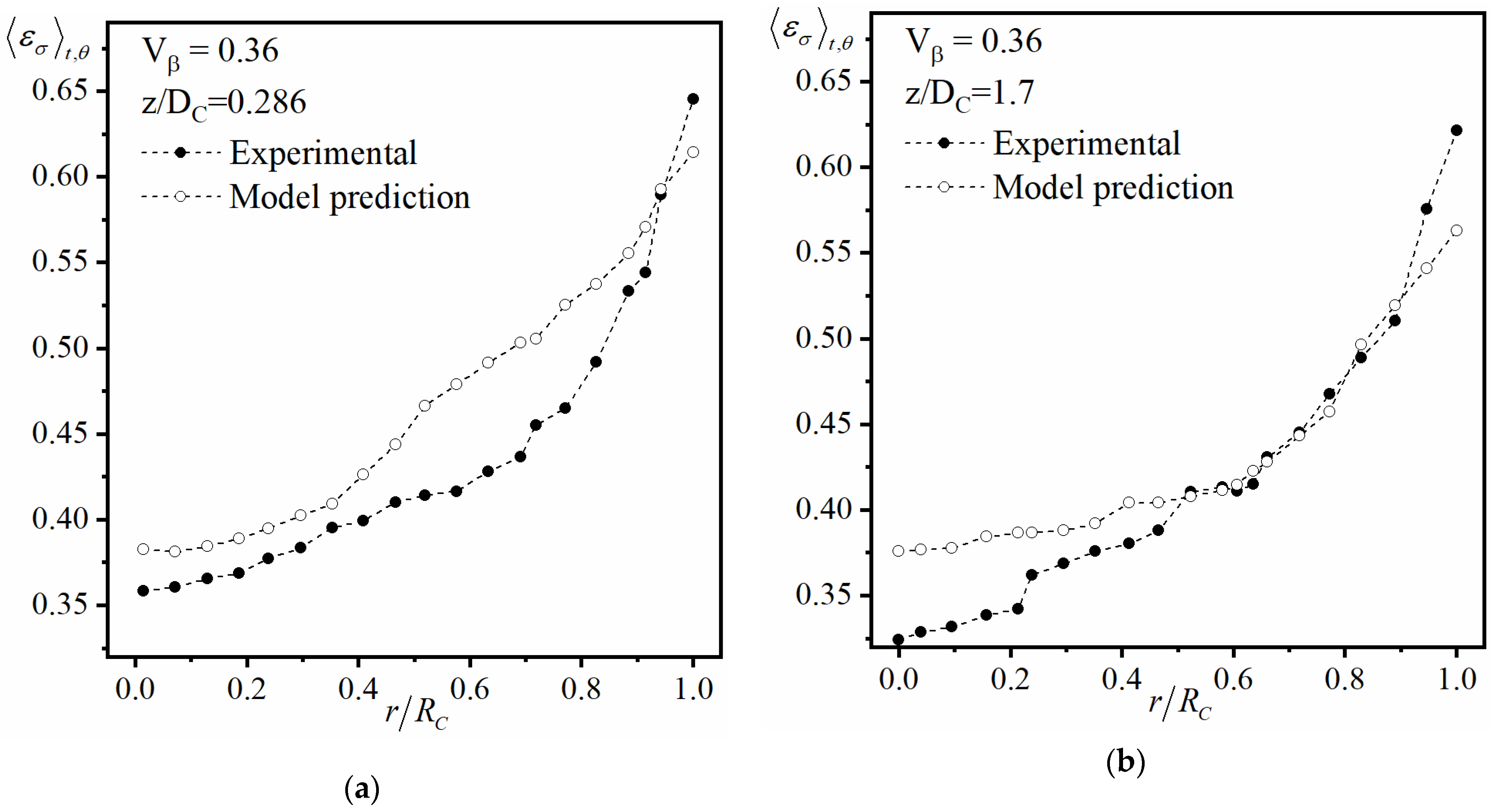
A more detailed local validation of the local holdup profile can be observed in Figure 11a,b. In these, a comparison of the time and azimuthally averaged solids holdup profile can be observed for the fluidized bed case of $D_{\mathrm{C}}=44 \mathrm{cm}$, as reported by Efhaima and Al-Dahhan [100,122]. In these, the experimental data were obtained by using γ-ray CT, where the cross-sectional scan results were azimuthally averaged. It can be seen that the time and azimuthally averaged solid holdup profiles show more details of the solids distribution inside the bed, since the full non-symmetrical chaotic behavior expected on fluidized beds is captured. It can be seen that the model is also able to predict these trends and values. The deviations in the predictions can be attributed to the fact that the γ-ray CT could have limitations in capturing the behaviors in the central regions of the bed, since the fluidized bed system is a highly attenuating media, due to the density of the packing and the large column diameter. Despite this, the model was able to predict these profiles with an AARE of 7.8% and 5.9% for the cases of $z/D_{\mathrm{C}}=0.286$ and $z/D_{\mathrm{C}}=1.7$, respectively. It is also remarkable to observe that the predictive quality of the model and coupled sub-models seem to be scale independent, as the predictions were accurate for both fluidized beds of different scales.

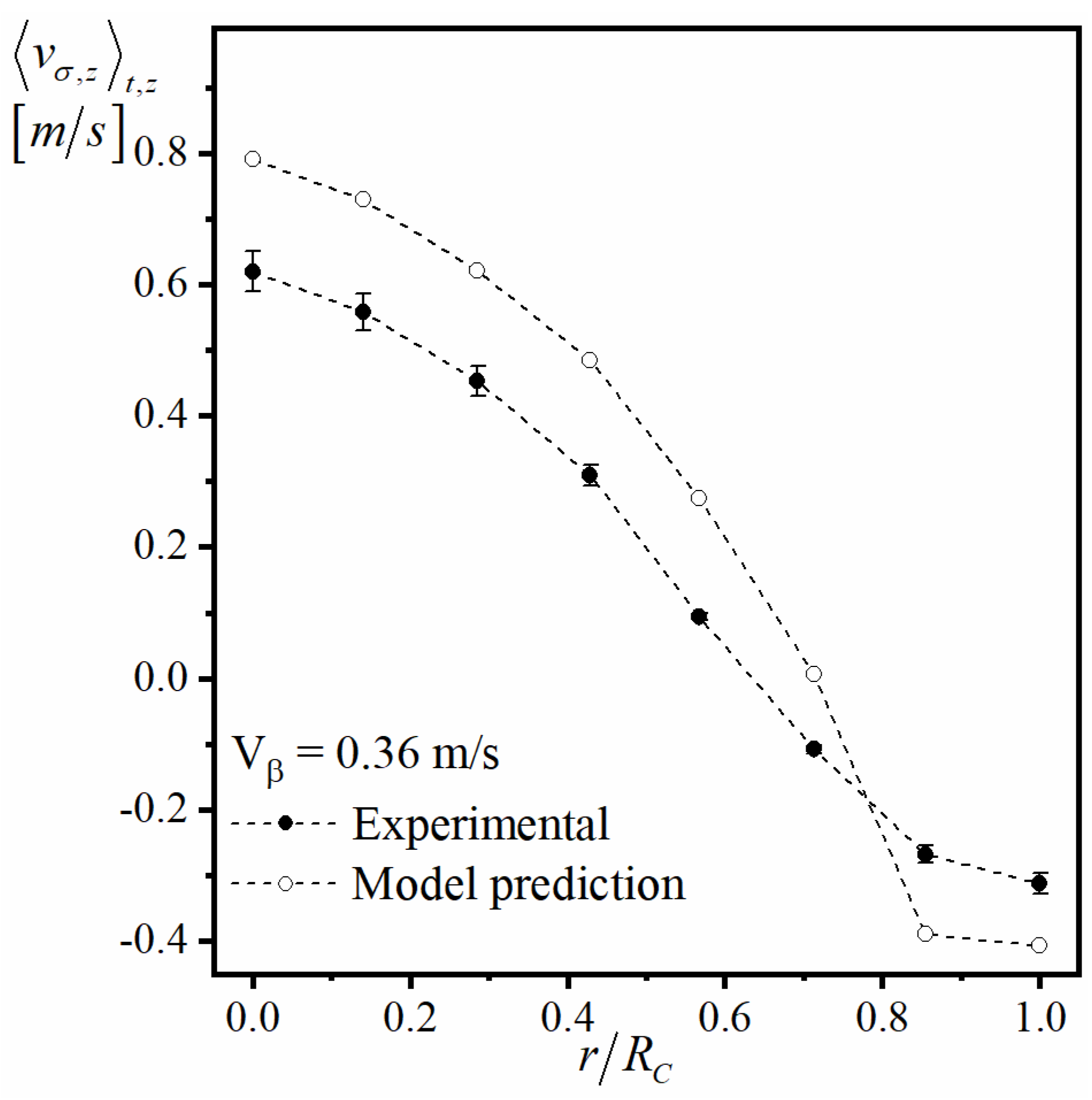
Similarly, Figure 12 shows a comparison of the experimentally determined and predicted azimuthally and axially averaged axial solids velocity profile on the fluidized bed reported by reported by Efhaima and Al-Dahhan [100,122]. The experimental results were obtained by using RPT, averaging the axial component of the solid velocity vector described in Equation (41) axially and azimuthally. A similar averaging procedure was done in the model predictions for comparison purposes. It can be seen that the model can also properly capture the solids velocity values and trends, and properly predicts the recirculation zones. The solids velocity profile shown in Figure 12 was predicted with a Mean Squared Deviation $\left(MSD=\frac{1}{n_i}{\displaystyle \sum _i{\left[{\left({\psi }_{\mathrm{Model}}\right)}_i-{\left({\psi }_{\mathrm{EXP}}\right)}_i\right]}^2}\right)$ of $0.023 \mathrm{m}/\mathrm{s}$. Similar predictions were obtained at other operation conditions.

The highest deviations in the predictions of the local phenomena is observed in the predictions of solids velocities. This was also observed when comparing the model predictions against solids velocities determined by a TTOF probe [53]. These deviations can be attributed to the underlying limitation of the coupled modulus of the elasticity sub-model. Hence, in order to improve the predictions of the local solids velocity, a new and improved modulus of elasticity, developed considering the local scale information, is needed.

Implementing the Euler-Euler with a bed elasticity approach for the fluidized bed case required merely a proper selection of the coupled sub-models. In this sense, pairing the mathematical modeling study with the advanced experimental study allowed to obtain insights into the level of detail in the modeling required to obtain a locally predictive model. Remarkably, the model with such simplified characteristics, such as a reduced number of coupled sub-models, was able to predict with high accuracy, the key local hydrodynamic parameters. As suggested by Al-Dahhan et al. [17,99,109,126,127], the hydrodynamic parameters predicted by the implemented model are of paramount importance for scale-up tasks. Specifically, Al-Dahhan et al. have demonstrated that two fluidized beds of different scales will exhibit a similar hydrodynamic behavior when the local solids holdup profiles are matched in both systems. Hence, the implemented model, can be useful for assessing local hydrodynamic behavior of fluidized beds of different scales, and can aid in scale-up tasks. The model, however, is not able to predict other parameters, which could be of importance for other tasks, such as bubble size distribution, and cluster size distribution.

6. Remarks

Modeling gas-solid fluidized systems is still a major challenge, and further research efforts are required in the years to come. The current status of modeling these systems has focused on the addition of further sub-models to account for multiphase and multiscale phenomena. However, such practice has led to models that couple a vast number of sub-models and rely on a vast number of closure and fitting parameters. Models with these vast coupling of sub-models become virtually impossible to optimize due to the vast sources of uncertainties in them. Hence, a simplified approach that can provide accurate local predictions of the multiphase flow phenomena fields is required.

In order to explore a possible alternative, we proposed modifying and implementing an underexplored approach for gas-solid fluidized systems based on the so-called bed elasticity approximation. In order to implement such a model, detailed and reliable experimental information of local fields is necessary. In this sense, recent advances in invasive and non-invasive measurement techniques become of primal importance. Remarkably, four of our in-house techniques can provide such a level of detail needed for benchmarking of the implemented models: (i) Differential Pressure Transducer Probe (DPTP), (ii) Two-Tip Optical Fiber probe (TTOF), (iii) Dual Source γ-ray Computed Tomography (CT), and (iv) Radioactive Particle Tracking (RPT).

It was observed that pairing the results obtained by these advanced measurement techniques allowed us to develop and implement highly predictive models for fluidized beds. The bed elasticity approach had been underexplored in the literature, and no models using this approximation had been locally validated. In this work, it was noted that this approach could lead to the accurate local prediction of the key hydrodynamic parameters, such as pressure drops, solids holdup and solids velocity. Furthermore, such a simplified approach has a high adaptability, and could be modified to provide accurate predictions of local fields on other gas–solid fluidized systems, such as spouted beds. In order to enhance the predictive quality of the implemented model, a new modulus of the elasticity sub-model can be developed based on the local scale information obtained by advanced measurement techniques. Forthcoming research efforts will be focused on the development of such an enhanced model.