Modelling Sessile Droplet Profile Using Asymmetrical Ellipses

Abstract

Modelling the profile of a liquid droplet has been a mainstream technique for researchers to study the physical properties of a liquid. This study proposes a facile modelling approach using an elliptic model to generate the profile of sessile droplets, with MATLAB as the simulation environment. The concept of the elliptic method is simple and easy to use. Only three specific points on the droplet are needed to generate the complete theoretical droplet profile along with its critical parameters such as volume, surface area, height, and contact radius. In addition, we introduced fitting coefficients to accurately determine the contact angle and surface tension of a droplet. Droplet volumes ranging from 1 to 300 µL were chosen for this investigation, with contact angles ranging from 90° to 180°. Our proposed method was also applied to images of actual water droplets with good results. This study demonstrates that the elliptic method is in excellent agreement with the Young–Laplace equation and can be used for rapid and accurate approximation of liquid droplet profiles to determine the surface tension and contact angle.

1. Introduction

The behaviour and properties of a liquid droplet have long been an attractive research topic. Researchers have been able to study both static and dynamic behaviours of liquid droplets such as mobility on a solid surface, evaporation, or coalescence by analysing critical droplet parameters. Throughout the past two centuries, researchers have focused on studying droplet shapes as a critical parameter [1,2,3]. Droplet shapes are governed by the capillary length of the liquid and surface energy of the solid substrate on which the droplet rests on. Depending on the droplet volume, its shape varies from a spheroid (<10 µL) to a puddle (>100 µL). The two most commonly used methods to study droplet shapes are (i) the sessile drop method, where a droplet rests on a horizontal solid substrate, and (ii) the pendant drop method, where a droplet is suspended from the tip of a needle. In the pendant drop method, the surface tension is determined through droplet shape analysis [4,5]. On the other hand, the scope of measurements is wider for the sessile drop method where the surface tension, contact angle, and surface free energy of the solid surface are generated from the analysis due to interactions between the droplet and solid substrate. This information is used to determine the wettability of a surface, which is essential for many fields including coating, inkjet printing, and digital microfluidics, as well as biological and chemical processes [6,7,8,9].

A hypothetical droplet profile is constructed by fitting a series of data points based on a suitable mathematical model. Various parameters have been thoroughly studied using the generated data points of hypothetical droplet profiles. Currently, a variety of curve-fitting solutions for droplet modelling exist either as separate tools or as integral parts of a droplet measurement technique. Simple geometrical models such as the spherical method or the conic section method are mainly used for droplets with a small volume and a limited range of contact angles (0–100°) [10,11], whereas the Young–Laplace equation is universally applied since it is derived from fluid physics. Numerically solving the Young–Laplace equation generates an ideal droplet which corresponds to a real sessile droplet resting on a smooth solid surface. Solutions to the Young–Laplace equation have been proposed, with some notable works on the generation of tables of parameters relating to different droplet shape factors [12] using the minimisation of energy to obtain the governing differential equation for the shape of the droplet [13,14,15], or by applying the fourth-order Runge–Kutta method as a numerical solution to examine axisymmetric droplet interfaces [16]. Axisymmetric droplet shape analysis (ADSA) is a powerful droplet analysis technique developed based on the Young–Laplace equation. Throughout the years, different versions of the ADSA method have been developed such as ADSA—Profile [17,18], ADSA—Diameter (ADSA–D) [19], and ADSA—Height and Diameter (ADSA–HD) [20]. Besides measuring conventional liquid droplets, these tools have been used to analyse liquid marbles, which are liquid droplets coated with micro- or nanoparticles [21,22,23,24,25,26,27]. Thanks to their unique features such as high elasticity, self-propulsion, and ability to coalesce, liquid marbles are present in applications such as micro- or nanoscale chemical reaction control, microfluidics, or cosmetics [28,29,30,31,32,33,34,35,36,37,38,39,40,41]. When liquid marbles rest on a flat and smooth surface, they are analogous to a sessile droplet on a non-wetting solid surface [42]. Therefore, the shape of liquid marbles upon interaction with a liquid or solid substrate can be investigated via modelling techniques catered for conventional liquid droplets.

Modern droplet modelling tools are extremely versatile and highly effective in terms of producing and analysing liquid droplets [43,44,45,46]. However, highly precise instruments packaged with proprietary analysis software tend to cost tens of thousands of dollars. Thus, the development of a cost-effective and easily accessible alternative modelling technique will facilitate the research of sessile droplets in various settings. This study proposes an elliptic model to generate sessile droplet profiles which provide measurable parameters such as contact angles and surface tensions. This model divides the droplet into two elliptic curves which can be uniquely defined using an analytical method. The model accurately generates the surface tension of the liquid using only two points from the top half of the droplet. Moreover, if the position of the three-phase contact point is known, the model can generate the contact angle which is difficult to measure accurately. Our elliptic model generates all these critical parameters without iteration which eliminates the need for complex algorithm optimisation.

2. Theoretical Background

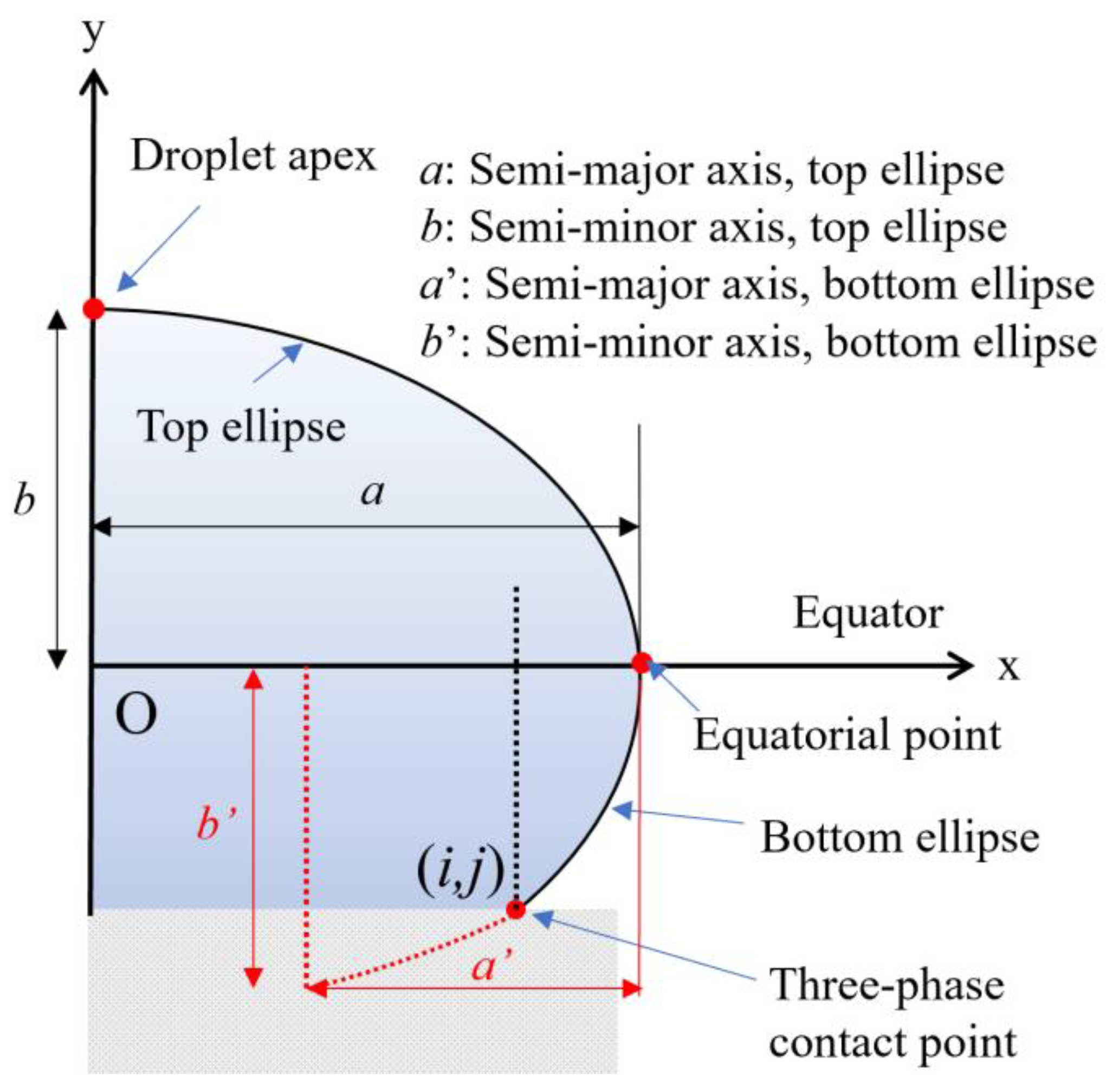
The profile of a sessile droplet can be approximated as a truncated circle. However, this approximation only applies to extremely small droplets. For larger droplets, the profile can be estimated as a truncated ellipse instead. This approximation applies to droplets with contact angles less than 90°. For larger contact angles, the bottom portion of the droplet no longer conforms with the elliptic curve. This study accurately models the profiles using distinct top and bottom half ellipses. The asymmetric ellipses are bordered by a shared equator where the droplet width is at its maximum.

2.1. Defining the Ellipses

First, we split the droplet into the top and bottom ellipses, Figure 1. The origin of the coordinate system is defined as the intersection between the equator and the vertical axis of symmetry. The general equation for an ellipse can be formulated as

$$\frac{{\left(x-x_0\right)}^2}{a^2}+\frac{{(y-y_0)}^2}{b^2}=1$$

(1)

where a and b are the semi-major and semi-minor axes, respectively; x and y are represented as standard parametric equations such that x = a cos t and y = b sin t, where t is an angle that ranges from 0 to 90°. The top ellipse is centred at the origin (0,0) such that x₀ = y₀ = 0. For the bottom ellipse, the semi-major and semi-minor axes are defined as a′ and b′. The bottom ellipse is centred at (a−a′,0) instead of the origin such that both the top and bottom ellipses share the same equatorial point.

The respective ellipses were defined using image analysis on a captured digital image of a real droplet to determine the coordinates of three critical points. The critical points are the top point, the equatorial point, and the bottom point, which is the three-phase contact point, Figure 1.

The interp1 command in MATLAB was used to generate the interpolated function f as the elliptical curve. By revolving the elliptical curve f around the vertical axis, we obtained the volume and surface area of the ellipses. Therefore, the volume V and surface area S can be written as

$$V=\pi {\displaystyle {\int }_j^b}{f}^{2}dy$$

(2)

$$S=2\pi {\displaystyle {\int }_j^b}\left|f\right|\sqrt{1+{\left[f^{\prime }\right]}^2}dy$$

(3)

where the lower limit of the integral is the vertical coordinate of the three-phase contact point j, and the upper limit is the vertical coordinate of the droplet apex b.

As the shape of a sessile droplet is dependent on its volume, density, surface tension, and gravitational acceleration, the dimensionless Bond number can be used as a shape descriptor. The Bond number represents the ratio of gravitational to capillary forces, given by the equation

$$Bo=\frac{\mathsf{\Delta }\rho g{L}^2}{\gamma }$$

(4)

$$Bo=\frac{\Delta \rho g}{\gamma }{\left(\frac{3V}{4\pi }\right)}^{2/3}$$

(5)

where Δρ is the difference in density between the measured fluid and the surrounding fluid, g is the gravitational acceleration, L is the characteristic length, γ is the interfacial tension, and V is the volume of the undeformed spherical droplet. As the elliptic model can fit a range of droplet profiles with different volumes, densities, and surface tensions, the Bond number is used to represent the operational range since this dimensionless number takes these parameters into account.

2.2. Determining Surface Tension Using Droplet Apex and Equatorial Point

To simplify the discussion from this point onwards, we assumed that the droplet density is a known quantity. As such, surface tension can be determined from a droplet profile. Our method uses the apex point and the equatorial point of the top ellipse to determine the surface tension. These points are chosen because the sums of their principal radii can be easily calculated.

The Laplace pressure at any point on the droplet profile is expressed as

$$\mathsf{\Delta }P=\gamma \left(\frac{1}{R_1}+\frac{1}{R_2}\right)$$

(6)

where R₁ and R₂ are the principal radii of curvature. These radii cannot be directly measured and therefore derived from the geometry of the droplet profile. Using the elliptic model, R₁ and R₂ can be easily approximated as it is relatively trivial to determine the radii of curvature of an ellipse at its apexes.

Since R₁ is not equal to the radius of curvature of the fitting ellipse, we introduced a set of constant correction factors C to improve the approximation such that $R_1=R_2\cong \frac{C_1{a}^2}{b}$ at the apex. At the equator, we set the latitudinal radius to $R_1=a$, whereas the longitudinal radius was set to $R_2\cong \frac{C_2{b}^2}{a}$.

Assuming axisymmetry at the droplet apex, its Laplace pressure $\mathsf{\Delta }{P}_a$ can be written as

$$\Delta P_a\cong \gamma \left(\frac{b}{C_1{a}^2}+\frac{b}{C_1{a}^2}\right)=\frac{2\gamma b}{C_1{a}^2}$$

(7)

whereas the Laplace pressure at the equatorial point $\mathsf{\Delta }{P}_e$ is written as

$$\mathsf{\Delta }{P}_e\cong \gamma \left(\frac{1}{a}+\frac{a}{C_2{b}^2}\right)=\gamma \left(\frac{C_2{b}^2+a^2}{C_{2}a{b}^2}\right)$$

(8)

As the difference in Laplace pressure arises from hydrostatic pressure, these two equations can be subtracted to yield

$$\mathsf{\Delta }{P}_e-\mathsf{\Delta }{P}_a=\rho gb\cong \gamma \left(\frac{C_1{C}_{2}a{b}^2+C_1{a}^3-2C_2{b}^3}{C_1{C}_2{a}^2{b}^2}\right)$$

(9)

As such, the surface tension can be calculated using the coordinates of the apex and the equatorial point of the droplet. C₁ and C₂ are determined such that the resultant surface tensions are closest to the nominal values, using the numerical Excel goal seek function.

2.3. Determining Contact Angles

First, at least three distinct points should be measured from the droplet profile for Equation (1) to be fully constrained. We used the apex point, the equatorial point, and the three-phase contact point to determine the contact angle using the elliptic method. As the top ellipse is already fully defined in the previous section, we will discuss the procedure to define the bottom ellipse in this section.

As the contact angle of the three-phase contact point is unknown, the ellipse is under-constrained. Therefore, we introduced an additional constraint such that the longitudinal radius of curvature of the bottom ellipse $R_e^{\prime }$ at the equator is related to the longitudinal radius of curvature of the top ellipse $R_e$ such that: $R_e^{\prime }\cong C_3{R}_e=\frac{C_3{b}^2}{a}$. C₃ is also determined using the Excel goal seek function, with the target to minimise the difference between the generated contact angles and nominal contact angles. From Equation (1), we require 4 constraints for the bottom ellipse to be fully defined. For the parameters associated with the bottom ellipse, we assigned the prime symbol such that the semi-major and semi-minor axes are defined as a′ and b′, respectively.

The constraints are thus:

(i)

y₀ = 0, since the bottom ellipse foci are located on the x-axis;

(ii)

When x = a, y = b, since the equatorial point is known;

(iii)

When x = i, y = j, since the three-phase contact point is known;

(iv)

$\frac{{b^{\prime }}^2}{a^{\prime }}=\frac{C_3{b}^2}{a}$ from the radius of curvature.

The general equation of a tangent line that passes through the three-phase contact point can be described as

$$y=x\tan \left(\pi -\alpha \right)+m$$

(10)

where $\tan \left(\pi -\alpha \right)$ is the gradient of the line, $\alpha$ is the contact angle, and m is the intercept of the vertical axis. For the case of an ellipse, this tangent line can also be expressed as

$$\frac{xi}{{a^{\prime }}^2}+\frac{yj}{{b^{\prime }}^2}=1$$

(11)

With Equations (10) and (11), and the four constraints listed above, the contact angle and final elliptic droplet profile were generated.

3. Methods

MATLAB was used as the sole computational environment for setting up the modelling code, and for the generation and analysis of both theoretical and elliptic droplet profiles. Recorded images of sessile droplets resting on a solid substrate were analysed using ImageJ and the Low-Bond Axisymmetric Drop Analysis (LBADSA) plugin. Reference profiles of sessile droplets on a solid substrate were generated using a numerical solution to the Young–Laplace equation. All the parameters generated from this theoretical droplet modelling method were compared with their respective counterparts from our elliptic modelling method. Different apex curvatures and contact angles of droplets were inserted into MATLAB to generate various droplet profiles to verify the accuracy of the elliptic method through the curve and parameter comparisons.

A MATLAB code was written to generate an elliptic droplet profile and all its related parameters. First, the coordinates of the three main points and contact angle of the droplet were defined. The nominal surface tension of the droplet was fixed at 72 mN/m with reference to pure water. Subsequently, the coordinates of the points were determined based on the newly set up coordinate system and used as the inputs for the elliptic MATLAB code. Finally, the complete droplet profile was produced with the desired parameters. Herein, the simulation was carried out at different contact angle values, ranging from above 90° up to 180°, and at five different droplet volumes (1 µL, 10 µL, 30 µL, 100 µL, 300 µL).

The elliptic model was also tested on actual droplet profiles by extracting the coordinates of three main points with the aid of the LBADSA curve fitting tool—an ImageJ plugin developed based on a perturbation solution of the axisymmetric Laplace equation. Droplet properties such as volume, surface area, contact angle, and capillary constant c—which is used to calculate the surface tension of a droplet—were recorded. Next, the height of the droplet h was adjusted such that the contact angle was as close to 90° as possible. At this contact angle, the hypothetical line that connects two asymmetrical end points of the curve was regarded as the equator of the elliptic model. The coordinates of the three main points of the droplet were defined based on the h value at 90° (apex point), surface of contact at 90° (equatorial point), and difference between the h value at 90° and the final contact angle (three-phase contact point).

4. Results and Discussion

4.1. Surface Tension Determination

The feasibility of this modelling approach in terms of determining the surface tension of a sessile droplet was investigated by comparing the generated and nominal surface tension values for droplet volumes of 1 to 300 µL. Numerically generated Young–Laplace water droplets were used as reference droplet profiles. From the reference profiles, the coordinates of the apex and equatorial points were extracted to calculate the surface tension using the elliptic method, as shown in Equation (9). The Excel goal seek function was used to minimise the total error of the generated surface tension values to determine C₁ and C₂, resulting in C₁ = 0.923579 and C₂ = 0.859953. The generated surface tensions with the correction factors implemented agreed well with the nominal value of 72 mN/m,

Table 1. Comparison between nominal and generated surface tension of droplets at different volumes.

Volume (µL)	Input Parameters (cm)		Surface Tension (mN/m)
	a	b	Generated	Error (%)
1	0.0636	0.0628	72.00	0.000
10	0.1388	0.1314	72.29	0.403
30	0.2087	0.1866	73.69	2.347
100	0.3280	0.2589	71.99	0.139
300	0.5135	0.3323	70.47	2.125

. The errors were less than 2% for droplets smaller than or equal to 100 µL. The error was slightly larger at 4.5% for a large droplet of 300 µL. We also performed an additional comparison between errors of the generated surface tension with correction factors and without correction factors, as shown in Table S1. Without correction factors, there were significant errors in the calculated surface tension at more than 10%.

4.2. Generation of Elliptic Droplet Profile and Contact Angle

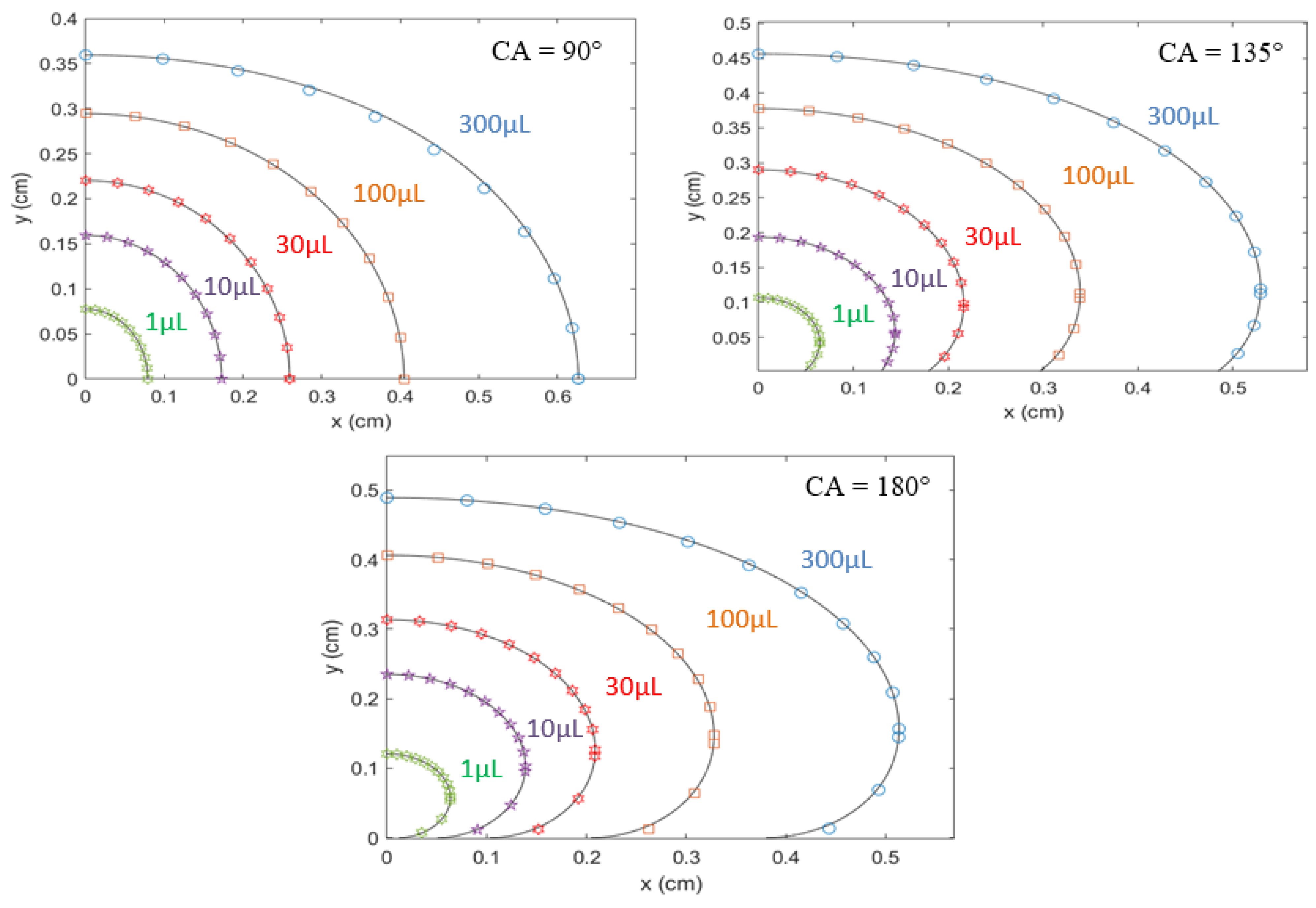
The profiles of the ellipses almost exactly match the profile generated using the Young–Laplace equation, Figure 2. Contact angles of elliptic droplets were generated using defined constraints from the bottom ellipse and tangent line, Equations (10) and (11). The correction factor for the bottom ellipse C₃ = 0.963238 was determined similarly to C₁ and C₂. Without the correction factor C₃, the errors for volume and surface area calculation were significant as they reached up to 10% (Table S3). We compared parameters derived from droplet profiles such as surface areas and droplet volumes to demonstrate the accuracy of the elliptic method.

Table 2. Droplet parameters at different volumes and various contact angles: (i) Young–Laplace theoretical droplet; (ii) generated droplet using the elliptic model.

Pre-Defined Volume (µL)	Contact Angle (°)			Volume (µL)			Surface Area (cm2)
	(i)	(ii)	Error (%)	(i)	(ii)	Error (%)	(i)	(ii)	Error (%)
1	90	90	0	1.0	1.0	0	0.039	0.039	0
	135	134.13	0.65	1.0	1.0	0	0.044	0.043	0.23
	180	174.75	3	1.0	1.0	0	0.050	0.049	0.41
10	90	90	0	9.9	10.0	1.00	0.178	0.178	0.28
	135	137.12	1.55	10.4	10.4	0	0.199	0.199	0.10
	180	179.21	0.44	10.0	10.0	0	0.218	0.219	0.23
30	90	90	0	30.8	30.8	0	0.379	0.379	0.03
	135	138.76	2.71	31.6	31.7	0.32	0.410	0.410	0.19
	180	180.00	0	30.9	31.1	0.64	0.452	0.454	0.57
100	90	90	0	100.7	101.0	0.30	0.846	0.848	0.19
	135	141.35	4.49	101.2	101.5	0.30	0.871	0.871	0.01
	180	180.00	0.00	100.4	101.3	0.89	0.963	0.972	0.88
300	90	90	0	300.7	294.4	2.14	1.821	1.801	1.10
	135	139.82	3.45	298.9	297.0	0.64	1.784	1.772	0.67
	180	180.00	0	300.8	300.0	0.27	1.959	1.964	0.28

shows that the volume and surface area are in good agreement with the numerical method. Errors tend to increase with the volume and contact angle because the droplet shape starts to deviate from an ellipsoid in these extreme regions.

The Bond numbers of the droplets generated using the Young–Laplace numerical method and the elliptic method were also compared (

Table 3. Comparison of Bond number between (i) Young–Laplace theoretical droplet and (ii) generated droplet using the elliptic model.

Pre-Defined Volume (µL)	Bond Number
	(i)	(ii)	Error (%)
1	0.0536	0.0534	0.374
10	0.2461	0.2462	0.041
30	0.5195	0.5201	0.115
100	1.1423	1.1444	0.184
300	2.3654	2.3505	0.64

). The Bond number of each droplet volume was taken as the average value of all of the contact angles investigated. Table 3 shows that the Bond number values are in excellent agreement with each other. Hence, we can conclude that the elliptic method is applicable for a large range of Bond numbers from 0.055 to 2.379.

4.3. Compatibility of Elliptic Model with Actual Sessile Droplet

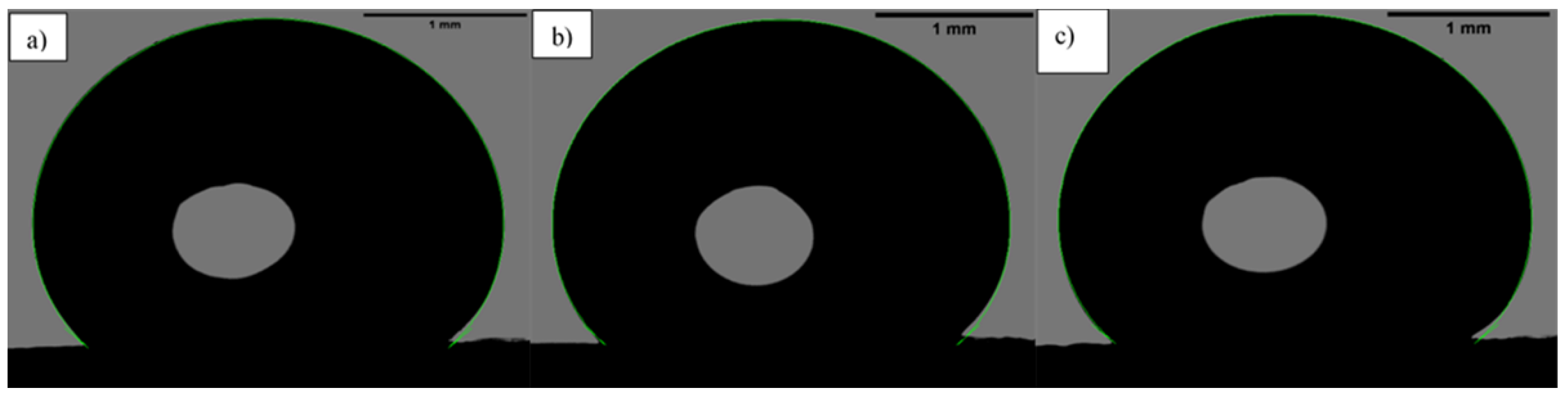
Images of sessile droplets were captured and analysed following the method described in Section 3 to investigate the applicability of the elliptic model method to actual liquid droplets. The volume of droplets was fixed at 10 μL for comparison. Figure 3 shows the fitted droplets with the green curves that are generated by the LBADSA method. Meanwhile, the critical parameters produced using LBADSA and the elliptic model are compared in

Table 4. Comparison of droplet parameters between two methods: (i) LBADSA; (ii) axisymmetrical elliptic model.

Run	Volume (µL)			Surface Area (cm2)			Contact Angle (°)			Surface Tension (mN/m)
	(i)	(ii)	Error (%)	(i)	(ii)	Error (%)	(i)	(ii)	Error (%)	(i)	(ii)	Error (%)
1	10.7	10.7	0	0.203	0.204	0.49	137	138.46	1.07	81.75	78.7	3.87
2	10.5	10.6	0.95	0.201	0.202	0.5	137.72	139.46	1.26	72.67	69.6	4.41
3	10.8	10.8	0	0.205	0.206	0.49	138.91	140.84	1.39	72.67	70	3.81

. The results show that for all of the elliptic droplets, their parameters are extremely close to those of the LBADSA-based counterparts, which demonstrates that the asymmetric elliptic model has the ability to model real sessile droplets with good accuracy.

5. Conclusions

In this study, we developed a simple and convenient method to model a sessile droplet based on elliptic analytical representation. From the comparison with a reference droplet based on Young–Laplace differential equations and actual droplet profiles, we demonstrated that the elliptic model can be used for practical applications such as determining the surface tension and contact angle of an unidentified sessile droplet. The elliptic model also accurately constructed droplet profiles at different droplet volumes (1–300 µL), within the effective range of the contact angle from 90° to 180°. The high precision and ease of operation enable this elliptic model to be used as an alternative for studying sessile droplets with large contact angles.

References

- Lubarda, V.A.; Talke, K.A. Analysis of the Equilibrium Droplet Shape Based on an Ellipsoidal Droplet Model. Langmuir 2011, 27, 10705–10713. [Google Scholar] [CrossRef]
- Dixit, S.S.; Pincus, A.; Guo, B.; Faris, G.W. Droplet Shape Analysis and Permeability Studies in Droplet Lipid Bilayers. Langmuir 2012, 28, 7442–7451. [Google Scholar] [CrossRef] [Green Version]
- Zhou, W.; Loney, D.; Degertekin, F.L.; Rosen, D.W.; Fedorov, A.G. What controls dynamics of droplet shape evolution upon impingement on a solid surface? AIChE J. 2013, 59, 3071–3082. [Google Scholar] [CrossRef]
- Saad, S.M.I.; Policova, Z.; Neumann, A.W. Design and accuracy of pendant drop methods for surface tension measurement. Colloids Surf. A Physicochem. Eng. Asp. 2011, 384, 442–452. [Google Scholar] [CrossRef]
- Berry, J.D.; Neeson, M.J.; Dagastine, R.R.; Chan, D.Y.C.; Tabor, R.F. Measurement of surface and interfacial tension using pendant drop tensiometry. J. Colloid Interface Sci. 2015, 454, 226–237. [Google Scholar] [CrossRef] [PubMed]
- Brandon, S.; Marmur, A. Simulation of Contact Angle Hysteresis on Chemically Heterogeneous Surfaces. J. Colloid Interface Sci. 1996, 183, 351–355. [Google Scholar] [CrossRef] [PubMed]
- He, B.; Yang, S.; Qin, Z.; Wen, B.; Zhang, C. The roles of wettability and surface tension in droplet formation during inkjet printing. Sci. Rep. 2017, 7, 11841. [Google Scholar] [CrossRef] [PubMed] [Green Version]
- Jain, V.; Raj, T.P.; Deshmukh, R.; Patrikar, R. Design, fabrication and characterization of low cost printed circuit board based EWOD device for digital microfluidics applications. Microsyst. Technol. 2017, 23, 389–397. [Google Scholar] [CrossRef]
- Nguyen, C.T.; Kim, B. Stress and surface tension analyses of water on graphene-coated copper surfaces. Int. J. Precis. Eng. Manuf. 2016, 17, 503–510. [Google Scholar] [CrossRef]
- Gates, C.H.; Perfect, E.; Lokitz, B.S.; Brabazon, J.W.; McKay, L.D.; Tyner, J.S. Transient analysis of advancing contact angle measurements on polished rock surfaces. Adv. Water Resour. 2018, 119, 142–149. [Google Scholar] [CrossRef]
- Hünnekens, B.; Peters, F.; Avramidis, G.; Krause, A.; Militz, H.; Viöl, W. Plasma treatment of wood–polymer composites: A comparison of three different discharge types and their effect on surface properties. J. Appl. Polym. Sci. 2016, 133. [Google Scholar] [CrossRef]
- Bashforth, F.; Adams, J. An Attempt to Test the Theory of Capillary Action; Cambridge University: Cambridge, UK, 1892. [Google Scholar]
- Shanahan, M.E.R. An approximate theory describing the profile of a sessile drop. J. Chem. Soc. Faraday Trans. 1 Phys. Chem. Condens. Phases 1982, 78, 2701–2710. [Google Scholar] [CrossRef]
- Joshi, Y.P. Shape of a liquid surface in contact with a solid. Eur. J. Phys. 1990, 11, 125–129. [Google Scholar] [CrossRef]
- Yildiz, B.; Bashiry, V. Shape analysis of a sessile drop on a flat solid surface. J. Adhes. 2019, 95, 929–942. [Google Scholar] [CrossRef]
- Hartland, S.; Hartley, R.W. Axisymmetric Fluid-Liquid Interfaces: Tables Giving the Shape of Sessile and Pendant Drops and External Menisci, with Examples of Their Use; Elsevier Science Limited: Amsterdam, The Netherlands, 1976. [Google Scholar]
- Jennings, J.W.; Pallas, N.R. An efficient method for the determination of interfacial tensions from drop profiles. Langmuir 1988, 4, 959–967. [Google Scholar] [CrossRef]
- Yu, K.; Yang, J.; Zuo, Y.Y. Automated Droplet Manipulation Using Closed-Loop Axisymmetric Drop Shape Analysis. Langmuir 2016, 32, 4820–4826. [Google Scholar] [CrossRef] [Green Version]
- Skinner, F.K.; Rotenberg, Y.; Neumann, A.W. Contact angle measurements from the contact diameter of sessile drops by means of a modified axisymmetric drop shape analysis. J. Colloid Interface Sci. 1989, 130, 25–34. [Google Scholar] [CrossRef]
- Río, O.I.D.; Neumann, A.W. Axisymmetric Drop Shape Analysis: Computational Methods for the Measurement of Interfacial Properties from the Shape and Dimensions of Pendant and Sessile Drops. J. Colloid Interface Sci. 1997, 196, 136–147. [Google Scholar] [CrossRef] [PubMed] [Green Version]
- Aussillous, P.; Quéré, D. Liquid marbles. Nature 2001, 411, 924–927. [Google Scholar] [CrossRef] [PubMed]
- Aussillous, P.; Quéré, D. Properties of liquid marbles. Proc. R. Soc. A Math. Phys. Eng. Sci. 2006, 462, 973–999. [Google Scholar] [CrossRef]
- Singha, P.; Ooi, C.H.; Nguyen, N.-K.; Sreejith, K.R.; Jin, J.; Nguyen, N.-T. Capillarity: Revisiting the fundamentals of liquid marbles. Microfluid. Nanofluidics 2020, 24, 81. [Google Scholar] [CrossRef]
- Singha, P.; Nguyen, N.-K.; Sreejith, K.R.; An, H.; Nguyen, N.-T.; Ooi, C.H. Effect of Core Liquid Surface Tension on the Liquid Marble Shell. Adv. Mater. Interfaces 2021, 8, 2001591. [Google Scholar] [CrossRef]
- Ooi, C.H.; Vadivelu, R.; Jin, J.; Sreejith, K.R.; Singha, P.; Nguyen, N.-K.; Nguyen, N.-T. Liquid marble-based digital microfluidics—Fundamentals and applications. Lab Chip 2021, 21, 1199–1216. [Google Scholar] [CrossRef]
- Ooi, C.H.; Singha, P.; Nguyen, N.-K.; An, H.; Nguyen, V.T.; Nguyen, A.V.; Nguyen, N.-T. Measuring the effective surface tension of a floating liquid marble using X-ray imaging. Soft Matter 2021, 17, 4069–4076. [Google Scholar] [CrossRef]
- Singha, P.; Nguyen, N.-K.; Zhang, J.; Nguyen, N.-T.; Ooi, C.H. Oscillating sessile liquid marble—A tool to assess effective surface tension. Colloids Surf. A Physicochem. Eng. Asp. 2021, 627, 127176. [Google Scholar] [CrossRef]
- Ooi, C.H.; Vadivelu, R.K.; St John, J.; Dao, D.V.; Nguyen, N.-T. Deformation of a floating liquid marble. Soft Matter 2015, 11, 4576–4583. [Google Scholar] [CrossRef] [PubMed] [Green Version]
- Cengiz, U.; Erbil, H.Y. The lifetime of floating liquid marbles: The influence of particle size and effective surface tension. Soft Matter 2013, 9, 8980–8991. [Google Scholar] [CrossRef]
- Jin, J.; Nguyen, N.-T. Manipulation schemes and applications of liquid marbles for micro total analysis systems. Microelectron. Eng. 2018, 197, 87–95. [Google Scholar] [CrossRef]
- Nguyen, N.-K.; Singha, P.; Zhang, J.; Phan, H.-P.; Nguyen, N.-T.; Ooi, C.H. Digital Imaging-based Colourimetry for Enzymatic Processes in Transparent Liquid Marbles. ChemPhysChem 2021, 22, 99–105. [Google Scholar] [CrossRef]
- Nguyen, N.-K.; Ooi, C.H.; Singha, P.; Jin, J.; Sreejith, K.R.; Phan, H.-P.; Nguyen, N.-T. Liquid Marbles as Miniature Reactors for Chemical and Biological Applications. Processes 2020, 8, 793. [Google Scholar] [CrossRef]
- Nguyen, N.-K.; Singha, P.; An, H.; Phan, H.-P.; Nguyen, N.-T.; Ooi, C.H. Electrostatically excited liquid marble as a micromixer. React. Chem. Eng. 2021, 6, 1386–1394. [Google Scholar] [CrossRef]
- Ooi, C.H.; Nguyen, N.-T. Manipulation of liquid marbles. Microfluid. Nanofluidics 2015, 19, 483–495. [Google Scholar] [CrossRef]
- Arbatan, T.; Li, L.; Tian, J.; Shen, W. Liquid Marbles as Micro-bioreactors for Rapid Blood Typing. Adv. Healthc. Mater. 2012, 1, 80–83. [Google Scholar] [CrossRef] [PubMed]
- Zang, D.; Li, J.; Chen, Z.; Zhai, Z.; Geng, X.; Binks, B.P. Switchable Opening and Closing of a Liquid Marble via Ultrasonic Levitation. Langmuir 2015, 31, 11502–11507. [Google Scholar] [CrossRef] [PubMed]
- Sato, E.; Yuri, M.; Fujii, S.; Nishiyama, T.; Nakamura, Y.; Horibe, H. Liquid marbles as a micro-reactor for efficient radical alternating copolymerization of diene monomer and oxygen. Chem. Commun. 2015, 51, 17241–17244. [Google Scholar] [CrossRef] [PubMed]
- Han, X.; Koh, C.S.L.; Lee, H.K.; Chew, W.S.; Ling, X.Y. Microchemical Plant in a Liquid Droplet: Plasmonic Liquid Marble for Sequential Reactions and Attomole Detection of Toxin at Microliter Scale. ACS Appl. Mater. Interfaces 2017, 9, 39635–39640. [Google Scholar] [CrossRef]
- Tian, J.; Fu, N.; Chen, X.D.; Shen, W. Respirable liquid marble for the cultivation of microorganisms. Colloids Surf. B Biointerfaces 2013, 106, 187–190. [Google Scholar] [CrossRef] [PubMed]
- Sheng, Y.; Sun, G.; Wu, J.; Ma, G.; Ngai, T. Silica-Based Liquid Marbles as Microreactors for the Silver Mirror Reaction. Angew. Chem. Int. Ed. 2015, 54, 7012–7017. [Google Scholar] [CrossRef] [PubMed]
- Gu, H.; Ye, B.; Ding, H.; Liu, C.; Zhao, Y.; Gu, Z. Non-iridescent structural color pigments from liquid marbles. J. Mater. Chem. C 2015, 3, 6607–6612. [Google Scholar] [CrossRef]
- McHale, G.; Elliott, S.J.; Newton, M.I.; Herbertson, D.L.; Esmer, K. Levitation-Free Vibrated Droplets: Resonant Oscillations of Liquid Marbles. Langmuir 2009, 25, 529–533. [Google Scholar] [CrossRef] [PubMed]
- Farid, M. A new approach to modelling of single droplet drying. Chem. Eng. Sci. 2003, 58, 2985–2993. [Google Scholar] [CrossRef]
- Hu, H.; Larson, R.G. Evaporation of a Sessile Droplet on a Substrate. J. Phys. Chem. B 2002, 106, 1334–1344. [Google Scholar] [CrossRef]
- Marinaro, G.; Riekel, C.; Gentile, F. Size-Exclusion Particle Separation Driven by Micro-Flows in a Quasi-Spherical Droplet: Modelling and Experimental Results. Micromachines 2021, 12, 185. [Google Scholar] [CrossRef] [PubMed]
- Marchese, A.J.; Dryer, F.L.; Nayagam, V. Numerical modeling of isolated n-alkane droplet flames: Initial comparisons with ground and space-based microgravity experiments. Combust. Flame 1999, 116, 432–459. [Google Scholar] [CrossRef]
Figure 1.
Schematic of the coordinate system for the elliptic model. O is the coordinate of the origin, whereas (i, j) is the coordinate of the three-phase contact point.
Figure 2.
Comparison between droplet profiles with the Young–Laplace theoretical model (continuous lines) and elliptic model (scattered data points) at different nominal contact angles.
Figure 3.
(a–c) Images of 10 μL droplets with constructed fitting curves using ImageJ’s plugin LBADSA. Scale bar is 1 mm.