Between three to four batch cultures per strain were carried out (
Table 2). Two batches per strain were used to perform parameter calibration, and between one and two batches were used to validate the models. The experimental datasets for each strain are presented in
Figure 1,
Figure 2 and
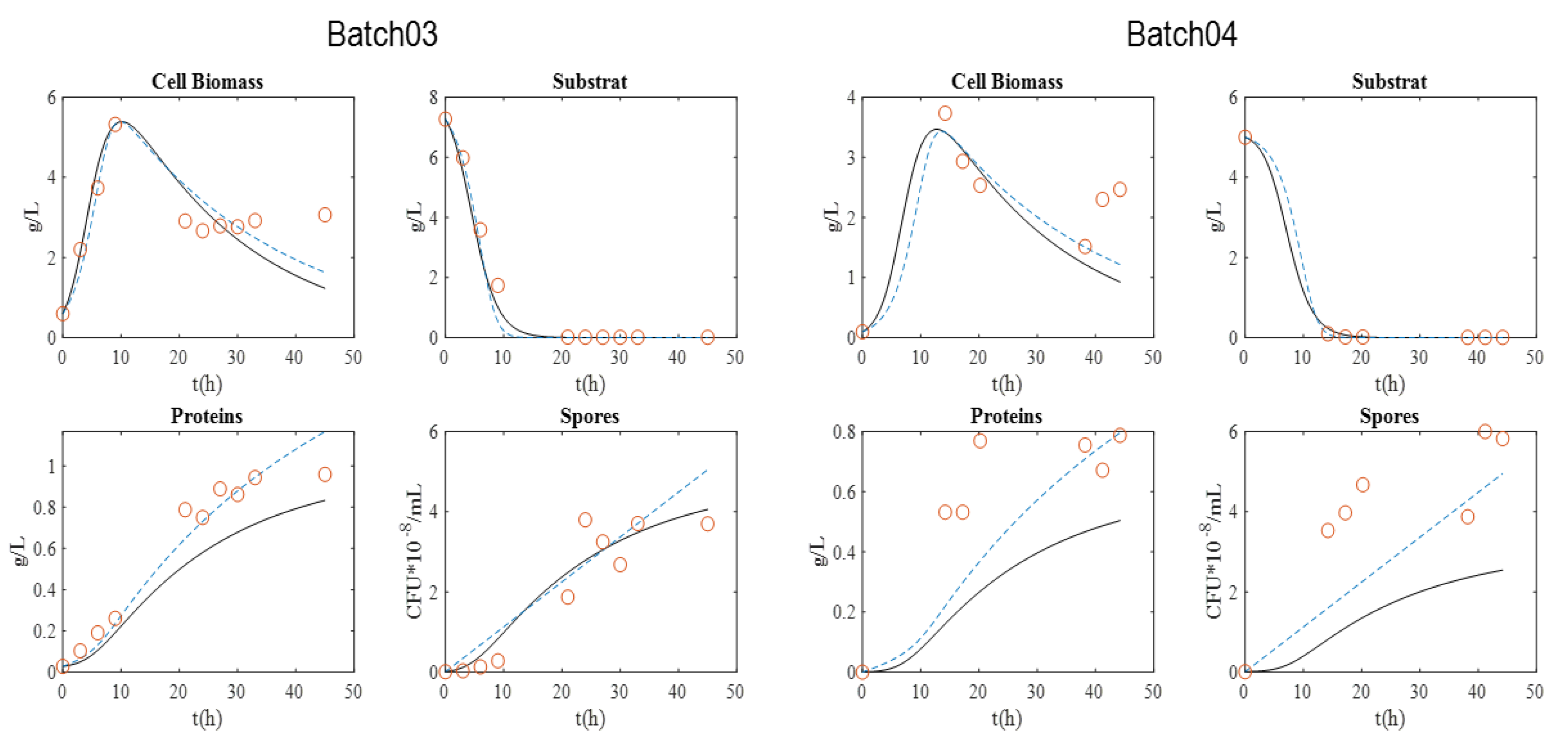
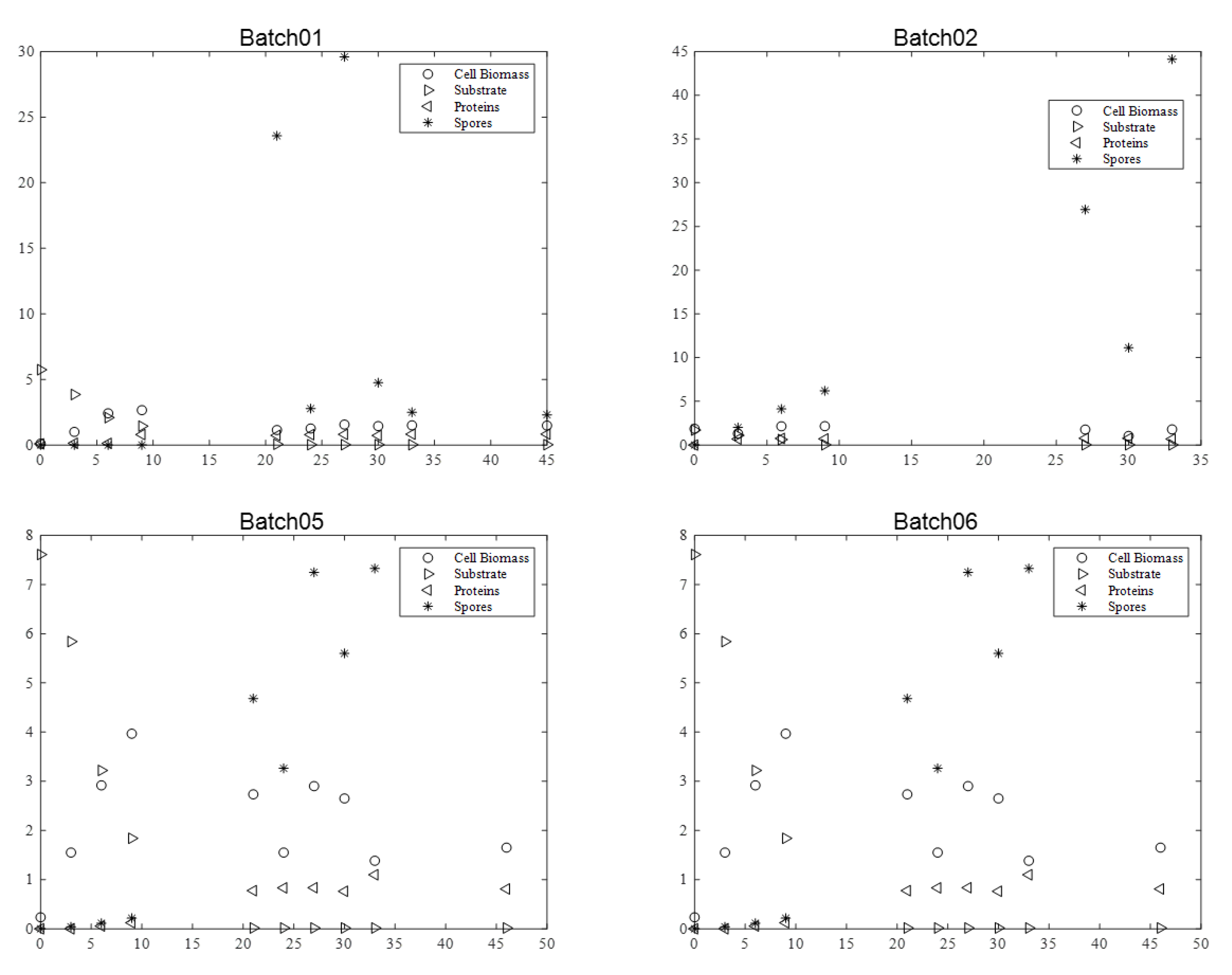
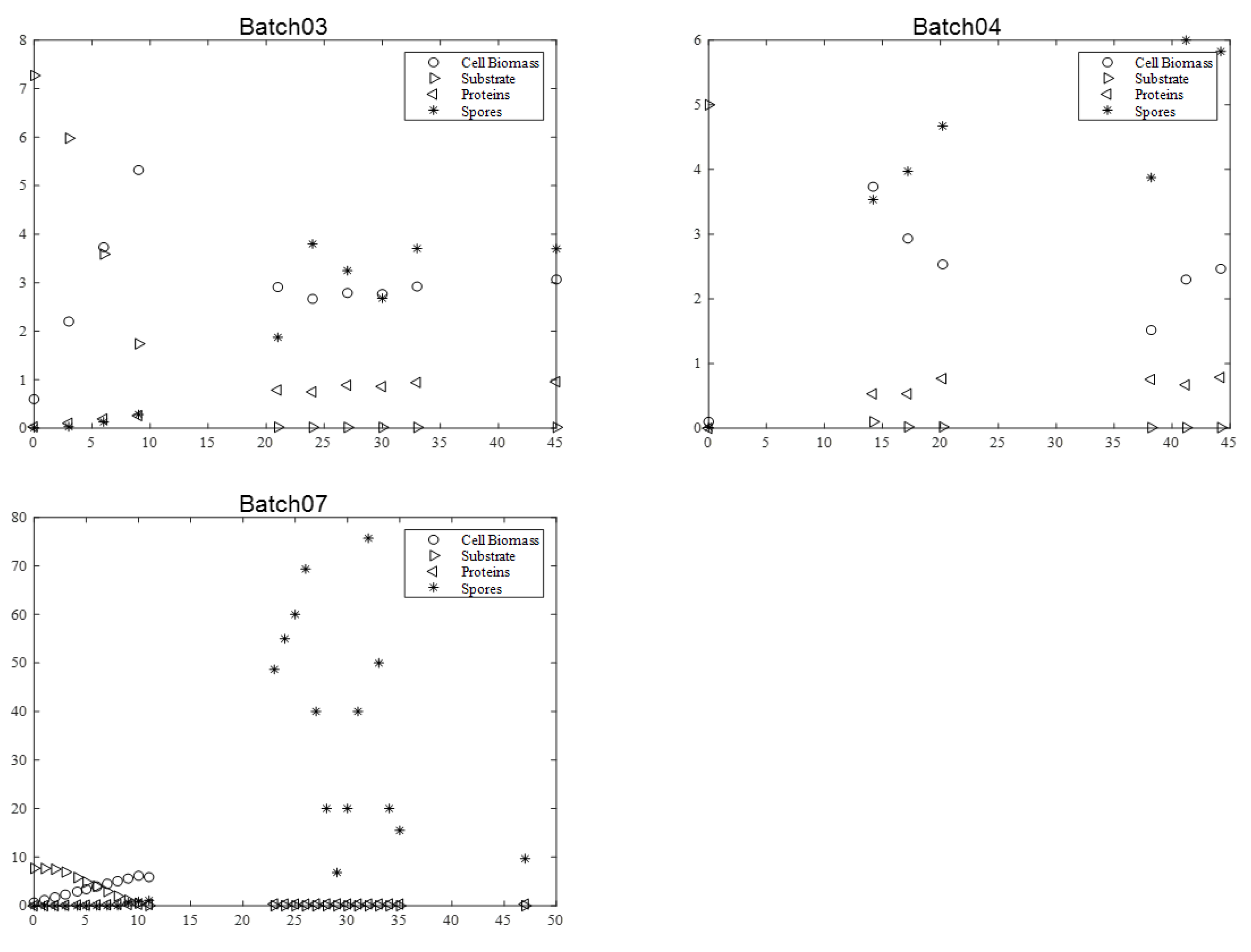
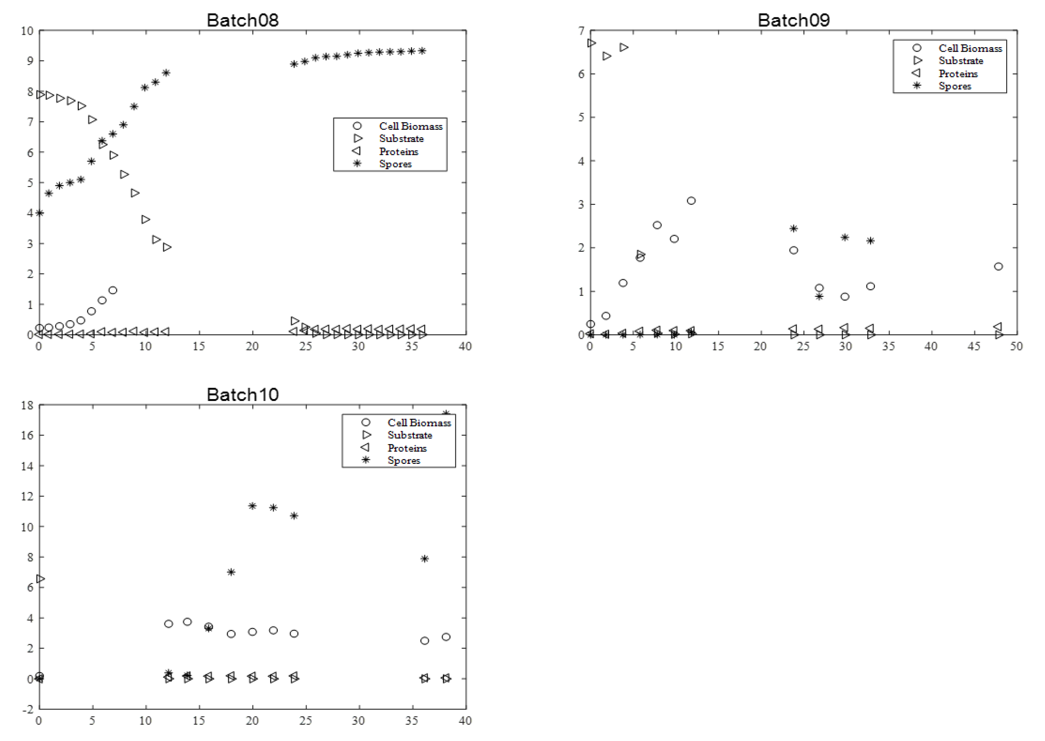
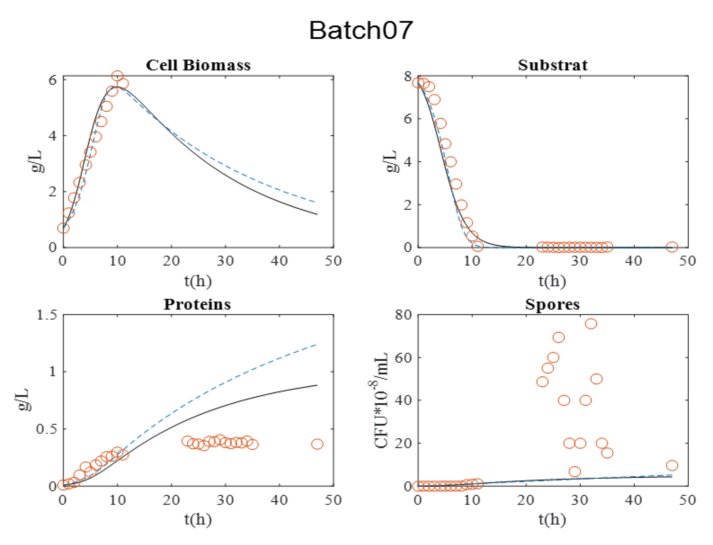
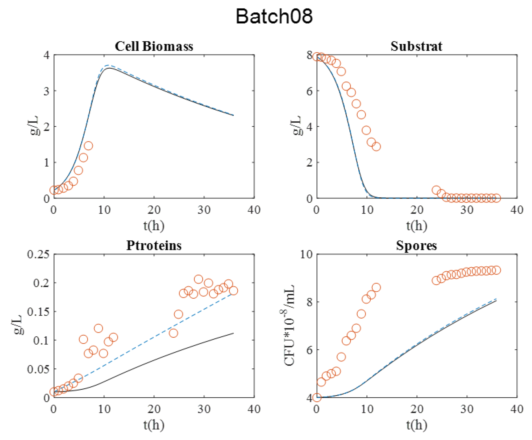
Figure 3. It is relevant to indicate that in batch 07, dry matter measurement was estimated by OD600nm for exponential growth phase.
During all cultures, several milestones should be identified: (i) the maximum cell biomass production, (ii) substrate depletion, (iii) full sporulation informing about proteins production, and (iv) its release in supernatant due to full cell lysis.
2.5.1. Btk. BLB1 Strain
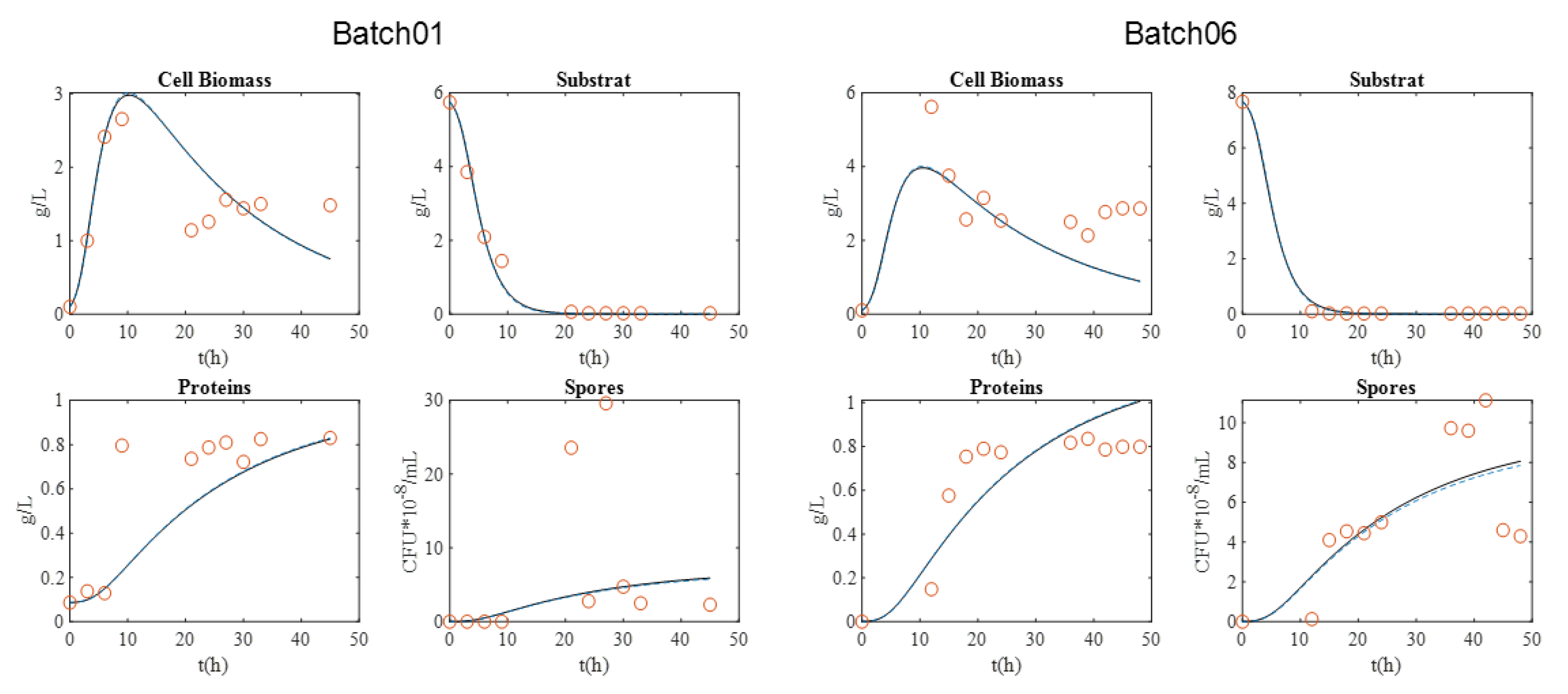
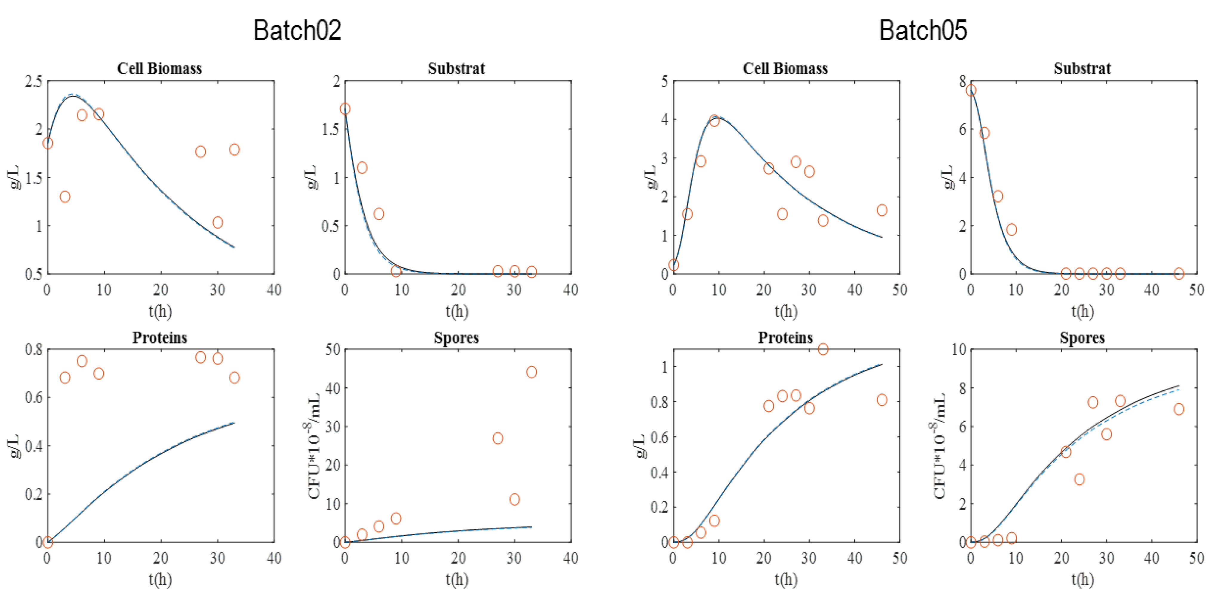
For the BLB1 strain, data were taken from four batches (01, 02, 05, and 06).
Figure 1 presents the graphical experimental data. Batch 11 was used to validate the model.
The maximum biomass concentration was reached after approximately 10 h culture for the four batches, and then began to decrease. As expected, this time approximately coincided with the substrate depletion, corresponding to a glucose concentration close to 0 g·L−1. In addition, the concentration of spores began to increase at this moment, since the limitation of the substrate induced their formation. After 20 h, sporulation reached a plateau value. Cell lysis was fully achieved after 30 h, as indicated by protein release into supernatant. Finally, protein content reached around 0.8–1 g·L−1 with BLB1 stain.
2.5.4. Model Assumptions
The main features of dynamic models include the key parameters describing bioperformances (vegetative cell, spores, substrate, proteins) and associated kinetics, considering successive phases (oxidative growth, limitation, sporulation, and protein release), during bioproduction. The mass balance equations on each compound are shown in Equations (1), (2), (4)–(7). Equation (1) represents the evolution of biomass concentration with respect to time, while the relationship between bacterial growth and substrate consumption is shown in Equations (1) and (2).
where X is the biomass concentration (g·L
−1),
is the concentration of substrate (g·L
−1), Y1 is the yield coefficient between the biomass and the substrate (gBiomass/gGlucose), and
is the death rate (h
−1).
The cell growth process is represented by the Contois expression, as follows:
where
is the specific growth rate (h
−1) and
is the maximum specific growth rate (h
−1), a constant defined for a substrate concentration; X1 is the concentration of biomass (g·L
−1); S1 is the concentration of glucose (g·L
−1); and
is a saturation constant.
Equations (4)–(7) show the mass balance for proteins and spores. In the first model, proteins and spores are correlated with biomass (Model 1). In the second model, α and β parameters were used to unassociated proteins and spores from biomass production (Model 2). The corresponding models are shown in Equations (4) and (5) (Model 1) and Equations (6) and (7) (Model 2).
Model 2
where
is the protein concentration (g·L
−1),
is the spores concentration (CFU·10
−8/mL),
(gPro·gGlucose
−1 ·h
−1) and
(CFU·10
−5·g Glucose
−1·h
−1) are yield coefficients, and
(g·L
−1·h
−1) is a constant.
The set of equations were simulated using MATLAB®(R2019a).
Three statistical criteria were used to analyze the fit of the models using experimental datasets. These parameters were the coefficient of determination (R2), the root mean square errors (RSME), and the correction of Akaike information criterion (AICc). The expressions of these parameters are presented in Equations (8)–(11), respectively.
SSR is sum of squared regression, and SST is sum of squared total.
where n represents the number of data, p the number of parameters, W the weighting matrix, and
and
are the data and estimated data, respectively [
13].
The main parameter used to determine the model that best fits the data is the AICc parameter [
13]. The AIC criterion is one of the most popular for the comparison of models because it considers the number of parameters, the number of data, and the residuals, making it a parameter that balances the complexity of the model and the fit of the data [
14]. Additionally, the parameter correction (AICc) gives accurate results for a larger number of datasets. Thus, the model with the lowest value for AICc is selected to represent the experimental data more adequately.
Parameter calibration was carried out in MATLAB using a particle swarm optimization (PSO) algorithm. This method, as its name implies, is inspired by the behavior of swarms of insects in nature. Thus, for a set of variables to be optimized, the method begins by placing random particles in the search space, but then a series of rules are established considering each parameter and the set of parameters (“swarm”) globally. Thus, the variables are optimized quite well, and few computational resources are spent, becoming a fast method in convergence, and simple in application [
15].


 ,
, 


