Research on Measurement and Application of China’s Regional Logistics Development Level under Low Carbon Environment

Abstract

To solve the problem of fuzziness and randomness in regional logistics decarbonization evaluation and accurately assess regional logistics decarbonization development, an evaluation model of regional logistics decarbonization development is established. First, the evaluation index of regional logistics decarbonization development is constructed from three dimensions: low-carbon logistics environment support, low-carbon logistics strength and low-carbon logistics potential. Second, the evaluation indexes are used as cloud model variables, and the cloud numerical characteristic values and cloud affiliation degrees are determined according to the cloud model theory. The entropy weight method is used to determine the index weights, and the comprehensive determination degree of the research object affiliated to the logistics decarbonization level is calculated comprehensively. Finally, Beijing-Tianjin-Hebei region is used as an example for empirical evidence, analyzing the development logistics decarbonization and its and temporal variability in Beijing, Tianjin and Hebei provinces and cities. The results of the study show that the development logistics decarbonization in Beijing, Tianjin and Hebei Province has been improved to different degrees during 2013–2019, but the development is uneven. Developing to 2019, the three provinces and cities of Beijing, Tianjin and Hebei still have significant differences in terms of economic environment, logistics industry scale, logistics industry inputs and outputs, and technical support.

1. Introduction

China has entered a new stage of high-quality development; the people’s demand for ecological environment is getting higher and higher, and the importance and urgency of promoting green development has become more and more prominent. In 2020, General Secretary Xi Jinping solemnly declared to the world at the United Nations General Assembly that China’ s carbon dioxide emissions will peak by 2030 and strive to achieve carbon neutrality by 2060. As a high-end service industry, logistics has the characteristics of high energy consumption and high emission. The development path of logistics must follow low-carbon development, focusing on green logistics, low-carbon logistics and intelligent informatization. With the rise of the low-carbon revolution and the official advocation of green environment at the Copenhagen environment conference, low-carbon logistics has become the focus of academic research at home and abroad. The research of low-carbon logistics focuses on four aspects: carbon emission accounting, carbon emission driver identification, low-carbon logistics capability measurement and low-carbon logistics development strategy. In carbon emission accounting of logistics process, Butner K, Dada A, Piecyk M I adopt the method of carbon emission measurement based on whole life cycle and design the analytical of carbon emission measurement including structural factors and commercial factors [1,2,3]. Wang LP and Liu Y calculated the carbon emission from energy data of Chinese provinces from 1997–2004 and 2007–2013 [4,5]. Concerning identifying drivers of carbon emissions in the logistics industry, Timilsina and others studied on the growth of carbon emissions in the transport in selected Asian countries from 1980 to 2005 [6]. Lei Yang takes Shenzhen port as an example and measures the carbon emission in the port comprehensive logistics system [7]. Yang YW, Li FG, Men D et.al explore the driving causes of carbon emission growth by using LMDI model decomposition analysis [8,9,10]. In the low carbon logistics capability, Jessica Wehner takes an interactive approach to capacity utilization to contribute to sustainable freight transport and logistics [11]. The Chinese scholars mainly focus on the fuzzy comprehensive evaluation method, entropy weight TOPSIS model, DEA evaluation model, and Malmquist model static measurement methods to evaluate [12,13,14,15]. In the development strategy of low-carbon logistics, relevant scholars analyze the current situation and problems of low-carbon logistics development from different perspectives and put forward suggestions to promote the development of low-carbon logistics [16,17,18,19,20]. At present, scholars have conducted fewer studies related to the low-carbon development of regional logistics. Ma YY used data envelopment analysis to study the total factor productivity of China’s logistics industry under low-carbon constraints [21]. Xie F and Gao FF analyzed the low carbonization of China’s logistics industry and related industries by constructing an index system for the coordinated development of logistics industry and low carbon economy and using a coordinated development model [22,23]. Yu Q analyzed the logistics efficiency and its influencing factors in 30 provinces and cities, as well as the eastern, central and western regions of China based on the DEA-Tobit two-stage method [24]. Song Lina used a combined model of principal component analysis and data envelopment analysis to evaluate the regional low-carbon logistics performance of provinces along the Silk Road Economic Belt in China [25]. Wang X, taking Anhui Province as an example, explored the mechanism of the low-carbon development of regional logistics using the theoretical analysis framework of “development dynamics-measurement criteria-acting subject” [26].

To solve the fuzzy and stochastic problems in the process of low carbonization evaluation of regional logistics, the fuzzy and stochastic properties were converted into a definite value by the cloud generator, which broke the limitation of qualitative and quantitative research and made the evaluation more hierarchical [27].

2. Theoretical Basis

2.1. Entropy Weighting Method

Entropy is a measure of the disorder degree of a system. According to defined entropy, we can use the size of entropy to judge the discreteness degree of an index. The smaller the entropy value is, the greater the influence of the index on the comprehensive evaluation (i.e., the weight). Therefore, information entropy is a tool that can be used to objectively empower multiple signs to provide the basis for a comprehensive evaluation:

• Standardized processing of data: assume that m evaluation objects, n evaluation signals, get the original evaluation, $X={\left(X_{ij}\right)}_{m\times n}$, make

  $$U_{ij}=\left\{\begin{array}{c}\frac{X_{ij}-\underset{i}{min}{X}_{ij}}{\underset{i}{max}{X}_{ij}-\underset{i}{min}{X}_{ij}},Negative indicators\\ \frac{\underset{i}{max}{X}_{ij}-X_{ij}}{\underset{i}{max}{X}_{ij}-\underset{i}{min}{X}_{ij}},Positive Indicators\end{array}\right.$$

  (1)

  where $X_{ij}$ denotes the $j$ indicator of the $i$ evaluator in a given locality, $U_{ij}$ it is the standardized data.
• Calculation of weights for each indicator:

  $$P_{ij}=\frac{U_{ij}}{{\displaystyle \sum _{i=1}^m{U}_{ij}}}$$

  (2)
• Calculation of entropy for each indicator:

  $$e_j=-\frac{1}{\ln m}{\displaystyle \sum _{i=1}^m{P}_{ij}\ln P_{ij}}$$

  (3)
• Determination of weights for each indicator:

  $$w_j=\frac{1-e_j}{n-{\displaystyle \sum _{j=1}^n{e}_j}}$$

  (4)

2.2. Cloud Models

2.2.1. The Cloud Models

Li DY and others are the basis of cloud computing, reasoning, and control, and it is a model for the transformation of uncertainty between qualitative concepts and quantitative descriptions [27,28,29]. It is widely used in risk assessment, data mining, and performance evaluation and so on [30,31,32,33]. Let $O$ be a quantitative set represented by a numerical value. $I$ is a qualitative concept in $O$ space. If the quantitative value $x\in O$ and $x$ is a stochastic implementation in the qualitative concept $I$, the determinacy of $x$ to $I$: $\mu (x)\in \left[0,1\right]$, It is a stochastic number with a tendency to stability:

$$\mu :O\to \left[0,1\right],\forall x\in O,x\to \mu (x)$$

Then the distribution of $x$ in the set is called the cloud model, with each $x$ being a cloud drop.

2.2.2. Numerical Characteristics of Clouds

Cloud models represent the primitive-language values in natural language, and the three numeric features of cloud models—$Ex$ (expectation), $En$ (entropy), and $He$ (supers entropy)—represent the numerical characteristics of language values, thus achieving the goal of integrating the fuzziness and randomness of objects studied. Among them, $Ex$ is the expectation of cloud droplet distribution in the domain. It is the central value of cloud droplet in a given set space distribution. $En$ indicates the uncertainty measure of qualitative concept, which reflects the dispersion degree of cloud droplet, which is determined by the ambiguity and randomness of qualitative concept. $He$ is a measure of the fuzziness of entropy, the size of which indirectly reflects the thickness of cloud droplets and the fuzziness and randomness of entropy [34,35,36].

2.2.3. Cloud Generator

The mutual transformation between qualitative concept and quantitative data in cloud model needs to be realized by cloud generator. Typically, a cloud generator includes a forward cloud generator, a reverse cloud generator and a conditional cloud generator.

Forward Cloud Generator: A mapping from a qualitative concept to a quantitative value, a process by which cloud droplets are generated from the numerical eigenvalues of a cloud model, as shown in Figure 1.

In Figure 1, $CG$ means the forward cloud generator, $x_i$ is the cloud droplet, and ${\mu }_i$ is its affiliation degree.

Reverse Cloud Generator: Mapping from quantitative values to directed ideas, that is, converting exact data into the suitable qualitative language $(Ex,En,He)$, as shown in Figure 2.

In Figure 2, $C{G}^{-1}$ notes a reverse cloud generator, $x_i$ is the cloud droplet, and ${\mu }_i$ is its affiliation degree.

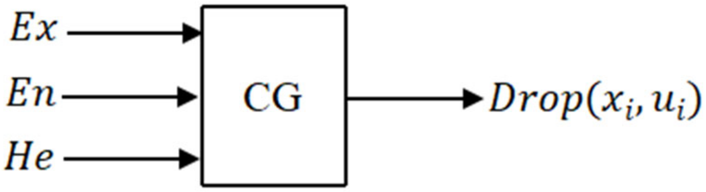
$X$ Conditional Cloud Generator: In the numerical domain space of a given set, the three digital eigenvalues of the known cloud, $Ex$,$En$,$He$, and contain a specified condition $x=x_0$, this is called Conditional Cloud Generator. As shown in Figure 3.

2.3. Carbon Emission Measurement

At present, there is no uniform standard for carbon emission measurement in the world. This paper adopts the more extensive estimation method of IPCC, also known as the IPCC inventory coefficient method. This method is based on the final energy consumption, and considering the waste gas emitted during the logistics process includes not only carbon dioxide, but also carbon monoxide, hydrocarbons, etc. In this paper, the carbon emission of the logistics industry is estimated by energy consumption. This is done by multiplying the various energy consumption of the logistics industry by their respective standard coal coefficient and then by their respective carbon emission factors to arrive at the total carbon emissions for a given year in the region:

$$C={\displaystyle \sum }_i{C}_i={\displaystyle \sum }_i{\delta }_i{\theta }_i{E}_i$$

(5)

Of which: $C_i$ means carbon emissions from type $i$ energy sources, $E_i$ denotes consumption of type $i$ energy sources, ${\theta }_i$ marks coefficient of fractional standard coal for type $i$ energy sources, ${\delta }_i$ stands for carbon emission factors for type $i$ energy sources, and ${\theta }_i{E}_i$ denotes amount of fractional standard coal for type $i$ energy sources.

3. Regional Logistics Decarbonization Development Evaluation Model Construction

3.1. Evaluation Index System for Low-Carbon Development of Regional Logistics

Low-carbonization of regional logistics means building a regional logistics system which is based on low-carbon economy and green logistics and supports the concept of “sustainable development” and“carbon emissions”. It meets the regional economic and political development and has a supporting system of logistics information and organization and operation, while possessing the characteristics of green, balanced and efficient. Related scholars have different focuses and starting points for the research on the level of regional logistics decarbonization, such as Lai, Ma Shihua et al. from the logistics system [37,38], and Daugherty and Wang Ming from the level of enterprises [39,40] to define the low carbon logistics capacity. This paper argues that the level of logistics at the regional level is essentially a kind of competitiveness, which should not only focus on the current existing strengths, but also on the potential for future development, and should pay attention to both its own capacity building and the influence of the growth environment. According to the China Logistics Development Report 2019–2020 and the Low Carbon Logistics Development Guidelines, the low-carbon logistics development focuses on the following subjects: railway freight transport, low-carbon automobile transport, logistics rationalization, common distribution, recycling of waste facilities, green packaging, industrial waste disposal and information e-commerce. According to the quantitative nature of the action guide and the availability of data, following the principles of systematism, scientificity and application of the selection of indicators, this paper summarizes three first-level indicators to evaluate the level of regional logistics decarbonization. Low-carbon logistics environmental support is an external factor that affects the level of regional low-carbon logistics capacity, which is influenced by the economic and policy environment. Low-carbon logistics environmental support is to evaluate the existing competitiveness of regional logistics low-carbon development, mainly in terms of infrastructure construction, logistics industry scale and logistics industry efficiency. The potential of low-carbon logistics is the sustainable driving force for the decarbonization of regional logistics, which includes the potential of regional logistics in terms of input, output and demand, and is mainly measured by the growth rate indicator. The specific indicators are shown in

Table 1. Regional Logistics Decarbonization Evaluation Index System.

Target Layer	First Level Indicator Layer	Secondary Indicator Layer	Three-Level Indicator Layer
Evaluation of regional logistics decarbonization development X	Low carbon logistics environment support force X1	Economic environment	Gross regional product per capita X1,1
			Fiscal revenue per capita X1,2
			Total retail sales of social goods per capitaX1,3
		Policy environment	The part of local financial expenses on environmental protection to total expenses X1,4
			Logistics industry as a proportion of fixed investment X1,5
	Low carbon logistics strength X2	Logistics infrastructure	Road Density X2,1
			Rail Density X2,2
		Logistics industry scale	Logistics operations per head X2,3
			E-commerce sales per capita X2,4
			Increase in logistics per capitaX2,5
			The proportion of logistics employees in the workforce X2,6
			Cargo turnover per capita X2,7
		Logistics industry efficiency	Contribution of logistics industry to GDP X2,8
			Value added of logistics industry per logistics employee X2,9
			Carbon emissions per unit of added value in the logistics industry X2,10
	Low carbon logistics potential X3	Logistics industry input	Growth rate of new fixed asset investment in logistics industry X3,1
			Logistics workforce growth rate X3,2
		Logistics output	Value added growth rate of logistics industry X3,3
		Logistics industry demand	GDP per capita growth rateX3,4
		Technical support	Technology Market Turnover Growth RateX3,5
			R&D expenditure growth rate X3,6

.

3.2. Construction of Evaluation Model

3.2.1. Defining the Object and Domain of Cloud Model Evaluation

The evaluation object is established as the regional logistics decarbonization evaluation, showed by $X$. According to the regional logistics index evaluation index system constructed in Table 1, the factor domain of the criterion layer is determined as $X=\left\{X_1,X_2,X_3\right\}$, and the index layer domains are $X_1=\left\{X_{1,1},X_{1,2},\cdots ,X_{1,5}\right\}$, $X_2=\left\{X_{2,1},X_{2,2},\cdots ,\right.\left.X_{2,10}\right\}$ and $X_3=\left\{X_{3,1},X_{3,2},\cdots ,X_{3,7}\right\}$.

3.2.2. Settle the Evaluation Level of Each Indicator

For each index evaluation level domain A, to more clearly represent the average level of the research object and the degree of distinction, the general number of levels $p$ is an odd number not greater than 7. Therefore, this paper divides each evaluation index into 5 levels according to the relevant literature and index characteristics: $T=\left\{low, lower, general,higher,high\right\}$.

3.2.3. Decide the Cloud Numerical Eigenvalues of Each Evaluation Index and Cloud Model Map

Factor evaluation is carried out between the various hierarchical domains corresponding to each evaluation indicator, and the fuzzy relationship matrix is obtained by generating cloud numerical eigenvalues through a forward cloud generator. Let the upper and lower critical values of the rank $T_k\left(k=1,2,\cdots ,p\right)$ corresponding to the evaluation indicator $j\left(j=1,2,\cdots ,21\right)$ be $\left[G_{\min },G_{\max }\right]$. The normal cloud model for the rank $k$ corresponding to the evaluation indicator $j$ is

$$Ex=\left(G_{\min }+G_{\max }\right)/2$$

(6)

The critical value is the transition value of two adjacent levels, which belong to the two corresponding levels at the same time, so the affiliation of the two levels is equal:

$$\exp \left[-\frac{{\left(G_{\max }-G_{\min }\right)}^2}{8{\left(E_n\right)}^2}\right]=0.5$$

(7)

$$En=\frac{G_{\max }-G_{\min }}{2.355}$$

(8)

The super entropy $He$ reflects the thickness of the cloud layer, which is a measure of the uncertainty of entropy, and the final value is determined by repeated trials according to the magnitude of entropy. According to the obtained fuzzy relationship matrix, MATLAB programming is applied to obtain the cloud model map corresponding to each metric.

3.2.4. Determine the Affiliation of Each Evaluation Index

Using $X$ conditional cloud generator, we calculate the affiliation degree of each index corresponding to different levels, form the corresponding cloud model affiliation matrix. Select the largest affiliation degree as the evaluation level of the index. The corresponding cloud affiliation degree is

$$v_{jk}=\exp \left\{-\frac{{(x_0-Ex)}^2}{2{(E{n}^{\prime })}^2}\right\}$$

(9)

where $E{n}^{\prime }$ is a normal random number with $En$ as the expected value and $H{e}^2$ as the variance, i.e., $E{n}^{\prime }~$$N(En,H{e}^2)$. The affiliation matrix is denoted as $V={(V_{jk})}_{n\times p}$ and $V_{jk}$ denotes the affiliation of the $k$ th rank of the $j$ th evaluation index, and in order to optimize the evaluation accuracy, the average of different affiliations under the repeated $N$ times conditional cloud generator is used, i.e.,

$$V_{jk}=\frac{1}{N}{\displaystyle \sum _{q=1}^N{v}_{jk}^q}$$

(10)

3.2.5. Entropy Weighting Method to Assign the Index Weights

According to the calculation steps of the entropy weighting method mentioned in 2.1 above, the weighting values of each indicator are determined in conjunction with the regional logistics low carbon development evaluation index system.

3.2.6. Determine the Comprehensive Evaluation Level of Regional Logistics Decarbonization Development

In this paper, the comprehensive determination degree of regional logistics decarbonization development level is obtained according to the following formula.

$$C_{ik}=w_j{V}_{jk}^i(i=1,2,\cdots ,m)$$

(11)

where $V_{jk}^i$ is the affiliation degree of an region in year $i$ and $w_j$ is the weight of the index. According to the principle of maximum degree of certainty, the level where the maximum degree of certainty is selected is the final comprehensive evaluation level of regional logistics decarbonization development.

4. Empirical Analysis and Pathway Study

As a pioneer area of green and low-carbon development in China, the development of low-carbon logistics in Beijing, Tianjin and Hebei can play a typical demonstration and promotion role in the country. Beijing, Tianjin and Hebei have significantly different logistics capabilities due to their regional characteristics and differences in economic and political levels, and it is urgent to establish a mechanism for the collaborative development of low-carbon logistics in the region. Therefore, this paper takes Beijing, Tianjin and Hebei as an example to evaluate the development of low-carbon logistics in each region, find out the differences between them, and then discover the main factors affecting the development of low-carbon logistics in each city, so as to provide theoretical support for the development of low-carbon logistics.

4.1. Data Sources and Carbon Emission Measurement in Beijing, Tianjin and Hebei

4.1.1. Data Sources

This paper analyzes the data of Beijing-Tianjin-Hebei region from 2013 to 2019 as samples, and the relevant raw data are obtained from the annual data of National Bureau of Statistics by province, China Economic Statistical Yearbook and China Energy Statistical Yearbook.

4.1.2. Carbon Emission Measurement in Beijing, Tianjin and Hebei

According to the relevant data of China Energy Statistical Yearbook, the logistics industry in Beijing, Tianjin and Hebei mainly consumes 11 types of energy, including raw coal, gasoline, kerosene, diesel, fuel oil, liquefied petroleum gas, natural gas, liquefied natural gas, heat, electricity and other energy sources; among them, the carbon emission coefficients of liquefied natural gas, heat and other energy sources have not been found for the time being, and the consumption of these three types of energy sources accounts for a small part. The carbon emission coefficients of LNG, heat and other energy sources are not available, and these three types of energy sources account for little consumption, so their carbon emissions are not counted. Due to limited space, the raw data are shown in

Table 2. Energy consumption by region in Beijing.

Energy Name	2013	2014	2015	2016	2017	2018	2019
Raw Coal (million tons)	15.86	16.03	12.30	7.97	3.22	0.94	0.41
Gasoline (million tons)	45.40	46.45	44.65	41.62	42.41	42.57	49.74
Kerosene (million tons)	476.51	507.07	543.78	593.66	643.31	690.47	697.17
Diesel (million tons)	124.28	126.56	118.00	109.92	106.98	110.11	99.81
Fuel Oil (million tons)	1.59	1.88	1.79	1.49	1.50	0.08	0.27
Liquefied Petroleum Gas (million tons)	0.35	0.32	0.38	0.28	1.17	1.55	17.41
Natural Gas (billion kilowatt hours)	2.35	3.17	2.11	1.99	1.80	3.72	3.42
Power (billion kilowatt hours)	44.64	45.02	47.31	50.61	53.29	582.03	57.98

, taking the Beijing area as an example.

According to the 2006 IPCC Guidelines for National Greenhouse Gas Inventories, the reference coefficients for the conversion of standard coal and carbon emission coefficients for various energy sources are shown in

Table 3. Reference factors for the conversion of standard coal and carbon emission factors for various energy sources.

Energy Name	Discount Factor for Standard Coal	Unit	Carbon Emission Factor	Unit
Raw Coal	0.7143	million tons of standard coal/million tons	0.7559	Tonnes of carbon/tonne of standard coal
Gasoline	1.4714	million tons of standard coal/million tons	0.5538	Tonnes of carbon/tonne of standard coal
Kerosene	1.4714	million tons of standard coal/million tons	0.5714	Tonnes of carbon/tonne of standard coal
Diesel	1.4571	million tons of standard coal/million tons	0.5821	Tonnes of carbon/tonne of standard coal
Fuel Oil	1.4286	million tons of standard coal/million tons	0.6185	Tonnes of carbon/tonne of standard coal
Liquefied Petroleum Gas	1.7143	million tons of standard coal/million tons	0.5042	Tonnes of carbon/tonne of standard coal
Natural Gas	13.3	million tons of standard coal/billion cubic meters	0.4483	Tonnes of carbon/tonne of standard coal
Power	1.229	million tons of standard coal/billion kilowatt hours	2.2132	Tonnes of carbon/tonne of standard coal

.

Substitute the data into Equation (5) for calculation to get the carbon emissions of each region from 2013–2019, which are divided by the unit value added of logistics industry as the raw data of carbon emissions per unit value added of indicator logistics industry and show the calculation results in

Table 4. Carbon emissions from Beijing, Tianjin and Hebei regions.

Region	2013	2014	2015	2016	2017	2018	2019
Beijing	688.7401	723.4680	743.4722	781.6607	825.9406	2315.8326	904.9456
Tianjin	283.6145	302.9090	326.6324	339.6521	350.2898	362.5607	377.9557
Hebei	724.9221	699.0801	519.9094	791.0719	762.9008	809.7153	1003.4259

.

4.2. Evaluation of the Low Carbon Development of Logistics in Beijing, Tianjin and Hebei

4.2.1. Selection of Indicator Samples

According to the index system constructed in Table 1, select the relevant statistics of Beijing, Tianjin and Hebei to analysis, and the following table takes the raw data of Beijing as an example, as shown in

Table 5. Raw data of each indicator in Beijing.

Indicators	2013	2014	2015	2016	2017	2018	2019
X1,1	9.9927	10.6533	11.4137	12.4442	13.7646	15.3695	16.4555
X1,2	1.7310	1.8714	2.1759	2.3384	2.5015	2.6861	2.7006
X1,3	4.1948	4.4786	4.7619	5.0645	5.3318	6.6956	6.9934
X1,4	0.0331	0.0472	0.0529	0.0567	0.0672	0.0535	0.0417
X1,5	0.0966	0.1117	0.0960	0.0965	0.1359	0.1601	0.1389
X2,1	1.3207	1.3314	1.3336	1.3422	1.3544	1.3562	1.3629
X2,2	0.0778	0.0783	0.0783	0.0709	0.0770	0.0770	0.0833
X2,3	0.4023	0.4821	0.6281	0.5686	0.7341	1.1534	1.6162
X2,4	3.6093	4.2612	4.8934	5.5397	8.4610	8.4114	10.7873
X2,5	0.3171	0.3368	0.3408	0.3639	0.4150	0.4716	0.4693
X2,6	0.0798	0.0796	0.0772	0.0735	0.0710	0.0735	0.0746
X2,7	0.4970	0.4817	0.4152	0.3799	0.4415	0.4801	0.5058
X2,8	0.0317	0.0316	0.0299	0.0292	0.0302	0.0307	0.0285
X2,9	11.3277	12.0399	12.3300	13.5876	15.6153	16.8754	17.1322
X2,10	−1.0271	−0.9982	−1.0050	−0.9884	−0.9167	−2.2796	−0.8953
X3,1	−0.0568	0.1692	−0.0691	0.0653	0.4825	0.1130	−0.1540
X3,2	0.0242	0.0169	−0.0033	−0.0300	−0.0086	0.0433	−0.0199
X3,3	0.0552	0.0808	0.0207	0.0689	0.1394	0.1275	−0.0050
X3,4	0.0854	0.0638	0.0669	0.0859	0.1050	0.1126	0.0749
X3,5	0.1599	0.1001	0.1010	0.1410	0.1385	0.1050	0.1487
X3,6	0.0796	0.0959	0.0453	0.0441	0.0559	0.0183	0.0408

Note: To ease the subsequent ranking, the data related to the negative item is added with a negative sign to make it a positive indicator.

.

4.2.2. Determine the Level of Each Evaluation Index

In this study, the domain was divided into five evaluation levels, and the maximum and minimum values of the indicator data of 31 provinces were taken as the range of evaluation factors, and then the range was reasonably divided into five levels to determine the upper and lower critical values $\left[G_{\min },G_{\max }\right]$ of each level, and the results are shown in

Table 6. Classification of the evaluation level of each indicator.

Grade	Low	Lower	General	Higher	High
X1,1	(0, 3)	(3, 6)	(6, 9)	(9, 13)	(13, 17)
X1,2	(0, 0.6)	(0.6, 1.2)	(1.2, 1.8)	(1.8, 2.4)	(2.4, 3)
X1,3	(0, 1)	(1, 2)	(2, 4)	(4, 6)	(6, 8)
X1,4	(0, 0.02)	(0.02, 0.03)	(0.03, 0.05)	(0.05, 0.06)	(0.06, 0.07)
X1,5	(0, 0.02)	(0.02, 0.05)	(0.05, 0.1)	(0.1, 0.15)	(0.15, 0.2)
X2,1	(0, 0.4)	(0.4, 0.8)	(0.8, 1.2)	(1.2, 1.6)	(1.6, 2)
X2,2	(0, 0.02)	(0.02, 0.04)	(0.04, 0.06)	(0.06, 0.08)	(0.08, 0.1)
X2,3	(0, 0.3)	(0.3, 0.6)	(0.6, 0.9)	(0.9, 1.3)	(1.3, 1.7)
X2,4	(0, 1)	(1, 3)	(3, 5)	(5, 8)	(8, 11)
X2,5	(0, 0.12)	(0.12, 0.24)	(0.24, 0.36)	(0.36, 0.48)	(0.48, 0.6)
X2,6	(0, 0.02)	(0.02, 0.04)	(0.04, 0.06)	(0.06, 0.08)	(0.08, 0.1)
X2,7	(0, 1)	(1, 3)	(3, 5)	(5, 7)	(7, 13)
X2,8	(0, 0.02)	(0.02, 0.04)	(0.04, 0.06)	(0.06, 0.08)	(0.08, 0.1)
X2,9	(0, 25)	(25, 50)	(50, 75)	(75, 100)	(100, 110)
X2,10	(−2.5, −1.5)	(−1.5, −1)	(−1, −0.6)	(−0.6, −0.3)	(−0.3, 0)
X3,1	(−1, 0)	(0, 0.1)	(0.1, 0.3)	(0.3, 0.4)	(0.5, 0.6)
X3,2	(−1, 0)	(0, 0.05)	(0.05, 0.1)	(0.1, 0.15)	(0.15, 0.2)
X3,3	(−1, 0)	(0, 0.05)	(0.05, 0.1)	(0.1, 0.15)	(0.15, 0.2)
X3,4	(−1, 0)	(0, 0.05)	(0.05, 0.1)	(0.1, 0.15)	(0.15, 0.2)
X3,5	(−1, 0)	(0, 0.5)	(0.5, 1)	(1, 2)	(2, 3)
X3,6	(−1, 0)	(0, 0.05)	(0.05, 0.1)	(0.1, 0.15)	(0.15, 0.2)

.

4.2.3. Determine the Cloud Digital Characteristic Value of Each Evaluation Index and Cloud Model Map

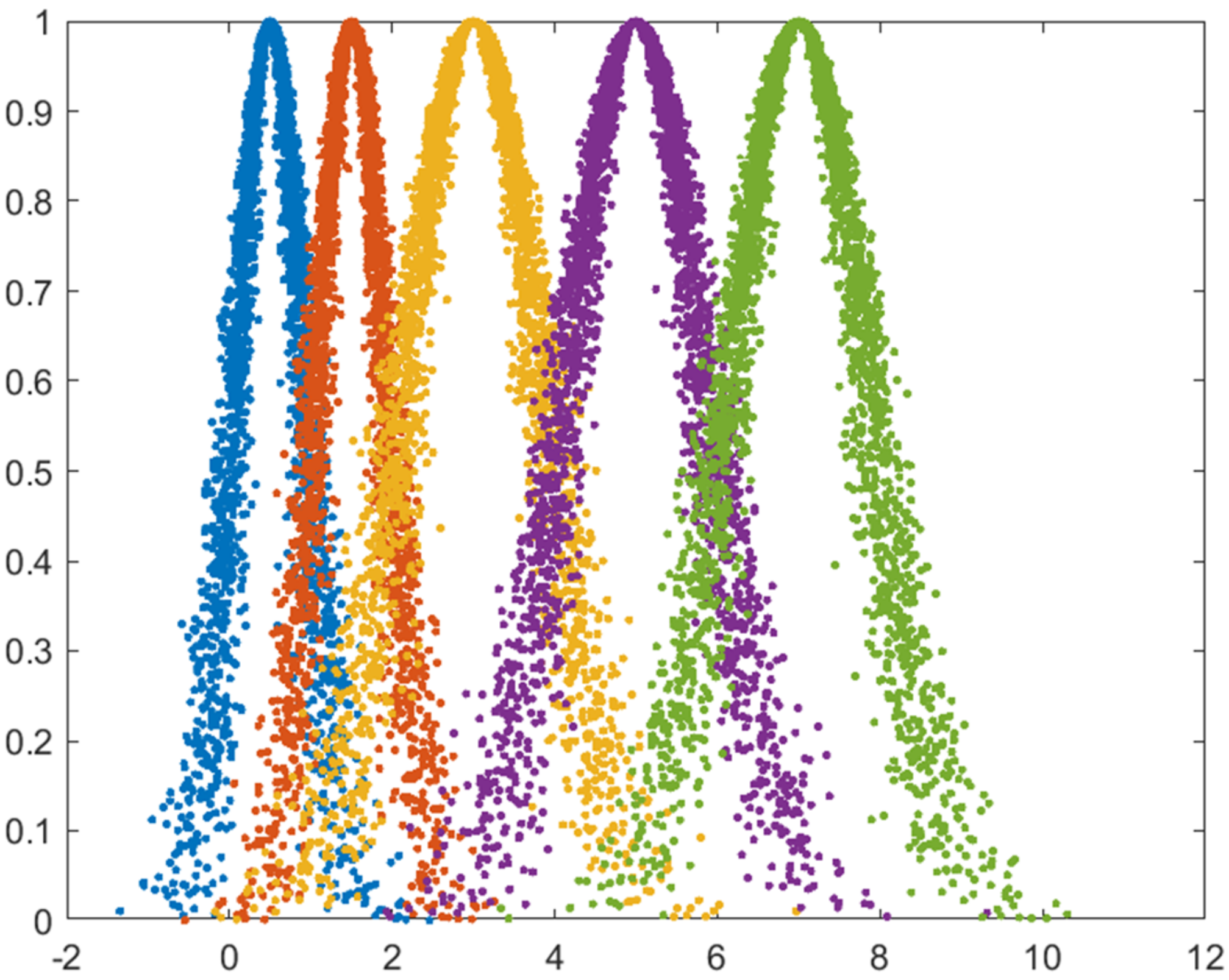
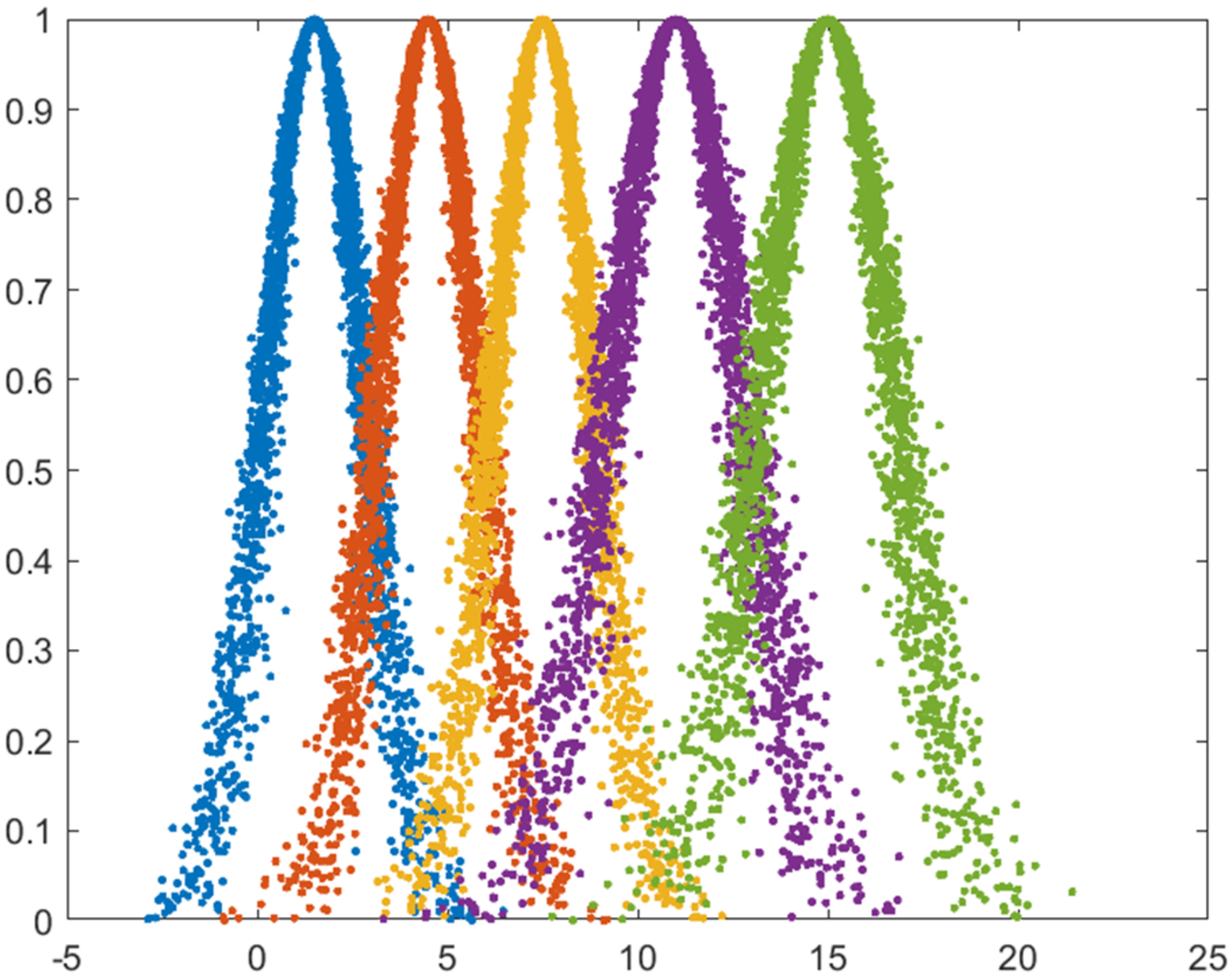
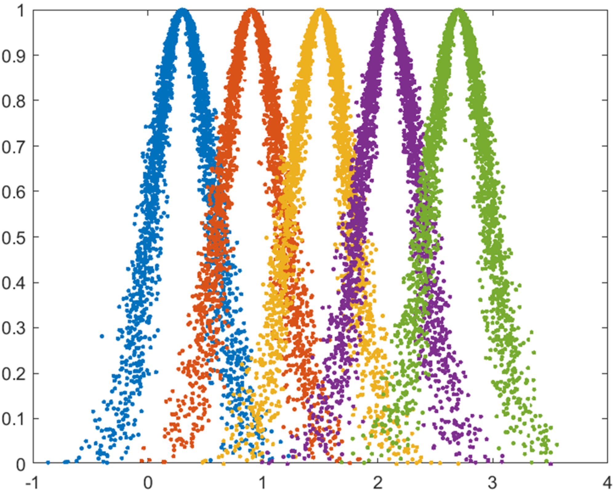
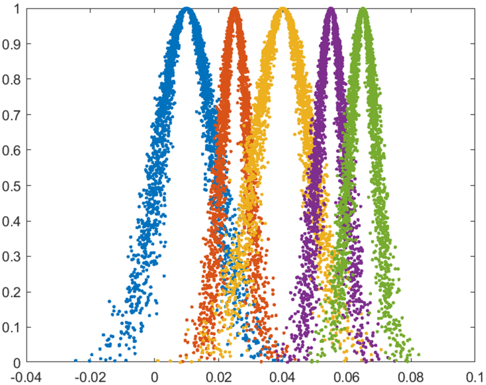
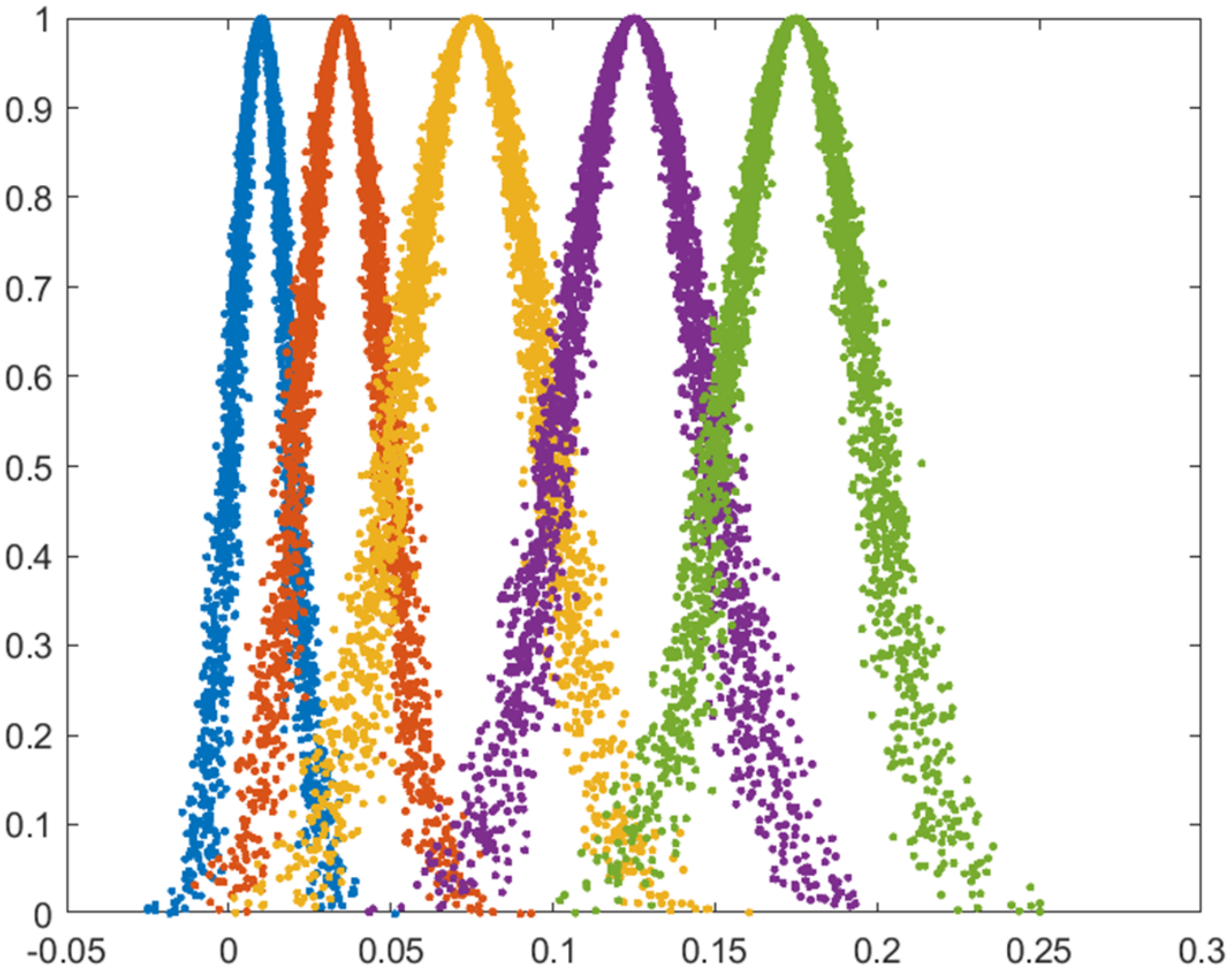
According to the ranking of each indicator in Table 6, the upper and lower critical values $\left[G_{\min },G_{\max }\right]$ were substituted into Equations (6)–(8) to obtain the numerical characteristic values of the cloud model for each indicator, as shown in

Table 7. Numerical feature values of each indicator cloud model.

Grade	Low	Lower	General	Higher	High
X1,1	(1.5, 1.2739, 0.2)	(4.5, 1.2739, 0.2)	(7.5, 1.2739, 0.2)	(11, 1.6985, 0.3)	(15, 1.6985, 0.3)
X1,2	(0.3, 0.2548, 0.05)	(0.9, 0.2548, 0.05)	(1.5, 0.2548, 0.05)	(2.1, 0.2548, 0.05)	(2.7, 0.2548, 0.05)
X1,3	(0.5, 0.4246, 0.1)	(1.5, 0.4246, 0.1)	(3, 0.8493, 0.15)	(5, 0.8493, 0.15)	(7, 0.8493, 0.15)
X1,4	(0.01, 0.0085, 0.0015)	(0.025, 0.0042, 0.001)	(0.04, 0.0085, 0.0015)	(0.055, 0.0042, 0.001)	(0.065, 0.0042, 0.001)
X1,5	(0.01, 0.0085, 0.0015)	(0.035, 0.0127, 0.002)	(0.075, 0.0212, 0.003)	(0.125, 0.0212, 0.003)	(0.175, 0.0212, 0.003)
X2,1	(0.2, 0.1699, 0.03)	(0.6, 0.1699, 0.03)	(1, 0.1699, 0.03)	(1.4, 0.1699, 0.03)	(1.8, 0.1699, 0.03)
X2,2	(0.01, 0.0085, 0.0015)	(0.03, 0.0085, 0.0015)	(0.05, 0.0085, 0.0015)	(0.07, 0.0085, 0.0015)	(0.09, 0.0085, 0.0015)
X2,3	(0.15, 0.1274, 0.02)	(0.45, 0.1274, 0.02)	(0.75, 0.1274, 0.02)	(1.1, 0.1699, 0.03)	(1.5, 0.1699, 0.03)
X2,4	(0.5, 0.4246, 0.1)	(2, 0.8493, 0.15)	(4, 0.8493, 0.15)	(6.5, 1.2739, 0.2)	(9.5, 1.2739, 0.2)
X2,5	(0.06, 0.0510, 0.01)	(0.18, 0.0510, 0.01)	(0.3, 0.0510, 0.01)	(0.42, 0.0510, 0.01)	(0.54, 0.0510, 0.01)
X2,6	(0.01, 0.0085, 0.0015)	(0.03, 0.0085, 0.0015)	(0.05, 0.0085, 0.0015)	(0.07, 0.0085, 0.0015)	(0.09, 0.0085, 0.0015)
X2,7	(0.5, 0.4246, 0.1)	(2, 0.8493, 0.15)	(4, 0.8493, 0.15)	(6, 0.8493, 0.15)	(10, 2.5478, 0.4)
X2,8	(0.01, 0.0085, 0.0015)	(0.03, 0085, 0.0015)	(0.05, 0.0085, 0.0015)	(0.07, 0.0085, 0.0015)	(0.09, 0.0085, 0.0015)
X2,9	(12.5, 10.6157, 1.8)	(37.5, 10.6157, 1.8)	(62.5, 10.6157, 1.8)	(87.5, 10.6157, 1.8)	(105, 4.2463, 0.7)
X2,10	(−2, 0.4246, 0.1)	(−1.25, 0.2123, 0.03)	(−0.8, 0.1699, 0.03)	(−0.45, 0.1274, 0.02)	(−0.15, 0.1274, 0.02)
X3,1	(−0.5, 0.4246, 0.1)	(0.05, 0.0425, 0.01)	(0.2, 0.0850, 0.015)	(0.35, 0.0425, 0.01)	(0.55, 0.0425, 0.01)
X3,2	(−0.5, 0.4246, 0.1)	(0.025, 0.0212, 0.003)	(0.075, 0.0212, 0.003)	(0.125, 0.0212, 0.003)	(0.175, 0.0212, 0.003)
X3,3	(−0.5, 0.4246, 0.1)	(0.025, 0.0212, 0.003)	(0.075, 0.0212, 0.003)	(0.125, 0.0212, 0.003)	(0.175, 0.0212, 0.003)
X3,4	(−0.5, 0.4246, 0.1)	(0.025, 0.0212, 0.003)	(0.075, 0.0212, 0.003)	(0.125, 0.0212, 0.003)	(0.175, 0.0212, 0.003)
X3,5	(−0.5, 0.4246, 0.1)	(0.25, 0.2123, 0.03)	(0.75, 0.2123, 0.03)	(1.5, 0.4246, 0.1)	(2.5, 0.4246, 0.1)
X3,6	(−0.5, 0.4246, 0.1)	(0.025, 0.0212, 0.003)	(0.075, 0.0212, 0.003)	(0.125, 0.0212, 0.003)	(0.175, 0.0212, 0.003)

. The number of cloud drops per cloud was set to 3000, and the cloud model plots for each evaluation metric were derived by plotting the normal cloud model with MATLAB software. The cloud model diagrams for each of the five evaluation indicators included under the level of low carbon logistics environmental support are shown in Figure 4, Figure 5, Figure 6, Figure 7 and Figure 8, for example. The horizontal coordinates represent the range of values of the evaluation factors, the vertical coordinates represent the corresponding affiliation degrees, and the curves from left to right represent the clouds represented by the evaluation levels of “low”, “low”, “average”, “high”, and “high”.

4.2.4. Calculate the Affiliation Degree of Each Index

After getting the cloud model of each evaluation index in the regional logistics low carbonization evaluation index system, we use the X conditional cloud generator of the cloud model by MATLAB programming and take N = 3000 to get the affiliation degree of different levels corresponding to each evaluation index of the province. According to the principle of maximum affiliation degree, select the level corresponding to the maximum of the affiliation degree as the index level, taking Beijing in 2013 as an example, show the results in

Table 8. Indicator affiliation with Beijing 2013 as an example.

Grade	Low	Lower	General	Higher	High	Grade
X1,1	0.0000	0.0006	0.1504	0.8250	0.0222	Higher
X1,2	0.0000	0.0122	0.6359	0.3419	0.0034	General
X1,3	0.0000	0.0000	0.3626	0.6251	0.0095	Higher
X1,4	0.0360	0.1714	0.7032	0.0002	0.0000	General
X1,5	0.0000	0.0001	0.5851	0.4010	0.0027	General
X2,1	0.0000	0.0009	0.1732	0.8858	0.0276	Higher
X2,2	0.0000	0.0000	0.0104	0.6376	0.3473	Higher
X2,3	0.1492	0.9276	0.0324	0.0013	0.0000	Lower
X2,4	0.0000	0.1711	0.8907	0.0850	0.0002	General
X2,5	0.0001	0.0411	0.9385	0.1421	0.0009	General
X2,6	0.0000	0.0000	0.0060	0.4999	0.4717	Higher
X2,7	1.0000	0.2158	0.0013	0.0000	0.0028	low
X2,8	0.0501	0.9780	0.1101	0.0005	0.0000	Higher
X2,9	0.9933	0.0598	0.0002	0.0000	0.0000	low
X2,10	0.0888	0.5643	0.3939	0.0003	0.0000	Higher
X3,1	0.5553	0.0633	0.0191	0.0000	0.0000	low
X3,2	0.4427	0.9992	0.0651	0.0001	0.0000	Higher
X3,3	0.4102	0.3580	0.6335	0.0079	0.0000	General
X3,4	0.3705	0.0239	0.8801	0.1793	0.0006	General
X3,5	0.2948	0.9096	0.0285	0.0179	0.0001	Higher
X3,6	0.3812	0.0439	0.9752	0.1069	0.0003	General
C	0.2233	0.2623	0.3704	0.2311	0.0322	General

.

4.2.5. Entropy Weighting Method to Determine the Weights

Based on the entropy weighting method to calculate the weight of each index in the system, substitute the data of each index into the Equations (1)–(4) by MATLAB programming to calculate the weight of each index, and the results are shown in

Table 9. Standardization of raw data for each indicator in Beijing.

Indicators	2013	2014	2015	2016	2017	2018	2019	Weights
X1,1	0.0000	0.1022	0.2199	0.3793	0.5836	0.8320	1.0000	0.0513
X1,2	0.0000	0.1448	0.4588	0.6264	0.7947	0.9850	1.0000	0.0394
X1,3	0.0000	0.1014	0.2026	0.3108	0.4063	0.8936	1.0000	0.0572
X1,4	0.0000	0.4135	0.5806	0.6921	1.0000	0.5982	0.2522	0.0333
X1,5	0.0094	0.2449	0.0000	0.0078	0.6225	1.0000	0.6693	0.0886
X2,1	0.0000	0.2536	0.3057	0.5095	0.7986	0.8412	1.0000	0.0376
X2,2	0.5565	0.5968	0.5968	0.0000	0.4919	0.4919	1.0000	0.0270
X2,3	0.0000	0.0657	0.1860	0.1370	0.2733	0.6187	1.0000	0.0714
X2,4	0.0000	0.0908	0.1789	0.2689	0.6759	0.6690	1.0000	0.0566
X2,5	0.0000	0.1275	0.1534	0.3029	0.6337	1.0000	0.9851	0.0574
X2,6	1.0000	0.9773	0.7045	0.2841	0.0000	0.2841	0.4091	0.0399
X2,7	0.9301	0.8086	0.2804	0.0000	0.4893	0.7959	1.0000	0.0320
X2,8	1.0000	0.9688	0.4375	0.2188	0.5313	0.6875	0.0000	0.0366
X2,9	0.0000	0.1227	0.1727	0.3893	0.7387	0.9558	1.0000	0.0535
X2,10	0.9048	0.9257	0.9208	0.9327	0.9845	0.0000	1.0000	0.0221
X3,1	0.1527	0.5078	0.1334	0.3445	1.0000	0.4195	0.0000	0.0526
X3,2	0.7394	0.6398	0.3643	0.0000	0.2920	1.0000	0.1378	0.0450
X3,3	0.4169	0.5942	0.1780	0.5118	1.0000	0.9176	0.0000	0.0388
X3,4	0.4426	0.0000	0.0635	0.4529	0.8443	1.0000	0.2275	0.0547
X3,5	1.0000	0.0000	0.0151	0.6839	0.6421	0.0819	0.8127	0.0668
X3,6	0.7899	1.0000	0.3479	0.3325	0.4845	0.0000	0.2899	0.0380

.

4.2.6. Determine the Comprehensive Evaluation Level of Regional Logistics Index

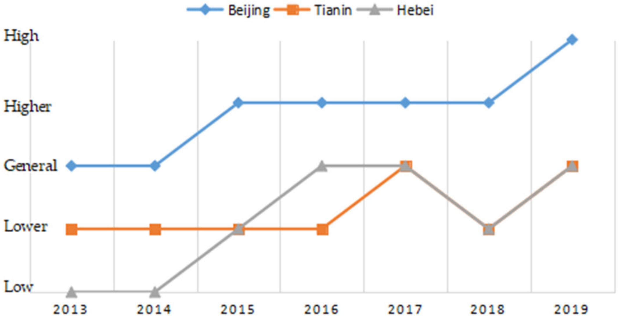
First, the weights and affiliation degrees of each evaluation index are substituted into Equation (11) to obtain the comprehensive determination degree and evaluation grade, for example, the determination degree of each evaluation grade in Beijing in 2013 is $C=\left(0.2204, 0.2689 ,0.3709 ,0.2260 ,0.0315 \right)$. Second, according to the principle of maximum determination degree, select the evaluation grade with the maximum determination degree as the final comprehensive evaluation result, as shown in

Table 10. Evaluation Results of Logistics Decarbonization Development in Beijing from 2013–2019.

Grade	Low	Lower	General	Higher	High	Evaluation Results
2013	0.2204	0.2689	0.3709	0.2260	0.0315	Genera
2014	0.2011	0.2365	0.3887	0.2838	0.0347	Genera
2015	0.2199	0.2262	0.2756	0.3306	0.0398	Higher
2016	0.2052	0.2422	0.2594	0.3657	0.0530	Higher
2017	0.1812	0.1463	0.2054	0.3581	0.1863	Higher
2018	0.2093	0.1874	0.1329	0.3762	0.2357	Higher
2019	0.2202	0.1678	0.1777	0.1642	0.2708	High

,

Table 11. Evaluation Results of Logistics Decarbonization Development in Tianjin 2013–2019.

Grade	Low	Lower	General	Higher	High	Evaluation Results
2013	0.2440	0.3131	0.2515	0.2546	0.0808	Lower
2014	0.2166	0.3202	0.2887	0.2628	0.0486	Lower
2015	0.1852	0.3268	0.2735	0.2599	0.0594	Lower
2016	0.2378	0.3301	0.2310	0.2435	0.0656	Lower
2017	0.1437	0.3075	0.3556	0.2153	0.0661	General
2018	0.1284	0.3849	0.3815	0.1642	0.0623	Lower
2019	0.0741	0.2191	0.3531	0.2450	0.1517	General

and

Table 12. Evaluation Results of Logistics Decarbonization Development in Hebei Province from 2013 to 2019.

Grade	Low	Lower	General	Higher	High	Evaluation Results
2013	0.2859	0.2655	0.2323	0.1925	0.1081	Low
2014	0.3137	0.3102	0.2573	0.1368	0.0664	Low
2015	0.2849	0.3590	0.2781	0.1271	0.0834	Lower
2016	0.2826	0.2778	0.3544	0.1294	0.0526	General
2017	0.2692	0.2677	0.3071	0.1574	0.1307	General
2018	0.1639	0.3536	0.3213	0.1601	0.1493	Lower
2019	0.1619	0.2760	0.3480	0.2277	0.1552	General

. Finally, the Beijing-Tianjin-Hebei regional logistics decarbonization development grade from 2013 to 2019 do the comparison, as shown in Figure 9.

From the time dimension of the comprehensive evaluation results, the overall development of logistics decarbonization in the Beijing-Tianjin-Hebei region from 2013 to 2019 is on an upward trend, with all three regions showing different degrees of improvement. Among them, the development of logistics decarbonization in Beijing develops from average level to high-level, that in Tianjin develops from lower level to average level, and that in Hebei develops from low-level to average level; relatively speaking, the development in Tianjin is slow, which is not in line with its economic level. From the spatial dimension of the comprehensive evaluation results, the development of logistics low-carbon within the Beijing-Tianjin-Hebei region is not balanced, the specific performance is Beijing $\succ$ Tianjin $\succ$ Hebei. There has been a level difference in the development of logistics decarbonization within the Beijing-Tianjin-Hebei region between 2013 and 2019, and the development to 2019, Beijing is at a high-level of development nationwide, while Tianjin and Hebei Province are still at an average level of development, which is two levels away from Beijing in the same region.

4.3. Determination of Influencing Factors and Suggestions for Countermeasures

4.3.1. Determination of Influencing Factors

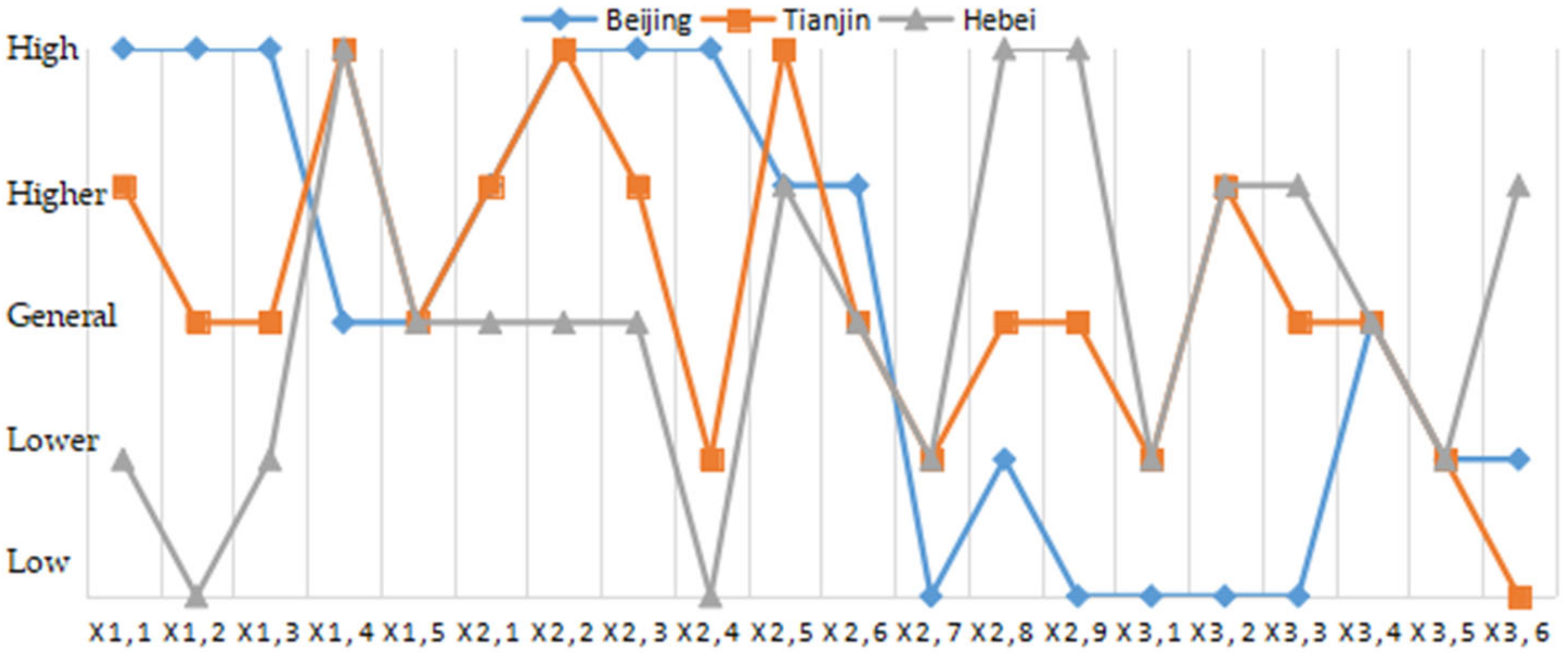
According to the development trend of each index and the horizontal comparison with the three provinces and cities in Beijing, Tianjin and Hebei, the shortcomings of each region in the development of logistics low carbonization are identified, and the main factors affecting the development of logistics low carbonization in the city are found, so as to provide theoretical support for the development of logistics low carbonization. Due to space limitations, the evaluation grade of each indicator is displayed in Beijing region as an example, as shown in

Table 13. Evaluation level of each indicator in Beijing region for example.

Indicators	2013	2014	2015	2016	2017	2018	2019
X1,1	Higher	Higher	Higher	Higher	High	High	High
X1,2	General	Higher	Higher	Higher	High	High	High
X1,3	Higher	Higher	Higher	Higher	Higher	High	High
X1,4	General	General	Higher	Higher	High	Higher	General
X1,5	General	General	General	General	General	General	General
X2,1	Higher	Higher	Higher	Higher	Higher	Higher	Higher
X2,2	Higher	Higher	Higher	Higher	Higher	Higher	High
X2,3	Lower	Lower	General	Lower	General	Higher	High
X2,4	General	General	General	Higher	High	High	High
X2,5	General	General	General	Higher	Higher	Higher	Higher
X2,6	Higher	Higher	Higher	Higher	Higher	Higher	Higher
X2,7	Low	Low	Low	Low	Low	Low	Low
X2,8	Lower	Lower	Lower	Lower	Lower	Lower	Lower
X2,9	Low	Low	Low	Low	Low	Low	Low
X2,10	Lower	General	Lower	General	General	Low	General
X3,1	Low	General	Low	Lower	High	General	Low
X3,2	Lower	Lower	Low	Low	Low	Lower	Low
X3,3	General	General	Lower	General	Higher	Higher	Low
X3,4	General	General	General	General	Higher	Higher	General
X3,5	Lower	Lower	Lower	Lower	Lower	Lower	Lower
X3,6	General	General	Lower	Lower	General	Lower	Lower
C	General	General	Higher	Higher	Higher	Higher	High

; meanwhile, the evaluation grade of each indicator in Beijing, Tianjin and Hebei in 2019 is compared, as shown in Figure 10.

From the evaluation grade of each indicator in Beijing, Tianjin and Hebei provinces and cities, the five indicators of per capita cargo turnover, the contribution rate of logistics industry to GDP, the part of logistics personnel in the workforce, the growth rate of logistics personnel and the growth rate of technical market turnover in Beijing are below the national average level all year, and the development is slow. By 2019, the efficiency of logistics industry, logistics industry input, logistics industry output and technical support are the indicators under the four secondary indicators are still below the national average level, and the shortcomings are more obvious. Tianjin region has been at a low or lower level nationally in the five indicators of per capita e-commerce sales, per capita cargo turnover, growth rate of new fixed asset investment in logistics industry, growth rate of technology market turnover, and growth rate of R&D funding during 2013–2019, and the development has been neglected, a large gap between the levels of the indicators under the low-carbon logistics environment support power and Beijing. Hebei Province has the most obvious gap in low-carbon logistics environment support power relative to neighboring Beijing and Tianjin, mainly in the form of per capita fiscal revenue per year at a low national level, per capita gross regional product and per capita total retail sales of social goods per year at a low-level. In addition, the three indicators of per capita e-commerce sales, per capita turnover of goods and growth rate of technology market turnover in 2019 are still at a low or lower level nationwide.

As can be seen from Figure 10, the development of each indicator in Beijing, Tianjin and Hebei provinces and cities is still in an unbalanced state by 2019, with the biggest difference between Beijing and the other two provinces and cities, as shown because the evaluation levels of each indicator under the two secondary indicators of economic environment and logistics infrastructure are higher than those of Tianjin and Hebei, while the levels of each indicator in logistics industry efficiency and logistics industry input and output are significantly lower than those of the other two provinces and cities; Tianjin is generally higher than Hebei in the four secondary indicators of economic environment, policy environment, logistics infrastructure, and logistics industry scale, but not higher than Hebei in the indicators of low carbon logistics potential. Thus, it seems that although the three provinces and cities in Beijing, Tianjin and Hebei have made breakthroughs in cooperation, they still lack synergy in the development of low-carbon logistics due to the large differences in administrative division, consciousness and economic development level.

4.3.2. Suggestions for Countermeasures to the Low-Carbon Development of Logistics in Beijing-Tianjin-Hebei Region

(1)

From the shortcomings of the development of low-carbon logistics in Beijing, Tianjin and Hebei in recent years, Beijing needs to strengthen two aspects of low-carbon logistics strength and low-carbon logistics potential, especially the three modules of logistics industry efficiency, logistics industry input and demand, and technical support. Tianjin should start with a balanced approach to logistics industry efficiency, input, output, demand and technical support in order to improve the overall low-carbon development of logistics. Hebei Province should strengthen the development of logistics economy, improve the practice base of logistics enterprises, promote industrial clusters and create a logistics ecological chain while improving economic strength, so as to enhance the level of logistics low carbonization in all aspects.

(2)

Strengthen the division of labor and cooperation between Beijing, Tianjin and Hebei in logistics. In the 13th Five-Year Plan, Beijing, Tianjin and Hebei are planned as a whole region, and the respective positions of the three provinces and cities have been clarified. In this context, the logistics industry synergy among the three provinces and cities should optimize the logistics network and divide the work according to the characteristics of each region. Beijing gives full play to the advantages of science and technology and innovates the development of logistics industry while improving the consumer-oriented end logistics system. Tianjin focuses on building a port logistics base in the context of the linkage of three ports. Compare with Beijing and Tianjin, Hebei Province is rich in resources, so it should undertake the transfer of Beijing-Tianjin trade logistics and build Hebei into an important base for modern trade logistics in the country.

(3)

The government increases the policy support for developing low-carbon logistics. The development of low-carbon logistics in Beijing, Tianjin and Hebei needs the cooperation and joint planning of the three regions, and government departments should give support and guidance in policies, such as encouraging the development of ecological logistics industry chain, providing relevant enterprises with corresponding technical support or improving the reasonableness of taxation and financing policy preferences, etc. In addition, while developing regional logistics and economy at high-speed, we should actively promote the idea of green logistics, change the traditional concept of consumers, advocate low-carbon consumption and raise the low-carbon awareness of the logistics industry.

(4)

Improve the level of informatization of low-carbon logistics in Beijing, Tianjin and Hebei. Informatization is an important feature of modern logistics and an effective way to achieve low carbon regional logistics. In the process of integrated development and communication, Beijing, Tianjin and Hebei provinces and cities should break the information silos, establish and improve the logistics information exchange platform, and share and freely exchange logistics information so as to connect the information of each node of the supply chain and give full play to the advantages of regional informatization, to reduce logistics costs and improve logistics efficiency.

5. Conclusions

(1)

Twenty-one indicators are selected from the three dimensions of low-carbon logistics environment support, low-carbon logistics strength and low-carbon logistics potential to establish the regional logistics low-carbonization development evaluation index system. Combined with the cloud model and entropy weight method to build the index evaluation model, which solves the problem of fuzziness and randomness in the process of regional logistics low-carbonization development evaluation.

(2)

The evaluation model of regional logistics decarbonization development can show the development changes of each region in spatial and temporal dimensions and also solve the problem of horizontal comparison between different regions, giving quantitative results of different regions and different times. Then, according to the quantitative results, can discover the shortcomings of regional logistics decarbonization development and provide theoretical support for the further development of regional logistics.

(3)

The entropy weight-cloud model method uses the characteristic indicators that can reflect the complex relationship between multiple factors to derive the corresponding evaluation level. It makes the evaluation results more intuitive and accurate through the cloud diagram and calculation of evaluation level. At the same time, it provides reference for the shortcomings of regional logistics decarbonization development, which is of positive significance to enhance the development of regional logistics decarbonization.

(4)

The development of regional logistics decarbonization is a complex and continuously changing process, and future research can further improve the evaluation index system, optimize the evaluation model, and enhance the accuracy and applicability of the evaluation model.

References

- Butner, K.; Geuder, D.; Hittner, J. Mastering Carbon Management: Balancing Trade-Offs to Optimize Supply Chain Efficiencies; IBM Institute for Business Value: New York, NY, USA, 2008; pp. 2–12. [Google Scholar]
- Dada, A.; Staake, T. Carbon footprints from enterprises to product instances: The potential of the EPC network. In Beherrschbare Systeme-Dank Informatik; Jahrestagung der Gesellschaft für Informatik: München, Germany, 2008; pp. 873–878. [Google Scholar]
- Piecyk, M.I.; Mc Kinnon, A.C. Forecasting the carbon footprint of road freight transport in 2020. Int. J. Prod. Econ. 2010, 128, 31–42. [Google Scholar] [CrossRef]
- Wang, L.P.; Liu, M.H. Research on carbon emission measurement and influencing factors of China’s logistics industry based on input-output method. Resour. Sci. 2018, 40, 195–206. [Google Scholar]
- Liu, Y.; Li, L. Study on decoupling and influencing factors of carbon emissions from logistics industry in China. Environ. Sci. Technol. 2018, 41, 177–181. [Google Scholar]
- Timilsina, G.R.; Shrestha, A. Transport sector CO2 emissions growth in Asia: Underlying factors and policy options. Energy Policy 2009, 37, 4523–4539. [Google Scholar] [CrossRef]
- Yang, L.; Cai, Y.; Zhong, X.; Shi, Y.; Zhang, Z. A Carbon Emission Evaluation for an Integrated Logistics System—A Case Study of the Port of Shenzhen. Sustainability 2017, 9, 462. [Google Scholar] [CrossRef] [Green Version]
- Yang, Y.W.; Wu, A.L.; Zhu, Y.Y. Decomposition and dynamic simulation of carbon emission drivers: Taking Inner Mongolia autonomous region as an example. Stat. Decis. Mak. 2020, 36, 76–80. [Google Scholar]
- Li, F.G.; Wu, L.J. Decomposition of carbon emission drivers based on LMDI method. Stat. Decis. Mak. 2019, 35, 101–104. [Google Scholar]
- Men, D.; Huang, X. Study on influencing factors of carbon emission in Jiangxi Province—Based on LMDI decomposition method. Ecol. Econ. 2019, 35, 31–35. [Google Scholar]
- Wehner, J. Energy Effificiency in Logistics: An Interactive Approach to Capacity Utilisation. Sustainability 2018, 10, 1727. [Google Scholar] [CrossRef] [Green Version]
- Peng, L. Evaluation of low carbon logistics capability of logistics enterprises in China. Bus. Econ. Res. 2017, 10, 87–89. [Google Scholar]
- Xiang, C.; Gong, B.G.; Wu, B.L. Low carbon behavior capability evaluation model of logistics service supply chain. Stat. Decis. Mak. 2017, 5, 67–71. [Google Scholar]
- Jian, L.; Jian, T. Research on the impact of China’s industrial structure adjustment on low carbon logistics efficiency—An empirical analysis based on super efficiency DEA low carbon logistics efficiency evaluation model. Price Theory Pract. 2017, 12, 130–133. [Google Scholar]
- Yang, C.M. Efficiency measurement of Jiangsu logistics industry under low carbon constraints. East China Econ. Manag. 2018, 32, 27–32. [Google Scholar]
- Chaabane, A.; Ramudhin, A.; Paquet, M. Design of sustainable supply chains under the emission trading scheme. Int. J. Prod. Econ. 2012, 135, 37–49. [Google Scholar] [CrossRef]
- Li, C. Research on the development status and countermeasures of low carbon logistics in China. Logist. Eng. Manag. 2018, 40, 1–3. [Google Scholar]
- Dong, Y.X. Research on the development status and trend of China’s low carbon logistics from an international perspective. Price Mon. 2018, 12, 46–49. [Google Scholar]
- Zhang, H. Analysis of low carbon logistics development countermeasures from the perspective of Beijing Tianjin Hebei synergy. Reform Strategy 2016, 32, 118–120. [Google Scholar]
- Zhao, S.L.; Yang, X.Y.; Song, W. General strategy of transportation and logistics integration in Beijing, Tianjin and Hebei from the perspective of low-carbon economy. China Stat. 2017, 12, 6–8. [Google Scholar]
- Ma, Y. Research on Total Factor Productivity of China’s Logistics Industry under Low Carbon Constraints; Northeast University of Finance and Economics: Dalian, China, 2014. [Google Scholar]
- Fei, X. Research on the Coordinated Development of Logistics Industry and Economic Decarbonization; Nanchang University: Nanchang, China, 2015. [Google Scholar]
- Gao, F. Research on the Coordinated Development of China’s Logistics Industry and Low-Carbon Economy; Tianjin University of Technology: Tianjin, China, 2016. [Google Scholar]
- Qin, Y. Analysis of Regional Logistics Efficiency and Its Influencing Factors under Low Carbon Economy; East China Jiaotong University: Nanchang, China, 2015. [Google Scholar]
- Lina, S. Research on the Difference of Low-Carbon Logistics Performance of Regions along the Silk Road Economic Belt in China; Zhengzhou University: Zhenzhou, China, 2018. [Google Scholar]
- Wang, X. Research on the Mechanism and Path of Low-Carbon Development of Regional Logistics; Tianjin University: Tianjin, China, 2017. [Google Scholar]
- Li, D.Y. Uncertain Artificial Intelligence; National Defense Industry Press: Beijing, China, 2005. [Google Scholar]
- Wang, L.; Zhao, H.; Liu, X.; Zhang, Z.L.; Xu-Hui Steve, E. Optimal Remanufacturing Service Resource Allocation for Generalized Growth of Retired Mechanical Products: Maximizing Matching Efficiency. IEEE Access 2021, 9, 89655–89674. [Google Scholar]
- Jia, L.; Yu, Y.; Li, Z.; Qin, S.; Guo, J.; Zhang, Y.; Jin, Y. Study on the Hg0 removal characteristics and synergistic mechanism of iron-based modified biochar doped with multiple metals. Bioresour. Technol. 2021, 332, 125086. [Google Scholar] [CrossRef] [PubMed]
- Xu, Q.W.; Xu, K.L. Evaluation of ambient air quality based on synthetic cloud model. Fresenius Environ. Bull. 2018, 27, 141–146. [Google Scholar]
- Yan, F.; Li, Z.J.; Dong, L.J.; Huang, R.; Cao, R.H.; Ge, J.; Xu, K.L. Cloud model-clustering analysis based evaluation for ventilation system of underground metal mine in alpine region. J. Cent. South Univ. 2021, 28, 796–815. [Google Scholar] [CrossRef]
- Lin, C.J.; Zhang, M.; Li, L.P.; Zhou, Z.Q.; Liu, S.; Liu, C.; Li, T. Risk Assessment of Tunnel Construction Based on Improved Cloud Model. J. Performence Constr. Facil. 2020, 34, 04020028. [Google Scholar] [CrossRef]
- Cong, X.H.; Ma, L. Performance Evaluation of Public-Private Partnership Projects from the Perspective of Efficiency, Economic, Effectiveness, and Equity: A Study of Residential Renovation Projects in China. Sustainability 2018, 10, 1951. [Google Scholar] [CrossRef] [Green Version]
- Li, G.; Zhang, Y.; Wang, H.C. Civil aviation master data recognition method based on cloud model and rough set. Comput. Eng. Des. 2020, 41, 2338–2344. [Google Scholar]
- Sun, Y.B.; Zhang, Y. Research on green development evaluation of coal listed companies based on cloud model. China Min. 2020, 29, 79–85. [Google Scholar]
- Liu, F.; Zhu, X.; Hu, Y.; Ren, L.; Johnson, H. A Cloud Theory-Based Trust Computing Model in Social Networks. Entropy 2017, 19, 11. [Google Scholar] [CrossRef] [Green Version]
- Lai, K. Service capability and performance of logistics service providers. Transp. Res. Part E Logist. Transp. Rev. 2004, 40, 385–399. [Google Scholar] [CrossRef]
- Ma, S.; Meng, Q. Research status and development trend of supply chain logistics capability. Comput. Integr. Manuf. Syst. 2005, 11, 301–307. [Google Scholar]
- Ming, W.; Hao, F. Research on the Development Policy of China’s Logistics Industry; China Planning Press: Beijing, China, 2002; p. 17. [Google Scholar]
- Jiang, J.; Liu, Z. Identification of three important capabilities of logistics enterprises. Logist. Technol. 2005, 7, 18–21. [Google Scholar]
Figure 1.
Positive cloud generator.
Figure 2.
Inverse cloud generator.
Figure 3.
Conditional cloud generator.
Figure 4.
Per capita gross regional product cloud model.
Figure 5.
Per capita fiscal revenue cloud model.
Figure 6.
Retail sales of social goods per capita.
Figure 7.
Cloud model of total expenditure ratio of per capita financial environmental protection expenditure.
Figure 8.
Logistics industry as a percentage of fixed asset investment cloud model.
Figure 9.
2013–2019 Beijing-Tianjin-Hebei Regional Logistics Decarbonization Development Grade Comparison.
Figure 10.
2019 Beijing-Tianjin-Hebei comparison of evaluation ratings for each indicator.